Interpreting Mass via Riemannian PolyhedraThanks: P. Miao’s research was partially supported by NSF grant DMS-1906423.

The scalar curvature of a Riemannian manifold is a basic curvature quantity of the metric. Besides prolific motivations from Riemannian geometry, an important incentive to study the scalar curvature is from Einstein’s theory of general relativity. We briefly outline this relativistic role of scalar curvature below.

Suppose $\mathcal{S}^{4}$ is a spacetime, i.e. a time-oriented Lorentz $4$-manifold. Suppose $M^{3}$ is a spacelike hypersurface with a unit normal $n$ in $\mathcal{S}$. By the Einstein equation and the Gauss equation,

(1.1)

$$R(g)-|K|_{g}^{2}+(\mbox{tr}_{g}K)^{2}=16\pi\,T(n,n).$$

Here $R(g)$ is the scalar curvature of the Riemannian metric $g$ on $M$, $K$ is the second fundamental form of $M$ in $\mathcal{S}$, and $T$ is the stress energy tensor determined by matter distribution in $\mathcal{S}$.

A physically reasonable spacetime often satisfies suitable energy conditions which guarantee $T(n,n)\geq 0$. In this case, if $M$ is a maximal slice, i.e. $\mbox{tr}_{g}K=0$, then (1.1) implies $R(g)\geq 0$. In general, under an assumption that $\mathcal{S}$ satisfies the dominant energy condition, study of the triple $(M,g,K)$ often can be related to the case of $R(g)\geq 0$ (see [32] for instance).

If the spacetime $\mathcal{S}$ models an isolated system, the Riemannian manifold $(M,g)$ is often assumed to be asymptotically flat. For such manifolds, a fundamental result on nonnegative scalar curvature metrics is the Riemannian positive mass theorem.

We recall the definitions of asymptotically flat manifolds and their mass.

For an asymptotically flat $(M^{n},g)$, its mass (introduced by Arnowitt, Deser and Misner [4]), is defined as

(1.3)

$$\mathfrak{m}(g)=\lim_{r\rightarrow\infty}\frac{1}{2(n-1)\omega_{n-1}}\int_{S_{r}}(g_{ij,i}-g_{ii,j})\,\bar{\nu}^{j}\,d\bar{\sigma}.$$

Here $S_{r}$ is the coordinate sphere $\{|x|=r\}$, $d\bar{\sigma}$ denotes the Euclidean volume element on $S_{r}$, $\bar{\nu}$ is the Euclidean outward unit normal to $S_{r}$, and summation is applied over repeated indices. It was proved by Bartnik [5], and also by Chruściel [10], that $\mathfrak{m}(g)$ is independent on the choice of coordinates satisfying (1.2).

For dimensions $n\leq 7$, Schoen had a proof of the positive mass theorem in [30]. For arbitrary dimensions, the theorem was shown by Schoen-Yau [33]. A different approach was provided by Lohkamp [22, 23, 24, 25].

In Riemannian geometry, comparison theorems are useful tools in understanding manifolds with various notions of lower curvature bounds. In two dimensions, scalar curvature reduces to Gauss curvature, and geometric triangles were compared to those in a model space (see [1, 2, 35] for instance).

In [14], Gromov suggested Riemannian polyhedra play a useful role in the study of scalar curvature in higher dimensions. Given a convex polyhedron $P$ in $(\mathbb{R}^{n},\bar{g})$, the Euclidean space, Gromov [14, 15] conjectured that, if $g$ is a Riemannian metric on $P$ satisfying

• •

  $g$ has nonnegative scalar curvature;

• •

  each face of $P$ has nonnegative mean curvature in $(P,g)$; and

• •

  along each edge of $P$, the dihedral angle of $(P,g)$ is less than or equal to the corresponding dihedral angle of $P$ in $(\mathbb{R}^{n},\bar{g})$,

then $(P,g)$ is isometric to a polyhedron in $(\mathbb{R}^{n},\bar{g})$.

Significant progress toward this conjecture was obtained by Li [18, 19, 20]. In $3$-dimension, Li [18] proved the conjecture for a wide class of polyhedra including cubes and $3$-simplices. In higher dimensions, Li [19] showed the conjecture holds for a class of prisms with dimensions less than or equal to $7$. In [20], Li extended the comparison theory to metrics with a negative scalar curvature lower bound.

An immediate connection between Gromov’s conjecture and the positive mass theorem is that the conjecture being valid for a single polyhedron implies the latter. This is because, by the work of Lohkmap [21], if the mass of an asymptotically flat $(M,g)$ is negative, the metric $g$ can be deformed to another metric $\tilde{g}$ with nonnegative scalar curvature, which is exactly Euclidean outside a compact set. In this case, by considering a large polyhedron enclosing the nontrivial geometry in the compact set, one would obtain a contradiction to Gromov’s conjecture (see [19, Theorem 5.2] for details).

For an asymptotically flat $3$-manifold $(M,g)$, a connection between the mass $\mathfrak{m}(g)$ and large Riemannian cubes was found in [26].

If $(M^{3},g)$ is complete with nonnegative scalar curvature, the positive mass theorem (Theorem 1.1) shows $\mathfrak{m}(g)>0$, unless $(M,g)$ is isometric to $\mathbb{R}^{3}$. This combined with (3.1) shows

(3.2)

$$-\frac{1}{8\pi}\int_{\mathcal{F}}H\,d\sigma+\frac{1}{8\pi}\int_{\mathcal{E}}\left(\alpha-\frac{\pi}{2}\right)\,ds\geq 0,\ \text{for large}\ L.$$

A related but yet different formula, relating $\mathfrak{m}(g)$ to $C^{3}_{L}$, was also derived in [26].

The quantity $\mathfrak{m}^{(2)}_{k}(t,L)$ measures the angle deficit of the (large) portion of the coordinate plane $\{x^{k}=t\}$ inside the cube $C^{3}_{L}$. (3.3) shows the mass of $(M^{3},g)$ can be obtained by suitably integrating such angle deficit associated to all coordinate planes. It is worthy of noting that, in the setting of asymptotically conical surfaces, the angle deficit can be used to define the $2$-dimensional “mass” of those surfaces (see [9, 7] for instance).

Formula (3.3) was largely prompted by a recent monumental work of Stern [34] that relates the scalar curvature and the level sets of harmonic functions (and maps). Together with the Gauss-Bonnet theorem and Stern’s formula from [34], (3.3) provides insight into the recent new proof of the $3$-dimensional positive mass theorem by Bray-Kazaras-Khuri-Stern [6]. Below we briefly outline this implication following [26, Remark 5].

Stern’s formula [34, equation (14)], in its simplest form, shows

(3.5)

$$\Delta|\nabla u|=\frac{1}{2|\nabla u|}\left[|\nabla^{2}u|^{2}+|\nabla u|^{2}(R-2K_{{}_{\Sigma}})\right],$$

near points where $\nabla u\neq 0$. Here $u$ is a harmonic function on a $3$-manifold $(M^{3},g)$, $R$ and $K_{{}_{\Sigma}}$ denote the scalar curvature of $g$ and the Gauss curvature of $\Sigma$, the level set of $u$, respectively.

Suppose the manifold $(M^{3},g)$ is asymptotically flat. An observation of Bartnik [5] was

(3.6)

$$\sum_{i=1}^{3}\int_{S_{\infty}}\frac{1}{2}\frac{\partial}{\partial\nu}|\nabla y_{i}|^{2}\,d\sigma=16\pi\mathfrak{m}(g).$$

Here $\{y_{i}\}$ are harmonic coordinates on $(M,g)$ near infinity, and $\int_{S_{\infty}}$ represents the limit of integration along a sequence of suitable surfaces approaching infinity. Since $|\nabla y_{i}|$ tends to $1$ suitably fast, it is easily checked that (3.6) is equivalent to

(3.7)

$$\sum_{i=1}^{3}\int_{S_{\infty}}\frac{\partial}{\partial\nu}|\nabla y_{i}|\,d\sigma=16\pi\mathfrak{m}(g).$$

Considering (3.5) and (3.7), one may want to seek a formula that computes $\mathfrak{m}(g)$ in terms of the level sets of $y_{i}$. This was the motivation to the derivation of (3.3) in [26]. It turned out that (3.3) itself does not require $\{x_{i}\}$ to be harmonic.

Next, for simplicity, suppose $M$ has no boundary. Consider a harmonic map

(3.8)

$$U=(u_{1},u_{2},u_{3}):(M,g)\rightarrow(\mathbb{R}^{3},\bar{g})$$

such that $U$ is a diffeomorphism near infinity, and, in this coordinate chart defined by $U$, $g$ satisfies (1.2). By the usual construction of harmonic coordinates (for instance Theorem 3.1 in [5]), such a map $U$ always exists. If one further supposes the regular level set $\Sigma_{t}^{(i)}$ of each $u_{i}$ satisfies $\chi(\Sigma_{t}^{(i)})\leq 1$ (which is the case if $M$ is $\mathbb{R}^{3}$ for instance), then it follows from Stern’s formula (3.5), Bartnik’s formula (3.7), the mass formula (3.3), and the Gauss-Bonnet theorem that

(3.9)

$$\begin{split}&\ 24\pi\,\mathfrak{m}(g)\\ =&\ \lim_{L\to\infty}\sum_{k=1}^{3}\int_{\partial C^{3}_{L}}\frac{\partial}{\partial\nu}|\nabla u_{k}|\,d\sigma+\lim_{L\to\infty}\sum_{k=1}^{3}\int_{-L}^{L}\left[(2\pi-\beta^{\langle k\rangle}_{t})-\int_{C^{(k)}_{t}}\kappa^{(k)}\,ds\right]\,dt\\ \geq&\ \sum_{i=1}^{3}\ \int_{M}\frac{1}{2}\left[\frac{1}{|\nabla u_{i}|}|\nabla^{2}u_{i}|^{2}+R|\nabla u_{i}|\right]dV.\end{split}$$

In particular, if $R\geq 0$, then $\mathfrak{m}(g)\geq 0$. We remark that inequality (3.9) is weaker than the result in [6]. The lower bound of $\mathfrak{m}(g)$ in Theorem 1.2 of [6] only used a single harmonic function.

A potentially useful feature of the above mapping setting (3.9) is the following. Suppose $g_{ij}=g(\partial_{u_{i}},\partial_{u_{j}})$. Given any constant $\Lambda>0$, let $r_{o}>0$ be a constant such that

$$|g_{ij}|\leq\Lambda\ \ \mathrm{and}\ \ |g^{ij}|\leq\Lambda,\ \ \mathrm{if}\ |u|\geq r_{o}.$$

Using the fact $|\nabla u_{i}|^{2}=g^{ii}$ and $\nabla^{2}u_{i}(\partial_{u_{k}},\partial_{u_{l}})=-\Gamma^{i}_{kl}$, we see from (3.9) that, if the scalar curvature is nonnegative, then

(3.10)

$$\mathfrak{m}(g)\geq C\int_{|u|\geq r_{o}}\sum_{i,j,k}|\partial_{i}g_{jk}|^{2},$$

where $C$ is a constant depending only on $\Lambda$. This shows, outside a large $u$-coordinate sphere $\{|u|=r_{o}\}$, the $L^{2}$-norm of $\partial g$ is controlled by the mass.

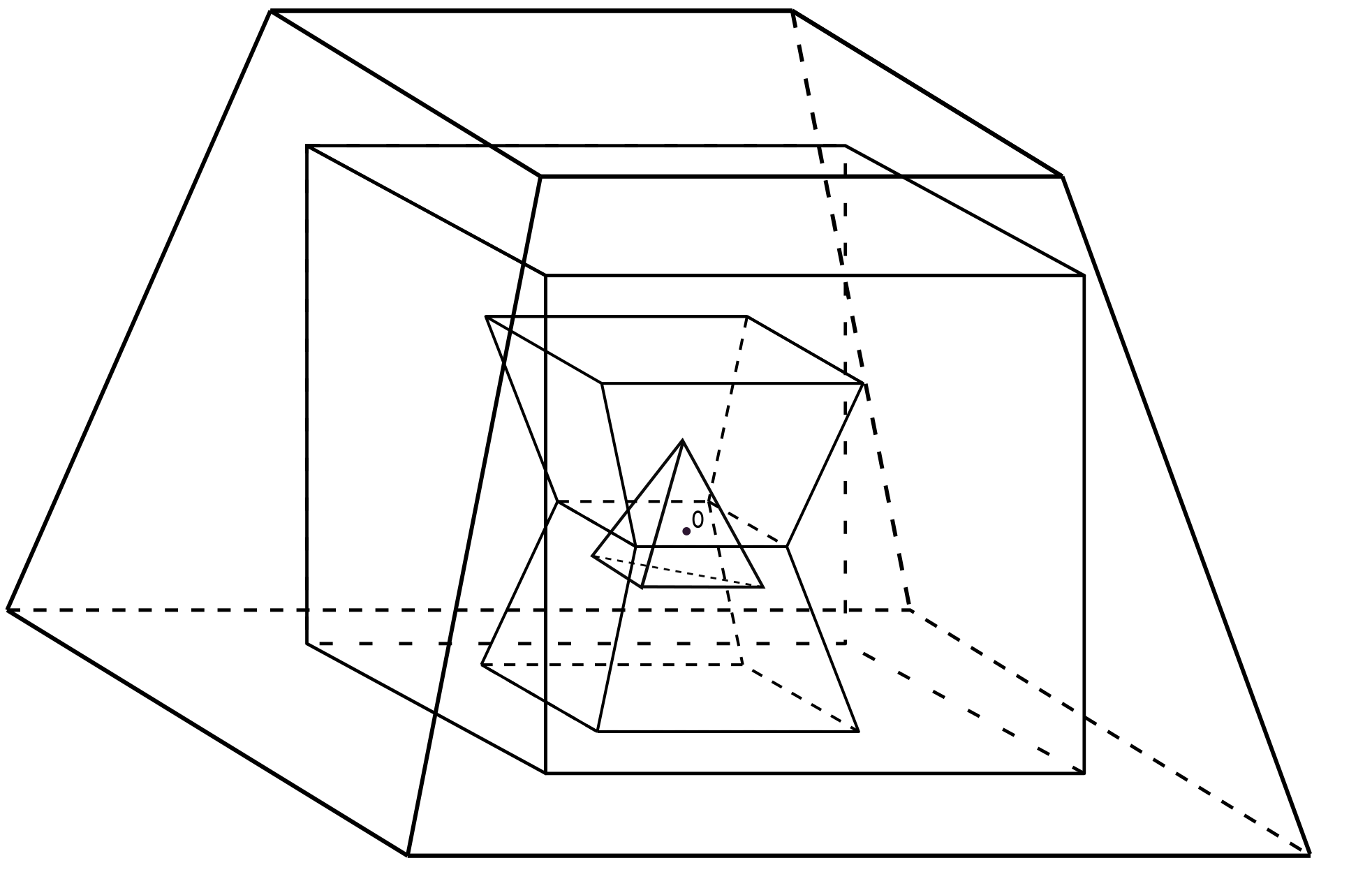
Motivated by Theorem 3.1, Piubello and the author [27] considered a sequence of polyhedra of general types, approaching infinity in an asymptotically flat manifold of arbitrary dimensions.

The sequence $\{P_{k}\}$ in Theorem 4.1 has the feature that it can consist of different types of polyhedra. Moreover, elements in $\{P_{k}\}$ can be non-convex. The angle condition

$$|\sin\bar{\alpha}|\geq c$$

is imposed due to $y^{\prime}(x)=-\frac{1}{\sin y}$ if $y=\arccos x$. In the proof of Theorem 4.1 in [27], one obtains the dihedral angle from the metric coefficients. A condition of $|\sin\bar{\alpha}|\geq c$ helps to convert estimates on the metric to estimates on the dihedral angle.

We briefly comment on the proof of Theorem 4.1. Formula (4.1) was essentially revealed by a special structure that is present in the linearization of the mean curvature function.

To explain this structure, we fix some notations. Let $\Sigma^{n-1}\subset M^{n}$ be a given hypersurface. Let $g$, $\bar{g}$ be two Riemannian metrics on $M$, and let $\gamma$, $\bar{\gamma}$ denote the metrics on $\Sigma$ induced from $g$, $\bar{g}$, respectively. Let $\nu$ and $\bar{\nu}$ be the corresponding unit normal vectors to $\Sigma$ in $(M,g)$ and $(M,\bar{g})$. We assume $\nu$ and $\bar{\nu}$ point to the same side of $\Sigma$. Let $A$, $H$ and $\bar{A}$, $\bar{H}$ denote the second fundamental form, the mean curvature function of $\Sigma$ in $(M,g)$ and $(M,\bar{g})$, respectively. Viewing $\bar{g}$ as a background metric, we write $g=\bar{g}+h$ and assume $|h|_{\bar{g}}<\epsilon(n)$, where $\epsilon(n)$ is a small positive constant depending only on $n$. Here $|\cdot|_{\bar{g}}$ denotes the norm with respect to $\bar{g}$.

We see that, on the right side of (4.2), the first term $(d\,\mbox{tr}_{\bar{g}}\,h-\mbox{div}_{\bar{g}}\,h)(\bar{\nu})$ relates to the mass integral; the divergence term $\mbox{div}_{\bar{\gamma}}X$, upon integration by parts, produces the angle along the edges; and the third term, involving the second fundamental form $\bar{A}$, indicates the advantage of making use of a polyhedron, whose faces are totally geodesic.

Similar to (3.2), if $(M^{n},g)$ is complete, asymptotically flat and has nonnegative scalar curvature, it follows from the positive mass theorem and (4.1) that

(4.3)

$$-\int_{\mathcal{F}(\partial P_{k})}H\,d\sigma+\int_{\mathcal{E}(\partial P_{k})}(\alpha-\bar{\alpha})\,d\mu\geq 0,\ \text{for large }k.$$

Here $\{P_{k}\}$ is any sequence of Euclidean polyhedra satisfying conditions in Theorem 4.1. In particular, for a fixed Euclidean polyhedron $P$,

(4.4)

$$-\int_{\mathcal{F}_{(r)}}H\,d\sigma+\int_{\mathcal{E}_{(r)}}(\alpha-\bar{\alpha})\,d\mu\geq 0,\ \text{for large }r,$$

where $\mathcal{F}_{(r)}$ and $\mathcal{E}_{(r)}$ are the faces and edges of the polyhedron $P_{(r)}$ that is obtained by scaling $P$ by a constant $r$.

As illustrated by Theorem 3.2, it is worthy of taking $\{P_{k}\}$ as a sequence of large coordinate cubes in $(M^{n},g)$. Cubes have a feature that, when sliced by hyperplanes parallel to their face, the resulting intersections are large $(n-1)$-dimensional cubes.

The following can be viewed as a higher dimensional analog of Theorem 3.2.

We explain the quantity $\mathfrak{m}_{k}^{(n-1)}(t,L)$. Let $C^{n}_{L}$ denote a coordinate cube in $(M,g)$, with its center at the coordinate origin and side (coordinate) length $2L$. For every $t\in[-L,L]$ and $k\in\{1,\cdots,n\}$, let $S_{t}^{(k)}$ be the intersection of $\partial C^{n}_{L}$ with the coordinate hyperplane $\{x_{k}=t\}$, i.e.

$$S_{t}^{(k)}=\partial C^{n}_{L}\cap\{x_{k}=t\}.$$

Then $S_{t}^{(k)}$ is the boundary of an $(n-1)$-dimensional cube in $\{x_{k}=t\}$ (see Figure 3). On the hypersurface $\{x_{k}=t\}$, let $\tilde{H}^{(k)}$ be the mean curvature of each face of $S_{t}^{(k)}$ with respect to the outward normal $\tilde{\nu}^{(k)}_{i}$ and let $\tilde{\alpha}^{(k)}$ be the dihedral angle along every edge of $S^{(k)}_{t}$, both taken with respect to $g$.

Associated to each $S^{(k)}_{t}$ in $\{x_{k}=t\}$, $m_{k}^{(n-1)}(t,L)$ is given by

(4.7)

$$\begin{split}&\ \mathfrak{m}_{k}^{(n-1)}(t,L)\\ =&\ \frac{1}{(n-2)\omega_{n-2}}\left(-\int_{\mathcal{F}(S^{(k)}_{t})}\tilde{H}^{(k)}d\sigma^{n-2}+\int_{\mathcal{E}(S_{t}^{(k)})}\left(\tilde{\alpha}^{(k)}-\frac{\pi}{2}\right)d\mu^{n-3}\right),\end{split}$$

where $d\sigma^{n-2}$ and $d\mu^{n-3}$ denote the volume forms, induced from the metric $g$, on the faces and edge of $S^{(k)}_{t}$. The assertion

$$\mathfrak{m}(g|_{\{x_{k}=t\}})=\lim_{L\to\infty}\mathfrak{m}_{k}^{(n-1)}(t,L)$$

is a direct consequence of Theorem 4.1, where $g|_{\{x_{k}=t\}}$ denotes the metric on $\{x_{k}=t\}$ induced from $g$. In many cases, for instance if $g$ has a decay rate of $p>n-3$, this limit will be zero as $\mathfrak{m}(g|_{\{x_{k}=t\}})=0$.

A couple of questions arise in relation to Theorems 4.1 and 4.2.

• a)

  The angle condition $|\sin\bar{\alpha}|\geq c$ serves only as a sufficient condition for (4.1). It would be good to weaken this condition. For instance, a replacement of $|\sin\bar{\alpha}|\geq c$ by a suitable slow decay condition of $\sin\bar{\alpha}$, relative to the growth of the volume of the faces and edges, may be desirable.

• b)

  In dimension three, formula (3.3) combined with the Gauss-Bonnet theorem and Stern’s work [17] yielded a proof of the positive mass theorem. Could formula (4.6) play a role in any new proof of the positive mass theorem in high dimensions?

The preceding connection between polyhedra and the mass of asymptotically flat manifolds prompts one to consider if an analogous connection exists on manifolds that are asymptotically hyperbolic.

We recall the definition of asymptotically hyperbolic manifolds and their mass functional following the work of Chruściel and Herzlich [13]. Let $(\mathbb{H}^{n},\bar{g})$ denote the standard hyperbolic space with constant sectional curvature $-1$. One model of $\mathbb{H}^{n}$ is the upper hyperboloid in the Minkowski spacetime

$$\mathbb{H}^{n}=\{(z,t)\in\mathbb{R}^{n,1}\ |\ z_{1}^{2}+\cdots+z_{n}^{2}-t^{2}=-1,t>0\}.$$

Let $r=|z|$. A Riemannian manifold $(M^{n},g)$ is called asymptotically hyperbolic if there exist a compact set $K\subset M$ and a diffeomorphism $\Phi:M\setminus K\to\mathbb{H}^{n}\setminus D$, where $D$ is some compact set in $\mathbb{H}^{n}$, such that $h:=(\Phi^{-1})^{*}g-\bar{g}$ satisfies

$$|h|_{\bar{g}}+|\bar{D}h|_{\bar{g}}+|{\bar{D}}^{2}h|_{\bar{g}}=O(r^{-q}),\ \text{for some rate}\ q>\frac{n}{2},$$

as $r\to\infty$, and

$$\int_{M}r\left[R_{g}+n(n-1)\right]\,dV_{g}<\infty.$$

Here $R_{g}$ and $dV_{g}$ are the scalar curvature and the volume element of $g$, respectively. The mass functional of $(M,g)$ is a linear functional

(5.1)

$$\mathfrak{m}(\cdot):\mathcal{S}(\mathbb{H}^{n})\longrightarrow\mathbb{R},$$

where $\mathcal{S}(\mathbb{H}^{n})$ is the space of static potentials on $\mathbb{H}^{n}$, given by

(5.2)

$$\mathcal{S}(\mathbb{H}^{n})=\text{span}\{t,z_{1},\cdots,z_{n}\},\ \text{where}\ t=\sqrt{1+r^{2}},$$

and, $\forall\,V\in\mathcal{S}(\mathbb{H}^{n})$,

(5.3)

$$\mathfrak{m}(V)=\lim_{r\to\infty}\int_{|z|=r}\left[V\,(\mbox{div}_{\bar{g}}h-d\mathrm{tr}_{\bar{g}}h)+(\mathrm{tr}_{\bar{g}}h)dV-h({\bar{\nabla}}V,\cdot)\right](\bar{\nu})\,d\bar{\sigma}.$$

Here $d\bar{\sigma}$ is the volume element on the coordinate sphere $\{|z|=r\}$ in $\mathbb{H}^{n}$ and $\bar{\nabla}$ denotes the gradient on $(\mathbb{H}^{n},\bar{g})$. Similar to the asymptotically flat case, the limit of the above integral can be computed along other suitable exhaustion sequences of $M$ (see [28] for instance).

It is common to represent $\mathfrak{m}(\cdot)$ by an $(n+1)$-vector $(p_{0},p_{1},\ldots,p_{n})$ with

$$p_{0}=\mathfrak{m}(t),\ \ p_{i}=\mathfrak{m}(z_{i}),\ \forall\,i=1,\ldots,n.$$

The Riemannian positive mass theorem for asymptotically hyperbolic manifolds states that, if $R_{g}\geq-n(n-1)$, then $p_{0}^{2}\geq\sum_{i=1}^{n}p_{i}^{2}$, and equality holds if and only if $(M,g)$ is isometric to $\mathbb{H}^{n}$. The proof of this theorem has a rich history. We refer readers to [36, 38, 13, 3, 11, 12, 16, 29] and references therein.

Given a function $V$, let $\mathbb{U}(V)(\cdot)$ be the associated $1$-form

(5.4)

$$\mathbb{U}(V)(\cdot)=V\,(\mbox{div}_{\bar{g}}h-d\mbox{tr}_{\bar{g}}h)+(\mbox{tr}_{\bar{g}}h)dV-h({\bar{\nabla}}V,\cdot).$$

The following formula, which can be viewed as a weighted version of Proposition 4.1, was derived by Jang and the author in [17].

Formula (5.5) suggests that when evaluating the total flux of $\mathbb{U}(V)(\cdot)$ across a hypersurface $\Sigma$ with normal $\bar{\nu}$, one likes to simplify the term

(5.6)

$$\mathbb{A}(V,\Sigma):=(\mathrm{tr}_{\bar{\gamma}}h)dV(\bar{\nu})-V\langle\bar{A},h\rangle_{\bar{\gamma}}.$$

In the asymptotically flat case, $V=1$ and one can take $\Sigma$ as hyperplanes which have $\bar{A}=0$. In the asymptotically hyperbolic case, it is natural to first consider those $\Sigma\subset\mathbb{H}^{n}$ which are totally umbilic, i.e.

(5.7)

$$\bar{A}=\frac{1}{n-1}\bar{H}\bar{\gamma}.$$

Under this assumption,

(5.8)

$$\begin{split}\mathbb{A}(V,\Sigma)=&\ \left(\frac{\partial V}{\partial\bar{\nu}}-\frac{\bar{H}}{n-1}V\right)\mathrm{tr}_{\bar{\gamma}}h\\ =&\ \left(\frac{\partial}{\partial\bar{\nu}}\ln V-\frac{\bar{H}}{n-1}\right)V\,\mathrm{tr}_{\bar{\gamma}}h,\ \text{if}\ V\neq 0.\end{split}$$

Some basic choices of pairs $(V,\Sigma)$ making $\mathbb{A}(V,\Sigma)=0$ can be described as follows. Consider the upper half space model of $\mathbb{H}^{n}$,

$$\mathbb{H}^{n}=\{(y_{1},y_{2},\ldots,y_{n})\ |\ y_{1}>0\},\ \bar{g}=\frac{1}{y_{1}^{2}}(dy_{1}^{2}+\cdots+dy_{n}^{2}).$$

One knows

$$y_{1}^{-1}=t-z_{1}\in\mathcal{S}(\mathbb{H}^{n}).$$

Take $V=y_{1}^{-1}$, and choose $\Sigma$ to be

• (i)

  a horosphere given by $\Sigma=\{y_{1}=c\}$ for some constant $c>0$;

• (ii)

  a totally geodesic piece that is isometric to $\mathbb{H}^{n-1}$, say $\Sigma=\{y_{\alpha}=d\}$ for some constant $d$, where $\alpha\in\{2,\ldots,n\}$.

It is easily seen $\mathbb{A(}V,\Sigma)=0$ on such an $\Sigma$.

Making use of these facts, Jang and the author derived the following in [17].

The content of Theorem 5.1 was contained in [17, Remark 3.2]. Though its part (a) could be thought as an analogue of Theorem 3.1 or 4.1, its part (b) shows that, in contrast to the asymptotically flat case (see Remark 4.2), the limit of the integral of the angle deficit along the edges of $P_{L}$, and the integral of the mean curvature difference on most part of the faces of $P_{L}$, do not contribute to $p_{0}-p_{1}$, if $q\geq n-1$. Exploring this fact, Jang and the author [17] derived an evaluation formula of $p_{0}-p_{1}$ using horospheres $\{y_{1}=e^{-L}\}$ alone.

It is worth of seeking other candidates $\Sigma$ on which $\mathbb{A}(V,\Sigma)$ can be simplified with $V=y_{1}^{-1}$. In [8], Chai found that $\mathbb{A}(V,\Sigma)=0$ if $\Sigma$ is any $y$-coordinate hyperplane. This can be seen as follows. Given an arbitrary

$$\Sigma^{n-1}\subset\mathbb{H}^{n}=\{(y_{1},y_{2},\ldots,y_{n})\ |\ y_{1}>0\},$$

if $A_{{}_{E}}$, $H_{{}_{E}}$ denote its second fundamental form, mean curvature with respect to the background Euclidean metric $dy^{2}$, standard conformal transformation formulae give

(5.9)

$$\bar{A}=VA_{{}_{E}}+\frac{\partial V}{\partial\nu_{{}_{E}}}\gamma_{{}_{E}},$$

where $\nu_{{}_{E}}$ is the Euclidean unit normal and $\gamma_{{}_{E}}$ is the background metric on $\Sigma$. Clearly, (5.7) holds if and only if

(5.10)

$$A_{{}_{E}}=\frac{H_{{}_{E}}}{n-1}\gamma_{{}_{E}}.$$

Under this assumption,

(5.11)

$$V^{-1}dV(\bar{\nu})-\frac{\bar{H}}{n-1}=-\frac{H_{{}_{E}}}{n-1}V^{-1}.$$

Therefore, (5.8) becomes

(5.12)

$$\mathbb{A}(V,\Sigma)=\left\{\begin{array}[]{ll}0,&\text{if}\ H_{{}_{E}}=0\\ -\frac{H_{{}_{E}}}{n-1}\,\mbox{tr}_{\bar{\gamma}}h,&\text{if}\ H_{{}_{E}}\neq 0.\end{array}\right.$$

Here $H_{{}_{E}}$ is necessarily a constant. Taking $H_{{}_{E}}=0$, one sees $\mathbb{A}(V,\Sigma)=0$ along any coordinate hyperplanes $\Sigma$ in $\{(y_{1},y_{2},\ldots,y_{n})\}$. Thus, as pointed out by Chai in [8], an analogous statement to part (a) of Theorem 5.1 holds for an exhaustion sequence consisting of $y$-coordinate polyhedra.

References

- [1] A. D. Alexandrov, 1948. Instrinsic geometry of convex surfaces (Russian edition). OGIZ, Moscow-Leningrad. (German edition). Akademie-Verlag, Berlin, 1955. (English edition). In: Kutateladze,S.S. (Ed.), A.D. Alexandrov Selected Works. Part II. Chapman & Hall/CRC, Boca Raton, 2006.
- [2] A. D. Aleksandrov, A theorem on triangles in a metric space and some of its applications, Trudy Mat. Inst. Steklov., 38, Trudy Mat. Inst. Steklov., 38, Izdat. Akad. Nauk SSSR, Moscow, (1951), 5–23.
- [3] L. Andersson, M. Cai, and G. J. Galloway, Rigidity and positivity of mass for asymptotically hyperbolic manifolds, Annales Henri Poincaré, 9 (2008), no.1, 1–33.
- [4] R. Arnowitt; S. Deser, and C. W. Misner, Coordinate invariance and energy expressions in general relativity, Phys. Rev., 122 (1961), no. 3, 997–1006.
- [5] R. Bartnik, The mass of an asymptotically flat manifold, Comm. Pure Appl. Math. 39 (1986), no. 5, 661–693.
- [6] H. Bray, D. Kazaras, M. Khuri and D. Stern, Harmonic functions and the mass of -dimensional asymptotically flat Riemannian manifolds, arXiv:1911.06754.
- [7] A. Carlotto and C. De Lellis, Min-max embedded geodesic lines in asymptotically conical surfaces, J. Differential Geom. 112 (2019), no. 3, 411–445.
- [8] X. Chai, Mass and polyhedra in asymptotically hyperbolic manifolds, arXiv:2102.10715.
- [9] P. Chruściel, Lectures on energy in general relativity, preprint. [manuscipt available on http://homepage.univie.ac.at/piotr.chrusciel/teaching/Energy/Energy.pdf]
- [10] P. Chruściel, Boundary conditions at spatial infinity from a Hamiltonian point of view, Topological Properties and Global Structure of Space-Time, Plenum Press, New York, (1986), 49–59.
- [11] P. Chruściel, G. J. Galloway, L. Nguyen, and T.-T. Paetz, On the mass aspect function and positive energy theorems for asymptotically hyperbolic manifolds, Class. Quantum Grav., 35 (2018), no.11, 115015–115038.
- [12] P. Chruściel and E. Delay, The hyperbolic positive energy theorem, arXiv:1901.05263.
- [13] P. Chruściel and M. Herzlich, The mass of asymptotically hyperbolic Riemannian manifolds, Pacific J. Math., 212 (2003), no. 2, 231–264.
- [14] M. Gromov, Dirac and Plateau billiards in domains with corners, Cent. Eur. J. Math. 12 (2014), no. 8, 1109–1156.
- [15] M. Gromov, A dozen problems, questions and conjectures about positive scalar curvature, Foundations of mathematics and physics one century after Hilbert, Springer, Cham, 2018, 135–158.
- [16] L.-H, Huang, H.-C. Jang, and D. Martin, Mass rigidity for hyperbolic manifolds, Commun. Math. Phys., 376 (2020), no. 3, 2329–2349.
- [17] H. C. Jang and P. Miao, Hyperbolic mass via horospheres, arXiv:2102.01036.
- [18] C. Li, A polyhedron comparison theorem for three-manifolds with positive scalar curvature, Invent. Math. 219 (2020), 1–37.
- [19] C. Li, The dihedral rigidity conjecture for -prisms, arXiv:1907.03855.
- [20] C. Li, Dihedral rigidity of parabolic polyhedrons in hyperbolic spaces, Symmetry, Integrability and Geometry: Methods and Applications 16 (2020), 099, 8 pages.
- [21] J. Lohkamp, Scalar curvature and hammocks, Math. Ann. 313 (1999), no. 3, 385–407.
- [22] J. Lohkamp, Skin Structures on Minimal Hypersurfaces, arXiv:1512.08249.
- [23] J. Lohkamo, Hyperbolic Geometry and Potential Theory on Minimal Hypersurfaces, arXiv:1512.08251.
- [24] J. Lohkamp, Skin structures in scalar curvature geometry, arXiv:1512.08252.
- [25] J. Lohkamp, The Higher Dimensional Positive Mass Theorem II, arXiv:1612.07505.
- [26] P. Miao, Measuring mass via coordinate cubes, Commun. Math. Phys. 379 (2020), 773–783.
- [27] P. Miao and A. Piubello, Mass and Riemannian polyhedra, arXiv:2101.02693.
- [28] B. Michel, Geometric invariance of mass-like asymptotic invariants, J. Math. Phys., 52 (2011), no. 5, 052504–052514 (English).
- [29] A. Sakovich, The Jang equation and the positive mass theorem in the asymptotically hyperbolic setting, arXiv:2003.07762.
- [30] R. Schoen, Variational theory for the total scalar curvature functional for Riemannian metrics and related topics, Topics in Calculus of Variations (Montecatini Terme, 1987), Lecture Notes in Math., 1365 (1989), 120–154, Springer, Berlin.
- [31] R. Schoen and S.-T. Yau, On the proof of the positive mass conjecture in general relativity, Commun. Math. Phys. 65 (1979), no. 1, 45–76.
- [32] R. Schoen and S.-T. Yau, Proof of the positive mass theorem II, Commun. Math. Phys., 79 (1981) no. 2, 231–260.
- [33] R. Schoen and S.-T. Yau, Positive scalar curvature and minimal hypersurfaces singularities, 2017, arXiv:1704.05490.
- [34] D. Stern, Scalar curvature and harmonic maps to , to appear in J. Diff. Geom., arXiv:1908.09754.
- [35] V. A. Toponogov, 1959. Riemann spaces with curvature bounded below. Uspekhi Matematicheskikh Nauk, (1959) 14 85 (1), 87–130 (in Russian).
- [36] X. Wang, The mass of asymptotically hyperbolic manifolds, J. Differential Geom., 57 (2001), no. 2, 273–299.
- [37] E. Witten, A new proof of the positive energy theorem, Commun. Math. Phys. 80 (1981), no. 3, 381–402.
- [38] X. Zhang, A definition of total energy-momenta and the positive mass theorem on asymptotically hyperbolic 3 manifolds I, Commun. Math. Phys., 249 (2004), no. 3, 529–548.