Decomposition space theory

Boldizsár Kalmár

1. Introduction

In these notes we give a brief introduction to decomposition theory and we summarize some classical and well-known results. The main question is that if a partitioning of a topological space (in other words a decomposition) is given, then what is the topology of the quotient space. The main result is that an upper semi-continuous decomposition yields a homeomorphic decomposition space if the decomposition is shrinkable (i.e. there exist self-homeomorphisms of the space which shrink the partitions into arbitrarily small sets in a controllable way). This is called Bing shrinkability criterion and it was introduced in [Bi52, Bi57]. It is applied in major $4$ -dimensional results: in the disk embedding theorem and in the proof of the $4$ -dimensional topological Poincaré conjecture [Fr82, FQ90, BKKPR]. It is extensively applied in constructing approximations of manifold embeddings in dimension $\geq 5$ , see [AC79] and Edwards’s cell-like approximation theorem [Ed78]. If a decomposition is shrinkable, then a decomposition element has to be cell-like and cellular. Also the quotient map is approximable by homeomorphisms. A cell-like map is a map where the point preimages are similar to points while a cellular map is a map where the point preimages can be approximated by balls. There is an essential difference between the two types of maps: ball approximations always give cell-like sets but in a smooth manifold for a cell-like set $C$ the complement has to be simply connected in a nbhd of $C$ in order to be cellular. Finding conditions for a decomposition to be shrinkable is one of the main goal of the theory. For example, cell-like decompositions are shrinkable if the non-singleton decomposition elements have codimension $\geq 3$ , that is any maps of disks can be made disjoint from them [Ed16]. In many constructions Cantor sets (a set of uncountably many points that cutting out from the real line we are left with a manifold) arise as limits of sequences of sets defining the decomposition. The interesting fact is that a limit Cantor set can be non-standard and it can have properties very different from the usual middle-third Cantor set in $[0,1]$ . An example for such a non-standard Cantor set is given by Antoine’s necklace but many other explicit constructions are studied in the subsequent sections. The present notes will cover the following: upper semi-continuous decompositions, defining sequences, cellular and cell-like sets, examples like Whitehead continuum, Antoine’s necklace and Bing decomposition, shrinkability criterion and near-homeomorphism, approximating by homeomorphisms and shrinking countable upper semi-continuous decompositions. We prove for example that every cell-like subset in a $2$ -dimensional manifold is cellular, that Antoine’s necklace is a wild Cantor set, that in a complete metric space a usc decomposition is shrinkable if and only if the decomposition map is a near-homeomorphism and that every manifold has collared boundary.

2. Decompositions

A neighborhood (nbhd for short) of a subset $A$ of a topological space $X$ is an open subset of $X$ which contains $A$ .

Definition 2.1.

Let $X$ be a topological space. A set $\mathcal{D}\subset\mathcal{P}(X)$ is a decomposition of $X$ if the elements of $\mathcal{D}$ are pairwise disjoint and $\bigcup\mathcal{D}=X$ . An element of $\mathcal{D}$ which consists of one single point is called a singleton. A non-singleton decomposition element is called non-degenerate. The elements of $\mathcal{D}$ are the decomposition elements. The set of non-degenerate elements is denoted by $\mathcal{H}_{\mathcal{D}}$ .

If $f\colon X\to Y$ is an arbitrary (not necessarily continuous) map between the topological spaces $X$ and $Y$ , then the set

\{f^{-1}(y):y\in Y\}

is a decomposition of $X$ . A decomposition defines an equivalence relation on $X$ as usual, i.e. $a,b\in X$ are equivalent iff $a$ and $b$ are in the same element of $\mathcal{D}$ .

Definition 2.2.

If $\mathcal{D}$ is a decomposition of $X$ , then the decomposition space $X_{\mathcal{D}}$ is the space $\mathcal{D}$ with the following topology: the subset $U\subset\mathcal{D}$ is open exactly if $\pi^{-1}(U)$ is open. Here $\pi\colon X\to\mathcal{D}$ is the decomposition map which maps each $x\in X$ into its equivalence class.

In other words $X_{\mathcal{D}}$ is the quotient space with the quotient topology and

\pi\colon X\to X_{\mathcal{D}}

is just the quotient map. Recall that by well-known statements $X_{\mathcal{D}}$ is compact, connected and path-connected if $X$ is compact, connected and path-connected, respectively. Obviously $\pi$ is continuous.

Proposition 2.3.

The decomposition space is a $T_{1}$ space if the decomposition elements are closed.

Proof.

We have to show that the points in the space $X_{\mathcal{D}}$ are closed. If $U$ is a point complement in $X_{\mathcal{D}}$ , then $\pi^{-1}(U)$ is the complement of a decomposition element, which is open so $U$ is also open. ∎

We would like to construct and study such decompositions which have especially nice properties concerning the behavior of the sequences of decomposition elements.

Definition 2.4.

Let $f\colon X\to\mathbb{R}$ be a function. It is upper semi-continuous (resp. lower semi-continuous) if for every $x\in X$ and $\varepsilon>0$ there is a nbhd $V_{x}$ such that $f(V_{x})\subset(-\infty,f(x)+\varepsilon)$ (resp. $f(V_{x})\subset(f(x)-\varepsilon,\infty))$ .

For us, upper semi-continuous functions will be important. They are such functions, where a sequence $f(x_{n})$ can have only smaller or equal values than $f(x)+\varepsilon_{n}$ as $x_{n}\rightarrow x$ , where $\varepsilon_{n}\geq 0$ and $\varepsilon_{n}\rightarrow 0$ . Let $f\colon\mathbb{R}\to\mathbb{R}$ be an upper semi-continuous, positive function and consider the following decomposition of $\mathbb{R}^{2}$ . Take the vertical segments of the form

(2.1)

A_{x}=\{(x,y):y\in[0,f(x)]\}

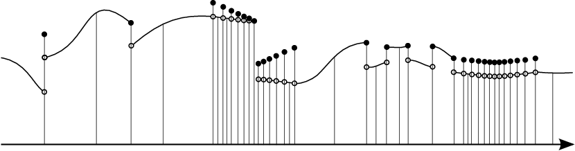
for each $x\in\mathbb{R}$ . Together with the points in $\mathbb{R}^{2}$ which are not in these segments (these points are the so-called singletons) this gives a decomposition of $\mathbb{R}^{2}$ . This has an interesting property: let $y\in[0,f(x)]$ for some $x\in\mathbb{R}$ and let $(x_{n})\in\mathbb{R}$ be a sequence (which is not necessarily convergent). If every nbhd of the point $(x,y)$ intersects all but finitely many segments $A_{x_{n}}$ , then the points $(u,v)\in\mathbb{R}^{2}$ each of whose nbhds intersects all but finitely many $A_{x_{n}}$ are in $A_{x}$ as well, see Figure 1. The set of the points $(u,v)$ is called the lower limit of the sequence $A_{x_{n}}$ . In other words, if an $A_{x}$ intersects the lower limit of a sequence $A_{x_{n}}$ , then all the lower limit is a subset of $A_{x}$ . More generally we have the following.

Refer to caption — Figure 1. The graph of an upper semi-continuous function $f$ and some segments $A_{x}$ . If the segments $A_{x_{n}}$ “converge” to a segment $A_{x}$ , then $f(x_{n})$ converges to a number $\leq f(x)$ .

Definition 2.5.

Let $A_{n}$ be a sequence of subsets of the space $X$ . The lower limit of $A_{n}$ is the set of the points $p\in X$ each of whose nbhds intersects all but finitely many $A_{n}$ . It is denoted by $\liminf A_{n}$ . The upper limit of $A_{n}$ is the set of the points $p\in X$ each of whose nbhds intersects infinitely many $A_{n}$ s. It is denoted by $\limsup A_{n}$ .

Note that $\liminf A_{n}\subset\limsup A_{n}$ is always true. In the previous example the sets $A_{x_{n}}$ could approach the set $A_{x}$ only in a manner determined by the function $f$ . This leads to the following general definition.

Definition 2.6.

Let $\mathcal{D}$ be a decomposition of a space $X$ such that all elements of $\mathcal{D}$ are closed and compact and they can converge to each other only in the following way: if $A\in\mathcal{D}$ , then for every nbhd $U$ of $A$ there is a nbhd $V$ of $A$ with the property $V\subset U$ such that if some element $B\in\mathcal{D}$ intersects $V$ , then $B\subset U$ , i.e. the set $B$ is completely inside the nbhd $U$ . Then $\mathcal{D}$ is an upper semi-continuous decomposition (usc decomposition for short). If all the decomposition elements are closed but not necessarily compact, then we say it is a closed upper semi-continuous decomposition.

For example, the decomposition defined in (2.1) is usc.

Lemma 2.7.

Let $\mathcal{D}$ be a decomposition of the space $X$ such that each decomposition element is closed. The following are equivalent:

(1)

$\mathcal{D}$ is a closed usc decomposition,
(2)

for every $D\in\mathcal{D}$ and every nbhd $U$ of $D$ there is a saturated nbhd $W\subset U$ of $D$ , that is an open set $W$ which is a union of decomposition elements,
(3)

for each open subset $U\subset X$ , the set $\cup\{D\in\mathcal{D}:D\subset U\}$ is open,
(4)

for each closed subset $F\subset X$ , the set $\cup\{D\in\mathcal{D}:D\cap F\neq\emptyset\}$ is closed,
(5)

the decomposition map $\pi\colon X\to X_{\mathcal{D}}$ is a closed map.

Proof.

Suppose $\mathcal{D}$ is usc and $U$ is a nbhd of $D$ . Let $W$ be the union of all decomposition elements which are subsets of $U$ . Then $D\subset W$ obviously and $W$ is open because if $x\in W$ , then $x\in D^{\prime}$ for some decomposition element $D^{\prime}\subset W$ and $D^{\prime}\subset U$ , so by definition $D^{\prime}\subset V\subset U$ for a nbhd $V$ but the nbhd $V$ of $x$ is in $W$ since all the decomposition elements intersecting $V$ have to be in $U$ , which means they are in $W$ as well. This shows that (1) implies (2). Suppose (2) holds. If $U$ is an open set, then for each decomposition element $D\subset U$ a saturated nbhd $W$ of $D$ is also in $U$ and also in $\cup\{D\in\mathcal{D}:D\subset U\}$ . This means that the set $\cup\{D\in\mathcal{D}:D\subset U\}$ is a union of open sets, which proves (3). We have that (3) and (4) are equivalent because we can take the complement of a given closed set $F$ or an open set $U$ . We have that (4) and (5) are equivalent: from (4) we can show (5) by taking an arbitrary closed set $F\subset X$ , then $\cup\{D\in\mathcal{D}:D\cap F\neq\emptyset\}$ is closed, its complement is a saturated open set whose $\pi$ -image is open so $\pi(F)$ is closed. If we suppose (5), then for a closed set $F\subset X$ the set

\pi^{-1}(\pi(F))=\cup\{D\in\mathcal{D}:D\cap F\neq\emptyset\}

is closed so we get (4). Finally (3) implies (1): if $D\in\mathcal{D}$ and $U$ is a nbhd of $D$ , then let $V$ be the open set $\cup\{D\in\mathcal{D}:D\subset U\}$ , this is a nbhd of $D$ , it is in $U$ and if a $D^{\prime}\in\mathcal{D}$ intersects $V$ , then it is in $V$ and hence also in $U$ . ∎

There is also the notion of lower semi-continuous decomposition: a decomposition $\mathcal{D}$ of a metric space is lower semi-continuous if for every element $A\in\mathcal{D}$ and for every $\varepsilon>0$ there is a nbhd $V$ of $A$ such that if some decomposition element $B$ intersects $V$ , then $A$ is in the $\varepsilon$ -nbhd of $B$ . A decomposition of a metric space is continuous if it is upper and lower semi-continuous, see Figure 2. We will not study decompositions which are only lower semi-continuous.

Theorem 2.8.

Let $X$ be a $T_{3}$ space and $\mathcal{D}$ is a closed usc decomposition. If $A_{n}\in\mathcal{D}$ is a sequence of decomposition elements and $A\in\mathcal{D}$ are such that $A\cap\liminf A_{n}\neq\emptyset$ , then $\limsup A_{n}\subset A$ .

Proof.

Suppose there is a point $x\in A$ such that $x\in\liminf A_{n}$ as well. By contradiction suppose that $\limsup A_{n}\nsubseteq A$ , this means that a point $y\in\limsup A_{n}$ is such that $y\notin A$ . Since $y\in D$ for a decomposition element, we get $D\neq A$ so $D$ is disjoint from the decomposition element $A$ . The space $X$ is $T_{3}$ , the sets $D$ and $\{x\}$ are closed so there is a nbhd $U$ of $D$ and a nbhd $V$ of $x$ which are disjoint from each other. We also have a nbhd $W\subset U$ of $D$ which is a union of decomposition elements by Lemma 2.7. Since $x\in\liminf A_{n}$ , we have that for an integer $k$ the sets $A_{k},A_{k+1},\ldots$ intersect $V$ . The nbhd $W$ is saturated, this implies that a decomposition element does not intersect both of $W$ and $V$ . So $A_{k},A_{k+1},\ldots$ are disjoint from $W$ . This contradicts to that $W$ is a nbhd of $y$ and so infinitely many $A_{n}$ has to intersect $W$ because $y\in\limsup A_{n}$ . ∎

An other example for a usc decomposition is the equivalence relation on $S^{n}$ defined by $x\sim-x$ . Here the decomposition elements are not connected and the decomposition space is the projective space ${\mathbb{R}}{P}^{n}$ . Or another example is the closed usc decomposition of $\mathbb{R}^{2}$ , where the two non-singleton decomposition elements are the two arcs of the graph of the function $x\mapsto 1/x$ , all the other decomposition elements are singletons. The decomposition space is homeomorphic to

A\cup_{\varphi}B\cup_{\psi}A^{\prime},

where $A$ and $A^{\prime}$ are open disks, each of them with one additional point in its frontier denoted by $a$ and $a^{\prime}$ respectively. The space $B$ is an open disk with two additional points $b,b^{\prime}$ in its frontier and the gluing homeomorphisms are $\varphi\colon\{a\}\to\{b\}$ and $\psi\colon\{a^{\prime}\}\to\{b^{\prime}\}$ . If a decomposition is given, then we would like to understand the decomposition space as well.

Proposition 2.9.

The decomposition space of a closed usc decomposition of a normal space is $T_{4}$ .

Proof.

We have to show that if $\mathcal{D}$ is a usc decomposition of a normal space $X$ , then any two disjoint closed sets in the space $X_{\mathcal{D}}$ can be separated by open sets. Let $A,B$ be disjoint closed sets in $X_{\mathcal{D}}$ . Then $\pi^{-1}(A)$ and $\pi^{-1}(B)$ are disjoint closed sets and by being $X$ normal and by Lemma 2.7 they have disjoint saturated nbhds $U_{1}$ and $U_{2}$ . Taking $\pi(U_{1})$ and $\pi(U_{2})$ we get disjoint nbhds of $A$ and $B$ . The decomposition elements are closed so $X_{\mathcal{D}}$ is $T_{1}$ , which finally implies that $X_{\mathcal{D}}$ is $T_{4}$ . ∎

If a space $X$ is not normal, then it is easy to define such closed usc decomposition, where the decomposition space is even not $T_{2}$ . Take two disjoint closed sets $A,B$ in $X$ which can not be separated by open sets. For example the direct product of the Sorgenfrei line with itself is not normal and choose the points with rational and irrational coordinates in the antidiagonal respectively, to have two closed sets $A$ and $B$ . These two sets are the two non-singleton elements of the decomposition $\mathcal{D}$ , other elements are singletons. Then $\mathcal{D}$ is closed usc but $X_{\mathcal{D}}$ is not $T_{2}$ because $\pi(A)$ and $\pi(B)$ can not be separated by open sets.

Definition 2.10.

Let $\mathcal{D}$ be a decomposition of the space $X$ . A decomposition is finite if it has only finitely many non-degenerate elements and countable if it has countably many non-degenerate elements. A decomposition is monotone if every decomposition element is connected. If $X$ is a metric space, then a decomposition is null if the decomposition elements are bounded and for every $\varepsilon>0$ there is only a finite number of elements whose diameter is greater than $\varepsilon$ .

Proposition 2.11.

Let $\mathcal{D}$ be a decomposition and suppose that all elements are closed. If $\mathcal{D}$ is finite, then it is a closed usc decomposition.

Proof.

Let $C\subset X$ be a closed subset, then $\pi^{-1}(\pi(C))$ is closed because it is the finite union of the closed set $C$ and the non-degenerate elements which intersect $C$ . Then by Lemma 2.7 (4) the statement follows. ∎

Proposition 2.12.

If $\mathcal{D}$ is a closed and null decomposition of a metric space, then it is usc.

Proof.

Denote the metric by $d$ . All the decomposition elements are compact because they are bounded. Let $U$ be a nbhd of a $D\in\mathcal{D}$ , then there is an $\varepsilon>0$ such that the $\varepsilon$ -nbhd of $D$ is in $U$ . Since $\mathcal{D}$ is null, there are only finitely many decomposition elements $D_{1},\ldots,D_{n}$ whose diameter is greater than $\varepsilon/4$ and $D_{i}\neq D$ . Let $\delta$ be the minimum of $\varepsilon/4$ and the distances between $D$ and the $D_{i}$ s. If $D^{\prime}\in\mathcal{D}$ is such that the distance between $D^{\prime}$ and $D$ is less than $\delta$ , then $D^{\prime}$ is in the $\varepsilon$ -nbhd of $D$ : there are $x\in D$ and $y\in D^{\prime}$ such that $d(x,y)<\delta$ so for every $a\in D^{\prime}$

\inf\{d(a,b):b\in D\}\leq d(a,y)+d(y,x)+\inf\{d(x,b):b\in D\}=d(a,y)+d(y,x)\leq\\ {\mathrm{diam}}\thinspace D^{\prime}+\delta\leq\varepsilon/2,

which means that $D^{\prime}$ is in the $\varepsilon$ -nbhd of $D$ so $D^{\prime}\subset U$ . ∎

Proposition 2.13.

Let $\mathcal{D}$ be a usc decomposition of a space $X$ .

(1)

If $X$ is $T_{2}$ , then $X_{\mathcal{D}}$ is $T_{2}$ as well.
(2)

If $X$ is regular, then $X_{\mathcal{D}}$ is $T_{3}$ .

Proof.

The decomposition elements are compact so every $\pi^{-1}(a)$ and $\pi^{-1}(b)$ for different $a,b\in X_{\mathcal{D}}$ can be separated by open sets. The statement follows easily. ∎

Proposition 2.14.

Let $\mathcal{D}$ be a usc decomposition of a $T_{2}$ space $X$ . The decomposition $\mathcal{D}^{\prime}$ whose elements are the connected components of the elements of $\mathcal{D}$ is a monotone usc decomposition.

Proof.

Take an element $D^{\prime}\in\mathcal{D}^{\prime}$ and denote by $D$ the decomposition element in $\mathcal{D}$ which contains $D^{\prime}$ . Suppose $D\neq D^{\prime}$ . Then $D-D^{\prime}$ is closed in $D$ so it is closed in $X$ . Let $U$ be a nbhd of $D^{\prime}$ . Then there exists a nbhd $U^{\prime}\subset U$ of $D^{\prime}$ which is disjoint from a nbhd $U^{\prime\prime}$ of the closed set $D-D^{\prime}$ . By the usc property we can find a nbhd $V$ of $D$ such that $V\subset U^{\prime}\cup U^{\prime\prime}$ and if a $C\in\mathcal{D}$ intersects $V$ , then $C\subset U^{\prime}\cup U^{\prime\prime}$ . If $C^{\prime}\in\mathcal{D}^{\prime}$ intersects $V\cap U^{\prime}$ , then the element $C\in\mathcal{D}$ which contains $C^{\prime}$ as a connected component intersects $V$ hence $C\subset U^{\prime}\cup U^{\prime\prime}$ . Since $U^{\prime}$ and $U^{\prime\prime}$ are disjoint, the component $C^{\prime}$ of $C$ is in $U^{\prime}$ because it intersects $U^{\prime}$ . We got that $C^{\prime}\subset U$ . ∎

For example, it follows that the decomposition of a compact $T_{2}$ space $X$ whose elements are the connected components of the space is a usc decomposition. To see this, at first take the decomposition $\mathcal{D}$ , where $\mathcal{H}_{\mathcal{D}}=\{X\}$ and hence the decomposition has no singletons. This is usc so we can apply the previous proposition.

Proposition 2.15.

If $X$ is a metric space and $\mathcal{D}$ is its usc decomposition, then $X_{\mathcal{D}}$ is metrizable. If $X$ is separable, then $X_{\mathcal{D}}$ is also separable.

Proof.

By [St56] if there is a continuous closed map $f$ of a metric space onto a space $Y$ such that for every $y\in Y$ the closed set $f^{-1}(y)-{\mathrm{int}}\thinspace f^{-1}(y)$ is compact, then $Y$ is metrizable. But for every $y\in X_{\mathcal{D}}$ the set $\pi^{-1}(y)$ and so its closed subset $\pi^{-1}(y)-{\mathrm{int}}\thinspace\pi^{-1}(y)$ are compact hence $X_{\mathcal{D}}$ is metrizable. Moreover if $X$ is separable, then there is a countable subset $S\subset X$ intersecting every open set, which gives the countable set $\pi(S)$ intersecting every open set in $X_{\mathcal{D}}$ . ∎

3. Examples and properties of decompositions

Usually, we are interested in the topology of the decomposition space if a decomposition of $X$ is given. Especially those situations are stimulating where the decomposition space turns out to be homeomorphic to $X$ .

Let $X=\mathbb{R}$ and let $\mathcal{D}$ be a decomposition such that $\mathcal{H}_{\mathcal{D}}$ consists of countably many disjoint compact intervals. Then this is a usc decomposition: any open interval $U\subset\mathbb{R}$ contains at most countably many compact intervals of $\mathcal{H}_{\mathcal{D}}$ and the infimum of the left endpoints of these intervals could be in $U$ or it could be the left boundary point of $U$ . Similarly, we have this for the right endpoints. In all cases the union of the decomposition elements being in $U$ is open. For an arbitrary open set $U\subset\mathbb{R}$ we have the same, this means we have a usc decomposition. Later we will see, that the decomposition space $X_{\mathcal{D}}$ is homeomorphic to $\mathbb{R}$ . Moreover the decomposition map $\pi\colon X\to X_{\mathcal{D}}$ is approximable by homeomorphisms, which means there are homeomorphisms from $\mathbb{R}$ to $\mathbb{R}$ arbitrarily close to $\pi$ in the sense of uniform metric. For example, let $X=\mathbb{R}$ and consider the infinite Cantor set-like construction by taking iteratively the middle third compact intervals in the interval $[0,1]$ . These are countably many intervals and define the decomposition ${\mathcal{D}}$ so that the non-degenerate elements are these intervals. We can obtain this decomposition ${\mathcal{D}}$ by taking the connected components of $[0,1]-\mbox{Cantor set}$ and then taking the closure of them. This is usc and we will see that the decomposition space is $\mathbb{R}$ .

If $X=\mathbb{R}^{2}$ , then an analogous decomposition is that $\mathcal{H}_{\mathcal{D}}$ consists of countably many compact line segments. More generally, let $\mathcal{H}_{\mathcal{D}}$ be countably many flat arcs, that is such subsets $A$ of $\mathbb{R}^{2}$ for which there exist self-homeomorphisms $h_{A}$ of $\mathbb{R}^{2}$ mapping $A$ into the standard compact interval $\{(x,0)\in\mathbb{R}^{2}:0\leq x\leq 1\}$ . Such a decomposition is not necessarily usc, for example take the function $f\colon[0,1)\to\mathbb{R}$ , $f(x)=1+x$ , and the sequence $x_{n}=1-1/n$ . Define the decomposition by $\mathcal{H}_{\mathcal{D}}=\{(x_{n},y):y\in[0,f(x_{n})],n\in\mathbb{N}\}$ and the singletons are all the other points of $\mathbb{R}^{2}$ . Then $\mathcal{H}_{\mathcal{D}}$ consists of countably many straight line segments but this decomposition is not usc: consider the point $(1,3/2)\in\mathcal{D}$ and its $\varepsilon$ -nbhds for small $\varepsilon>0$ . These intersect infinitely many non-degenerate decomposition elements but none of the elements is a subset of any of these $\varepsilon$ -nbhds. The decomposition space is not $T_{2}$ : the points $\pi((1,y))$ , where $0\leq y\leq 2$ , cannot be separated by disjoint nbhds because the sequence $\pi((x_{n},0))$ converges to all of them.

However, if $\mathcal{D}$ is such a decomposition of $\mathbb{R}^{2}$ that $\mathcal{H}_{\mathcal{D}}$ consists of countably many flat arcs and further we suppose that $\mathcal{D}$ is usc, then the decomposition space $X_{\mathcal{D}}$ is homeomorphic to $\mathbb{R}^{2}$ and again $\pi$ can be approximated by homeomorphisms, we will see this later.

We get another interesting example by taking a smooth function with finitely many critical values on a closed manifold $M$ . Then the decomposition elements are defined to be the connected components of the point preimages of the function. This is a monotone decomposition ${\mathcal{D}}$ and it is usc because the decomposition map $\pi\colon M\to M_{\mathcal{D}}$ is a closed map: in $M$ a closed set is compact, its $\pi$ -image is compact as well and $M_{\mathcal{D}}$ is $T_{2}$ because it is a graph [Iz88, Re46, Sa20] so this $\pi$ -image is also closed.

If $X$ is $3$ -dimensional, then the possibilites increase tremendously. This is illustrated by the following surprising statement.

Proposition 3.1.

For every compact metric space $Y$ there exists a monotone usc decomposition of the compact ball $D^{3}$ such that $Y$ can be embedded into the decomposition space.

Proof.

Recall that by the Alexandroff-Hausdorff theorem the Cantor set in the $[0,1]$ interval can be mapped surjectively and continuously onto every compact metric space. Let $T$ be a tetrahedron in $D^{3}$ , denote two of its non-intersecting edges by $e$ and $f$ . Identify these edges linearly with $[0,1]$ and let $C_{1}$ and $C_{2}$ be the Cantor sets in $e$ and $f$ , respectively. For $i=1,2$ denote the existing surjective maps of $C_{i}$ onto $Y$ by $\psi_{i}\colon C_{i}\to Y$ . For every $x\in Y$ take the union of all the line segments in $T$ connecting all the points of $\psi_{1}^{-1}(x)$ to all the points of $\psi_{2}^{-1}(x)$ . Denote this subset of $T$ by $D_{x}$ , see Figure 3. They are compact and connected for all $x\in Y$ and they are pairwise disjoint because all the lines in $T$ connecting points of $e$ and $f$ are pairwise disjoint. So we have a monotone usc decomposition with $\mathcal{H}_{\mathcal{D}}=\{D_{x}:x\in Y\}$ . Define the embedding $i$ of $Y$ into $D^{3}_{\mathcal{D}}$ by $i(x)=\pi(\psi_{1}^{-1}(x))$ . This map is injective, closed because $\pi$ is closed and continuous because $\psi_{1}$ is closed. ∎

To see further examples in $\mathbb{R}^{3}$ let us introduce some notions.

Definition 3.2 (Defining sequence).

Let $X$ be a connected $n$ -dimensional manifold. A defining sequence for a decomposition of $X$ is a sequence

C_{1},C_{2},\ldots,C_{n},\ldots

of compact $n$ -dimensional submanifolds-with-boundary in $X$ such that $C_{n+1}\subset\mathrm{int}\thinspace C_{n}$ . The decomposition elements of the defined decomposition are the connected components of $\cap_{n=1}^{\infty}C_{n}$ and the other points of $X$ are singletons.

Obviously a decomposition defined in this way is monotone. The set $\cap_{n=1}^{\infty}C_{n}$ is closed and compact so its connected components are closed and compact as well. Also the space $\cap_{n=1}^{\infty}C_{n}$ is $T_{2}$ hence its decomposition to its connected components is usc. Then adding all the points of $X-\cap_{n=1}^{\infty}C_{n}$ to this decomposition as singletons results our decomposition. This is usc: the only thing which is not completely obvious is that in a nbhd of an added point the conditions being usc are satisfied or not. But $\cap_{n=1}^{\infty}C_{n}$ is closed, its complement is open so every such singleton has a nbhd disjoint from $\cap_{n=1}^{\infty}C_{n}$ .

Proposition 3.3.

If all $C_{n}$ in a defining sequence is connected, then $\cap_{n=1}^{\infty}C_{n}$ is connected.

Proof.

Let $C$ denote the non-empty set $\cap_{n=1}^{\infty}C_{n}$ . Suppose $C$ is not connected, this means there are disjoint closed non-empty subsets $A,B\subset C$ such that $A\cup B=C$ . These $A$ and $B$ are closed in the ambient manifold $X$ as well, so there exist disjoint nbhds $U$ of $A$ and $V$ of $B$ in $X$ . It is enough to show that for some $n\in\mathbb{N}$ we have $C_{n}\subset U\cup V$ , because then $C_{n}\cap U\neq\emptyset$ , $C_{n}\cap V\neq\emptyset$ imply that $C_{n}$ is not connected, which is a contradiction. If we suppose that for every $n\in\mathbb{N}$ we have $C_{n}\cap(X-(U\cup V))\neq\emptyset$ , then for every $n$ we have $C_{n}\cap(X-U)\cap(X-V)\neq\emptyset$ , i.e. the closed set $F=(X-U)\cap(X-V)$ and each element of the nested sequence $C_{1},C_{2},\ldots$ satisfy

C_{n}\cap F\neq\emptyset.

Of course

C_{n+1}\cap F\subset C_{n}\cap F

which implies that

F\cap C=F\cap(\cap_{n=1}^{\infty}C_{n})=\cap_{n=1}^{\infty}(C_{n}\cap F)\neq\emptyset

because all $C_{n}\cap F$ is closed in the compact space $C_{1}$ . But $F\cap C\neq\emptyset$ contradicts to $C\subset U\cup V$ . ∎

The $\pi$ -image of the union of non-degenerate elements of a decomposition associated to a defining sequence is closed and also totally disconnected because if $\cap_{n=1}^{\infty}C_{n}$ is not connected, then all the pairs of decomposition elements have disjoint saturated nbhds which yield disjoint nbhds of their $\pi$ -image.

3.1. The Whitehead continuum

One of the most famous such decomposition is related to the so called Whitehead continuum. Its defining sequence consists of solid tori embedded into each other in such a way that $C_{i+1}$ is a thickened Whitehead double of the center circle of $C_{i}$ , see Figure 4. The intersection $\cap_{i=1}^{\infty}C_{i}$ is a compact subset of $\mathbb{R}^{3}$ , this is the Whitehead continuum, which we denote by $\mathcal{W}$ . The decomposition consists of the connected components of $\mathcal{W}$ and the singletons in the complement of them. If the diameters $d_{i}$ of the meridians of the tori $C_{i}$ converges to $0$ as $i$ goes to $\infty$ , then $\mathcal{W}$ intersects the vertical sheet $S$ in Figure 4 in a Cantor set: $C_{i}\cap S$ is equal to $2^{i-1}$ copies of disks of diameter $d_{i}$ nested into each other. The intersection $S\cap(\cap_{i=1}^{\infty}C_{i})$ is then a Cantor set. The Whitehead continuum $\mathcal{W}$ is connected because the $C_{i}$ tori are connected but it is not path-connected. We will see later that the decomposition space $\mathbb{R}^{3}_{\mathcal{W}}$ is not homeomorphic to $\mathbb{R}^{3}$ but taking its direct product with $\mathbb{R}$ we get $\mathbb{R}^{4}$ . An important property of $\mathbb{R}^{3}-\mathcal{W}$ is that it is a contractible $3$ -manifold, which is not homeomorphic to $\mathbb{R}^{3}$ .

For understanding further properties of this decomposition, we are going to define some notions.

Definition 3.4 (Cellular set, cell-like set).

Let $X$ be an $n$ -dimensional manifold and $C\subset X$ be a subset of $X$ . The set $C$ is cellular if there is a sequence $B_{1},B_{2},\ldots,B_{n},\ldots$ of closed $n$ -dimensional balls in $X$ such that $B_{n+1}\subset\mathrm{int}\thinspace B_{n}$ and $C=\cap_{n=1}^{\infty}B_{n}$ . A compact subset $C$ of a topological space $X$ is cell-like if for every nbhd $U$ of $C$ there is a nbhd $V$ of $C$ in $U$ such that the inclusion map $V\to U$ is homotopic in $U$ to a constant map. Similarly, a decomposition is called cellular or cell-like if each of its decomposition elements is cellular or cell-like, respectively.

For example the “topologist’s sine curve” in $\mathbb{R}^{2}$ is cellular. A cellular set is compact and also connected but not necessarily path-connected. It is also easy to see that every compact contractible subset of a manifold is cell-like. Also a compact and contractible metric space is cell-like in itself. A cell-like set $C$ is connected because if there were two open subsets $U_{1}$ and $U_{2}$ in $X$ separating some connected components of $C$ , then it would be not possible to contract any nbhd $V\subset U_{1}\cup U_{2}$ of $C$ to one single point.

Proposition 3.5.

The set $\mathcal{W}$ is cell-like but not cellular.

Proof.

Let $U$ be a nbhd of $\mathcal{W}$ . Then there is an $n$ such that $C_{i}\subset U$ for all $i\geq n$ . Let $V$ be such a small tubular nbhd of $C_{n+1}$ which is inside $C_{n}$ . Then since the Whitehead double of the center circle of $C_{n}$ is null-homotopic in the solid torus $C_{n}$ , the thickened Whitehead double $C_{n+1}$ and its nbhd $V$ are also null-homotopic in $C_{n}$ , hence the map $V\to U$ is homotopic in $U$ to a constant map.

Lemma 3.6.

The $3$ -manifold $S^{3}-\mathcal{W}$ is not simply connected at infinity.

Proof.

We have to show that there is a compact subset $C\subset S^{3}-\mathcal{W}$ such that for every compact set $D\subset S^{3}-\mathcal{W}$ containing $C$ the induced homomorphism

\varphi\colon\pi_{1}(S^{3}-\mathcal{W}-D)\to\pi_{1}(S^{3}-\mathcal{W}-C)

is not the zero homomorphism. Let $C$ be the closure of $S^{3}-C_{1}$ . If $D$ is a compact set in $S^{3}-\mathcal{W}$ containing $C$ , then $S^{3}-D$ is a nbhd of $\mathcal{W}$ in $C_{1}$ . Then there is an $n$ such that $C_{i}\subset S^{3}-D$ for all $i\geq n$ . Consider the commutative diagram

\begin{CD}\pi_{1}(S^{3}-C_{n}-D)@>{}>{}>\pi_{1}(S^{3}-C_{n}-C)\\ @V{}V{}V@V{}V{\alpha}V\\ \pi_{1}(S^{3}-\mathcal{W}-D)@>{\varphi}>{}>\pi_{1}(S^{3}-\mathcal{W}-C).\end{CD}

By [NW37] the generator of the group $\pi_{1}(S^{3}-C_{n}-C)$ represented by the meridian of the torus $C_{n}$ is mapped by $\alpha$ into a generator of $\pi_{1}(S^{3}-\mathcal{W}-C)$ . Since this meridian also represents an element of $\pi_{1}(S^{3}-C_{n}-D)$ , we get that $\varphi$ is not the zero homomorphism. ∎

Let us continue the proof of Proposition 3.5. If $\mathcal{W}$ is cellular, then there are $B_{1},B_{2},\ldots,B_{n},\ldots$ closed $n$ -dimensional balls in $S^{3}$ such that $B_{n+1}\subset\mathrm{int}\thinspace B_{n}$ and $\mathcal{W}=\cap_{n=1}^{\infty}B_{n}$ . This would imply that $S^{3}-\mathcal{W}$ is simply connected at infinity because if $C\subset S^{3}-\mathcal{W}$ is a compact set, then take a $B_{n}\subset S^{3}-C$ and a loop in $\mathrm{int}B_{n}-\mathcal{W}$ , then there is a $B_{m}\subset\mathrm{int}B_{n}$ not containing this loop and the loop in null-homotopic in $\mathrm{int}B_{n}-B_{m}$ because $\pi_{1}(\mathrm{int}B_{n}-B_{m})=0$ . Hence we obtain that $S^{3}-\mathcal{W}$ is not cellular. ∎

With more effort we could show that $S^{3}-\mathcal{W}$ is contractible so it is homotopy equivalent to $\mathbb{R}^{3}$ but by the previous statement it is not homeomorphic to $\mathbb{R}^{3}$ . It is known that the set $\mathcal{W}\times\{0\}$ is cellular in $\mathbb{R}^{3}\times\mathbb{R}$ and the decomposition space of the decomposition of $\mathbb{R}^{3}\times\mathbb{R}$ whose only non-degenerate element is $\mathcal{W}\times\{0\}$ is homeomorphic to $\mathbb{R}^{4}$ . This fact is the starting point of the proof of the $4$ -dimensional Poincaré conjecture.

Being cell-like often does not depend on the ambient space. To understand this, we have to introduce a new notion.

Definition 3.7 (Absolute nbhd retract).

A metric space $Y$ is an absolute nbhd retract (or ANR for short) if for an arbitrary metric space $X$ and its closed subset $A$ every map $f$ from $A$ to $Y$ extends to a nbhd of $A$ . In other words, the nbhd $U$ and the dashed arrow exist in the following diagram and make the diagram commutative.

This is equivalent to say that for every metric space $Z$ and embedding $i\colon Y\to Z$ such that $i(Y)$ is closed there is a nbhd $U$ of $i(Y)$ in $Z$ which retracts onto $i(Y)$ , that is $r|_{i(Y)}=\mathrm{id}_{i(Y)}$ for some map $r\colon U\to i(Y)$ . It is a fact that every manifold is an ANR.

The property of cell-likeness is independent of the ambient space until that is an ANR as the following statement shows.

Proposition 3.8.

If $C\subset X$ is a compact cell-like set in a metric space $X$ , then the embedded image of $C$ in an arbitrary ANR is also cell-like.

Proof.

Suppose $e\colon C\to Y$ is an embedding into an ANR $Y$ . We have to show that $e(C)$ is cell-like. Let $U$ be a nbhd of $e(C)$ . Since $Y$ is ANR, there is a nbhd $\tilde{V}$ of $C$ in $X$ such that $e$ extends to an $\tilde{e}\colon\tilde{V}\to Y$ . Let $V\subset X$ be the open set $\tilde{V}\cap\tilde{e}^{-1}(U)$ , it is a nbhd of $C$ . There is a nbhd $W$ of $C$ such that $C\subset W\subset V$ and there is a homotopy of the inclusion $W\subset V$ to the constant in $V$ since $C$ is cell-like, denote this homotopy by $\varphi\colon W\times[0,1]\to V$ . Then $\varphi|_{C\times[0,1]}$ is a homotopy of the inclusion $C\subset V$ to the constant. Take

\tilde{e}\circ\varphi|_{C\times[0,1]}\circ(e^{-1}|_{e(C)}\times\mathrm{id}_{[0,1]}),

this is a homotopy of the inclusion $e(C)\subset U$ to the constant in $U$ . The space $e(C)\times[0,1]$ is compact in $Y\times[0,1]$ and the homotopy maps it into $Y$ , which is ANR. This implies that there is a nbhd $\tilde{U}\subset U$ of $e(C)$ such that the inclusion $\tilde{U}\subset U$ is homotopic to constant in $U$ . ∎

For example, this shows that a compact and contractible metric space is cell-like if we embed it into any ANR. In practice, we do not consider cell-like sets as subsets in some ambient space but rather as compact metric spaces which are cell-like if we embed them into an arbitrary ANR.

It is clear that every cellular set $C$ is cell-like because in every nbhd $U$ of $C$ some open ball is contractible. Also, we have seen that the Whitehead continuum is cell-like but not cellular. In order to compare cell-like and cellular sets we introduce the notion of cellularity criterion.

Definition 3.9 (Cellularity criterion).

A subset $Y\subset X$ satisfies the cellularity criterion if for every nbhd $U$ of $Y$ there is a nbhd $V$ of $Y$ such that $V\subset U$ and every loop in $V-Y$ is null-homotopic in $U-Y$ .

The cellularity criterion and being cellular measure how wildly a subset is embedded into a space. The next theorem compares cell-like and cellular sets in a PL manifold. We omit its difficult proof here.

Theorem 3.10.

Let $C$ be a cell-like subset of a PL $n$ -dimensional manifold, where $n\geq 4$ . Then $C$ is cellular if and only if $C$ satisfies the cellularity criterion.

In dimension $2$ we have a simpler statement:

Theorem 3.11.

Every cell-like subset in a $2$ -dimensional manifold $X$ is cellular.

Proof.

At first suppose $X=\mathbb{R}^{2}$ and $C\subset\mathbb{R}^{2}$ is a cell-like set. Let $U$ be a bounded nbhd of $C$ and let $V\subset U$ a nbhd of $C$ such that the inclusion $V\to U$ is homotopic to constant. Choose another nbhd $W\subset V$ of $C$ as well such that $\mathrm{cl}\thinspace W\subset V$ . Take a compact smooth $2$ -dimensional manifold $H\subset V$ such that $C\subset\mathrm{int}H$ , $\partial H\subset V-\mathrm{cl}\thinspace W$ and $\mathrm{int}H$ is connected. Such an $H$ can be obtained by taking a Morse function $f\colon V\to[0,1]$ which maps the nbhd $W$ of $C$ into $0$ and a small nbhd of $\mathbb{R}^{2}-V$ into $1$ . Then the preimage of a regular value $r$ close to $1/2$ is a smooth $1$ -dimensional submanifold of $\mathbb{R}^{2}$ and the preimage of $(-\infty,r]$ is a compact subset containing $W$ and $C$ , denote this $f^{-1}((-\infty,r])$ by $H$ . Then $H$ is a compact smooth $2$ -dimensional submanifold of $\mathbb{R}^{2}$ , see Figure 5. Take its connected component (this is also a path-connected component because $H$ is a manifold) which contains $C$ and denote this by $H$ as well.

We show that $H-C$ is connected. For this consider the commutative diagram

\begin{CD}H_{1}(H;\mathbb{Z}_{2})@>{}>{}>H_{1}(H,H-C;\mathbb{Z}_{2})@>{}>{}>H_{0}(H-C;\mathbb{Z}_{2})@>{}>{}>H_{0}(H)@>{}>{}>0\\ @V{}V{}V@V{}V{}V@V{}V{}V@V{}V{}V\\ H_{1}(\mathbb{R}^{2};\mathbb{Z}_{2})@>{}>{}>H_{1}(\mathbb{R}^{2},\mathbb{R}^{2}-C;\mathbb{Z}_{2})@>{}>{}>H_{0}(\mathbb{R}^{2}-C;\mathbb{Z}_{2})@>{i_{*}}>{}>H_{0}(\mathbb{R}^{2})@>{}>{}>0\end{CD}

coming from the long exact sequences and the inclusion $(H,H-C)\subset(\mathbb{R}^{2},\mathbb{R}^{2}-C)$ . This is just the diagram

\begin{CD}H_{1}(H;\mathbb{Z}_{2})@>{}>{}>H_{1}(H,H-C;\mathbb{Z}_{2})@>{}>{}>H_{0}(H-C;\mathbb{Z}_{2})@>{}>{}>\mathbb{Z}_{2}@>{}>{}>0\\ @V{}V{}V@V{}V{\cong}V@V{}V{}V@V{}V{\cong}V\\ 0@>{}>{}>H_{1}(\mathbb{R}^{2},\mathbb{R}^{2}-C;\mathbb{Z}_{2})@>{}>{}>H_{0}(\mathbb{R}^{2}-C;\mathbb{Z}_{2})@>{i_{*}}>{}>\mathbb{Z}_{2}@>{}>{}>0\end{CD}

If the group $H_{0}(\mathbb{R}^{2}-C;\mathbb{Z}_{2})$ is $\mathbb{Z}_{2}$ , i.e. the manifold $\mathbb{R}^{2}-C$ is connected, then exactness implies that $H_{0}(H-C;\mathbb{Z}_{2})\cong\mathbb{Z}_{2}$ so $H-C$ is connected. To show that $\mathbb{R}^{2}-C$ is connected, we apply [HW41, Theorem VI.5, page 86], which implies that if $C$ is a closed subset of a space $D$ and $f,g$ are homotopic maps of $C$ into $S^{1}$ such that $f$ extends to $D$ , then $g$ extends to $D$ and the extensions are homotopic. Suppose the open set $\mathbb{R}^{2}-C$ is not connected, then it is the disjoint union of two open sets $A$ and $B$ . At least one of these is bounded because for large enough $s$ the set $\mathbb{R}^{2}-[-s,s]^{2}$ is disjoint from $C$ and it is connected hence it is in $A$ or $B$ but then $[-s,s]^{2}$ contains $B$ or $A$ , respectively. Suppose $A$ is bounded, $p\in A$ and $q\in B$ . For a subset $S\subset\mathbb{R}^{2}$ and point $x\in\mathbb{R}^{2}$ denote by $\pi_{S,x}\colon S-\{x\}\to S^{1}$ the radial projection of $S-\{x\}$ to the circle $S^{1}$ of radius $1$ centered at $x$ . Then $\pi_{C,q}$ extends to $\mathbb{R}^{2}-\{q\}$ so also to $A\cup C$ but $\pi_{C,p}$ does not extend to $A\cup C$ because such an extension would extend to a much larger disk $P$ centered at $p$ as well by radial projection and then a retraction of $P$ onto its boundary (if we identify it with the target circle of $\pi_{C,p}$ ) would exists. Consequently $\pi_{C,q}$ and $\pi_{C,p}$ are not homotopic and so at least one of them is not homotopic to constant. This means if $\mathbb{R}^{2}-C$ is not connected, then there is a map $C\to S^{1}$ which is not homotopic to constant. But since the inclusion $V\subset U$ and then also $C\subset U$ are homotopic to constant, we get that $\mathbb{R}^{2}-C$ is connected.

Finally, we get that $H-C$ is a path-connected smooth $2$ -dimensional manifold with boundary. Hence if the number of components of $\partial H$ is larger than one, then there exists a smooth curve transversal to $\partial H$ , disjoint from $C$ and connecting different components of $\partial H$ . We can cut $H$ along this curve and by repeating this process we end up with $\partial H$ being a single circle. By the Jordan curve theorem $H$ is a compact $2$ -dimensional disk. In this way we get

C\subset W\subset\mathrm{int}H\subset H\subset V\subset U.

Since in $\mathbb{R}^{2}$ every compact set is a countable intersection of open sets which form a decreasing sequence, we have $C=\cap_{n=1}^{\infty}U_{n}$ , where $U_{1}\supset U_{2}\supset\cdots\supset U_{n}\supset\cdots$ , where the sets $U_{n}$ are open. We can also assume that for each $n$ we have $\mathrm{cl}\thinspace U_{n+1}\subset U_{n}$ .

We obtain countably many compact $2$ -dimensional disks $H_{1},H_{2},\ldots$ by the previous construction, which satisfy

C\subset U_{n+1}\subset\mathrm{int}H_{n}\subset H_{n}\subset V\subset U_{n}.

Hence $C=\cap_{n=1}^{\infty}H_{n}$ so $C$ is cellular.

In the case of $X$ is an arbitrary $2$ -dimensional manifold, since $C$ is cell-like, there exists a nbhd of $C$ which is homotopic to constant so $C$ is contained in a simply-connected $2$ -dimensional manifold nbhd, which is homeomorphic to $\mathbb{R}^{2}$ . Hence a similar argument gives that $C$ is cellular. ∎

Proposition 3.12.

If $C$ is cell-like in a smooth $n$ -dimensional manifold $X$ , where $n\geq 3$ , then $C\times\{0\}$ is cellular in $X\times\mathbb{R}^{3}$ .

Proof.

It is enough to show that $C\times\{0\}$ satisfies the cellularity criterion. It is easy to see that $C\times\{0\}$ is cell-like in $X\times\mathbb{R}^{3}$ . Let $U$ be a nbhd of $C\times\{0\}$ in $X\times\mathbb{R}^{3}$ . It is obvious that there is a nbhd $V\subset U$ of $C\times\{0\}$ such that every loop $\gamma\colon[0,1]\to V$ is null-homotopic in $U$ . Let $\gamma$ be an arbitrary loop in $V-C\times\{0\}$ , it is homotopic to a smooth loop in $\tilde{\gamma}\colon V-C\times\{0\}$ by a homotopy $H$ . A homotopy of $\tilde{\gamma}$ to constant can be approximated by a smooth map $\tilde{H}\colon D^{2}\to U$ , where $\tilde{H}|_{\partial D^{2}}=\tilde{\gamma}$ . In the subspace $X\times\{0\}$ of $X\times\mathbb{R}^{3}$ let $W$ be a nbhd of $C\times\{0\}$ which is disjoint from the homotopy $\tilde{H}$ . Perturb $\tilde{H}$ keeping $\tilde{H}|_{\partial D^{2}}$ fixed to get a transversal map to the $n$ -dimensional manifold $W$ in $U$ , hence we get that $\gamma$ is null-homotopic in $U-C\times\{0\}$ . So the cellularity criterion holds for $C\times\{0\}$ . ∎

3.2. Antoine’s necklace

Take the defining sequence where

•

$C_{1}$ is a solid torus,
•

$C_{2}$ is a finite number of solid tori embedded in $C_{1}$ in such a way that each torus is unknotted and linked to its neighbour as in a usual chain,
•

$C_{3}$ is again a finite number of similarly linked solid tori,

…, etc., see Figure 6.

We always consider at least three tori in each $C_{n}$ . We require that the maximal diameter of tori in $C_{n}$ converges to $0$ . The set $\cap_{n=1}^{\infty}C_{n}$ is called Antoine’s necklace and denoted by $\mathcal{A}$ . It is easy to see that each of its components is cell-like. Unlike Whitehead continuum the components of $\mathcal{A}$ are cellular because every component of $C_{n+1}$ is inside a ball in $C_{n}$ .

Recall that the Cantor set is the topological space

D_{1}\times D_{2}\times\cdots\times D_{n}\times\cdots,

where every space $D_{n}$ is a finite discrete metric space with $|D_{n}|\geq 2$ .

Proposition 3.13.

The space $\cap_{n=1}^{\infty}C_{n}$ is homeomorphic to the Cantor set.

Proof.

Denote the number of tori embedded in $C_{1}$ by $m_{1}$ , these tori are

C_{2,1},\ldots,C_{2,m_{1}}

whose disjoint union is $C_{2}$ . For $1\leq i_{1}\leq m_{1}$ take the $i_{1}$ -th torus $C_{2,i_{1}}$ and denote the number of tori embedded into it by $m_{2,i_{1}}$ , these tori are

C_{3,i_{1},1},\ldots,C_{3,i_{1},m_{2,i_{1}}}

whose disjoint union is $C_{3}$ . Again for $1\leq i_{2}\leq m_{2,i_{1}}$ take the $i_{2}$ -th torus $C_{3,i_{1},i_{2}}$ and denote the number of tori embedded into it by $m_{3,i_{1},i_{2}}$ , these tori are

C_{4,i_{1},i_{2},1},\ldots,C_{4,i_{1},i_{2},m_{3,i_{1},i_{2}}}

whose disjoint union is $C_{4}$ . In general in the $n$ -th step for $1\leq i_{n}\leq m_{n,i_{1},\ldots,i_{n-1}}$ take the $i_{n}$ -th torus $C_{n+1,i_{1},\ldots,i_{n}}$ and denote the number of tori embedded into it by $m_{n+1,i_{1},\ldots,i_{n}}$ , these tori are

C_{n+2,i_{1},\ldots,i_{n},1},\ldots,C_{n+2,i_{1},\ldots,i_{n},m_{n+1,i_{1},\ldots,i_{n}}}

whose disjoint union is $C_{n+2}$ .

Now we construct a Cantor set $\mathcal{C}$ in the interval $[0,1]$ . Divide $[0,1]$ into $2m_{1}-1$ closed intervals

I_{2,1},\ldots,I_{2,2m_{1}-1}\subset[0,1]

of equal length and disjoint interiors. Then divide the $i_{1}$ -th interval $I_{2,i_{1}}$ , where $i_{1}$ is odd, into $2m_{2,i_{1}}-1$ closed intervals

I_{3,i_{1},1},\ldots,I_{3,i_{1},2m_{2,i_{1}}-1}

of equal length. Then divide the $i_{2}$ -th interval $I_{3,i_{1},i_{2}}$ , where $i_{2}$ is odd, into $2m_{3,i_{1},i_{2}}-1$ closed intervals

I_{4,i_{1},i_{2},1},\ldots,I_{4,i_{1},i_{2},2m_{3,i_{1},i_{2}}-1}

of equal length. In the $n$ -th step divide the $i_{n}$ -th interval $I_{n+1,i_{1},\ldots,i_{n}}$ , where $i_{n}$ is odd, into the closed intervals

I_{n+2,i_{1},\ldots,i_{n},1},\ldots,I_{n+2,i_{1},\ldots,i_{n},2m_{n+1,i_{1},\ldots,i_{n}}-1}

of equal length and so on. So all the intervals $I_{n+1,i_{1},\ldots,i_{n}}$ have length

\frac{1}{(2m_{1}-1)\cdots(2m_{n,i_{1},\ldots,i_{n-1}}-1)}.

Then let

\mathcal{C}=\bigcap_{n=1}^{\infty}\bigcup_{{\begin{smallmatrix}1\leq i_{1}\leq m_{1}\\ 1\leq i_{2}\leq m_{2,i_{1}}\\ \cdots\\ 1\leq i_{n}\leq m_{n,i_{1},\ldots,i_{n-1}}\end{smallmatrix}}}I_{n+1,2i_{1}-1,\ldots,2i_{n}-1}.

Assign to a point $x\in\cap_{n=1}^{\infty}C_{n}$ the point

\bigcap_{n=1}^{\infty}I_{n+1,2i_{1}(x)-1,\ldots,2i_{n}(x)-1},

which is the intersection of the closed intervals containing $x$ . This defines a map

f\colon\cap_{n=1}^{\infty}C_{n}\to\mathcal{C},

which is clearly surjective. It is injective as well because if $x\neq x^{\prime}$ , then for large $n$ they are in different $C_{n}$ so they are mapped into different intervals as well. The map $f$ is continuous because if $x$ and $x^{\prime}$ are in the same $C_{n}$ until some large enough $n$ , then they are mapped to the same intervals until a large index so $f(x)$ and $f(x^{\prime})$ are close enough. Then $f$ is a homeomorphism since its domain is compact and it maps injectively into a $T_{2}$ space. ∎

Of course the components of $\mathcal{A}$ are points so the decomposition space is obviously $\mathbb{R}^{3}$ . An important property of $\mathcal{A}$ is that it is wild, i.e. there is no self-homeomorphism of $\mathbb{R}^{3}$ mapping $\mathcal{A}$ onto the Cantor set in a line segment. To prove this, we study the local behaviour of the complement of $\mathcal{A}$ .

Definition 3.14.

Let $k\geq 0$ . A closed subset $A$ of a space $X$ is locally $k$ -co-connected ( $k$ -LCC for short) if for every point $a\in A$ and for every nbhd $U$ of $a$ in $X$ there is a nbhd $V\subset U$ of $a$ in $X$ such that if $\varphi\colon\partial D^{k+1}\to V-A$ is a map of the $k$ -sphere, then $\varphi$ extends to a map of $D^{k+1}$ into $U-A$ .

Proposition 3.15.

The set $\mathcal{A}$ in $\mathbb{R}^{3}$ is not $1$ -LCC.

Sketch of the proof.

At first we show that if $\alpha\colon S^{1}\to C_{1}$ is the meridian of the torus $C_{1}$ , then every smooth embedding $\tilde{\alpha}\colon D^{2}\to\mathbb{R}^{3}$ extending $\alpha$ is such that $\tilde{\alpha}(D^{2})$ intersects $\mathcal{A}$ . If this was not true, then $\tilde{\alpha}(D^{2})$ would intersect at most finitely many tori $C_{1},\ldots,C_{n}$ and it would be possible to perturb $\tilde{\alpha}$ to get a smooth embedding transversal to each $\partial C_{n}$ . Then it is possible to show that there is a disk $D_{1}\subset D^{2}$ such that $\tilde{\alpha}(\partial D_{1})$ intersects some torus $\partial C_{2,i_{1}}$ in a meridian. Inductively, $\tilde{\alpha}(D^{2})$ has to intersect some torus $\partial C_{m,i_{1},\ldots,i_{m-1}}$ for arbitrarily large $m>n$ , which is a contradiction. Suppose that $\mathcal{A}$ is $1$ -LCC. Let $\beta\colon D^{2}\to\mathbb{R}^{3}$ be a smooth embedding such that $\beta(\partial D^{2})$ is a meridian of $C_{1}$ . Cover $\beta(D^{2})\cap\mathcal{A}$ by open sets $\{U_{\gamma}\}_{\gamma\in\Gamma}$ around each of its points, then there is a covering $\{V_{\gamma}\}_{\gamma\in\Gamma}$ such that for all $\gamma\in\Gamma$ we have $V_{\gamma}\subset U_{\gamma}$ and each map $\partial D^{2}\to(\mathbb{R}^{3}-\mathcal{A})\cap V_{\gamma}$ can be extended to a map $D^{2}\to(\mathbb{R}^{3}-\mathcal{A})\cap U_{\gamma}$ . We can also suppose that $\cup_{\gamma}U_{\gamma}$ is disjoint from $\beta(\partial D^{2})$ . By Lebesgue lemma there is a refinement of $D^{2}$ into finitely many small disks with disjoint interiors such that each of their boundary circles is mapped by $\beta$ into some $V_{\gamma}$ . After a small perturbation we can suppose that each of the $\beta$ -images of these boundary circles is disjoint from $C_{n}$ for some common large $n$ but it is still in some $V_{\gamma}$ . Now change $\beta$ on each of the small disks to get a map into $(\mathbb{R}^{3}-\mathcal{A})\cap U_{\gamma}$ . By Dehn’s lemma there are embeddings as well of the small disks into $(\mathbb{R}^{3}-\mathcal{A})\cap U_{\gamma}$ . In this way we get an embedding of the original disk $D^{2}$ which is disjoint from $\mathcal{A}$ . This contradicts to the fact that every embedded disk $D^{2}\subset\mathbb{R}^{3}$ with boundary circle being a meridian of $C_{1}$ intersects $\mathcal{A}$ . ∎

The standard Cantor set $C\subset\mathbb{R}\times\{0\}\times\{0\}\subset\mathbb{R}^{3}$ is $1$ -LCC, because having a small loop in its complement $\mathbb{R}^{3}-C$ yields by approximation a small smooth loop in $\mathbb{R}^{3}-C$ transversal to and disjoint from $\mathbb{R}\times\{0\}\times\{0\}$ . Then deform this loop by compressing it in a direction parallel to $\mathbb{R}\times\{0\}\times\{0\}$ until the loop sits in the plane $\{x\}\times\mathbb{R}^{2}$ for some number $x\in\mathbb{R}^{3}-C$ . After these the loop can be squeezed easily inside this plane to a point in $\mathbb{R}^{3}-C$ . This implies that Antoine’s necklace is a wild Cantor set in $\mathbb{R}^{3}$ .

3.3. Bing decomposition

If in the construction of Antoine’s necklace there are always two tori components of $C_{n+1}$ in each component of $C_{n}$ , then we call the arising decomposition Bing decomposition. Apriori there could be many different Bing decompositions depending on how the solid tori are embedded into each other. It is not obvious that we can arrange the components of $C_{n}$ embedded in such a way that $\cap_{n=1}^{\infty}C_{n}$ is a Cantor set, which would follow if the maximal diameter of the tori in $C_{n}$ converges to $0$ . A random defining sequence can be seen in Figure 7.

Now we construct a defining sequence, where the maximal diameter of the tori in $C_{n}$ converges to $0$ . For this, consider the following way to define a finite sequence of finite sequences of embeddings:

D_{0},

D_{0}\supset D_{2,1},

D_{0}\supset D_{3,1}\supset D_{3,2},

D_{0}\supset D_{4,1}\supset\cdots\supset D_{4,3},

…, etc., where $D_{n,0}=D_{0}$ is a solid torus, $D_{n,k}$ is a disjoint union of $2^{k}$ copies of solid tori and the components of $D_{n,k}$ are pairwise embedded in the components of $D_{n,k-1}$ , moreover these pairs are linked just like in the defining sequence of Bing decomposition, for further subtleties see Figure 8.

Arriving to the tori $D_{n+1,n}$ and assuming that their meridional size is small enough, we obtain a regular $2n$ -gon-like arrangement of $2^{n}$ copies of solid tori as Figure 8 shows. Two conditions are satisfied: the meridional size of all the tori is small and an “edge” of this $2n$ -gon is also small. This means that if this $D_{n+1,n}$ is embedded into a torus (as the figure suggests) whose meridional size is small, then the maximal diameter of the torus components of $D_{n+1,n}$ is small if $n$ is large.

Proposition 3.16.

There is a defining sequence $C_{1},\ldots,C_{n},\ldots$ of the Bing decomposition, where the maximal diameter of tori in $C_{n}$ converges to $0$ . Hence $\cap_{n=1}^{\infty}C_{n}$ is homeomorphic to the Cantor set.

Proof.

Let $\varepsilon_{n}>0$ be a sequence whose limit is $0$ . Let $n_{1}$ be so large that in $C_{n_{1}}$ in a defining sequence the meridional size of tori is smaller than $\varepsilon_{1}$ . Let $m_{1}$ be so large that we can embed $D_{m_{1}+1,m_{1}}$ into the torus components of $C_{n_{1}}$ so that the maximal diameter of tori in the obtained $C_{n_{1}+m_{1}}$ is smaller then $\varepsilon_{1}$ . Then let $n_{2}>n_{1}+m_{1}$ be so large that in a continuation of the defining sequence in $C_{n_{2}}$ the meridional size of tori is smaller than $\varepsilon_{2}$ . Let $m_{2}$ be so large that we can embed $D_{m_{2}+1,m_{2}}$ into the torus components of $C_{n_{2}}$ so that the maximal diameter of tori in the obtained $C_{n_{2}+m_{2}}$ is smaller then $\varepsilon_{2}$ . And so on. It is easy to see that the maximal diameter of tori converges to $0$ . ∎

This implies that the decomposition space of this decomposition is $\mathbb{R}^{3}$ . For an arbitrary defining sequence the space $\cap_{n=1}^{\infty}C_{n}$ may be not the Cantor set, however the decomposition space could be still homeomorphic to the ambient space $\mathbb{R}^{3}$ . It is a very important observation that the embedding of the tori in $D_{n+1,n}$ can be obtained by an isotopy of $C_{1}\subset\cdots\subset C_{n+1}$ in any defining sequence, see [Bi52]. By such an isotopy for a given defining sequence we can manage something similar to the previous statement: if $n$ is large enough, then the meridional size of the torus components in $C_{n}$ is smaller than a given $\varepsilon>0$ . Then apply the required isotopy for $C_{n+1},\ldots,C_{n+k}$ for some large $k$ to make the maximal diameter of the torus components of $C_{n+k}$ smaller than $\varepsilon$ . Note that since $n$ is large enough and all the isotopy happens inside $C_{n}$ , all the isotopy happens inside an arbitrarily small nbhd of $\cap_{n=1}^{\infty}C_{n}$ . This means that for every $\varepsilon>0$ there is a self-homeomorphism $h$ of $\mathbb{R}^{3}$ with support $C_{1}$ such that $h(\mathcal{D})<\varepsilon$ for every decomposition element $\mathcal{D}\subset\cap_{n=1}^{\infty}C_{n}$ and also $\pi\circ h(\mathcal{D})$ stays in the $\varepsilon$ -nbhd of $\pi(\mathcal{D})$ for some metric on the decomposition space. This condition is called shrinkability criterion and it implies that the decomposition space is homeomorphic to the ambient space $\mathbb{R}^{3}$ as we will see in the next section.

4. Shrinking

Let $X$ be a topological space and $\mathcal{D}$ a decomposition of $X$ . An open cover $\mathcal{U}$ of $X$ is called $\mathcal{D}$ -saturated if every $U\in\mathcal{U}$ is a union of decomposition elements.

Definition 4.1 (Bing shrinkability criterion).

Let $\mathcal{D}$ be a usc decomposition of the space $X$ . We say $\mathcal{D}$ is shrinkable if for every open cover $\mathcal{V}$ and $\mathcal{D}$ -saturated open cover $\mathcal{U}$ there is a self-homeomorphism $h$ of $X$ such that for every $D\in\mathcal{D}$ the set $h(D)$ is in some $V\in\mathcal{V}$ and for every $x\in X$ there is a $U\in\mathcal{U}$ such that $x,h(x)\in U$ . In other words, $h$ shrinks the elements of $\mathcal{D}$ to arbitrarily small sets and $h$ is $\mathcal{U}$ -close to the identity. We say $\mathcal{D}$ is strongly shrinkable if for every open set $W$ containing all the non-degenerate elements of $\mathcal{D}$ the decomposition $\mathcal{D}$ is shrinkable so that the support of $h$ is in $W$ .

In other words $\mathcal{D}$ is shrinkable if its elements can be made small enough simultaneously so that this shrinking process does not move the points of $X$ too far in the sense of measuring the distance in the decomposition space. If $X$ has a shrinkable decomposition, then we expect that the local structure of $X$ is similar to the structure of the nbhds of the decomposition elements.

Proposition 4.2.

Let $X$ be a regular space and let $\mathcal{D}$ be a shrinkable usc decomposition of $X$ . If every $x\in X$ has arbitrarily small nbhds satisfying a fixed topological property, then every $D\in\mathcal{D}$ has arbitrarily small nbhds satisfying the same property.

Proof.

Let $W$ be an arbitrary nbhd of an element $D\in\mathcal{D}$ . Then there is a saturated nbhd $\tilde{U}_{1}$ of $D$ such that $\tilde{U}_{1}\subset W$ . Let $U_{1}$ denote $\pi(\tilde{U}_{1})$ . Since $X_{\mathcal{D}}$ is regular, there are open sets $U_{2}$ and $U_{3}$ such that

\pi(D)\subset U_{3}\subset\mathrm{cl}\thinspace U_{3}\subset U_{2}\subset\mathrm{cl}\thinspace U_{2}\subset U_{1}.

Then take the sets

\pi^{-1}(U_{3}),\mbox{\ }\pi^{-1}(U_{2})-D,\mbox{\ }\pi^{-1}(U_{1}-\mathrm{cl}\thinspace U_{3}),\mbox{\ and\ }X-\pi^{-1}(\mathrm{cl}\thinspace U_{2}),

see Figure 9. These yield a $\mathcal{D}$ -saturated open cover $\mathcal{U}$ of $X$ . Let $\mathcal{V}$ be an open cover of $X$ which refines $\mathcal{U}$ and consists of open sets with our fixed property. Since $\mathcal{D}$ is shrinkable, we have a homeomorphism $h\colon X\to X$ such that $h(D)\subset V$ for some $V\in\mathcal{V}$ and $h$ is $\mathcal{U}$ -close to the identity. Then $D\subset h^{-1}(V)$ so it is enough to show that

h^{-1}(V)\subset W.

Suppose there exists some $x\in h^{-1}(V)-W$ , then $x\in h^{-1}(V)-\pi^{-1}(U_{1})$ since $\pi^{-1}(U_{1})\subset W$ . Hence among the sets in $\mathcal{U}$ only $X-\pi^{-1}(\mathrm{cl}\thinspace U_{2})$ contains $x$ so $h(x)\in V$ has to be in $X-\pi^{-1}(\mathrm{cl}\thinspace U_{2})$ as well. This implies that $V\subset X-\pi^{-1}(\mathrm{cl}\thinspace U_{3})$ because $V$ is a subset of some sets in $\mathcal{U}$ . Also we know that $h(D)\subset\pi^{-1}(U_{3})$ since $D\subset\pi^{-1}(U_{3})$ . This means that $h(D)\subset V\subset X-\pi^{-1}(\mathrm{cl}\thinspace U_{3})$ cannot hold so $h^{-1}(V)\subset W$ . ∎

For example every decomposition element of a shrinkable decomposition of a manifold is cellular.

It is often not too difficult to check whether a decomposition of a space $X$ is shrinkable. A corollary of shrinkability is that the decomposition space is homeomorphic to $X$ . This is often applied when we want to construct embedded manifolds and the construction uses mismatched pieces, which we eliminate by taking them as the decomposition elements and then looking at the decomposition space.

Definition 4.3 (Near-homeomorphism, approximating by homeomorphism).

Let $X$ and $Y$ be topological spaces. An $f\colon X\to Y$ surjective map is a near-homeomorphism if for every open covering $\mathcal{W}$ of $Y$ there is a homeomorphism $h\colon X\to Y$ such that for every $x\in X$ the points $f(x)$ and $h(x)$ are in some $W\in\mathcal{W}$ , in other words $h$ is $\mathcal{W}$ -close to $f$ .

If $(Y,\varrho)$ is a metric space, then $f$ being a near-homeomorphism implies that $f$ can be approximated by homeomorphisms in the possibly infinite-valued metric $d(f,g)=\sup\{\varrho(f(x),g(x))\}$ . Notice that if $f\colon X\to Y$ is a near-homeomorphism, then $X$ and $Y$ are actually homeomorphic.

The main result is that a usc decomposition yields a homeomorphic decomposition space if the decomposition is shrinkable. This is applied in major $4$ -dimensional results: in the disk embedding theorem and in the proof of the $4$ -dimensional topological Poincaré conjecture [Fr82, BKKPR]. It is extensively applied in constructing approximations of manifold embeddings in dimension $\geq 5$ , see [AC79] and Edwards’s cell-like approximation theorem.

For an open cover $\mathcal{W}$ of a space $X$ and a subset $A\subset X$ let $St(A,\mathcal{W})$ denote the subset

\bigcup\{W\in\mathcal{W}:W\cap A\neq\emptyset\}.

This is called the star of $A$ and it is a nbhd of $A$ . Of course if $A\subset B$ , then $St(A,\mathcal{W})\subset St(B,\mathcal{W})$ . If $\mathcal{W}^{\prime}$ is an open cover which is a refinement of the open cover $\mathcal{W}$ , then obviously $St(A,\mathcal{W}^{\prime})\subset St(A,\mathcal{W})$ . We will use often that if the covering $\mathcal{W}^{\prime}$ is a star-refinement of the covering $\mathcal{W}$ , that is the collection

\left\{St(W_{\alpha},\mathcal{W}^{\prime}):W_{\alpha}\in\mathcal{W}^{\prime}\right\}

of stars of elements of $\mathcal{W}^{\prime}$ is a refinement of $\mathcal{W}$ , then for every point $x\in X$ we have $St(\{x\},\mathcal{W}^{\prime})\subset W$ for some $W\in\mathcal{W}$ .

The following theorem requires a complete metric on the space $X$ , for example the statement holds for an arbitrary manifold.

Theorem 4.4.

Let $\mathcal{D}$ be a usc decomposition of a space $X$ admitting a complete metric. Then the following are equivalent:

(1)

the decomposition map $\pi\colon X\to X_{\mathcal{D}}$ is a near-homeomorphism,
(2)

$\mathcal{D}$ is shrinkable.

If additionally $X$ is also locally compact and separable, then shrinkability is equivalent to

(3)

if $C\subset X$ is an arbitrary compact set, $\varepsilon>0$ and $\mathcal{U}$ is a $\mathcal{D}$ -saturated open cover of $X$ , then there is a homeomorphism $h\colon X\to X$ such that ${\mathrm{diam}}\thinspace h(D)<\varepsilon$ for every $D\subset C$ , $D\in\mathcal{D}$ and $h$ is $\mathcal{U}$ -close to the identity.

Proof.

Near-homeomorphism (1) implies shrinking (2) and (3). Of course (2) implies (3) so we are going to prove only that (1) implies (2). At first, suppose that the decomposition map $\pi\colon X\to X_{\mathcal{D}}$ is a near-homeomorphism. We have to show that $\mathcal{D}$ is shrinkable by finding an appropriate homeomorphism $h$ . We know that since $X$ is metric, the decomposition space $X_{\mathcal{D}}$ is metrizable hence it is paracompact. (To show that $\mathcal{D}$ is shrinkable, we will use only that the space $X$ is paracompact and $T_{4}$ .) Let $\mathcal{V}$ be an open cover and let $\mathcal{U}$ be a $\mathcal{D}$ -saturated open cover of $X$ . Take the open covering $\{\pi(U):U\in\mathcal{U}\}$ of $X_{\mathcal{D}}$ . Since $X_{\mathcal{D}}$ is paracompact, this covering has a star-refinement $\mathcal{W}_{0}$ , i.e. $\mathcal{W}_{0}$ is a covering and the collection of stars of elements of $\mathcal{W}_{0}$ , that is the collection

\left\{St(W_{\alpha},\mathcal{W}_{0}):W_{\alpha}\in\mathcal{W}_{0}\right\}

is a refinement of $\{\pi(U):U\in\mathcal{U}\}$ , see [Du66, Section 8.3]. Similarly $\mathcal{W}_{0}$ has a star-refinement covering $\mathcal{W}_{1}$ . Then there is a homeomorphism

h_{1}\colon X\to X_{\mathcal{D}}

which is $\mathcal{W}_{1}$ -close to $\pi$ because $\pi$ is a near-homeomorphism. Take the open cover

\mathcal{W}_{1}\bigcap h_{1}(\mathcal{V})=\{W\cap h_{1}(V):W\in\mathcal{W}_{1},V\in\mathcal{V}\}

and a star-refinement $\mathcal{W}_{2}$ of it. Of course $\mathcal{W}_{2}$ is a star-refinement of $\mathcal{W}_{1}$ and $h_{1}(\mathcal{V})$ as well. There is a homeomorphism

h_{2}\colon X\to X_{\mathcal{D}}

which is $\mathcal{W}_{2}$ -close to $\pi$ . Let $h\colon X\to X$ be the composition

h_{1}^{-1}\circ h_{2}.

At first we show that $h$ shrinks every decomposition element $D\in\mathcal{D}$ into some $V\in\mathcal{V}$ . Let $D\in\mathcal{D}$ . It is enough to show that $h_{2}(D)\subset h_{1}(V)$ for some $V\in\mathcal{V}$ . We have that for every $x\in D$ the points $\pi(D)$ and $h_{2}(x)$ are in the same $W_{x}\in\mathcal{W}_{2}$ so

h_{2}(D)\subset St(\{\pi(D)\},\mathcal{W}_{2})\subset h_{1}(V)

for some $V\in\mathcal{V}$ because $\mathcal{W}_{2}$ is a star-refinement of $h_{1}(\mathcal{V})$ . Now we show that $h$ is $\mathcal{U}$ -close to the identity. We have that for every $x\in D$ the points $\pi(D)$ and $h_{1}(x)$ are in the same $W_{x}\in\mathcal{W}_{1}$ because $h_{1}$ is $\mathcal{W}_{1}$ -close to $\pi$ so

h_{1}(D)\subset St(\{\pi(D)\},\mathcal{W}_{1}).

Since $\mathcal{W}_{2}$ is a refinement of $\mathcal{W}_{1}$ , we have

h_{2}(D)\subset St(\{\pi(D)\},\mathcal{W}_{2})\subset St(\{\pi(D)\},\mathcal{W}_{1}).

These imply that

h_{1}(D)\cup h_{2}(D)\subset St(\{\pi(D)\},\mathcal{W}_{1})\subset W_{0}

for some $W_{0}\in\mathcal{W}_{0}$ because $\mathcal{W}_{1}$ is a star-refinement of $\mathcal{W}_{0}$ . Hence for every $D\in\mathcal{D}$ we have

D\cup h(D)=h_{1}^{-1}\circ h_{1}(D\cup h(D))=h_{1}^{-1}(h_{1}(D)\cup h_{2}(D))\subset h_{1}^{-1}(W_{0})

so if we show that

h_{1}^{-1}(W_{0})\subset U

for some $U\in\mathcal{U}$ , then we prove the statement. Since $h_{1}$ and $\pi$ are $\mathcal{W}_{1}$ -close, they are $\mathcal{W}_{0}$ -close as well. This means that for every $x\in X$ the points $\pi(x)$ and $h_{1}(x)$ are in the same $W_{x}\in\mathcal{W}_{0}$ . So if $x\in h^{-1}_{1}(W_{0})$ , then

\pi(x)\in St(W_{0},\mathcal{W}_{0}),

which gives that

\pi(h^{-1}_{1}(W_{0}))\subset St(W_{0},\mathcal{W}_{0})\subset\pi(U)

for some $U\in\mathcal{U}$ because $W_{0}$ is a star-refinement of $\pi(\mathcal{U})$ . Then the statement follows because

h^{-1}_{1}(W_{0})\subset\pi^{-1}\circ\pi(h^{-1}_{1}(W_{0}))\subset\pi^{-1}\circ\pi(U)=U.

Shrinking (2) or (3) implies near-homeomorphism (1). At first observe that in the case of (3) if $X$ is locally compact and separable, then $X$ is $\sigma$ -compact so $X$ is the union $\cup_{n=1}^{\infty}C_{n}$ of countably many compact sets

C_{1}\subset C_{2}\subset\cdots\subset C_{n}\subset\cdots.

We also suppose that every $C_{n}$ is $\mathcal{D}$ -saturated and has non-empty interior. Let $\mathcal{W}$ be an arbitrary open cover of $X_{\mathcal{D}}$ . We have to construct a homeomorphism $h\colon X\to X_{\mathcal{D}}$ which is $\mathcal{W}$ -close to $\pi$ . At first, we construct a sequence

\mathcal{U}_{0},\mathcal{U}_{1},\ldots,\mathcal{U}_{n},\ldots

of $\mathcal{D}$ -saturated open covers of $X$ and a sequence

h_{0},h_{1},\ldots,h_{n},\ldots

of self-homeomorphisms of $X$ with some useful properties. Let $\mathcal{U}_{0}$ be a $\mathcal{D}$ -saturated open cover of $X$ such that the collection of the closures of the elements of $\mathcal{U}_{0}$ refines the open cover $\pi^{-1}(\mathcal{W})$ . This obviously exists because $X_{\mathcal{D}}$ is regular so around every point of $X_{\mathcal{D}}$ there is a small closed nbhd contained in some element of $\mathcal{W}$ . Let $h_{0}$ be the identity homeomorphism. Let $\varepsilon_{n}>0$ be a decreasing sequence converging to $0$ . Define $\varepsilon_{0}$ to be $\infty$ . Denote the metric on $X$ by $d$ . Suppose inductively that we constructed already the covers $\mathcal{U}_{0},\ldots,\mathcal{U}_{n}$ and the homeomorphisms $h_{0},\ldots,h_{n}$ with the following properties:

(1)
1. (a)
  
  $\mathcal{U}_{i+1}$ is a $\mathcal{D}$ -saturated open cover, which refines $\mathcal{U}_{i}$ for $0\leq i\leq n-1$ ,
2. (b)
  
  for all $0\leq i\leq n$ the set $\mathcal{U}_{i}$ refines the collection of $\varepsilon_{i}$ -nbhds of the elements of $\mathcal{D}$ and also refines the collection $\{\pi^{-1}(B_{\varepsilon_{i}}(y)):y\in X_{\mathcal{D}}\}$ , where $B_{\varepsilon_{i}}(y)$ is the open ball of radius $\varepsilon_{i}$ around $y$ ,
(2)
1. (a)
  
  for every $0\leq i\leq n-1$ every $D\in\mathcal{D}$ has a nbhd $U\in\mathcal{U}_{i}$ such that for every $U^{\prime}\in\mathcal{U}_{i+1}$ which contains $D$ we have
  
  $h_{i}(U^{\prime})\cup h_{i+1}(U^{\prime})\subset h_{i}(U),$
2. (b)
  
  for every $0\leq i\leq n$ the diameter of each $h_{i}(U)$ , $U\in\mathcal{U}_{i}$ , is smaller than $\varepsilon_{i}$ ,
3. (b^′)
  
  in the case of $X$ is $\sigma$ -compact we require only that for every $0\leq i\leq n$ and for every nbhd $U\in\mathcal{U}_{i}$ such that $U\cap C_{i}\neq\emptyset$ the diameter of each $h_{i}(U)$ is smaller than $\varepsilon_{i}$ .

There will be some important corollaries of these constructions. Part (a) of (2) implies that every $D\in\mathcal{D}$ has a nbhd $U\in\mathcal{U}_{i}$ such that for every $k\geq 1$ and $U^{\prime}\in\mathcal{U}_{i+k}$ which contains $D$ we have

(4.1)

h_{i+k}(U^{\prime})\subset h_{i}(U).

For $k=1$ this is immediate from (2)(a) and for $k\geq 2$ this follows by a simple induction. This means that once we have $U_{n}$ and $h_{n}$ for every $n\in\mathbb{N}$ satisfying (1) and (2), the sequence $h_{n}$ is a Cauchy sequence in the sense of local uniform convergence in the space of maps of $X$ into $X$ . Indeed, if $x\in X$ , then for some $D\in\mathcal{D}$ we have $x\in D$ and then $D$ has a nbhd $U\in\mathcal{U}_{n}$ for every $n$ such that by applying (4.1) for all $k\in\mathbb{N}$

(4.2)

h_{n+k}(D)\subset h_{n}(U),

which means that $d(h_{n}(x),h_{n+k}(x))<\varepsilon_{n}$ for all $x\in X$ by (2)(b). In the case of $X$ is $\sigma$ -compact we have that for some $m\in\mathbb{N}$ the intersection $D\cap C_{n}\neq\emptyset$ for $n\geq m$ hence by (2)(b^′) we have $\mathrm{diam}\thinspace h_{n}(U)<\varepsilon_{n}$ for every $n\geq m$ and nbhd $U\in\mathcal{U}_{n}$ of $D$ . This implies that for all $n\geq m$ we get $d(h_{n}(x),h_{n+k}(x))<\varepsilon_{n}$ for all $k$ and $x\in D$ , where $D\subset C_{n}$ . Since $(X,d)$ is complete, the sequence $h_{n}$ converges locally uniformly to a continuous map

\chi\colon X\to X,

which will be a good candidate for obtaining our desired near-homeomorphism.

Defining $\mathcal{U}_{n+1}$ and $h_{n+1}$ . So let us return to the definition of the covers $\mathcal{U}_{n}$ and homeomorphisms $h_{n}$ . Suppose inductively that we constructed already the covers $\mathcal{U}_{0},\ldots,\mathcal{U}_{n}$ and the homeomorphisms $h_{0},\ldots,h_{n}$ with the properties (1) and (2). We are going to define $\mathcal{U}_{n+1}$ and $h_{n+1}$ . The metrizable space $X_{\mathcal{D}}$ is paracompact so the open cover $\pi(\mathcal{U}_{n})$ has a star-refinement whose $\pi$ -preimage $\mathcal{U}_{n}^{\prime}$ is a $\mathcal{D}$ -saturated open cover of $X$ , which star-refines $\mathcal{U}_{n}$ . Let $\mathcal{V}$ be an open cover of $X$ such that the diameter of each of its elements is smaller than $\varepsilon_{n+1}$ . Then we have two possibilities.

•

If $\mathcal{D}$ is shrinkable, then there is a self-homeomorphism $H$ of $X$ , which is $h_{n}(\mathcal{U}_{n}^{\prime})$ -close to the identity and shrinks the elements of $h_{n}(\mathcal{D})$ into the sets of $\mathcal{V}$ . Let

$h_{n+1}=H\circ h_{n}.$

Clearly the diameter of each $h_{n+1}(D)$ , where $D\in\mathcal{D}$ , is smaller than $\varepsilon_{n+1}$ .
•

If only those elements of $\mathcal{D}$ are shrinkable which are in a chosen compact set as we suppose in (3) of the statement of Theorem 4.4, then there is a homeomorphism $H_{0}\colon X\to X$ such that the elements of $\mathcal{D}$ in the compact set $C_{n+1}$ are mapped by $H_{0}$ into some element of $h_{n}^{-1}(\mathcal{V})$ and $H_{0}$ is $\mathcal{U}_{n}^{\prime}$ -close to the identity. This implies that $h_{n}\circ H_{0}\circ h_{n}^{-1}$ is such a self-homeomorphism of $X$ that maps the elements of $h_{n}(\mathcal{D})$ which are in $h_{n}(C_{n+1})$ into the sets of $\mathcal{V}$ and it is $h_{n}(\mathcal{U}_{n}^{\prime})$ -close to the identity. Denote $h_{n}\circ H_{0}\circ h_{n}^{-1}$ by $H$ . Then let

$h_{n+1}=H\circ h_{n}.$

So $h_{n+1}$ maps every $D\in\mathcal{D}$ , $D\subset C_{n+1}$ into a set of diameter smaller than $\varepsilon_{n+1}$ .

The definition of $\mathcal{U}_{n+1}$ is a little more complicated. For every $U_{n}^{\prime}\in\mathcal{U}_{n}^{\prime}$

h_{n+1}(U_{n}^{\prime})\subset h_{n}(St(U_{n}^{\prime},\mathcal{U}_{n}^{\prime}))

because

h_{n+1}(U_{n}^{\prime})=H\circ h_{n}(U_{n}^{\prime})\subset St(h_{n}(U_{n}^{\prime}),h_{n}(\mathcal{U}_{n}^{\prime}))

since $H$ is $h_{n}(\mathcal{U}_{n}^{\prime})$ -close to the identity and also

St(h_{n}(U_{n}^{\prime}),h_{n}(\mathcal{U}_{n}^{\prime}))=h_{n}(St(U_{n}^{\prime},\mathcal{U}_{n}^{\prime})).

The covering $\mathcal{U}_{n}^{\prime}$ star-refines $\mathcal{U}_{n}$ so for every $U_{n}^{\prime}\in\mathcal{U}_{n}^{\prime}$ there is an $U_{n}\in\mathcal{U}_{n}$ such that

h_{n}(St(U_{n}^{\prime},\mathcal{U}_{n}^{\prime}))\subset h_{n}(U_{n}),

which obviously implies that for every $U_{n}^{\prime}\in\mathcal{U}_{n}^{\prime}$ there is an $U_{n}\in\mathcal{U}_{n}$ such that

h_{n}(U_{n}^{\prime})\cup h_{n+1}(U_{n}^{\prime})\subset h_{n}(St(U_{n}^{\prime},\mathcal{U}_{n}^{\prime}))\subset h_{n}(U_{n}).

Let $\mathcal{S}$ be a $\mathcal{D}$ -saturated open cover of $X$ with the following properties:

(i)

the elements of $\mathcal{S}$ are nbhds of the elements of $\mathcal{D}$ such that the diameter of each $h_{n+1}(S)$ , where $S\in\mathcal{S}$ , is smaller than $\varepsilon_{n+1}$ (in the case of $S\cap C_{n+1}\neq\emptyset$ if $X$ is $\sigma$ -compact),
(ii)

$\mathcal{S}$ refines the collection of $\varepsilon_{n+1}$ -nbhds of the elements of $\mathcal{D}$ ,
(iii)
$\mathcal{S}$ also refines the $\mathcal{D}$ -saturated coverings
1. (a)
  
  $\mathcal{U}_{n}^{\prime}$ and
2. (b)
  
  the collection $\{\pi^{-1}(B_{\varepsilon_{n+1}}(y)):y\in X_{\mathcal{D}}\}$ ,
(iv)

for every $S\in\mathcal{S}$ there is a $U_{n}\in\mathcal{U}_{n}$ such that

$h_{n}(S)\cup h_{n+1}(S)\subset h_{n}(U_{n}).$

Let $\mathcal{U}_{n+1}$ be the $\pi$ -preimage of an open cover of $X_{\mathcal{D}}$ which star-refines the open cover $\pi(\mathcal{S})$ . It follows that $\mathcal{U}_{n+1}$ star-refines $\mathcal{S}$ . After we defined $\mathcal{U}_{n+1}$ and $h_{n+1}$ let us check if $\mathcal{U}_{0},\ldots,\mathcal{U}_{n+1}$ and $h_{0},\ldots,h_{n+1}$ satisfy the conditions (1) and (2) on page 4. The cover $\mathcal{U}_{n+1}$ refines the cover $\mathcal{U}_{n}$ because $\mathcal{U}_{n}^{\prime}$ refines $\mathcal{U}_{n}$ , $\mathcal{S}$ refines $\mathcal{U}_{n}^{\prime}$ by (iii)(a) and $\mathcal{U}_{n+1}$ refines $\mathcal{S}$ . So (1)(a) holds. Also (1)(b) holds because of (ii) and (iii)(b). To prove (2)(a) observe that for every $D\in\mathcal{D}$ the set $St(D,\mathcal{U}_{n+1})$ is a subset of $St(U,\mathcal{U}_{n+1})$ for some $U\in\mathcal{U}_{n+1}$ . Then $St(D,\mathcal{U}_{n+1})\subset S$ for some $S\in\mathcal{S}$ since $\mathcal{U}_{n+1}$ star-refines $\mathcal{S}$ . By (iv) there exists a $U\in\mathcal{U}_{n}$ such that

h_{n}(S)\cup h_{n+1}(S)\subset h_{n}(U)

h_{n}(St(D,\mathcal{U}_{n+1}))\cup h_{n+1}(St(D,\mathcal{U}_{n+1}))\subset h_{n}(U).

But every $U^{\prime}\in\mathcal{U}_{n+1}$ which contains $D$ is in $St(D,\mathcal{U}_{n+1})$ so we have

h_{n}(U^{\prime})\cup h_{n+1}(U^{\prime})\subset h_{n}(U),

which proves (2)(a). Finally, the diameter of each $h_{n+1}(U)$ , $U\in\mathcal{U}_{n+1}$ , is smaller than $\varepsilon_{n+1}$ (if $U\cap C_{n+1}\neq\emptyset$ in the case of $\sigma$ -compact $X$ ), because $\mathcal{U}_{n+1}$ refines $\mathcal{S}$ and we can apply (i).

Constructing the near-homeomorphism. After having these infinitely many $\mathcal{D}$ -saturated open coverings

\mathcal{U}_{0},\mathcal{U}_{1},\ldots

and homeomorphisms

h_{0},h_{1},\ldots

take the map

\chi\colon X\to X

that we obtained applying (4.2) and defined to be the pointwise limit of the sequence $h_{n}$ . At first, we show that $\chi$ is surjective. Let $x\in X$ and $x_{n}=h_{n+1}^{-1}(x)$ . Let $D_{n}\in\mathcal{D}$ be such that $x_{n}\in D_{n}$ , then by (2)(a) we get a nbhd $U_{n}\in\mathcal{U}_{n}$ of $D_{n}$ such that for every $U^{\prime}\in\mathcal{U}_{n+1}$ containing $D_{n}$ we have

h_{n}(U^{\prime})\cup h_{n+1}(U^{\prime})\subset h_{n}(U_{n}).

In this way we get a decreasing sequence

U_{1}\supset U_{2}\supset\cdots\supset U_{n}\supset\cdots

because of the following. It is enough to show that $D_{n}\subset U_{n+1}$ as well, then by (2)(a) we obtain $h_{n}(U_{n+1})\subset h_{n}(U_{n})$ so $U_{n+1}\subset U_{n}$ . But $D_{n}\subset U_{n+1}$ because

h_{n+2}(V)\subset h_{n+1}(U_{n+1})

by (2)(a) for every $V\in\mathcal{U}_{n+2}$ containing $D_{n+1}$ , so we also have

h_{n+2}(x_{n+1})\in h_{n+2}(D_{n+1})\subset h_{n+2}(V),

which implies

x\in h_{n+1}(U_{n+1})

hence

h_{n+1}(x_{n})\in h_{n+1}(U_{n+1})\mbox{\ \ \ \ and so\ \ \ \ }x_{n}\in U_{n+1}

but $U_{n+1}$ is $\mathcal{D}$ -saturated hence also $D_{n}\subset U_{n+1}$ .

The sequence $(x_{n})$ has a Cauchy (hence convergent) subsequence: since $x_{n}\in U_{n}$ , for all $k\geq 0$

x_{n+k}\in U_{n}

and for every $\varepsilon>0$ there is $\varepsilon_{n}<\varepsilon$ such that $U_{n}$ is in the $\varepsilon$ -nbhd of some $D\in\mathcal{D}$ by (1)(b). Since the metric space $X$ is complete, there is an $x_{0}\in X$ such that a subsequence $(x_{n_{k}})$ of $(x_{n})$ converges to $x_{0}$ .

All of these imply that because of the definition of $\chi$ and the locally uniform convergence of $h_{n}$ we have

\chi(x_{0})=\lim_{k\to\infty}h_{n_{k}+1}(x_{n_{k}})=\lim_{k\to\infty}x=x.

This means $\chi$ is surjective.

It will turn out that $\chi$ is not injective so it is not a homeomorphism. However, the composition $\pi\circ\chi^{-1}$ of the relation $\chi^{-1}$ and the decomposition map $\pi$ is a homeomorphism. To see this, we show that the sets $\chi^{-1}(x)$ , where $x\in X$ , are exactly the decomposition elements of $\mathcal{D}$ . By (4.2) for every $n\in\mathbb{N}$ and $D\in\mathcal{D}$ there is a nbhd $U\in\mathcal{U}_{n}$ of $D$ such that for every $k\geq 0$

h_{n+k}(D)\subset h_{n}(U)

hence

\chi(D)=\lim_{k\to\infty}h_{n+k}(D)\subset\mathrm{cl}\thinspace h_{n}(U).

It is a fact that ${\mathrm{diam}}\thinspace\mathrm{cl}\thinspace A={\mathrm{diam}}\thinspace A$ for an arbitrary subset $A$ of a metric space so by (2)(b) we obtain $\chi(D)<\varepsilon_{n}$ for each $n$ and by (2)(b^′) for some $C_{m}\supset D$ we obtain $\chi(D)<\varepsilon_{n}$ for each $n\geq m$ , which implies that $\chi(D)$ is a point. To show that the $\chi$ -preimage of a point is not bigger than a decomposition element, observe that for different elements $D_{1}$ and $D_{2}$ and for large enough $n$ by (1)(b) there are $U,V\in\mathcal{U}_{n}$ which lie in the small $\varepsilon_{n}$ -nbhds of $D_{1}$ and $D_{2}$ , respectively, hence $U$ and $V$ are disjoint. Then similarly to above,

\chi(D_{1})\subset\mathrm{cl}\thinspace h_{n}(U)\mbox{\ \ \ \ and\ \ \ \ }\chi(D_{2})\subset\mathrm{cl}\thinspace h_{n}(V),

which implies that $\chi(D_{1})$ and $\chi(D_{2})$ are different so the sets $\chi^{-1}(x)$ , where $x\in X$ , are exactly the decomposition elements of $\mathcal{D}$ .

This means that $\pi\circ\chi^{-1}$ is a bijection. Its inverse is continuous because $\chi$ is continuous and $\pi$ is a closed map since the decomposition is usc. To prove that $\pi\circ\chi^{-1}$ is continuous it is enough to show that $\chi$ is a closed map. Let $A\subset X$ be a closed set and observe that a point $y\in X$ is in $X-\chi(A)$ if and only if $\chi^{-1}(y)\cap\chi^{-1}(\chi(A))=\emptyset$ , which holds exactly if $\chi^{-1}(y)\cap\pi^{-1}(\pi(A))=\emptyset$ . This means that in order to show that $\chi(A)$ is closed it is enough to prove that for any decomposition element $D$ such that $D\cap\pi^{-1}(\pi(A))=\emptyset$ the point $\chi(D)$ is an inner point of $X-\chi(A)$ . If $\varepsilon_{n}$ is small enough, then since $D\cap\pi^{-1}(\pi(A))=\emptyset$ , by (1)(b) for every $U_{n}\in\mathcal{U}_{n}$ containing $D$ we have

\mathrm{cl}\thinspace U_{n}\cap\mathrm{cl}\thinspace St(A,\mathcal{U}_{n})=\emptyset.

By (4.2) we have $\chi(D)\in h_{n}(\mathrm{cl}\thinspace U_{n})$ and obviously

\chi(A)\subset h_{n}(\mathrm{cl}\thinspace St(A,\mathcal{U}_{n}))=\mathrm{cl}\thinspace h_{n}(St(A,\mathcal{U}_{n}))

so finally we get

\chi(D)\in X-\mathrm{cl}\thinspace h_{n}(St(A,\mathcal{U}_{n}))\subset X-\chi(A)

implying that $\chi(D)$ is an inner point of $X-\chi(A)$ . As a consequence the map $\pi\circ\chi^{-1}$ is a homeomorphism. We have to prove that it is $\mathcal{W}$ -close to the identity. By (4.1) for every $D$ and for all $n$ there exist $U_{n}\in\mathcal{U}_{n}$ nbhds of $D$ such that

U_{0}=h_{0}(U_{0})\supset h_{1}(U_{1})\supset\cdots\supset h_{n}(U_{n})\supset\cdots.

So $h_{n}(D)\in U_{0}$ for every $n$ and then $\chi(D)\in\mathrm{cl}\thinspace U_{0}$ . Since the collection of the closures of the elements in $\mathcal{U}_{0}$ refines the cover $\pi^{-1}(\mathcal{W})$ , both of $D$ and $\chi(D)$ are in the same $\pi^{-1}(W)\in\mathcal{W}$ . This implies that if we denote $\chi(D)$ by $x$ , then both of $\chi^{-1}(x)$ and $x$ are in $\pi^{-1}(W)$ . As a result $\chi(\chi^{-1}(x))=x$ and $\chi(x)$ are in $\chi(\pi^{-1}(W))$ so by applying the map $\pi\circ\chi^{-1}$ we get that

\pi\circ\chi^{-1}(x)\mbox{\ \ \ \ and\ \ \ \ }\pi\circ\chi^{-1}(\chi(x))=\pi(x)

are in $W$ . This shows that $\pi\circ\chi^{-1}$ is $\mathcal{W}$ -close to $\pi$ . ∎

The goal of most of the applications of shrinking is to obtain some kind of embedding of a manifold by the process of approximating a given map. Let $\mathbb{R}^{d}_{+}$ denote the closed halfspace in $\mathbb{R}^{d}$ .

Definition 4.5 (Flat subspace and locally flat embedding).

Let $A\subset X$ be a chosen subspace of a topological space $X$ . We say that the subspace $B\subset X$ homeomorphic to $A$ is flat if there is a homeomorphism $h\colon X\to X$ such that $h(B)=A$ . Let $X$ be an $n$ -dimensional manifold. An embedding $e\colon B\to X$ of a $d$ -dimensional manifold $B$ is locally flat if every point $e(b)$ has a nbhd $U$ in $X$ such that the pair

(U,e(B)\cap U)\mbox{\ is homeomorphic to\ }\left\{\begin{array}[]{ccc}(\mathbb{R}^{n},\mathbb{R}^{d})&\mbox{if $b$ is an inner point of $B$}\\ (\mathbb{R}^{n},\mathbb{R}^{d}_{+})&\mbox{if $b$ is a boundary point of $B$}.\end{array}\right.

Definition 4.6 (Collared and bicollared subspaces).

The subspace $A\subset X$ is collared if there is an embedding $f\colon A\times[0,1)\to X$ onto an open subspace of $X$ such that $f(a,0)=a$ . The subspace $A\subset X$ is bicollared if there is an embedding $f\colon A\times(-1,1)\to X$ such that $f(a,0)=a$ . The subspace $A\subset X$ is locally collared (or locally bicollared) if every $a\in A$ has a nbhd $U$ in $X$ such that $A\cap U$ is collared (resp. bicollared).

A typical application of shrinking is the following.

Theorem 4.7.

Let $X$ be an $n$ -dimensional manifold with boundary $\partial X$ . Then $\partial X$ is collared in $X$ .

Proof.

Attach the manifold $\partial X\times[0,1]$ to $X$ along $\partial X\subset X$ by the identification

\varphi\colon\partial X\times\{0\}\to X,

\varphi(x,0)=x.

In this way we get a manifold $\tilde{X}$ , which contains the attached $\partial X\times[0,1]$ as a subset. The boundary of $\tilde{X}$ is $\partial X\times\{1\}$ and so the boundary $\partial\tilde{X}$ is obviously collared. Let $\mathcal{D}$ be the decomposition of $\tilde{X}$ into the intervals $\{\{x\}\times[0,1]:x\in\partial X\}$ and the singletons in $\tilde{X}-\partial X\times[0,1]$ . Then $X$ and the quotient space $\tilde{X}_{\mathcal{D}}$ are homeomorphic by the map

\alpha\colon X\to\tilde{X}_{\mathcal{D}},

\alpha(x)=[x],

where $[x]$ denotes the equivalence class of $x$ . Indeed, $\alpha$ is a bijection mapping $X-\partial X$ to the classes consisting of single points and mapping the boundary points $x\in\partial X$ to the class $[x]$ . It is easy to see that $\alpha$ and also $\alpha^{-1}$ are continuous so $\alpha$ is a homeomorphism. If we prove that $\tilde{X}$ is also homeomorphic to the decomposition space $\tilde{X}_{\mathcal{D}}$ by a map $\beta$ as the diagram

shows, then we obtain that $X$ and $\tilde{X}$ are homeomorphic through the map $\beta^{-1}\circ\alpha$ , which finishes the proof. A homeomorphism $\beta$ exists if we prove that ${\mathcal{D}}$ is shrinkable because then $\pi\colon\tilde{X}\to\tilde{X}_{\mathcal{D}}$ is a near-homeomorphism. Let $\mathcal{V}$ be an arbitrary open cover of $\tilde{X}$ and let $\mathcal{U}$ be a $\mathcal{D}$ -saturated open cover of $\tilde{X}$ . Let $\mathcal{W}$ be a refinement of $\mathcal{V}$ such that $\mathcal{W}$ contains all the small nbhds of the form $U_{x}\times[1,1-\varepsilon_{x})$ for all ${(x,1)}\in\partial\tilde{X}$ and for some appropriate $\varepsilon_{x}>0$ and relative nbhd $U_{x}\subset\partial X$ . We also suppose that in $\mathcal{W}$ the nbhds of the inner points of $\tilde{X}$ are only these or such nbhds which do not intersect $\partial\tilde{X}$ . We will apply Theorem 4.4. Let $C\subset\tilde{X}$ be a compact set and let $E\subset\tilde{X}$ be a compact set containing the attached $\{x\}\times[0,1]$ for all $(x,1)\in\partial\tilde{X}$ such that $\{x\}\times[0,1]$ intersects $C$ . Since $E$ is compact, there are finitely many nbhds in $\mathcal{W}$ and also in $\mathcal{U}$ which cover $E$ . Let us restrict ourselves to these finitely many nbhds. Let $\varepsilon>0$ be such that $\varepsilon<\varepsilon_{x}$ for all these finitely many points $(x,1)\in\partial\tilde{X}$ . Let $U$ be the union of the chosen finitely many nbhds in $\mathcal{U}$ and let $\delta>0$ be such that for a metric on $\tilde{X}$ the $\delta$ -nbhd of

\bigcup_{(x,1)\in\partial\tilde{X}\cap E}\{x\}\times[0,1]

is inside $U$ . Then define a homeomorphism $h\colon\tilde{X}\to\tilde{X}$ which maps

\bigcup_{(x,1)\in\partial\tilde{X}\cap E}\{x\}\times[0,1]

into

\bigcup_{(x,1)\in\partial\tilde{X}\cap E}\{x\}\times[1,1-\varepsilon)

by mapping each arc $\{x\}\times[0,1]$ , where $(x,1)\in\partial\tilde{X}$ , into itself. We suppose that the support of $h$ is inside the $\delta/2$ -nbhd of $\bigcup_{(x,1)\in\partial\tilde{X}\cap E}\{x\}\times[0,1]$ . This $h$ satisfies (3) of Theorem 4.4 so $\pi$ is a near-homeomorphism which yields the claimed homeomorphism $\beta$ . ∎

5. Shrinkable decompositions

The following notions are often used to describe types of decompositions which turn out to be shrinkable.

Definition 5.1.

Let $\mathcal{D}$ be a usc decomposition of $\mathbb{R}^{n}$ .

•

$\mathcal{D}$ is cell-like if every decomposition element is cell-like,
•

$\mathcal{D}$ is cellular if every decomposition element is cellular,
•

the decomposition elements are flat arcs if for every $D\in\mathcal{D}$ there is a homeomorphism $h\colon\mathbb{R}^{n}\to\mathbb{R}^{n}$ such that $h(D)$ is a straight line segment,
•

$\mathcal{D}$ is starlike if every decomposition element $D$ is a starlike set, that is, $D$ is a union of compact straight line segments with a common endpoint $x_{0}\in\mathbb{R}^{n}$ ,
•

$\mathcal{D}$ is starlike-equivalent if for every $D\in\mathcal{D}$ there is a homeomorphism $h\colon\mathbb{R}^{n}\to\mathbb{R}^{n}$ such that $h(D)$ is starlike,
•

$\mathcal{D}$ is thin if for every $D\in\mathcal{D}$ and every nbhd $U$ of $D$ there is an $n$ -dimensional ball $B\subset\mathbb{R}^{n}$ such that $D\subset B\subset U$ and $\partial B$ is disjoint from the non-degenerate elements of $\mathcal{D}$ ,
•

$\mathcal{D}$ is locally shrinkable if for each $D\in\mathcal{D}$ we have that for every nbhd $U$ of $D$ and open cover $\mathcal{V}$ of $\mathbb{R}^{n}$ there is a homeomorphism $h\colon\mathbb{R}^{n}\to\mathbb{R}^{n}$ with support $U$ such that $h(D)\subset V$ for some $V\in\mathcal{V}$ ,
•

$\mathcal{D}$ inessentially spans the disjoint closed subsets $A,B\subset\mathbb{R}^{n}$ if for every $\mathcal{D}$ -saturated open cover $\mathcal{U}$ of $\mathbb{R}^{n}$ there is a homeomorphism $h\colon\mathbb{R}^{n}\to\mathbb{R}^{n}$ which is $\mathcal{U}$ -close to the identity and no element of $\mathcal{D}$ meets both of $h(A)$ and $h(B)$ ,
•

the decomposition element $D$ has embedding dimension $k$ if for every $(n-k-1)$ -dimensional smooth submanifold $M$ of $\mathbb{R}^{n}$ and open cover $\mathcal{V}$ of $\mathbb{R}^{n}$ there is a homeomorphism $h\colon\mathbb{R}^{n}\to\mathbb{R}^{n}$ which is $\mathcal{V}$ -close to the identity, $h(M)\cap D=\emptyset$ and this is not true for $(n-k)$ -dimensional submanifolds.

Most of these notions have the corresponding verisons in arbitrary manifolds or spaces. A condition that is obviously satisfied by at least $5$ -dimensional Euclidean spaces is the following.

Definition 5.2 (Disjoint disks property).

The metric space $X$ has the disjoint disks property if for arbitrary maps $f_{1}$ and $f_{2}$ from $D^{2}$ to $X$ and for every $\varepsilon>0$ there are approximating maps $g_{i}$ from $D^{2}$ to $X$ $\varepsilon$ -close to $f_{i}$ , $i=1,2$ , such that $g_{1}(D^{2})$ and $g_{2}(D^{2})$ are disjoint.

The next theorem [Ed78] is one of the fundamental results of decomposition theory, we omit its proof here.

Theorem 5.3.

Let $X$ be an at least $5$ -dimensional manifold and let $\mathcal{D}$ be a cell-like decomposition of $X$ . Then $\mathcal{D}$ is shrinkable if and only if $X_{\mathcal{D}}$ is finite dimensional and has the disjoint disks property.

Recall that a separable metric space is finite dimensional if every point has arbitrarily small nbhds having one less dimensional frontiers and dimension $-1$ is by definition the dimension of the empty set. For example, a manifold is finite dimensional.

In the following statement we enumerate several conditions which imply that a (usc) decomposition is shrinkable.

Theorem 5.4.

The following decompositions are strongly shrinkable:

(1)

cell-like usc decompositions of a $2$ -dimensional manifold,
(2)

countable usc decompositions of $\mathbb{R}^{n}$ if the decomposition elements are flat arcs,
(3)

countable and starlike usc decompositions of $\mathbb{R}^{n}$ ,
(4)

countable and starlike-equivalent usc decompositions of $\mathbb{R}^{3}$ ,
(5)

null and starlike-equivalent usc decompositions of $\mathbb{R}^{n}$ ,
(6)

thin usc decompositions of $3$ -manifolds,
(7)

countable and thin usc decompositions of $n$ -dimensional manifolds,
(8)

countable and locally shrinkable usc decompositions of a complete metric space if $\cup\mathcal{H}_{\mathcal{D}}$ is $G_{\delta}$ ,
(9)

monotone usc decompositions of $n$ -dimensional manifolds if $\mathcal{D}$ inessentially spans every pair of disjoint, bicollared $(n-1)$ -dimensional spheres,
(10)

null and cell-like decompositions of smooth $n$ -dimensional manifolds if the embedding dimension of every $D\in\mathcal{D}$ is $\leq n-3$ ,

Before proving Theorem 5.4 let us make some observations and preparations. At first, note that there are usc decompositions of $\mathbb{R}^{3}$ into straight line segments which are not shrinkable: in the proof of Proposition 3.1 for any given compact metric space $Y$ we constructed a decomposition of $\mathbb{R}^{3}$ into straight line segments and singletons such that $Y$ is a subspace of the decomposition space. Since $\mathbb{R}^{3}$ is a complete metric space and the decomposition is usc it is also shrinkable if and only if $\pi$ is approximable by homeomorphisms. This means that if $Y$ cannot be embedded into $\mathbb{R}^{3}$ , then the decomposition space cannot be homeomorphic to $\mathbb{R}^{3}$ and then this decomposition is not shrinkable.

If the decomposition is countable, then we can shrink successively the decomposition elements if there is a guaranty of not expanding an already shrunken element while shrinking another one. The next proposition is a technical tool for this process.

Proposition 5.5.

Let $\mathcal{D}$ be a countable usc decomposition of a locally compact metric space $X$ . Suppose for every $D\in\mathcal{D}$ , for every $\varepsilon>0$ and for every homeomorphism $f\colon X\to X$ there exists a homeomorphism $h\colon X\to X$ such that

(1)

outside of the $\varepsilon$ -nbhd of $D$ the homeomorphism $h$ is the same as $f$ ,
(2)

$\mathrm{diam}\thinspace h(D)<\varepsilon$ and
(3)

for every $D^{\prime}\in\mathcal{D}$ we have $\mathrm{diam}\thinspace h(D^{\prime})<\varepsilon+\mathrm{diam}\thinspace f(D^{\prime})$ .

Then $\mathcal{D}$ is strongly shrinkable.

Sketch of the proof.

Let $\varepsilon>0$ and let $\mathcal{U}$ be a $\mathcal{D}$ -saturated open cover of $X$ . We enumerate the non-degenerate elements of $\mathcal{D}$ which have diameter at least $\varepsilon/2$ as $D_{1},D_{2},\ldots$ . We can find $\mathcal{D}$ -saturated open sets $U_{1},U_{2},\ldots$ such that for all $n$ we have $D_{n}\subset U_{n}$ and all sets $U_{n}$ are pairwise disjoint or coincide. These $U_{n}$ are subsets of sets in $\mathcal{U}$ and they will ensure $\mathcal{U}$ -closeness. We produce a sequence ${\mathrm{id}}=h_{0},h_{1},\ldots$ of self-homeomorphisms of $X$ and a sequence $C_{1},C_{2},\ldots$ of $\mathcal{D}$ -saturated closed nbhds of $D_{1},D_{2},\ldots$ , respectively, such that a couple of conditions are satisfied for every $n\geq 1$ :

(a)

$h_{n}|_{X-U_{n}}=h_{n-1}|_{X-U_{n}}$ ,
(b)

${\mathrm{diam}}\thinspace h_{n}(D_{n})<\varepsilon$ ,
(c)

for every $D\in\mathcal{D}$ we have ${\mathrm{diam}}\thinspace h_{n}(D)<(1-\frac{1}{2^{n}})\frac{\varepsilon}{2}+{\mathrm{diam}}\thinspace D$ ,
(d)

$h_{n+1}|_{C_{1}\cup\cdots\cup C_{n}}=h_{n}|_{C_{1}\cup\cdots\cup C_{n}}$ ,
(e)

if some $D\in\mathcal{D}$ is in $C_{n}$ , then ${\mathrm{diam}}\thinspace h_{n}(D)<\varepsilon$ and
(f)

$h_{n}=h_{n-1}$ if ${\mathrm{diam}}\thinspace h_{n-1}(D_{n})<\varepsilon$ .

The sets $C_{n}$ serve as protective buffers in which no further motion will occur. For $n=1$ by the conditions (1), (2) and (3) in the statement of Proposition 5.5 with the choice $f={\mathrm{id}}$ we can find a homeomorphism $h_{1}\colon X\to X$ satisfying (a), (b) and (c) and also an appropriate $C_{1}$ such that (d) and (e) are satisfied as well. If $h_{k}$ and $C_{k}$ are defined already for $1\leq k\leq n$ , then we find $h_{n+1}$ and $C_{n+1}$ as follows. If ${\mathrm{diam}}\thinspace h_{n}(D_{n+1})<\varepsilon$ , then let $h_{n+1}=h_{n}$ . If the diameter of $h_{n}(D_{n+1})$ is at least $\varepsilon$ , then by the conditions (1), (2) and (3) with the choice $f=h_{n}$ we can find a homeomorphism $h_{n+1}\colon X\to X$ satisfying

(i)

$h_{n+1}|_{X-U_{n+1}}=h_{n}|_{X-U_{n+1}}$
(ii)

${\mathrm{diam}}\thinspace h_{n+1}(D_{n+1})<\varepsilon/2^{n+2}$ ,
(iii)

for every $D\in\mathcal{D}$ we have ${\mathrm{diam}}\thinspace h_{n+1}(D)<\varepsilon/{2^{n+2}}+{\mathrm{diam}}\thinspace h_{n}(D)$

furthermore (iii) and (c) imply that for every $D\in\mathcal{D}$ we have

{\mathrm{diam}}\thinspace h_{n+1}(D)<\varepsilon/{2^{n+2}}+\left(1-\frac{1}{2^{n}}\right)\frac{\varepsilon}{2}+{\mathrm{diam}}\thinspace D=\left(1-\frac{1}{2^{n+1}}\right)\frac{\varepsilon}{2}+{\mathrm{diam}}\thinspace D

so (a), (b) and (c) are satisfied. It is not too difficult to get (d) and (e) with some $C_{n+1}$ as well. After having all $h_{1},h_{2},\ldots$ and $C_{1},C_{2},\ldots$ with properties (a)-(f) it is easy to see by (d), (e) and (f) that every $D\in\mathcal{D}$ which is in $C_{1}\cup\cdots\cup C_{n}$ is shrunk by $h_{n}$ to size smaller than $\varepsilon$ and other $h_{n+i}$ does not modify this. If some $D\in\mathcal{D}$ had diameter smaller than $\varepsilon/2$ originally, then (c) implies that its diameter is smaller than $\varepsilon$ during all the process. These imply that the sequence $h_{1},h_{2},\ldots$ is locally stationary and it converges to a shrinking homeomorphism $h$ . ∎

We are going to give a sketch of the proof of Theorem 5.4. For the detailed proof of (1) see [Mo25], for the proofs of (2) and (3) see [Bi57], for the proof of (4) see [DS83], for (5) see [Be67], for (6) see [Wo77] and for (7), (8), (9) and (10) see [Pr66], [Bi57], [Ca78] and [Ca79, Ed16], respectively.

Sketch of the proof of Theorem 5.4.

(1) follows from the fact that in a $2$ -dimensional manifold $X$ a cell-like decomposition is thin. The reason of this is that an arbitrarily small $2$ -dimensional disk nbhd $B$ with the property $\partial B\cap(\cup\mathcal{H}_{\mathcal{D}})=\emptyset$ can be obtained by finding the circle $\partial B$ in $X$ as a limit of a sequence of maps $f_{n}\colon S^{1}\to X$ avoiding smaller and smaller decomposition elements. A thin usc decomposition of a $2$ -dimensional manifold is shrinkable if the points of $\pi(\bigcup\mathcal{H}_{\mathcal{D}})$ do not converge to each other in a too complicated way. Since the quotient space $X_{\mathcal{D}}$ can be filtered in a way which implies this, the decomposition map $\pi$ can be successively approximated by maps which are homeomorphisms on the induced filtration in $X$ .

(2)-(5) follows from Proposition 5.5: the flat arcs, starlike sets and starlike-equivalent sets can be shrunk successively because of geometric reasons.

To prove (6) and (7) we also use Proposition 5.5. Let $D\in\mathcal{D}$ be a non-degenerate decomposition element, $U$ a nbhd of $D$ and let $B$ be a ball such that $D\subset B\subset U$ and $\partial B$ is disjoint from the non-degenerate elements of $\mathcal{D}$ . After applying a self-homeomorphism of $X$ , we can suppose that $B$ is the unit ball. Let $k$ be some large enough integer and let $1>\delta_{0}>\delta_{1}>\cdots>\delta_{k-1}>0$ be such that if $D^{\prime}\in\mathcal{D}$ intersects the $\delta_{n+1}$ -nbhd of $\partial B$ , then $D^{\prime}$ is inside the $\delta_{n}$ -nbhd of $\partial B$ . Define a homeomorphism $f\colon B\to B$ which is the identity on $\partial B$ , keeps the center of $B$ fixed and on each radius $R$ the point at distance $\delta_{n}$ from $\partial B$ , where $1\leq n\leq k-1$ , is mapped to the point at distance $n/k$ from the center. We require that the homeomorphism $f$ is linear between these points. After applying this homeomorphism, every $D^{\prime}\in\mathcal{D}$ in $B$ is shrunk to size small enough.

In the proof of (8) we enumerate the non-degenerate decomposition elements and we construct a sequence of homeomorphisms of the ambient space which shrink the decomposition elements successively using the locally shrinkable property.

To prove (9) for a given $\varepsilon>0$ we cover the manifold by two collections $\{B_{\alpha}\}_{\alpha\in A}$ and $\{B_{\alpha}^{\prime}\}_{\alpha\in A}$ of $n$ -dimensional balls such that $B_{\alpha}\subset\mathrm{int}\thinspace B_{\alpha}^{\prime}$ and $\mathrm{diam}\thinspace B_{\alpha}^{\prime}<\varepsilon$ . Then the closed sets $\pi(\partial B_{\alpha})$ and $\pi(\partial B_{\alpha}^{\prime})$ are made disjoint by applying homeomorphisms $h_{\alpha}$ successively. This implies that the homeomorphism $h$ obtained by composing all the homeomorphisms $h_{\alpha}$ is such that for every $D\in\mathcal{D}$ the set $h(D)$ is fully contained in some ball $B_{\alpha}^{\prime}$ so its diameter is smaller than $\varepsilon$ .

In the proof of (10) at first we obtain that every decomposition element $D$ is cellular because of the following. By assumption $D$ is cell-like and it behaves like an at most $(n-3)$ -dimensional submanifold so the $2$ -skeleton of the ambient manifold is disjoint from $D$ . This means that $D$ satisfies the cellularity criterion since the $2$ -skeleton carries the fundamental group. Hence $D$ is cellular, which implies that it is contained in an $n$ -dimesional ball and also in a starlike-equivalent set $C$ of embedding dimension $\leq n-2$ . Now it is possible to use an argument similar to the proof of Proposition 5.5: we can shrink $C$ to become smaller than an $\varepsilon>0$ by successively compressing $C$ and in each iteration carefully controlling and avoiding other decomposition elements close to $C$ which would become too large during the compression procedure. ∎

References

[Al27] P. S. Alexandroff, Über stetige Abbildungen kompakter Räume, Math. Ann. 96 (1927), 555–571.
[AC79] F. D. Ancel and J. W. Cannon, The locally flat approximation of cell-like embedding relations, Ann. of Math. 109 (1979), 61–86.
[Be67] R. J. Bean, Decompositions of $E^{3}$ with a null sequence of starlike equivalent nondegenerate elements are $E^{3}$ , Illinois J. Math. 11 (1967), 21–23.
[BKKPR] S. Behrens, B. Kalmár, M. H. Kim, M. Powell, and A. Ray, editors, The disc embedding theorem, Oxford University Press, to appear.
[Bi52] R. H. Bing, A Homeomorphism Between the $3$ -Sphere and the Sum of Two Solid Horned Spheres, Ann. of Math. 56 (1952), 354–362.
[Bi55] by same author, Partially continuous decompositions, Proceedings of the Amer. Math. Soc. (1955), 124–133.
[Bi57] by same author, Upper semicontinuous decompositions of $E^{3}$ , Ann. of Math. 65 (1957), 363–374.
[Bi83] by same author, The geometric topology of $3$ -manifolds, Amer. Math. Soc., 1983.
[Ca78] J. W. Cannon, $(E^{3}/X)\times E^{1}\approx E^{4}$ ( $X$ , a cell-like set): an alternative proof, Trans. Amer. Math. Soc. 240 (1978), 277–285.
[Ca79] by same author, Shrinking cell-like decompositions of manifolds. Codimension three, Ann. of Math. 110 (1979), 83–112.
[Da86] R. J. Daverman, Decompositions of manifolds, Academic Press, 1986.
[DV09] R. J. Daverman and G. A. Venema, Embeddings in manifolds, Amer. Math. Soc., 2009.
[DS83] R. Denman and M. Starbird, Shrinking countable decomposition of $S^{3}$ , Trans. Amer. Math. Soc. 276 (1983), 743–756.
[Du66] J. Dugundji, Topology, Allyn and Bacon, 1966.
[Ed78] R. D. Edwards, The topology of manifolds and cell-like maps, Proc. Inter. Cong. Math., Helsinki 1978, 111–127.
[Ed16] by same author, Approximating certain cell-like maps by homeomorphisms, arXiv:1607.08270.
[Fr82] M. H. Freedman, The topology of four-dimensional manifolds, J. Diff. Geom. 17 (1982), 357–453.
[FQ90] M. H. Freedman and F. Quinn, Topology of $4$ -manifolds, Princeton Univ. Press, Princeton, N.J., 1990.
[Ha27] F. Hausdorff, Mengenlehre, zweite, neubearbeitete Auflage, Verlag Walter de Gruyter & Co., Berlin, 1927.
[HW41] W. Hurewicz and H. Wallman, Dimension theory, Princeton University Press, 1941.
[Iz88] S. A. Izar, Funcoes de Morse e topologia das superficies I: O grafo de Reeb de $f\colon M\to\mathbb{R}$ , Metrica no. 31, Estudo e Pesquisas em Matematica, IBILCE, Brazil, 1988.
[Mo25] R. L. Moore, Concerning upper semicontinuous collections of compacta, Trans. Amer. Math. Soc. 27 (1925), 416–428.
[NW37] M. H. A. Newman and J. H. C. Whitehead, On the group of a certain linkage, The Quarterly Journal of Mathematics, 8 (1937), 14–21.
[Pr66] T. M. Price, A necessary condition that a cellular upper semicontinuous decomposition of $E^{n}$ yield $E^{n}$ , Trans. Amer. Math. Soc. 122 (1966), 427–435.
[Re46] G. Reeb, Sur les points singuliers d’une forme de Pfaff completement integrable ou d’une fonction numerique, Comptes Rendus Hebdomadaires des Seances de l’Academie des Sciences 222 (1946), 847–849.
[Sa20] O. Saeki, Reeb spaces of smooth functions on manifolds, arxiv:2006.01689
[St56] A. H. Stone, Metrizability of Decomposition Spaces, Proc. of the Amer. Math. Soc. 7 (1956), 690–700.
[Wh35] J. H. C. Whitehead, The Quarterly Journal of Mathematics, 6 (1935), 268–279.
[Wo77] E. P. Woodruff, Decomposition spaces having arbitrarily small neighborhoods with $2$ -sphere boundaries, Trans. Amer. Math. Soc. 232 (1977), 195–204.
[Yo18] S. Yokura, On decomposition spaces, Alexandroff spaces and related topics, RIMS (2018), 5–26.