Effective field theory on a finite boundary of the Bruhat-Tits tree

It is proposed that physics should be invariant under the change of number fields [1]. For example, we should be able to use either real numbers($~\mathbb{R}~$) or $~p$-adic numbers($~\mathbb{Q}_{p}~$) [2, 3, 4] to set up spacetime coordinates and write down the same physical laws. Such number fields should include the set of rational numbers($~\mathbb{Q}~$) since all measurement resluts in physics are rational numbers. Considering that $~\mathbb{Q}_{p}~$ and $~\mathbb{R}~$ are the only two candidates satisfying certain restrictions such as including $~\mathbb{Q}~$, it is necessary to study physics over $~\mathbb{Q}_{p}~$ as investigations to the above proposal. Another motivation to study physics over $~\mathbb{Q}_{p}~$ comes from the possibility that spacetime is non-Archimidean at small scales [1, 5, 6], and it is very convenient to construct such spacetime using $~\mathbb{Q}_{p}~$. String theories over $~\mathbb{Q}_{p}~$($~p$-adic string) begin with [5, 7, 8], and the Bruhat-Tits tree($~\textrm{T}_{p}~$) is regarded as the $~p$-adic string world-sheet in [9]. Spinors, gravity and blackholes on $~\textrm{T}_{p}~$ are studied in [12, 11, 13, 14, 10, 15]. Relations between $~\textrm{T}_{p}~$ and tensor network are studied in [17, 18, 16]. The $~p$-adic version of the Anti-de Sitter/Conformal Field Theory duality [19, 20, 21] is proposed in [22, 10]($~p$-adic AdS/CFT), which are followed by lots of works, such as [23, 24, 25, 26, 27, 28, 29, 30, 31, 32, 33].

Among all these references, [9] and [22] are the most important to this paper. Besides identifying $~\textrm{T}_{p}~$ as the $~p$-adic string world-sheet, [9] also calculates the effective field theory on the infinite boundary of $~\textrm{T}_{p}~$ which is obtained by integrating out fields in the bulk. “Effective” comes from the integration of fields. One key technique is the use of bulk-boundary propagators. But propagators seem useless when one wants to calculate the effective field theory on the finite(cutoff) boundary, where bulk reconstruction from the finite boundary is required. “Cutoff” usually means ignoring one side of the boundary. “Finite boundary” is preferred to “cutoff boundary” in this paper because both sides of the boundary are handled carefully, and none of them is dropped directly.

One motivation of this paper is to extend [9]’s work which is to calculate the effective field theory on a finite boundary. Bulk reconstruction from the finite boundary is solved in section 3, and the effective field theory is calculated in section 4. Another motivation is to find some results of $~p$-adic AdS/CFT which are parallel to those of AdS/CFT over $~\mathbb{R}~$ with a cutoff AdS boundary, such as [34, 35, 36, 37, 38]. Identifying $~\textrm{T}_{p}~$ as the $~p$-adic version of AdS spacetime [22], two-point functions of a deformed CFT over $~\mathbb{Q}_{p}~$ are calculated in section 5, where the deformation comes from the “cutoff” of $~\textrm{T}_{p}~$, or in other words, comes from the finite boundary. Section 2 provides some basic knowledge of $~\textrm{T}_{p}~$ and points out the field space used in this paper. The last section is summary and discussion. In this paper, the measure $~\mu~,~dx~$, the $~p$-adic absolute value $~|\cdot|_{p}~$ and the edge length $~L~$ have the dimension of length while $~p$-adic numbers are dimensionless.

Referring to FIG. 1,

$\textrm{T}_{p}~$ is an infinite tree with $~p+1~$ edges incident on each vertex, where $~p~$ is a prime number. Distance $~d(\cdot,\cdot)~$ between vertices can be defined as the number of edges between them. Letting $~z(\cdot)~$ denote the vertical coordinate of a vertex, there is a particular one-to-one correspondence between the upper boundary of $~\textrm{T}_{p}~$ and $~\mathbb{Q}_{p}~$ such that $~|x-y|_{p}=|z(a_{xy})|_{p}~$, where $~a_{xy}~$ is the lowest vertex on the line connecting $~x~$ and $~y~$ on the upper boundary($~x,y\in\mathbb{Q}_{p}~$). $~|x-y|_{p}~$ also defines the distance between $~x~$ and $~y~$, and it is actually the regularization of $~d(a,b)~$ when $~a\to x~$ and $~b\to y~$. Referring to FIG. 1, $~a,b\to x,y~$ can be achieved by $~x^{\prime}\to x~$ and $y^{\prime}\to y$. According to [22], we can write

$$\displaystyle p^{-d(a,b)}=\Big|\frac{(x-x^{\prime})(y-y^{\prime})}{(x-y)(x^{\prime}-y^{\prime})}\Big|_{p}\overset{x^{\prime}(y^{\prime})\to x(y)}{\sim}\frac{1}{|x-y|_{p}^{2}}~,$$

(1)

where the right-hand side of “$\sim$” is the regularization of the left-hand side. There is only one single point on the lower boundary of $~\textrm{T}_{p}~$, which is noted as $~\infty~$. Each vertex can be regarded as a subset(ball) of $~\mathbb{Q}_{p}~$ containing points on the upper boundary which are connected to this vertex from above. There is an additive measure $~\mu~$ of vertex $~a~$ which equals to $~|z(a)|_{p}~$. Several examples are provided in FIG. 1, such as

	$$\displaystyle d(a,c)=d(b,c)=d(e,c)=1~,$$		(2)
	$$\displaystyle d(a,e)=d(b,e)=d(a,b)=2~,$$		(3)
	$$\displaystyle|x-y|_{p}=|z(a_{xy})|_{p}=|z(c)|_{p}=|p^{n}|_{p}=p^{-n}~,$$		(4)
	$$\displaystyle|x-u|_{p}=|y-u|_{p}=|z(e)|_{p}=|p^{n-1}|_{p}=p^{1-n}~,$$		(5)
	$$\displaystyle x\in a~,~y\in b~,~u\in e~,~a\cup b=c\subset e~,$$		(6)
	$$\displaystyle p^{2}\mu(a)=p^{2}\mu(b)=p\mu(c)=\mu(e)=|z(e)|_{p}=p^{1-n}~.$$		(7)

Be aware that $u\notin c$ since edge $~ec~$ is attached to $c$ from below but not from above.

Consider the action and equation of motion of a real-valued massless scalar field on $~\textrm{T}_{p}~$:

	$$\displaystyle S=\frac{1}{2}\sum_{\langle ab\rangle}\frac{(\phi_{a}-\phi_{b})^{2}}{L^{2}}~,$$		(8)
	$$\displaystyle\Box\phi_{a}=0~,~\Box f_{a}:=\sum_{b\in\partial a}(f_{a}-f_{b})~,$$		(9)

where $~\langle ab\rangle~$ is the edge connecting the neighboring vertices $~a~$ and $~b~$. The constant $L~$ is the length of edges. $b\in\partial a~$ means $~b~$ is a neighboring vertex of $~a~$ and the sum $~\sum_{b\in\partial a}~$ is over all the neighboring vertices of $~a~$. This action can be rewritten as a sum over vertices, which is

	$$\displaystyle 4L^{2}S=\sum_{a}\sum_{b\in\partial a}(\phi_{a}-\phi_{b})^{2}=2\sum_{z(a)\leq p^{N}}\phi_{a}\Box\phi_{a}+F_{N}(\phi,\phi)+R_{N}(\phi,\phi)~,$$		(10)
	$$\displaystyle F_{N}(f,g):=\sum_{z(a)=p^{N}}\sum_{\begin{subarray}{c}b\in\partial a\\ z(b)=p^{N+1}\end{subarray}}(f_{a}+f_{b})(g_{b}-g_{a})~,~R_{N}(f,g):=\sum_{z(a)>p^{N}}\sum_{b\in\partial a}(f_{a}-f_{b})(g_{a}-g_{b})~.$$		(11)

$~R_{N}~$ comes from the separation

$$\displaystyle\sum_{a}=\sum_{z(a)\leq p^{N}}+\sum_{z(a)>p^{N}}$$

(12)

and $~F_{N}~$ comes from the identity

$$\displaystyle\sum_{z(a)\leq p^{N}}\sum_{b\in\partial a}(f_{a}-f_{b})(g_{a}-g_{b})=2\sum_{z(a)\leq p^{N}}f_{a}\Box g_{a}+F_{N}(f,g)=2\sum_{z(a)\leq p^{N}}g_{a}\Box f_{a}+F_{N}(g,f)~.$$

(13)

It is convenient to consider a field space where $~R_{N}~$ and $~F_{N}~$ vanish. For the field space $~\mathcal{H}~$ in this paper, we demand that

$$\displaystyle\forall f,g\in\mathcal{H}~,~\lim_{N\to\infty}F_{N}(f,g)=\lim_{N\to\infty}R_{N}(f,g)=0~.$$

(14)

Hence, we can always write

$$\displaystyle S=\frac{1}{2}\sum_{\langle ab\rangle}\frac{(\phi_{a}-\phi_{b})^{2}}{L^{2}}=\frac{1}{2L^{2}}\sum_{a}\phi_{a}\Box\phi_{a}~,$$

(15)

where no boundary term appears.

With the help of on-shell conditions in the bulk, fields there can be reconstructed from those on the boundary. In FIG. 2,

there are four subgraphs of $~\textrm{T}_{p=2}~$. From left to right their bulks and boundaries(bdy) are

$$\displaystyle\begin{aligned} \textrm{bulk}:\{1\}~,&~\textrm{bdy}:\{0_{1},0_{2},2\}~,\\ \textrm{bulk}:\{1,2,\cdots\}~,&~\textrm{bdy}:\{0_{1},0_{2},0_{3},0_{4},3\}~,\\ \textrm{bulk}:\{1,2,3,\cdots\}~,&~\textrm{bdy}:\{0_{1},0_{2},0_{3},0_{4},0_{5},0_{6},0_{7},0_{8},4\}~,\\ \textrm{bulk}:\{1,\cdots,n,\cdots\}~,&~\textrm{bdy}:\{0_{1},\cdots,0_{p^{n}},n+1\}~.\end{aligned}$$

(16)

Refer to the first subgraph on the right. $\phi_{n}~$, whose location is one edge above the lower boundary $~\{n+1\}~$, can be reconstructed from $~\phi_{n+1}~$(the field on the lower boundary) and $~\phi_{0}~$’s(fields on the upper boundary). After solving the cases of $~n=1,2,3~$(three subgraphs on the left), the following ansatz can be proposed:

	$$\displaystyle a_{n+1}\phi_{n}=a_{n}\phi_{n+1}+a_{1}\sum_{n}\phi_{0}~,~n\geq 1~,$$		(17)
	$$\displaystyle a_{n}:=p^{n}-1~,~\sum_{n}\phi_{0}:=\sum_{i=1}^{p^{n}}\phi_{0_{i}}~.$$		(18)

It can be proved by mathematical induction.

What is useful in this paper is the reconstruction of $~\phi_{1}~$, whose location is one edge below the upper boundary. Letting $n=1,2,3$ in (17), we have

	$$\displaystyle\left.\begin{aligned} a_{2}\phi_{1}=&a_{1}\phi_{2}+a_{1}\sum_{1}\phi_{0}\\ a_{3}\phi_{2}=&a_{2}\phi_{3}+a_{1}\sum_{2}\phi_{0}\\ a_{4}\phi_{3}=&a_{3}\phi_{4}+a_{1}\sum_{3}\phi_{0}\end{aligned}\right\}\Rightarrow$$		(19)
	$$\displaystyle\phi_{1}=\frac{a_{1}^{2}}{a_{1}a_{2}}\sum_{1}\phi_{0}+\frac{a_{1}^{2}}{a_{2}a_{3}}\sum_{2}\phi_{0}+\frac{a_{1}^{2}}{a_{3}a_{4}}\sum_{3}\phi_{0}+\frac{a_{1}^{2}}{a_{1}a_{4}}\phi_{4}~.$$		(20)

Referring to the third subgraph on the left in FIG. 2, (20) is the reconstruction of $~\phi_{1}~$ from $~\phi_{4}~$ and $~\phi_{0}~$’s. Therefore, the ansatz for the reconstruction of $~\phi_{1}~$ from $~\phi_{n+1}~$ and $~\phi_{0}~$’s can be proposed as

$$\displaystyle\frac{1}{a_{1}^{2}}\phi_{1}=\sum_{i=1}^{n}\frac{1}{a_{i}a_{i+1}}\sum_{i}\phi_{0}+\frac{1}{a_{1}a_{n+1}}\phi_{n+1}~,$$

(21)

which can also be proved by mathematical induction.

Let’s consider a simple case of the boundary condition on the lower boundary, which is $~\phi_{a\to\infty}=0~$. Remember that $~\infty~$ is the lower boundary of $~\textrm{T}_{p}~$(FIG. 1). Letting $~\phi_{n+1}=0~$ and $~n\to\infty~$, the reconstruction of $~\phi_{1}~$ writes

$$\displaystyle\frac{1}{a_{1}^{2}}\phi_{1}=\sum_{i=1}^{\infty}\frac{1}{a_{i}a_{i+1}}\sum_{i}\phi_{0}~.$$

(22)

It can be rearranged into a more useful form. Taking the third subgraph on the left in FIG. 2 as an example, we can write

$$\displaystyle\sum_{3}\phi_{0}=\sum_{i=1}^{2^{3}}\phi_{0_{i}}=\sum_{i=1}^{2^{1}}\phi_{0_{i}}+\sum_{i=2^{1}+1}^{2^{2}}\phi_{0_{i}}+\sum_{i=2^{2}+1}^{2^{3}}\phi_{0_{i}}\equiv\sum_{1}\phi_{0}+\sum_{2\setminus 1}\phi_{0}+\sum_{3\setminus 2}\phi_{0}~,$$

(23)

where “$\equiv$” means that we introduce new symbols on the right-hand side to denote the left-hand side. Remembering that each vertex is a ball in $~\mathbb{Q}_{p}~$, $\sum_{(i+1)\setminus i}~$ means the sum is over all vertices $~0~$’s(vertices on the upper boundary) included in vertex $~i+1~$ but not included in vertex $~i~$. It can be found that there are $~p~$ terms in $~\sum_{1}~$ and $~p^{i+1}-p^{i}~$($~i\geq 1~$) terms in $~\sum_{(i+1)\setminus i}~$. Now the reconstruction of $~\phi_{1}~$ (22) can be rewritten as

	$$\displaystyle\begin{aligned} \frac{1}{a_{1}^{2}}\phi_{1}=&\frac{1}{a_{1}a_{2}}\sum_{1}\phi_{0}+\frac{1}{a_{2}a_{3}}\sum_{2}\phi_{0}+\frac{1}{a_{3}a_{4}}\sum_{3}\phi_{0}+\frac{1}{a_{4}a_{5}}\sum_{4}\phi_{0}+\cdots\\ =&\frac{1}{a_{1}a_{2}}\sum_{1}\phi_{0}+\frac{1}{a_{2}a_{3}}(\sum_{1}\phi_{0}+\sum_{2\setminus 1}\phi_{0})+\frac{1}{a_{3}a_{4}}(\sum_{1}\phi_{0}+\sum_{2\setminus 1}\phi_{0}+\sum_{3\setminus 2}\phi_{0})\\ +&\frac{1}{a_{4}a_{5}}(\sum_{1}\phi_{0}+\sum_{2\setminus 1}\phi_{0}+\sum_{3\setminus 2}\phi_{0}+\sum_{4\setminus 3}\phi_{0})+\cdots\\ =&A_{1}\sum_{1}\phi_{0}+A_{2}\sum_{2\setminus 1}\phi_{0}+A_{3}\sum_{3\setminus 2}\phi_{0}+A_{4}\sum_{4\setminus 3}\phi_{0}+\cdots~,\end{aligned}$$		(24)
	$$\displaystyle A_{k}=\sum_{i=k}^{\infty}\frac{1}{a_{i}a_{i+1}}~,~k\geq 1~.$$		(25)

The distance between any vertex $~0_{j}\subset(i+1)\setminus i~$ and vertex $~1~$ is a constant which only depends on $~i~$. Taking the third subgraph on the left in FIG. 2 as an example, we have

$$\displaystyle\begin{aligned} 0_{1}\cup 0_{2}=1~,&~d(0_{1},1)=d(0_{2},1)=1=2*1-1~,\\ 0_{3}\cup 0_{4}=2\setminus 1~,&~d(0_{3},1)=d(0_{4},1)=3=2*2-1~,\\ 0_{5}\cup 0_{6}\cup 0_{7}\cup 0_{8}=3\setminus 2~,&~d(0_{5},1)=d(0_{6},1)=d(0_{7},1)=d(0_{8},1)=5=2*3-1~.\end{aligned}$$

(26)

Therefore, under the boundary condition $~\phi_{a\to\infty}=0~$, the reconstruction of $~\phi_{1}~$ from $~\phi_{0}~$’s (24) also writes

$$\displaystyle\frac{1}{a_{1}^{2}}\phi_{1}=\sum_{n=1}^{\infty}A_{n}\sum_{d(1,0)=2n-1}^{\infty}\phi_{0}\equiv\sum_{0\in\textrm{bdy}}A_{\frac{1+d(1,0)}{2}}\phi_{0}~,$$

(27)

where $~\sum_{d(1,0)=2n-1}~$ means the sum is over vertices on the upper boundary which are $~2n-1~$ edges away from vertex $~1~$. $~\sum_{n}\sum_{d(1,0)}\equiv\sum_{0\in\textrm{bdy}}~$ is the sum over all vertices on the upper boundary. The weight coefficient $~A_{(1+d)/2}~$ only depends on the distance between $~\phi_{0}~$’s location and vertex $~1~$.

Consider the partition function with sources only living on a finite boundary $~E_{M}~$. We can write

	$$\displaystyle Z_{M}[J]=\frac{\int_{\textrm{T}_{p}}\mathcal{D}\phi e^{-S+\sum_{a\in E_{M}}\phi_{a}J_{a}}}{\int_{\textrm{T}_{p}}\mathcal{D}\phi e^{-S}}~,$$		(28)
	$$\displaystyle S=\frac{1}{2}\sum_{\langle ab\rangle}\frac{(\phi_{a}-\phi_{b})^{2}}{L^{2}}=\frac{1}{2L^{2}}\sum_{a}\phi_{a}\Box\phi_{a}~,$$		(29)
	$$\displaystyle E_{M}:=\{a|z(a)=p^{M}\}~,~J_{a\notin E_{M}}=0~,$$		(30)

where $~\int_{\textrm{T}_{p}}\mathcal{D}\phi~$ means $~\phi~$ fluctuates on the entire $~\textrm{T}_{p}~$. Decompose $~\phi~$ into $~\Phi~$ and $~\phi^{\prime}~$ which satisfy

$$\displaystyle\phi_{a}=\Phi_{a}+\phi_{a}^{\prime}~,~\Box\Phi_{a\notin E_{M}}=0~,~\phi_{a\in E_{M}}^{\prime}=0~.$$

(31)

$~\Phi~$ is on-shell outside $~E_{M}~$ and $~\phi^{\prime}~$ vanishes on $~E_{M}~$. It can be found that $~\Phi~$ and $~\phi^{\prime}~$ are decoupled in our free field theory, and only $~\Phi~$ will contribute to the final result. Rewriting the action using $~\Phi~$ and $~\phi^{\prime}~$, we have

	$$\displaystyle 2L^{2}S=\sum_{a\in E_{M}}\Phi_{a}\Box\Phi_{a}+S^{\prime}=\sum_{a\in E_{M}}\Phi_{a}(\Phi_{a}-\Phi_{a^{-}})+\sum_{a\in E_{M}}\Phi_{a}(p\Phi_{a}-\sum_{\begin{subarray}{c}b\in\partial a\\ z(b)>z(a)\end{subarray}}\Phi_{b})+S^{\prime}~,$$		(32)
	$$\displaystyle S^{\prime}=\sum_{a}\phi_{a}^{\prime}\Box\phi_{a}^{\prime}~,$$		(33)

where (13) and (31) are used. Among $~p+1~$ neighboring vertices of $~a~$, there is only one satisfying $~z(b)<z(a)~$(noted as $~a^{-}~$) and the rest satisfying $~z(b)>z(a)~$. When choosing a particular on-shell configuration of $~\Phi_{a}~$ above $~E_{M}~$($~z(a)>p^{M}~$), the second term in the action vanishes, and it makes the calculation easier. Referring to FIG. 3,

we have

$$\displaystyle p\Phi_{a}-\sum_{\begin{subarray}{c}b\in\partial a\\ z(b)>z(a)\end{subarray}}\Phi_{b}=p\Phi_{a}-\sum_{\begin{subarray}{c}b\in\partial a\\ z(b)>z(a)\end{subarray}}\Phi_{a}=0~.$$

(34)

Other on-shell configurations which are not considered in this paper, such as $~\Phi_{b}=p^{-1}\Phi_{a}~$ in (34), can introduce a non-zero mass term. According to the reconstruction of $~\phi_{1}~$ from $~\phi_{0}~$’s (27), $\Phi_{a^{-}}~$ can be reconstructed from $~\Phi~$’s on $~E_{M}~$. And the action can be written as

$$\displaystyle 2L^{2}S=\sum_{a\in E_{M}}\Phi_{a}(\Phi_{a}-\Phi_{a^{-}})+S^{\prime}=\sum_{a\in E_{M}}\Phi_{a}(\Phi_{a}-a_{1}^{2}\sum_{b\in E_{M}}A_{\frac{1+d(a^{-},b)}{2}}\Phi_{b})+S^{\prime}~.$$

(35)

Considering that there are $~p~$ vertices($~b~$’s) satisfying $~d(a^{-},b)=1~$ and $~p^{n}-p^{n-1}~$ vertices satisfying $~d(a^{-},b)=2n-1~$ when $~n\geq 2~$, it can be proved that

$$\displaystyle\begin{aligned} a_{1}^{2}\sum_{b\in E_{M}}A_{\frac{1+d(a^{-},b)}{2}}=&a_{1}^{2}\Big(A_{1}p+A_{2}(p^{2}-p)+A_{3}(p^{3}-p^{2})+\cdots\Big)\\ =&a_{1}^{2}\Big(p(A_{1}-A_{2})+p^{2}(A_{2}-A_{3})+p^{3}(A_{3}-A_{4})+\cdots\Big)\\ =&a_{1}(\frac{a_{2}-a_{1}}{a_{1}a_{2}}+\frac{a_{3}-a_{2}}{a_{2}a_{3}}+\frac{a_{4}-a_{3}}{a_{3}a_{4}}+\cdots)=1~.\end{aligned}$$

(36)

Hence the action also writes

$$\displaystyle 2L^{2}S=a_{1}^{2}\sum_{a\in E_{M}}\Phi_{a}\Big(\sum_{b\in E_{M}}A_{\frac{1+d(a^{-},b)}{2}}(\Phi_{a}-\Phi_{b})\Big)+S^{\prime}=a_{1}^{2}\sum_{a\in E_{M}}\Phi_{a}\Big(\sum_{\begin{subarray}{c}b\in E_{M}\\ b\neq a\end{subarray}}A_{\frac{d(a,b)}{2}}(\Phi_{a}-\Phi_{b})\Big)+S^{\prime}~.$$

(37)

Substituting it into the partition function, terms related to $~\phi^{\prime}~$ cancel out. And it turns out to be a partition function of a field theory on $~E_{M}~$, which is

	$$\displaystyle Z_{M}[J]=\frac{\int_{E_{M}}\mathcal{D}\Phi e^{-S_{M}+\sum_{a\in E_{M}}\Phi_{a}J_{a}}}{\int_{E_{M}}\mathcal{D}\Phi e^{-S_{M}}}~,$$		(38)
	$$\displaystyle S_{M}=\frac{(p-1)^{2}}{2L^{2}}\sum_{a\in E_{M}}\Phi_{a}\Big(\sum_{\begin{subarray}{c}b\in E_{M}\\ b\neq a\end{subarray}}A_{\frac{d(a,b)}{2}}(\Phi_{a}-\Phi_{b})\Big)~.$$		(39)

$\int_{E_{M}}\mathcal{D}\Phi~$ means $~\Phi~$ only fluctuates on $~E_{M}~$, which comes from the separation

$$\displaystyle\int_{\textrm{T}_{p}}\mathcal{D}\phi=\int_{E_{M}}\mathcal{D}\phi\int_{\textrm{T}_{p}\setminus E_{M}}\mathcal{D}\phi~.$$

(40)

(39) is the effective field theory on the finite boundary $E_{M}$. Taking the limit $~M\to\infty~$ leads to that on the infinite boundary. Refer to FIG. 4.

Given vertices $~a,b\in E_{M}~$, select two points $~x~$ and $~y~$ on the upper boundary of $~\textrm{T}_{p}~$ satisfying $~x\in a~,~y\in b~$. We can write

$$\displaystyle|x-y|_{p}=|z(a_{xy})|_{p}=|p^{M-\frac{d(a,b)}{2}}|_{p}=p^{\frac{d(a,b)}{2}}|p^{M}|_{p}~.$$

(41)

The action $~S_{M}~$ can be rewritten as

$$\displaystyle\begin{aligned} \frac{2L^{2}}{(p-1)^{2}}S_{M}=&\sum_{a\in E_{M}}|p^{M}|_{p}\Phi_{a}\Big(\sum_{\begin{subarray}{c}b\in E_{M}\\ b\neq a\end{subarray}}|p^{M}|_{p}\frac{A_{\frac{d(a,b)}{2}}}{|p^{M}|_{p}^{2}}(\Phi_{a}-\Phi_{b})\Big)\\ =&\sum_{a\in E_{M}}|p^{M}|_{p}\Phi_{a}\Big(\sum_{\begin{subarray}{c}b\in E_{M}\\ b\neq a\end{subarray}}|p^{M}|_{p}A_{\frac{d(a,b)}{2}}p^{d(a,b)}\frac{\Phi_{a}-\Phi_{b}}{|x-y|_{p}^{2}}\Big)~,\end{aligned}$$

(42)

where $~x\in a~,~y\in b~$. $~|p^{M}|_{p}~$ is the measure of each vertex on the finite boundary $~E_{M}~$, which tends to $~dx~$ in the limit $~M\to\infty~$. Supposing that $~a\to x~$ and $~b\to y~$ when $~M\to\infty~$, we can write $~\Phi_{a}\to\Phi_{x}~$ and $~\Phi_{b}\to\Phi_{y}~$ where $~\Phi_{x}~$ or $~\Phi_{y}~$ represents a field on the upper boundary(infinite boundary) of $~\textrm{T}_{p}~$. As for the $~A_{d/2}p^{d}~$ term, considering that $~M\to\infty\Leftrightarrow d(a,b)\to\infty~$ according to (41) when fixing $~x~$ and $~y~$, we can write

$$\displaystyle A_{\frac{d(a,b)}{2}}p^{d(a,b)}=p^{d}\sum_{i=d/2}^{\infty}\frac{1}{(p^{i}-1)(p^{i+1}-1)}\xrightarrow{M\to\infty}p^{d}\sum_{i=d/2}^{\infty}\frac{1}{p^{i}p^{i+1}}=\frac{p}{p^{2}-1}~.$$

(43)

Finally, in the limit $~M\to\infty~$, the action $~S_{M}~$ can be written as

$$\displaystyle S_{M\to\infty}=\frac{p(p-1)}{2(p+1)L^{2}}\int_{x\in\mathbb{Q}_{p}}dx\Phi_{x}\int_{\begin{subarray}{c}y\in\mathbb{Q}_{p}\\ y\neq x\end{subarray}}dy\frac{\Phi_{x}-\Phi_{y}}{|x-y|_{p}^{2}}~.$$

(44)

This effective field theory on the infinite boundary of $~\textrm{T}_{p}~$ is consistent with [9]. But different $~dx~$(or $~\mu~$) and $~|\cdot|_{p}~$ are used in that paper. The relation between $~dx~$ and $~\mu~$ is $\int_{x\in a}dx=\mu(a)$. Refer to FIG. 5.

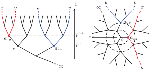
In the left figure, we already know that

	$$\displaystyle|x-y|_{p}=\mu(a_{xy})=|z(a_{xy})|_{p}=p^{-n-1}~,$$		(45)
	$$\displaystyle|u-v|_{p}=\mu(a_{uv})=\mu(c)=|z(c)|_{p}=p^{-n}~.$$		(46)

The right figure is another layout for the same graph. There is a radial coordinate $~z^{c}~$ of vertices depending on the distance between this vertex and the reference one $~c~$. For example, we can write

$$\displaystyle z^{c}(a_{xy})=p^{d(a_{xy},c)}=p^{1}~,~z^{c}(a_{uv})=p^{d(a_{uv},c)}=p^{2}~,~z^{c}(c)=p^{d(c,c)}=1~.$$

(47)

Each vertex(noted as $~a~$) in the right figure is a ball in $~\mathbb{Q}_{p}\cup\{\infty\}~$ containing boundary points which are on the “half-line” $~ca~$’s(half-lines which start from $~c~$, pass through $~a~$ and go to the boundary). The reference vertex $~c~$ contains all the boundary points, namely $~c=\mathbb{Q}_{p}\cup\{\infty\}~$. Measure $\mu^{c}$ of vertices and distance $~|\cdot|_{p}^{c}~$ of boundary points can be introduced according to the right figure, which satisfy

	$$\displaystyle|x-y|_{p}^{c}=\mu^{c}(a_{xy})=|z^{c}(a_{xy})|_{p}=p^{-1}~,$$		(48)
	$$\displaystyle|u-v|_{p}^{c}=\mu^{c}(a_{uv})=|z^{c}(a_{uv})|_{p}=p^{-2}~.$$		(49)

They are different from $~\mu~$ and $~|\cdot|_{p}~$ in the left figure or which are used in this paper. For example, it can be found that

	$$\displaystyle\mu(a_{xy})<\mu(a_{uv})~,~\mu^{c}(a_{xy})>\mu^{c}(a_{uv})~,$$		(50)
	$$\displaystyle|x-y|_{p}<|u-v|_{p}~,~|x-y|_{p}^{c}>|u-v|_{p}^{c}~.$$		(51)

$~\mu^{c}~$ and $~|\cdot|_{p}^{c}~$ are the measure and distance used in [9].

Consider the equation

$$\displaystyle Z_{M}[J]=\frac{\int_{\textrm{T}_{p}}\mathcal{D}\phi e^{-S+\sum_{a\in E_{M}}\phi_{a}J_{a}}}{\int_{\textrm{T}_{p}}\mathcal{D}\phi e^{-S}}=\frac{\int_{E_{M}}\mathcal{D}\phi\int_{\textrm{T}_{p}\setminus E_{M}}\mathcal{D}\phi e^{-S+\sum_{a\in E_{M}}\phi_{a}J_{a}}}{\int_{E_{M}}\mathcal{D}\phi\int_{\textrm{T}_{p}\setminus E_{M}}\mathcal{D}\phi e^{-S}}=\frac{\int_{E_{M}}\mathcal{D}\Phi e^{-S_{M}+\sum_{a\in E_{M}}\Phi_{a}J_{a}}}{\int_{E_{M}}\mathcal{D}\Phi e^{-S_{M}}}~.$$

(52)

Ignoring denominators and setting $~J=0~$, we can write

$$\displaystyle\int_{\textrm{T}_{p}\setminus E_{M}}\mathcal{D}\phi e^{-S}\sim e^{-S_{M}}\xrightarrow{M\to\infty}\int_{\textrm{T}_{p}}\mathcal{D}\phi e^{-S}\sim e^{-S_{M\to\infty}}~.$$

(53)

Therefore, $~S_{M}~$($~S_{M\to\infty}~$) can be regarded as the effective action after integrating out fields on $~\textrm{T}_{p}\setminus E_{M}~$($~\textrm{T}_{p}~$). Now let’s identify $~\textrm{T}_{p}~$ as a $~p$-adic version of AdS spacetime [22]. According to the spirit of AdS/CFT:

$$\displaystyle\langle e^{\int dxO\phi_{0}}\rangle_{\textrm{CFT}}=\int_{\textrm{AdS}}\mathcal{D}\phi e^{-S}\Big|_{\phi_{\partial\textrm{AdS}}=\phi_{0}}~,$$

(54)

where $~\partial\textrm{AdS}~$ is the boundary of AdS and the fluctuation of gravity has been ignored, $~e^{-S_{M\to\infty}}~$ should be directly proportional to the generating functional of some CFT over $~\mathbb{Q}_{p}~$, whose two-point function reads

$$\displaystyle\frac{\delta^{2}e^{-S_{M\to\infty}}}{\delta\Phi_{x}\delta\Phi_{y\neq x}}\Big|_{\Phi=0}=\frac{p(p-1)}{(p+1)L^{2}}\frac{1}{|x-y|_{p}^{2}}~.$$

(55)

It is consistent with [22] if setting $~\eta_{p}=1~,~\Delta=n=1~$ there and $~L=1~$ in (55). On the other hand, if not taking the limit $~M\to\infty~$, the following calculation should give a two-point function of some deformed CFT over (coarse-grained) $~\mathbb{Q}_{p}~$:

$$\displaystyle\frac{\delta^{2}e^{-S_{M}}}{\delta\Phi_{a}\delta\Phi_{b\neq a}}\Big|_{\Phi=0}=\frac{(p-1)^{2}}{L^{2}}A_{\frac{d(a,b)}{2}}=\frac{(p-1)^{2}}{L^{2}}\sum_{n=\frac{d(a,b)}{2}}^{\infty}\frac{1}{(p^{n}-1)(p^{n+1}-1)}~,$$

(56)

where $~d(a,b)=2,4,6,8,\cdots~$ is a positive even number and $~E_{M}=\{a,b,\cdots\}~$ is a coarse-grained $~\mathbb{Q}_{p}~$. Remember that each element in $~E_{M}~$ is a ball in $~\mathbb{Q}_{p}~$. (56) can be regarded as a counterpart to the two-point function of a deformed CFT living on the cutoff boundary of AdS over $~\mathbb{R}~$.

In this paper, we manage to reconstruct fields in the bulk from those on the finite boundary of $~\textrm{T}_{p}~$ (27). Then with the help of calculating techniques in [9], the effective field theory is calculated by integrating out fields on the entire $~\textrm{T}_{p}~$ except those on the finite boundary (39). According to the spirit of AdS/CFT, two-point functions of dual theories are read out: (55) on the infinite boundary and (56) on the finite boundary. The former is a two-point function of a CFT over $~\mathbb{Q}_{p}~$ which is consistent with [22], and the latter is a two-point function of a deformed CFT which should be compared with that in AdS/CFT over $~\mathbb{R}~$ with a cutoff AdS boundary.

Some problems still need to be explored. For example, i)relations between field spaces discussed in section 2 and those in [13, 30] are still unclear. Different field spaces or boundary conditions sometimes lead to different results; ii)it may be a hard problem to find out what “deformed CFT” is which gives a two-point function like (56). It is known that the counterpart over $~\mathbb{R}~$ can be regarded as a $~T\bar{T}$-deformed CFT [36]; iii)the same calculation on $~p\textrm{AdS}~$ is interesting. $p\textrm{AdS}~$ [22, 25] is another $~p$-adic version of AdS spacetime whose finite boundary is exactly $~\mathbb{Q}_{p}~$ but not the coarse-grained one.

This work is supported by NSFC grant no. 11875082.

References

- [1] I. V. Volovich. NUMBER THEORY AS THE ULTIMATE PHYSICAL THEORY. CERN-TH-4781/87, 1987.
- [2] V. S. Vladimirov. Generalized functions over the field of -adic numbers. Russian Mathematical Surveys, 43:19-64, 1988. doi:10.1070/RM1988v043n05ABEH001924.
- [3] L. Brekke and P. G. O. Freund. -adic numbers in physics. Phys. Rept., 233:1-66, 1993. doi:10.1016/0370-1573(93)90043-D.
- [4] V. S. Vladimirov, I. V. Volovich and E. I. Zelenov. -adic analysis and mathematical physics. Ser. Sov. East Eur. Math., 1:1-319, 1994.
- [5] I. V. Volovich. -ADIC STRING. Class. Quant. Grav., 4:L83, 1987. doi:10.1088/0264-9381/4/4/003.
- [6] V. S. Varadarajan. Arithmetic Quantum Physics: Why, What, and Whither. Proc. Steklov Inst. Math., 245:258-265, 2004.
- [7] P. G. O. Freund and M. Olson. NONARCHIMEDEAN STRINGS. Phys. Lett. B, 199:186-190, 1987. doi:10.1016/0370-2693(87)91356-6.
- [8] P. G. O. Freund and E. Witten. ADELIC STRING AMPLITUDES. Phys. Lett. B, 199:191, 1987. doi:10.1016/0370-2693(87)91357-8.
- [9] A. V. Zabrodin. Nonarchimedean Strings and Bruhat-tits Trees. Commun. Math. Phys., 123:463, 1989. doi:10.1007/BF01238811.
- [10] M. Heydeman, M. Marcolli, I. Saberi, and B. Stoica. Tensor networks, -adic fields, and algebraic curves: arithmetic and the AdS3/CFT2 correspondence. Adv. Theor. Math. Phys., 22:93-176, 2018. doi:10.4310/ATMP.2018.v22.n1.a4.
- [11] S. S. Gubser, M. Heydeman, C. Jepsen, M. Marcolli, S. Parikh, I. Saberi, B. Stoica and B. Trundy. Edge length dynamics on graphs with applications to -adic AdS/CFT. JHEP, 06:157, 2017. doi:10.1007/JHEP06(2017)157.
- [12] S. S. Gubser, C. Jepsen, and B. Trundy. Spin in -adic AdS/CFT. J. Phys. A, 52:144004, 2019. doi:10.1088/1751-8121/ab0757.
- [13] A. Huang, B. Stoica, and S. T. Yau. General relativity from -adic strings. BRX-TH-6643, Brown HET-1778. arXiv: 1901.02013.
- [14] A. Huang, B. Stoica, X. Xia and X. Zhong. Bounds on the Ricci curvature and solutions to the Einstein equations for weighted graphs. nuhep-th/20-04. arXiv: 2006.06716.
- [15] S. Ebert, H. Y. Sun and M. Y. Zhang. Probing holography in -adic CFT. arXiv: 1911.06313.
- [16] A. Bhattacharyya, L. Y. Hung, Y. Lei and W. Li. Tensor network and (-adic) AdS/CFT. JHEP, 01:139, 2018. doi:10.1007/JHEP01(2018)139.
- [17] L. Y. Hung, W. Li and C. M. Melby-Thompson. -adic CFT is a holographic tensor network. JHEP, 04:170, 2019. doi:10.1007/JHEP04(2019)170.
- [18] M. Heydeman, M. Marcolli, S. Parikh and I. Saberi. Nonarchimedean Holographic Entropy from Networks of Perfect Tensors. CALT-TH-2018-053. arXiv: 1812.04057.
- [19] J. M. Maldacena. The Large N limit of superconformal field theories and supergravity. Int. J. Theor. Phys., 38:1113-1133, 1999. doi:10.1023/A:1026654312961.
- [20] S. S. Gubser, I. R. Klebanov and A. M. Polyakov. Gauge theory correlators from noncritical string theory. Phys. Lett. B, 428:105-114, 1998. doi:10.1016/S0370-2693(98)00377-3.
- [21] E. Witten. Anti-de Sitter space and holography. Adv. Theor. Math. Phys., 2:253-291, 1998. doi:10.4310/ATMP.1998.v2.n2.a2.
- [22] S. S. Gubser, J. Knaute, S. Parikh, A. Samberg and P. Witaszczyk. -adic AdS/CFT. Commun. Math. Phys., 352:1019-1059, 2017. doi:10.1007/s00220-016-2813-6.
- [23] S. S. Gubser and S. Parikh. Geodesic bulk diagrams on the Bruhat-Tits tree. Phys. Rev. D, 96:066024, 2017. doi:10.1103/PhysRevD.96.066024.
- [24] P. Dutta, D. Ghoshal and A. Lala. Notes on exchange interactions in holographic -adic CFT. Phys. Lett. B, 773:283-289, 2017. doi:10.1016/j.physletb.2017.08.042.
- [25] F. Qu and Y. h. Gao. Scalar fields on AdS. Phys. Lett. B, 786:165-170, 2018. doi:10.1016/j.physletb.2018.09.043.
- [26] M. Marcolli. Holographic codes on Bruhat-Tits buildings and Drinfeld symmetric spaces. Pure Appl. Math. Quart., 16:1-33, 2020. doi:10.4310/PAMQ.2020.v16.n1.a1.
- [27] C. B. Jepsen and S. Parikh. -adic Mellin Amplitudes. JHEP, 04:101, 2019. doi:10.1007/JHEP04(2019)101.
- [28] L. Y. Hung, W. Li and C. M. Melby-Thompson. Wilson line networks in -adic AdS/CFT. JHEP, 05:118, 2019. doi:10.1007/JHEP05(2019)118.
- [29] C. B. Jepsen and S. Parikh. Recursion Relations in -adic Mellin Space. J. Phys. A, 52:285401, 2019. doi:10.1088/1751-8121/ab227b.
- [30] F. Qu and Y. h. Gao. The boundary theory of a spinor field theory on the Bruhat-Tits tree. Phys. Lett. B, 803:135331, 2020. doi:10.1016/j.physletb.2020.135331.
- [31] L. Chen, X. Liu and L. Y. Hung. Bending the Bruhat-Tits Tree I:Tensor Network and Emergent Einstein Equations. arXiv: 2102.12023.
- [32] L. Chen, X. Liu and L. Y. Hung. Bending the Bruhat-Tits Tree II: the -adic BTZ Black hole and Local Diffeomorephism on the Bruhat-Tits Tree. arXiv: 2102.12024.
- [33] L. Chen, X. Liu and L. Y. Hung. Emergent Einstein Equation in -adic CFT Tensor Networks. arXiv: 2102.12022.
- [34] V. Balasubramanian and P. Kraus. Spacetime and the Holographic Renormalization Group. Phys. Rev. Lett., 83:3605–3608, 1999. doi:10.1103/physrevlett.83.3605.
- [35] J. de Boer, E. P. Verlinde and H. L. Verlinde. On the holographic renormalization group. JHEP, 08:003, 2000. doi:10.1088/1126-6708/2000/08/003.
- [36] L. McGough, M. Mezei and H. Verlinde. Moving the CFT into the bulk with . JHEP, 04:010, 2018. doi:10.1007/JHEP04(2018)010.
- [37] G. Giribet. -deformations, AdS/CFT and correlation functions. JHEP, 02:114, 2018. doi:10.1007/JHEP02(2018)114.
- [38] P. Kraus, J. Liu and D. Marolf. Cutoff AdS3 versus the deformation. JHEP, 07:027, 2018. doi:10.1007/JHEP07(2018)027.