An RL-Based Adaptive Detection Strategy to Secure Cyber-Physical Systems
Abstract
Increased dependence on networked, software based control has escalated the vulnerabilities of Cyber Physical Systems (CPSs). Detection and monitoring components developed leveraging dynamical systems theory are often employed as lightweight security measures for protecting such safety critical CPSs against false data injection attacks. However, existing approaches do not correlate attack scenarios with parameters of detection systems. In the present work, we propose a Reinforcement Learning (RL) based framework which adaptively sets the parameters of such detectors based on experience learned from attack scenarios, maximizing detection rate and minimizing false alarms in the process while attempting performance preserving control actions.
Index Terms:
Cyber-physical systems, security, adaptive threshold, reinforcement learning, formal methodsI Introduction
While security is of paramount importance in CPS [1], the real time hard deadlines of the safety critical functions and availability of limited computing resources constitute the major constraints to secure CPS design. Traditional heavy-weight cryptographic encryption techniques (like RSA, AES) along with MACs cannot be used in most of the cases as they lead to both computation and communication overhead [2]. One alternative is to design light-weight attack detectors by exploiting control-theoretic properties. Such detectors leverage the features of various state-observers like Luenberger or Kalman filter that the controller unit of almost every CPS comes with. These observers estimate the state of the plant by computing residue as the difference between actual and observed sensor data. The detector compares this residue with a predefined threshold to identify an anomaly [3]. Though observers can be useful in monitoring the system’s behavior, they cannot always be adjusted to detect unmodeled disturbances, like faults and attacks. Reducing observer gain may render it insensitive towards small changes in system states, while increased observer gain will lead to increased estimation error covariance, which in turn will degrade the system’s control performance. To overcome this limitation, the statistical change detection methods, like -test, Cumulative Sum (CUSUM) [4, 5], etc. are applied on the residue, before it is compared to the threshold. However, the constant threshold used by these residue based detectors may increase the false alarm rates (FAR) by misinterpreting measurement noise as attack, leading to unnecessary degradation in control performance. Moreover, recent research [6, 7] have shown how a stealthy attacker can fool such detectors by crafting perturbation sequences which create residues that are small enough (i.e. below threshold) to be classified as noise. Therefore, the fundamental question that arises is, whether the detection threshold for such monitors in CPS implementations can be dynamically adjusted based on the deployment environment so that FAR is minimized while even small attack efforts can be detected. In the present work we propose an intelligent detection scheme that strives to achieve this goal.
Some recent research efforts, for example [7, 8, 9], have addressed this problem of balancing between FAR and detectability in the CPS context. However, they have the following limitations that we have addressed in the current work. Unlike [8], the proposed detector focuses on identifying attacks on CPS rather than faults. In [8], the authors have formulated a non-linear programming problem to synthesize adaptive thresholds, considering operating regions. When the system is online, a threshold is selected from the pre-calculated ones to detect transient faults, based on which operating region the system is currently working in. In case of attack, things are more difficult as an attacker can be smart enough to modify its action to remain stealthy. In [7], the authors have presented two greedy algorithms based on formal methods to synthesize monotonically decreasing variable threshold based detectors to thwart targeted performance degrading attacks while minimizing FAR. However, they have defined the CPS system requirement in terms of settling time. In such works it is often straightforward to design attack vectors through constraint solving such that the settling time property is satisfied while some other safety property gets violated causing critical damage to the system. On the contrary, our approach interprets system safety in terms of a safe operating region. Considering that an attacker may force the system to migrate beyond this safety boundary at any time instant, our proposed detector would try to detect such attack efforts as early as possible.
CPSs are usually designed as closed loop feedback systems with both controller and observer in place, both working together to ensure stability while minimizing the effect of noise. Aim of an attacker would be to remain stealthy and destabilize the closed loop dynamics by failing the efficacy of the controller and the estimator. Therefore, while designing a detector we must also consider such an attack model. Moreover, in the view of real time constraint of the safety critical CPSs, the adaptive threshold generation process must be efficient in terms of timing overhead. Though, the authors of [9] have drawn similar motivation like ours and presented an attacker-defender game to solve the adaptive threshold selection problem, their work lacks these considerations.
Another important aspect while designing an intelligent secure CPS is the mitigation of an attack’s effect, i.e. when an attacker is detected by the detector system and the system is still within the safety boundary, how can its effect be mitigated at the earliest ? The approach in [10] proposes a Reinforcement Learning (RL) based robust control strategy for autonomous vehicle (AV) control in the presence of an attacker who modifies the spacing information between vehicles. The method leverages the fact that measurement information (velocity of other vehicles) is drawn from multiple sensors and learns the optimal weights of these sensors that mitigate the attack’s effect. However, this work is applicable to a specific CPS and also the authors do not consider any active security primitive like detection systems. In [11], the authors formulate a secure state estimation problem followed by RL based optimal controller design to void the effects of detected attacks. Though the approach is based on a general CPS model, they have used a constant threshold based attack detector which may suffer from high FAR. In general, the fact that a well-trained RL agent is realizable for safety critical CPSs with real time requirements has already been established in other contexts like energy efficiency[12].
In this work, we consider that the communication channel between the plant and controller is vulnerable, i.e. an attacker can gain access to the network and add spurious data to every communication between plant and controller. Such an attack is called false data injection (FDI) attack. Assuming that the attacker has complete knowledge of the system and associated detector, it can intelligently craft an attack to induce maximum damage to the system while remaining stealthy.

We present an intelligent secure CPS model that consists of: an adaptive attack monitor that thwarts an FDI attack, and a robust controller that mitigates the effect of such attacks. Considering an attack as unmodeled disturbance that does not follow any defined distribution; we propose an RL based baseline framework as shown in Fig. 1 that leverages the following RL agents.
- 1.
We present a novel detector for CPS attacks which leverages RL based adaptive threshold selection (Fig. 1). The choice of the threshold is based on minimization of FAR while keeping it below a predefined upper bound.
- 2.
We present an RL based robust control strategy (Fig. 1) that would strive for preserving control performance in the presence of FDI attacks. When no attack takes place, the system operates with an optimal controller that ensures high performance by restricting the trajectory inside a preferable operating region. When an attack effort is detected with the system still within its safety boundary, the proposed robust controller brings the system back to its preferable operating region.
- 3.
For the RL based detector and controller to learn from experience, one needs to provide FDI attack vectors that are both stealthy and able to steer the system away from safe operations. Our third RL agent mimics such attack behavior in the training phase of the system.
- 4.
We establish the usefulness of our multi-agent secure CPS model by considering attack scenarios for well known CPS benchmarks and achieving significant performance improvement w.r.t. baseline.
II Secure CPS Model
In the absence of an adversary, the closed loop dynamics of a CPS can be presented as a discrete linear time-invariant (LTI) system,
| (1) |
where, is the system state vector, is the measurement vector obtained from available sensors at -th time stamp; are the system matrices. We consider that the initial state , the process noise and the measurement noise are independent Gaussian random variables. Further, in every -th sampling instant, the observable system state is estimated using system output while minimizing the effect of noise, and used for computing the control input . The symbol denotes the residue i.e. the difference between the measured and the estimated outputs. The observer gain and controller gain ensures that both and are stable. The system has a detector unit (Fig. 1) which computes a function and compares it with a threshold to identify any anomalous behavior of the system. Considering an FDI attack, where the attacker injects false data and (Fig. 1) to the sensor data and control signal respectively, the equation of the system dynamics will become,
| (2) |
Here, , , , , , represent plant state, estimated plant state, forged sensor data, residue, control signal, and forged control signal respectively in an attack scenario. In the present work we consider as the popular -test commonly employed in existing works on secure CPS [3].
-Test and -Distribution : The -test is one of the most widely used statistical tests for examining the independence of two or more categorical variables. Given the observed count and the expected count of each category , statistics can be computed as . Here, is the number of categories. Smaller value of signifies more correlation between the categories. Now, consider random variables that follow standard Gaussian distribution. Sum of the squares of these random variables follow a distribution of degrees of freedom (dof) defined as, . Here, denotes the Gamma function and mean of this distribution is . Given the -distribution of dof and the statistics, we can decide whether to accept or reject a specified null hypothesis. For example, a null hypothesis can be whether a random Gaussian vector has the expected mean and variance. Therefore, -test can be used to detect anomalies in dynamical systems [13], like CPSs[3]. -Test on an dimensional random variable gives . follows a -distribution with dof = . With respect to a given threshold , we say an anomaly is detected if at some time stamp .
III Proposed Methodology
In this section, we elaborately discuss the three principal components of our proposed adaptive secure CPS model: i) an adaptive threshold synthesis method, ii) an intelligent attack generation method, and iii) a robust control strategy. Finally, we present a multi-agent RL framework that binds the above three components to ensure intelligent attack detection and mitigation.
III-A Optimal Threshold Synthesis
We present a residue based attack detection system where we consider the Kalman filter as the estimator. The proposed detector will adaptively select a threshold at every -th sample. Let, for the discrete LTI system shown earlier, the estimation error be defined as . The Gaussian assumptions of noise and initial states ensure that follows a normal distribution with mean. We denote the steady state covariance matrix of this estimation error with . So the system residue , calculated in the Kalman estimator can be expressed as (see Eq. 1). Given that both estimation error and measurement noise are Gaussian distributed with zero mean and are independent of each other, the residue is normally distributed with mean and covariance matrix given .
We use -test on to find out how much the distribution of actual plant state and its estimate vary from each other. Let denote the -test result at -th sample and . Here, is the window size of -test. In this case, the degree of freedom is , where is the number of available sensors in the plant. In a normal scenario (no attack), follows distribution with mean (Fig. 2). Let be the threshold that is currently (at -th sampling instance) being used by our variable threshold based detector unit. Then, ’s probability density function (PDF) along with its cumulative distribution function with respect to can be defined as, . Here, and are ordinary and lower incomplete gamma functions respectively. We say it is a false alarm when even in the absence of an attacker.
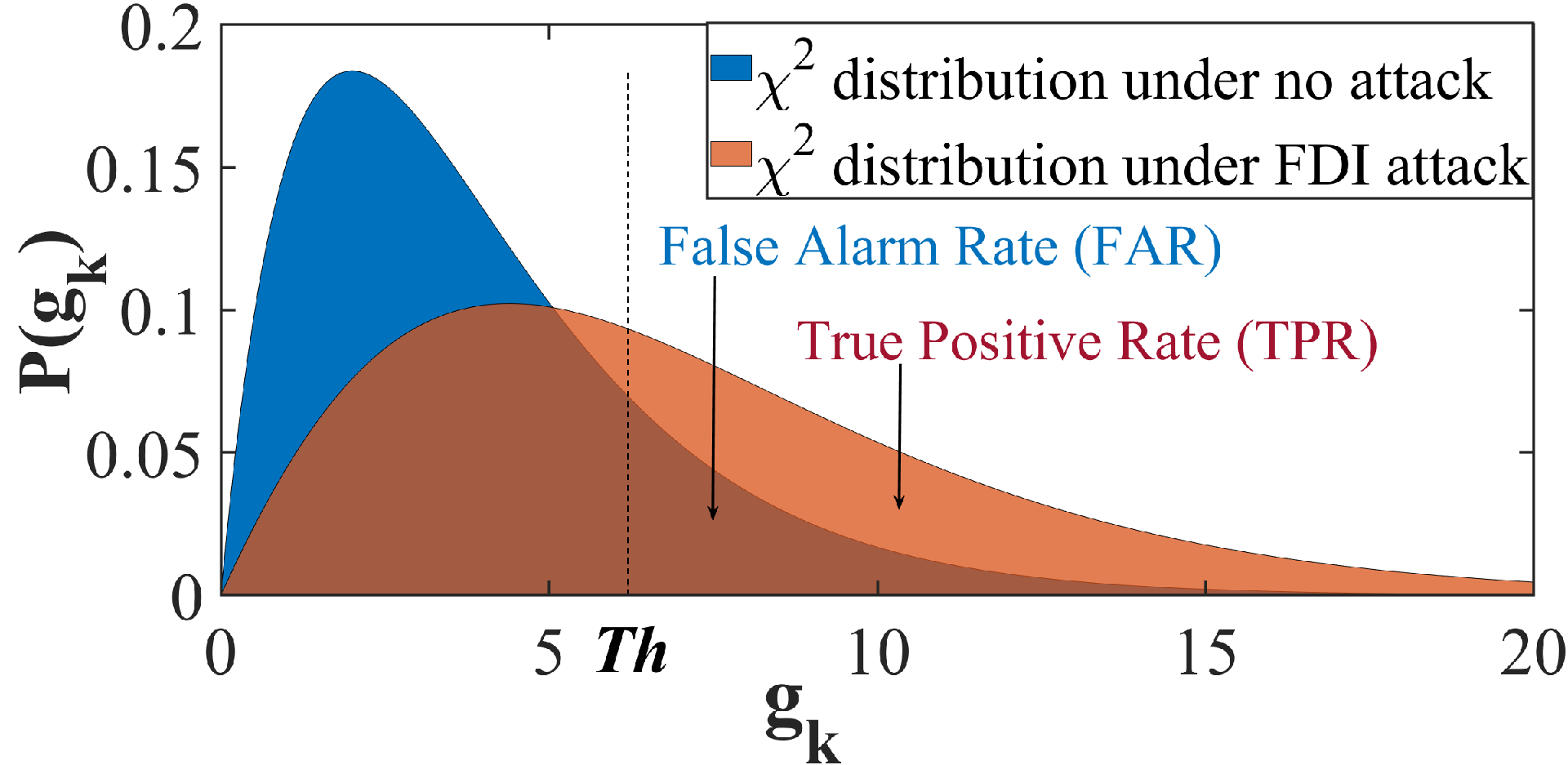
So false alarm rate (FAR) is the ratio of the number of times when the alarm has been raised falsely and the total number of alarms raised. In Fig. 2, the blue curve and the maroon curve represent the distribution of under no attack and attack respectively. Therefore, FAR should be the fraction of area under the probability distribution curve of un-attacked that is contained by the part beyond and computed as .
Now, in presence of an FDI attack, where spurious data and are added to the sensor and the actuator data respectively, this leads to non-centrality of the -test (the maroon curve in Fig. 2) result obtained for the residue under attack as established next.
Theorem 1
Considering an FDI attack on an LTI system as specified in Eq. 2, the -test on residue follows a non-central -distribution.
Proof: Under FDI attack, the estimation error at -th sample is given by . Let be the difference between the estimation error under attack and no attack scenarios. Thus, . Considering that the mean of the estimation error is and measurement noise is independent of the estimation error and sensor attack, the covariance of the residue generated due to an FDI attack can be computed as where,
Here, the notations and denote the mean and variance respectively of any variable , and denotes the covariance of for any . Using the expressions of and we get,
| (3) | ||||
Here, , . Since, by definition, covariance is positive semi definite and variance is positive, both , and consequently are positive definite. Considering an FDI attack on the both control signal and sensor output, we apply -test on which gives . Therefore, the mean of the statistics of over an observation window of length can be computed as i.e.,
| (4) | ||||
The last inequality follows from the fact that is positive definite. Hence, the mean of is strictly greater than the mean of . This makes the distribution of a non-central one with non-centrality parameter .
Theorem 2
Leveraging the non-central distribution of statistics increases the detectability of a false data injection attack.
Proof: The non-central distribution of with mean and non-centrality parameter can be defined in terms of the following PDF[14], with denoting Bessel function. With respect to , we say an FDI attack is detected if . This is a true positive case. Therefore, the true positive rate (TPR) of detecting an attack is computed as where . Essentially this is fraction of area under the distribution curve (Fig. 2) of beyond . Here, is Marcum Q-function [14]. In Theorem 1, we have proved that where is the mean of . This causes the non-central distribution of to be more shifted towards the right than the distribution of .
Moreover, the variance of is and variance of is , where . Clearly, . Therefore, the expected deviation of from is more than the expected deviation of from which makes the distribution of P() wider and thereby flatter (since the area under both curves is unity). Hence, the fraction of area under the curve beyond of P() is more than that in case of P() as shown in Fig. 2. So, the non-central distribution improves TPR i.e. attack detectability thus leading to for a properly chosen threshold parameter .
Given the dependence of on the parameters the problem of synthesizing an optimal detector can be formulated as following optimization problem:
aimed at minimizing and maximizing . Here are the constant weights of TPR and FAR respectively, is the maximum allowable FAR, and is maximum allowed sequence length. Given , the current sensor measurement vector, the solution of the above optimization problem is a pair , where and are the optimal window length and threshold respectively with respect to current measurement of the system states.
III-B Intelligent Attack Generation

Considering the discrete LTI system specified in Eq. 1, we classify the operating region of the system, as demonstrated in Fig. 3, in two primary subregions: i) safe region , and ii) preferable operating region where . The system becomes unsafe when it goes beyond the outermost region . The middle region defines the set of possible states in which system operation is preferred due to performance consideration. We formally define such preferable operating regions as robust invariance sets as follows.
Definition 1
By preferable operating region, we mean that starting from anywhere within , the controller ensures that the system will always remain within in the absence of any FDI attack. Note the choice of can be exercised depending upon system description and safety criteria. The invariant set based preferable operating region is chosen in practice as some -step invariant set within for which the controller guarantees satisfactory performance.
Synthesis of Preferable Operating Region : We present a Satisfiability Module Theory (SMT) aided constraint solving approach for computing for a given safety-critical CPS in Algo. 1. The getPerformanceRegion( ) function takes as input the system matrices , controller gain , observer gain , safety region , and the forward step count for an -step invariant set. The preferable operating region is defined as a fraction of i.e. , . For an dimensional system with representing any real interval. Initially, we consider where and compute accordingly in line 4. Then, the plant state is initiated symbolically from (lines 4-5). We unroll the state progression times following Eq. 1 in lines 9-11. For to be the desired preferable region, after steps, plant state must reside within i.e., . This symbolic constraint is provided as an assertion (line 12). Negation of this assertion, i.e. , is passed to the SMT solver Z3 [15]. Z3 tries to find a value of for which can be satisfied. If such an assignment of is found, it implies that there exists an initial state of the system the current candidate , starting from which the system does not converge back to in steps. Note that we consider the reference point of the system is . The optimal LQG controller with gain guarantees to keep the system close to the reference point at steady state. Therefore, the algorithm retries by increasing by a step and looks for a larger (line 13-14). Otherwise, current is returned as final (line 15).
We set as in our experiments. Thus, it is formally guaranteed that the system will always remain within when no attack is taking place provided it has been initiated from itself. In this work, we design as a Linear-Quadratic-Gaussian (LQG) controller. In general, any optimal control framework is applicable though.
In the CPS context, the attacker’s motive is to steer the system beyond the safe set while trying to remain stealthy by reducing the TPR. Given the sensor measurement , we present this attack estimation problem as the following optimization problem:
Here, and are the same weights used in for the optimal threshold cost function . Since the attack generation method will be used for experience learning of threshold tuner and robust control RL agents, it is imperative that assumes knowledge about and tries to negate its cost objective. This is captured in the first two component terms of . The last component of accounts for deviation of the current system state from the safety boundary using a quadratic weighted distance metric where is a diagonal matrix consisting of relative weights corresponding to criticality of each dimension. Also, indicate the allowable sensor range, and actuation saturation range respectively. The solution of the above optimization problem is a possible attack vector that can breach the safety barrier while being stealthy, i.e. by nullifying the detector objective function . In both implicit constraints are system and detector dynamics.
III-C Robust Controller Design
The LQR controller gain is designed to provide optimal control action with respect to control cost under no attack scenario. However, it may not guarantee robustness against FDI attacks. To mitigate effect of an FDI attack, we propose a robust control strategy that will be triggered only when the adaptive threshold based detector (Sec. III-A) detects an FDI attack and the system at the moment of attack detection. Given the forged sensor data , we compute such a robust control action by solving the following optimization problem:
Naturally, system dynamics is an implicit constraint here. We have used the same weight matrix from to nullify the attack’s effect (assuming the knowledge of the attack generation module about all other cost functions). The solution of the above optimization problem is a control input that minimizes the damage induced by the attacker by bringing the system back inside (thereby, inside ). Note that is not optimal w.r.t. performance unlike an optimal controller; being robust it prioritizes safety. Thus, we are allowing higher control effort as long as it does not exceed the actuation saturation limit as the objective of this controller would be bringing the system back to in minimum time. Once inside , the system switches to the optimal controller.

III-D The Reinforcement Learning Framework
Since an attacker may exhibit unknown dynamics, the central idea of the work is to learn an adaptive attack detection scheme along with a robust controller for attack mitigation whenever possible. Due to scarcity of system specific labeled false data and the requirement of learning parameters in dense domains, we employ the popular Deep Deterministic Policy Gradient (DDPG) algorithm [16] which outputs deterministic actions instead of optimized action distribution over the continuous action space. The overall RL framework is shown in Fig. 4. A Deep Q-Network to criticize and update the actor policy by calculating the Q value against the state and chosen action.
We first describe the environment and agent specifications to understand the learning process that helps derive the design parameters. Since a plant-controller closed loop system, equipped with a -based detector, as shown in Fig. 1) is the system under test here, we design our environment by modeling such a closed loop system. Our methodology uses three DDPG agents () that interact with this environment. By observing certain parameters from the environment (), the agents learn how to intelligently choose an action () to influence it as they want. The following table lists the observation and action variables.
| RL Agent | Observations | Actions |
|---|---|---|
| Attacker Agent | ||
| Detector Agent | ||
| Controller Agent |
The Attacker Agent () is designed to intelligently inject false data into the system. We design a reward function for , that is built with the components of . The FDI attacker agent tries to solve the optimization problem in every sampling iteration during training, by exploiting several actions while exploring the action space. These transitions are then stored as experiences. The training algorithm learns the highest expected return from the experiences and updates the RL policy to earn it. This helps it eventually choose the optimal action i.e. the optimal false data to inject into the sensors and actuators , that generates the maximum value of as the reward for the FDI attacker agent. Similarly for Threshold-based Detector Agent (), a reward function is designed with the components of . The agent intelligently chooses the optimal change detection parameters like threshold and detection window length by optimizing the objective function i.e. aiming the maximum reward . The reward function is also designed with for to choose an optimal control input that generates the maximum reward. The Attack mitigating Controller Agent () is activated when an attack is detected in the considered closed loop system (refer Algo. 2).


Given a secure CPS model, we train these model-free DDPG agents so that they act according to their designated roles in the environment, which is a simulated secure CPS model. Using standard DDPG training algorithm, how these agents () learn to interact with our multi-agent RL environment collaboratively and competitively, is depicted in Fig. 4. For example, from the reward and objective functions we can see that the detector agent always tries to win against the attacker agent by competitively choosing an action(-detection threshold and observation window) to detect its (’s) actions (FDIs). Once the attack is detected, the controller agent then tries to nullify the effects of these actions (attacks/FDIs output by the attacker ) by choosing an optimal action (attack mitigating control input) from the training experiences. The attacker agent also tries to contest these two agents by optimally launching a hard-to-detect yet successful FDI in every iteration. In a way, is collaborating with and to help them learn the system characteristics under FDI attack. Algo. 2 represents the overall methodology.
IV Results
Systems and Framework Specifications: Automotive systems have heterogeneous communication protocols for internal communications between the Electronic Control Units (ECUs) that execute real time control tasks. Vulnerability in any of those protocols (eg. Controller Area Network) can grant an easy access to the attacker to manipulate majority of the system communications. This motivates us to apply our RL based monitoring framework to one such automotive CPS, namely Trajectory Tracking Controller (TTC). TTC regulates the deviation of a vehicle from a given trajectory () and a reference velocity () by applying proper acceleration [17]. Our RL based framework is built on MATLAB Reinforcement Learning Toolbox. As mentioned earlier we employ DDPG agents having a policy gradient based actor network coupled with a DQN based critic network. Both the actor and critic networks have 3 hidden layers with rectified liner activation units (ReLU) for better training considering the complexity of CPSs. We train this RL based monitoring framework with TTC for 3000 episodes with three RL agents. The system matrices (), sampling period (), controller and estimator gains () along with corresponding preferable operating region () and safety region () of the systems are given in Tab. II.
| Sys. | Specifications | |||||||||||
|---|---|---|---|---|---|---|---|---|---|---|---|---|
|
|
|
|
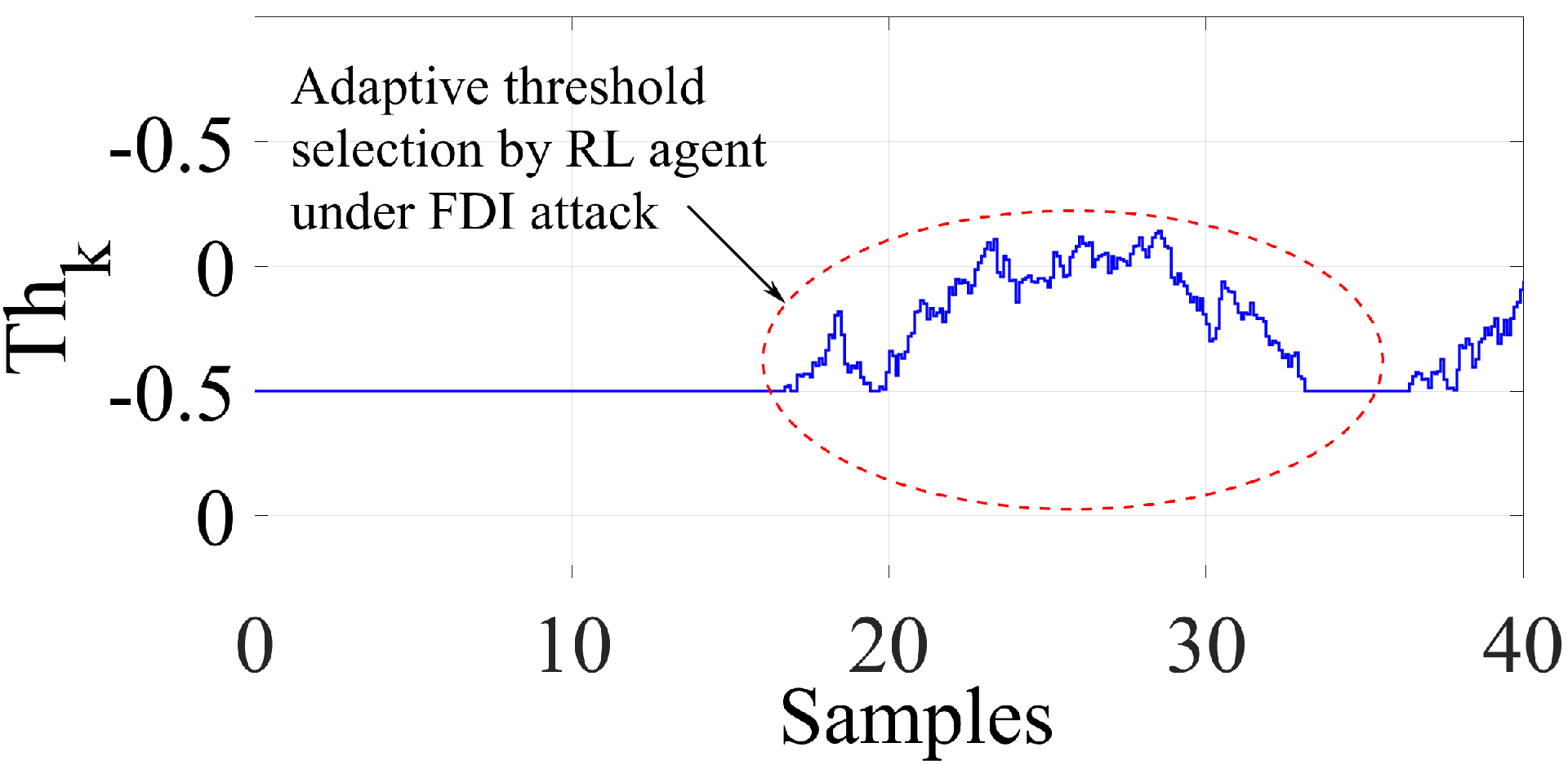
Experimental Results: As per our system specifications the TTC is equipped with a detector. To promise optimal resilience, while training, we assume the attacker is aware of the adaptive threshold based detector specifications (the currently chosen and ). We have trained the detector agent in the presence and absence of the attacker agent to reinforce the learning that differentiates an attacked and un-attacked situation. Given the safety specifications of the system we first derive the preferable operating region of TTC using Algo .1. Intializing the system states from this region, we train the RL agents for 3000 episodes, each with 100 simulation instances in order to train them. As we can see in Fig. 5(b) , the detector agent explores and exploits different threshold values for different detection windows. This is an FDI attack scenario where the attacker agent injects optimal false data to make the system unsafe. For this, the -test value on the system residue changes as we see in Fig. 5(c). The detector agent starts by selecting for and changes the threshold to successfully detect most of the attack efforts. If we consider the maximum non-centrality induced by the optimal FDI attacker agent, TPR achieved by the adaptive detector agent is . Note that, as shown in Fig. 5(c) under the considered optimal attack scenario, the attacker is detected even before it is able to send the observed system state outside the preferable operating region (=7.5 for the output state, refer Tab. II). Hence the robust controller does not kick off and our adaptive detection system promises a cost effective control by early detection of attack.
In Fig. 5(a) as can be seen, our variable threshold based detector selects when there is no FDI attack in place. The average FAR achieved by the designed adaptive detection system during no attack situation is . As we can observe in Fig. 5(a), it manages to place the threshold above the -test values of system residues due to noises (under no FDI attack). Targeting the minimum FAR, consider a constant threshold based detector with is placed to detect FDI attacks. Then, it is clear from the statistics of residues under attack in Fig. 5(c) that many of the attack attempts would have remained undetected.
V Conclusion
The present work proposed a RL based secure CPS model and studied its usefulness through simulation using an automotive CPS benchmark. In future, we plan to create an automotive hardware-in-loop simulation infrastructure which will help us simulate automotive control loops and vehicle dynamics in a real time platform in order to check the timing performance of the proposed scheme in a more realistic setting.
References
- [1] A. Humayed, J. Lin, F. Li, and B. Luo, “Cyber-physical systems security—a survey,” IEEE Internet of Things Journal, vol. 4, no. 6, pp. 1802–1831, 2017.
- [2] A. Munir and F. Koushanfar, “Design and analysis of secure and dependable automotive cps: A steer-by-wire case study,” IEEE Transactions on Dependable and Secure Computing, 2018.
- [3] Y. Mo and B. Sinopoli, “False data injection attacks in cyber physical systems,” in SCS, Stockholm, 2010.
- [4] A. S. Willsky, J. J. Deyst, and B. S. Crawford, “Two self-test methods applied to an inertial system problem,” Journal of Spacecraft and Rockets, vol. 12, no. 7, pp. 434–437, 1975.
- [5] J. Giraldo, D. Urbina, A. Cardenas, J. Valente, M. Faisal, J. Ruths, N. O. Tippenhauer, H. Sandberg, and R. Candell, “A survey of physics-based attack detection in cyber-physical systems,” ACM Computing Surveys (CSUR), vol. 51, no. 4, pp. 1–36, 2018.
- [6] A. Teixeira et al., “Secure control systems: A quantitative risk management approach,” IEEE Control Systems Magazine, vol. 35, no. 1, pp. 24–45, 2015.
- [7] I. Koley, S. K. Ghosh, S. Dey, D. Mukhopadhyay, A. K. KN, S. K. Singh, L. Lokesh, J. N. Purakkal, and N. Sinha, “Formal synthesis of monitoring and detection systems for secure cps implementations,” in 2020 Design, Automation & Test in Europe Conference & Exhibition (DATE). IEEE, 2020, pp. 314–317.
- [8] Y. Baek and M. Jo, “Adaptive threshold generation for fault detection with high dependability for cyber-physical systems,” Appl. Sci., vol. 8, no. 11, 2018.
- [9] A. Ghafouri, W. Abbas, A. Laszka, Y. Vorobeychik, and X. Koutsoukos, “Optimal thresholds for anomaly-based intrusion detection in dynamical environments,” Lect. Notes Comput. Sci. (including Subser. Lect. Notes Artif. Intell. Lect. Notes Bioinformatics), vol. 9996 LNCS, pp. 415–434, 2016.
- [10] A. Ferdowsi, U. Challita, W. Saad, and N. B. Mandayam, “Robust deep reinforcement learning for security and safety in autonomous vehicle systems,” in 2018 21st International Conference on Intelligent Transportation Systems (ITSC). IEEE, 2018, pp. 307–312.
- [11] Y. Zhou, K. G. Vamvoudakis, W. M. Haddad, and Z.-P. Jiang, “A Secure Control Learning Framework for Cyber-Physical Systems under Sensor Attacks,” in 2019 Am. Control Conf. IEEE, jul 2019, pp. 4280–4285.
- [12] Y. Wang, C. Huang, and Q. Zhu, “Energy-efficient control adaptation with safety guarantees for learning-enabled cyber-physical systems,” arXiv preprint arXiv:2008.06162, 2020.
- [13] R. Da, “Failure detection of dynamical systems with the state chi-square test,” Journal of guidance, control, and dynamics, vol. 17, no. 2, pp. 271–277, 1994.
- [14] A. F. Siegel, “The noncentral chi-squared distribution with zero degrees of freedom and testing for uniformity,” Biometrika, vol. 66, no. 2, pp. 381–386, 1979.
- [15] L. De Moura et al., “Z3: An efficient smt solver,” in TACAS. Springer, 2008.
- [16] T. P. Lillicrap, J. J. Hunt, A. Pritzel, N. Heess, T. Erez, Y. Tassa, D. Silver, and D. Wierstra, “Continuous control with deep reinforcement learning,” 2019.
- [17] V. Lesi et al., “Integrating security in resource-constrained cyber-physical systems,” ACM TCPS, vol. 4, no. 3, pp. 1–27, 2020.