Patchworking the Log-critical locus of planar curvesThanks: The authors are grateful to Jens Forsgård and especially to Timur Sadykov and Dmitrii Bogdanov for providing the pictures based on the work [BKS16] that we used for Figure 5. A.R. acknowledges support from the Labex CEMPI (ANR-11-LABX-0007-01).
.
We establish a patchworking theorem à la Viro for the Log-critical locus of algebraic curves in . As an application, we prove the existence of projective curves of arbitrary degree with smooth connected Log-critical locus. To prove our patchworking theorem, we study the behaviour of Log-inflection points along families of curves defined by Viro polynomials. In particular, we prove a generalisation of a theorem of Mikhalkin and the second author on the tropical limit of Log-inflection points.
Key words and phrases:
Amoeba, contour, Log-critical locus, patchworking.2010 Mathematics Subject Classification
14H50, 14M24, 14T051. Introduction
A fundamental problem in real algebraic geometry is the topological classification of projective non-singular varieties of a fixed degree. For plane curves , the topological classification is known since the work of Harnack ([Har76]), but the ambient classification, that is the classification of topological pairs , is still open from degree .
A different but related classification problem is the one introduced in [Lan19]: for a given degree , classify the topological pairs where is a curve of degree and is the Log-critical locus. Recall that the Log-critical locus is the closure in of the critical locus of the map
Alternatively, the set is the critical locus of the restriction to of the moment map , where is the standard -simplex. Important related objects are the amoeba and its contour .
In analogy to the real locus of a real algebraic curve, the set is a smooth manifold of dimension 1, that is a disjoint union of ovals in the Riemann surface , provided that is generic. More precisely, the set of curves for which is singular is a semi-algebraic subset of real codimension in the set of all complex curves of degree , see [Lan19]. The complement to this discriminantal set turns out to be disconnected for , allowing distinct topological pairs for a given degree.
There exist strong connections between the ambient classification problem in real algebraic geometry and the classification of Log-critical loci. Indeed, it was observed by Mikhalkin in [Mik00] that for a real curve , the real part is a subset of . The inclusion taking place in gives valuable information on the inclusion . A striking example is given by the simple Harnack curves introduced in [Mik00]: if the inclusion is an equality, then the topological pair is uniquely determined by the degree. We also refer to [Lan15] for further results in this direction.
Up to now, not much is known on the classification of pairs for a given degree . As observed in [Mik00], the set is the pullback of under the logarithmic Gauss map . This implies that the number of connected components of satisfies
where is the degree of . There are very few general constructions of curves with prescribed values of . The first example comes from the simple Harnack curves of [Mik00]: for such curves, the set has connected components. In [Lan19], it was shown that can achieve all values between and . Besides the latter results, there is no general construction of pairs . In particular, there was no evidence up to now of the existence of a curve with smooth Log-critical locus satisfying .
Coming back to the classification of real algebraic curves, the most powerful tool to construct pairs is the Patchworking Theorem introduced by O. Viro, see [Vir84]. In its full generality, this theorem allows one to construct real algebraic hypersurfaces of a given degree in toric varieties by gluing a collection of hypersurfaces of smaller degrees using so-called Viro polynomials, see for instance the appendix of [GLS18] or [Ris93].
The main goal of the present paper is to prove an analogue of Viro’s Patchworking Theorem for Log-critical loci and study its applications to the associated classification problem. We obtain a patchworking theorem in the name of Theorem A that we use to construct curves whose Log-critical locus has a small number of connected components, see Theorem B. In particular, we show that for any degree , there exists a smooth curve such that is smooth and connected. In particular, we disprove Conjecture 1 in [Lan19].
The statement of Theorem A requires some technicalities and is therefore postponed to Section 3. In the meantime, let us illustrate the latter results with some examples. To begin with, let us consider the patchworking of the real algebraic curves and defined respectively by the polynomials
Here, we denote the Newton polygon of and the corresponding moment map, . The real part can be represented in 4 symmetric copies of , one copy per quadrant of . This representation, usually referred to as a chart of the curve, can be achieved by using an unfolding of that remember the signs of each quadrant, see Figure 1. Since the polynomials and agree with each other on the common edge , the Patchworking Theorem states that there exists a curve with Newton polygon and whose chart is isotopic to the gluing of the charts of and , see again Figure 1. Moreover, the curve can be defined as the zero set of the Viro polynomial
for small enough.
There is no direct generalisation of the charts of Figure 1 if we perturb the polynomials and in a complex direction since the real parts of and cease to exist. To fix this, we can first fold the 4 copies of each Newton polygon to a single one, considering the set instead of the chart of , see Figure 2. Secondly, we can trade the set for its superset , that is the contour of . We can use such kind of representations for an arbitrary patchwork. This provides an indirect picture on how the Log-critical loci of the various curves involved in the patchwork eventually glue together along the families of curves defined by the underlying Viro polynomial.
Instead of the polynomials , and used above, consider now
and the Viro polynomial
and add a tilde to every piece of notation. Then, Theorem A describe the set for a generic choice of the complex parameter , provided that is small. In Figure 3, we picture the patchworking procedure at the level of contour as well as the amoeba for the parameter . In the present case, Theorem A implies that , a fact that can be read from Figure 3. To our knowledge, this is the first instance of a curve whose Newton polygon is the 2-simplex and such that its critical locus is smooth and has exactly 2 connected components. An additional patchwork using the latter curve leads to a cubic curve whose Log-critical locus is smooth and connected. Concretely, if is the defining polynomial of , then the curve can be defined by the polynomial , see Firgure 4.
The efficiency of Theorem A for constructing curves with prescribed Log-critical locus relies on the variety of building blocks that are already at our disposal. In Section 5, we provide a collection of such building blocks that we use later on to prove Theorem B. Those blocks are curves in the Hirzebruch surface . If we denote the coordinates of , these curves intersect the divisor exactly once. More importantly, they have the remarkable property that each intersection point with the divisor is contained in a single component of the Log-critical locus. The latter phenomenon can be observed in Figure 5 where the contour of such curves is depicted. There, we can observe the “birth” of each of the tentacles going upwards, involving exactly one component of the Log-critical locus.
To obtain Theorem A, we study the behaviour of Log-inflection points along families of curves defined by Viro polynomials. Recall that a Log-inflection point is a ramification point for the the Logarithmic Gauss map . The relative position with of the corresponding branching points in governs the topology of the pair since . While patchworking a collection of curves , the 1-parameter family of curves defined by the underlying Viro polynomial can be compactified with the reducible curve at , using an appropriate toric -fold. When tends to , some of the Log-inflection points of the generic curve concentrate at the nodal points of the central curve . We describe the asymptotic of these points in Theorem D, see Section 4. The latter result is the cornerstone of the proof of Theorem A. It also leads to a generalisation of a theorem of Mikhalkin and the second author (see [MR18]) in the name of Theorem C. The latter theorem describes the tropical limit of the Log-inflection points along families of curves defined by generic Viro polynomials. The original statement [MR18, Theorem 3] asserts that Log-inflection points accumulate by pairs at the midpoint of every bounded edge of a tropical curve, if the tropical curve is non-singular. We prove that the same phenomenon occurs for families of curves defined by generic Viro polynomials associated to arbitrary subdivisions. In particular, the limiting tropical curve may be singular in this context. Eventually, we show in the appendix that the genericity assumption on the Viro polynomial is necessary. To do so, we exhibit Viro polynomials for which the tropical limit of some Log-inflection points is located at 1/3 of a bounded edge of the tropical limit.
2. Setting
2.1. Viro polynomial
Throughout this text, the symbol refers to a lattice polygon, that is the convex hull in of a finite set of points in . We denote by the Newton polyhedron of any Laurent polynomial . We denote by the polarized toric surface associated to , see [GKZ08, Chapter 5]. The monomial embedding (1.2) of the latter reference allows to identify the space of section with the projectivisation of the space of Laurent polynomials whose Newton polygon is contained in . The toric surface provides a compactification of with a chain of toric divisors. Each such divisor is isomorphic to and correspond to an edge of via the moment map.
Definition 2.1.
A subdivision of a lattice polygon is a set of lattice polygons such that:
- •
,
- •
if , then the intersection is a common face to and .
A subdivision of is said to be convex if there exists a convex piecewise-linear function whose domains of linearity coincide with the polygons . If such a function exists, then it can be taken in such a way that . We call such a function -convex.
For any -convex function and any Laurent polynomial
we define the associated Viro polynomial to be the Laurent polynomial
For any , we denote by the truncation of to . The Viro polynomial is said to be non-degenerate if for any , the curve is smooth and transverse to every toric divisor of .
Recall that the function induces a toric compactification of in which all the curves coexist. Indeed, consider the lattice polyhedron
and the corresponding toric -fold with coordinates . The closure of each horizontal section in is isomorphic to except for the section which is a reducible toric surface , where is the subdivision of induced by .
For a Viro polynomial associated to and a fixed constant , the curve can be seen as the compactification of the intersection of the surface with in . The family admits a limit : this is the reducible curve in whose intersection with is defined by the truncation .
2.2. Logarithmic Gauss map
Let be a Laurent polynomial with Newton polygon and denote by the compactification of . Provided that is smooth, we can define the logarithmic Gauss map by
where are the coordinates on . Locally, the map is the composition of any branch of the coordinate-wise logarithm with the usual Gauss map that associates the normal direction to an hypersurface at a smooth point. If a local parametrisation of is given, the composition of with the latter is
| (1) |
The degree of is where is the Euclidean area, provided that is transverse to every toric divisor. Following [MR18], we refer to the ramification points of as the Log-inflection points of .
Let now be a Viro polynomial associated to a -convex function and the corresponding family of curves defined in Section 2.1. For small enough and any non zero such that , the curve is smooth and the corresponding logarithmic Gauss map is well define. The family of maps extends to a map on . To see this, observe that if on one of the polygons of the subdivision induced by , then the family of maps
converges to
which is the logarithmic Gauss map of the curve . By applying a toric change of coordinates of the form , we can make any of the faces horizontal. It amounts to replace with where is the linear function that coincide with on . Therefore, we can apply the above reasoning to any element of the subdivision of . This proves the claim. A different viewpoint on the above computation is that the coordinates induce well defined coordinates on the torus of each divisors . These coordinates allows us to define compatible logarithmic Gauss maps on each of the irreducible components of .
If the Viro polynomial is non-degenerate in the sense of Section 2.1, then the map has maximal degree and so does for small.
2.3. Log-critical locus
Recall that for any lattice polygon , the moment map is the quotient map of the action of on . After applying a diffeormorphism on , the restriction of to the torus is given by
For a smooth algebraic curve given by a Laurent polynomial , the Log-critical locus (denoted alternatively ) refers to the critical locus of the restriction . It was observed in [Mik00] that
It was shown in [Lan19] that is smooth for a generic polynomial within the linear system . We fix once and for all an orientation on so that inherits an orientation from whenever it is smooth.
Let be a Viro polynomial and let , , be defined as in the previous section. We define
Equivalently, the locus is the Hausdorff limit of the family of Log-critical loci .
Observe that for any curve , the set always contains the intersection points of with the toric divisors of , see for instance [Lan15, Lemma 1.10]. As a consequence, the set of nodes of is a always a subset of .
We say that the Viro polynomial is Log non-degenerate if it is non-degenerate and if the intersection of with any irreducible component of is smooth. In particular, every such piece of inherits an orientation from . As observed in Section 2.2, the maps have degree for small, included for . Therefore, the number of connected components of is constant in a neighbourhood of .
In a small neighbourhood of any node , the topological pair is as pictured in Figure 6 (center). For small , the deformation of is said to be smooth if both and are smooth manifolds. At the topological level, there are several possible smooth deformations of that are compatible with the orientation of and that preserve the number of connected components . However, there is only one such deformation that connects the Log-critical loci of the two branches of meeting at the node . This deformation is pictured on the left-hand side of Figure 6 and will be referred to as the connected deformation. Our interest in this specific deformation will be motivated in Theorem A. Similarly, there are several possible deformations that are not smooth. There will be only one such deformation that will be of interest to us. This deformation is pictured on the right-hand side of Figure 6 and will be referred to as the singular deformation.
2.4. Tropical limit of Viro polynomials
Let be a -convex function on the lattice polygon and let be the associated subdivision. Let
be a Laurent polynomial and let be the Viro polynomial associated to and , see Section 2.1. Then the image of under the map
admits a limit in the Hausdorff sense when goes to . This limit is usually referred to as the tropical limit of . The set is a tropical curve, a rectilinear graph which is dual to the subdivision of , see for instance [BIMS15]. Moreover, any edge of is equipped with a positive integer weight given by the integer length of the edge dual to in the subdivision .
If , we say that a sequence of points tropically converges to (or admits as tropical limit) if . It is a classical fact that any sequence that converges to a smooth point of tropically converges to a vertex of . It can be checked by hand, using appropriate coordinate systems.
Eventually, we say that is non-singular if it is a trivalent graph and if any edge is of weight . By duality, it means that each , , is a triangle with area . Again, We refer to [BIMS15] for further details.
2.5. Newton-Puiseux Theorem
The material of this section will be used exclusively to prove Theorem D. The reader may skip this section at her/his own convenience. Below, we state a simple version of the Newton-Puiseux Theorem for space curves as in [Mau80, Theorem, Section 3]. In order to do so, we need to recall some terminology from the latter reference.
Let be non-zero. A polynomial is homogeneous of -order if is a monomial of degree in the variable . Every polynomial can be uniquely written as where is homogeneous of -order . We refer to as the initial -order of and define the -initial form of by . By extension, we define the -initial form of an ideal by . A tropism of an ideal is a primitive vector such that does not contain any monomial. Geometrically, this is equivalent to require that belongs to the dual fan of the Newton polyhedron for any .
Example 1.
Let . Then and . In fact belongs to the face of the dual fan generated by and , and does not belong to the dual fan.
The statement below is a simpler version of the Newton-Puiseux Theorem as stated in [Mau80, Theorem, Section 3].
Theorem 2.2.
Let and be two polynomials such that is one-dimensional. Then, any irreducible component of the reduction of that passes through and that is not contained in a coordinate hyperplane can be parametrised as follows
where and is a tropism of the ideal .
3. Main results
The following theorem is a patchworking theorem for the Log-critical locus of curves defined by a Viro polynomial as defined in Section 2.1. Recall that we only consider Viro polynomials that are polynomial in , according to Definition 2.1.
Theorem A.
Remark 3.1.
For , there is at least one node of whose neighbourhood is replaced by the singular deformation pictured in Figure 6. In general, it follows from the asymptotic formula (9) that the connected and the singular deformations are the only deformations possible for a Log non-degenerate Viro polynomial. If the latter polynomials is real, it follows again from (9) that at any given node of , one of the deformations appear for and the other deformation appear for .
Using the above theorem, we are able to construct projective curves of any degree such that the Log-critical Locus is smooth and has a small number of connected components. Below, we denote by the standard -simplex, that is .
Theorem B.
For any integer and any integer , there exists a smooth Laurent polynomial with Newton polygon such that the Log-critical locus is smooth and has exactly connected components.
Remark 3.2.
In order to prove Theorem A, we need to study the asymptotical behaviour of Log-inflection points along families of curves defined by Viro polynomials. Theorem A relies principally on Theorem D, stated and proven in Section 4. As a by product of the latter study, we obtain the theorem below which generalises [MR18, Theorem 3].
Theorem C.
Let be a Log non-degenerate Viro polynomial and let be the tropical limit of . Then, for any bounded edge with multiplicity and midpoint , there are exactly ramification point for in whose tropical limit is . The tropical limit of the remaining ramification points are distributed among the vertices of .
Remark 3.3.
The applications of the asymptotic formulas obtained in Section 4 reach further than the above statement. Indeed, it allows us to determine the phase-tropical limit of the Log-inflection points. A detailed treatment of this aspect would lead us too far from the main subject here. Let us at least mention the following. Assume that is non-singular (and therefore for any bounded edge) and that we consider a continuous path of parameters ending at . Then, we can define the phase-tropical limit of along this path, see for instance [Lan20] for some background on phase-tropical curves. The phase-tropical limit is mapped to under and the fiber in over any non-vertex point in is a geodesic in the argument torus . Then, it follows from the asymptotic formula (7) that the two Log-inflection points tropically converging to the midpoint of a given edge also converges phase-tropically. Moreover, the two limit points in are equi-distributed on the geodesic fiber over . Eventually, let us point out that the computation carried in the proof of Theorem D could be extended to non-generic Viro polynomials and lead to a generalisation of Theorem C, as illustrated in the appendix.
4. Proofs of Theorems A and C
In this section, we assume that is a Log non-degenerate Viro polynomial constructed from a -convex function , see Sections 2.1 and 2.3. For , we denote by the family of curve whose fiber over is , see Section 2.1. The parameter is assumed to be arbitrarily small. In particular, every curve is smooth for .
Under the above assumptions, the Log-Gauss map has constant degree for any , see Section 2.2. Moreover, the collection of maps , , induces a globally defined algebraic map . It follows from the Riemann-Hurwitz formula that for any node , there exists a small neighbourhood of which is onto and such that contains exactly ramification points of for any . Indeed, since is Log non-degenerate, the set does not contain any Log-inflection point. Therefore, there exists an arbitrarily small neighbourhood of such that the connected component of containing does not contain any Log-inflection point. Define to be the connected component of that contains . Now that is defined, let us compare the Riemann-Hurwitz formula applied to for to the same formula applied to the pullback of to the normalisation of . The degrees of the maps do not change while the Euler characteristic of the source increases by at (a cylinder versus the disjoint union of two discs). Therefore, there has to be two distinct Log-inflection points in that collide at the node when tends to .
Our main goal in this section is to prove the following theorem.
Theorem D.
Let be a Log non-degenerate Viro polynomial, see section 2.3. For any node , there exist and an integer such that the image under of each of the two Log-inflection points in is equal to
in the appropriate affine chart of .
In the above statement, the integer can be either even or odd. In the odd case, the choice of the determination of is irrelevant.
In order to prove the above theorem, we will compute a parametrisation of the curve described by the position of the Log-inflections points in when varies in . It follows from the method of Lagrange multipliers that, for a fixed , the Log-inflections points in are exactly the solutions of the system where
Since is a rational function, so is . If we denote by the numerator of , then the system is locally equivalent to the system provided that the denominator of does not vanish. This will be the case in the application below. We will obtain the parametrisation of the position of the Log-inflection points by applying the Newton-Puiseux Theorem to the system .
For the sake of computation, we first proceed to some changes of coordinates. The node lies on the intersection of two irreducible components of the section in . The latter intersection corresponds to an edge where and are polygons of the subdivision of induced by . Using a toric change of coordinates, we can assume without loss of generality that is directed by and that on the polygon of the subdivision of to the right of , say . We denote by the integer such that lies in (recall that are the coordinates on the lattice of monomials ). The restriction of to is of the form where . Furthermore, we can multiply by a monomial to ensure that lies in the positive octant, that is is an honest polynomial in , and furthermore that .
Applying a toric translation , , if necessary, we can ensure that any sequence of points in that converges to when tends to converges to in the naive partial compactification . Therefore, we will work with the coordinates where on .
We now define the polynomial in the variable and denote by the Newton polyhedron of . By a slight abuse of notation, we denote again by the coordinates on the space of monomials associated to . In the proof of Theorem D, we will use the Newton-Puiseux Theorem on a pair of polynomials, one of which is . Therefore, we need to gather some information on the polyhedron . Below, we denote
Lemma 4.1.
The polyhedron has the following properties:
- (a)
is contained in each of the half spaces , and ,
- (b)
contains the lattice point but not the lattice point ,
- (c)
contains the lattice points and .
In particular, the only facets of whose outer normal vector lies in are contained in and there are at most two of them.
Proof.
Since is obtained from the Newton polyhedron after the change of variable , it suffice to show that is contained in each of the half spaces , and . This is clear for and since is a polynomial. The facet of over lies in according to the above choice of coordinates. It follows from convexity that is contained in .
By hypothesis, the truncation of to has a simple zero at . Equivalently, the truncation of to the line has a simple zero at . In turn, this is equivalent to say that contains but not .
Let us first show that there exists a point , , in . Assume towards the contradiction that the intersection of with the first coordinate axis is empty. Thus, the truncation of to the facet is divisible by , that is the component of lying in is reducible and contains the curve as an irreducible component. It contradicts the fact that is non-degenerate. Therefore, the point exists. Take now as small as possible. Our aim is to show that . To do so, observe that in a neighbourhood of , the curve can be parametrised in the coordinate by
with . By (1), the composition of with the latter parametrisation is
The latter map has a critical point at if and only if . Equivalently, the point is a ramification point of the restriction of to if and only if . The point cannot be such a ramification point since is Log non-degenerate. We conclude that and that . Since and play a symmetric role, the same arguments apply to . ∎
We now define the polynomial in the variable . Since we aim to apply the Newton-Puiseux Theorem to the system , we need now to gather some information on . Below, we denote by , and the coefficients such that , and are monomials of . Since those monomials correspond respectively to the lattice point , and , we know by Lemma 4.1 that . Furthermore, denote . Then, the polyhedron has exactly two facets whose outer normal vector lies in if and only if . If , we denote by the coefficient of the monomial of and declare otherwise. In particular, we have if and is odd. We refer to Figure 7.
Recall the terminology of Section 2.5. We say that a polynomial is if its initial -order is strictly larger than . Plainly, we have the properties
where is the initial -order of .
Lemma 4.2.
Assume that is as in Theorem D and define . Then, there exists a non-zero polynomial such that
| (2) |
Moreover, the polynomial contains the monomial and contains additionally the monomial if is non-zero.
Proof.
Recall that in the affine chart of , the map is given by
Denote and the respective numerators of the rational functions and , that is
and
In turn, we have that the numerator of is given by
If we rewrite and in the variables as we did for , that is
then we obtain the formulas
and
Below, we will compute modulo . To do so, let us first observe that we can write
where . This is a consequence of Lemma 4.1. Recall that by assumption. Then, we have that
| (3) |
that
| (4) |
| (5) |
and eventually that
| (6) |
In order to compute , we compute separately and . Using (3) and (5), we obtain
Observe that the product of the orange term with has initial -order at least. Hence, it is and does not contribute to the last formula obtained above. Using (3), (4) and (6), we obtain
Eventually, since , we conclude that
For the second part of the statement, we compute up to with . Since , we have that and . In turn, we obtain that
where the last equality comes from the fact that the terms in orange cancel each other and that the final contribution of the green term is . This implies that contains the monomial and in turn that contains the monomial . In particular, the polynomial is non-zero. The multiplication of with the monomial of leads to the monomial of . ∎
Corollary 4.3.
The polyhedron is contained in the translation by of each of the half spaces , and . The only facets of whose outer normal vector lies in are obtained by translation by from the facets of having the same property.
Proof of Theorem D.
In order to prove the theorem, we will find a parametrisation of the branches of the curve that pass through .
Let us first consider the case when , that is, there exists an extra vertex of in . According to Lemma 4.1, the polyhedron has exactly two facets whose outer normal vector lies in , namely and with respective normal vectors and . By Corollary 4.3, the polyhedron contains the facets and . Consider now the partial toric compactification given by the non-compact polyhedron that is the positive cone over of the facets and . The latter are the only compact facets of and the remaining 3 facets are supported on , and . Therefore, the branches of that pass through are exactly the branches whose closure in intersects the union of toric divisors .
The intersection of with (respectively ) is given by (respectively ). By the Bernstein-Kushnirenko Theorem, both and consists of a single point. By Lemma 4.2, we have that . Therefore, we have that and that .
By the Newton-Puiseux Theorem [Mau80, Theorem, Section 3], we can parametrise each branch of passing through by an auxiliary parameter as follows
| (7) |
where and is primitive. We claim that there are exactly two such branches with if is even and that there is exactly one such branch with if is odd. To see this, let us perturb slightly into a curve such that the corresponding points and becomes distinct points living in the respective tori of and . In this case, each of and corresponds to a single branch of parametrised respectively by
where the vectors of exponents are the inner normal to the corresponding facets, see for instance [Til05, Section 2]. Thus, the sum of vector of exponents of over all the branches of passing through should be equal to the sum of the above vectors of exponents, namely . Indeed, each coordinate of the sum is the total intersection number of with a given coordinate hyperplane in a neighbourhood of and is therefore invariant by small perturbation of . Since the vector of exponent of a single branch of has to be primitive, there is a single branch with exponent vector if is odd and two branches with exponent vector otherwise. The claim follows.
Whether is odd or even, the composition of the parametrisation (7) with has to be identically zero as a power series in the variable . This applies to the coefficient of the monomial with lowest degree, coming from , that is . We deduce that . Applying the same reasoning to the polynomial of Lemma 4.2, we deduce that
| (8) |
We now compute the composition of with the parametrisation (7). Below, we use (3) in the first equality together with the fact that the composition of (7) with is identically , then we use (8) in the third equality to obtain
| (9) |
When is even, the two determinations of gives the two branches. When is odd, the two determinations of are compensated by the determinations of and gives only one branch, as expected. The result follows.
It remains to prove the statement when . In that case, it follows from Corollary 4.3 that is the only facet of whose outer normal vector lies in and that is a facet of . As above, we can consider the partial toric compactification of given by the cone of over . It follows now from (2) that the system has two distinct solutions inside the torus . We deduce as before that the branches of passing through these solution are parametrised as in (7) with if is even and if is odd. The rest of the proof is identical to the one of the previous case. ∎
As in Section 2.1, we denote by the linear system of curves given by a Laurent polynomial with Newton polygon included in . Before we prove Theorem A, let us recall that the space of Laurent polynomial such that is singular is a semi-algebraic set of real codimension 1, see [Lan19, Theorem 1]. Recall also that the locus corresponds to those curves having at least one Log-inflection point such that , see [Lan19, Proposition 1.1].
Proof of Theorem A.
In order to prove the theorem, we will study the pullback to of under the map sending to .
For any node , denote by the map that associates to any the image under of the two Log-inflection points in . In turn, define .
We claim that where the union runs over all the nodes . To see this, observe first that we have the obvious inclusion . The fact that the latter inclusion is an equality relies on the assumption that is Log non-degenerate. Indeed, all the ramification points of that do not converge to a node of are away from for all . Therefore, the only branches of come from for some node .
By Theorem D, the set is diffeomorphic to , for small enough. This implies that the complement of is an open dense subset.
It remains to show that for any , the topological pair is the connected deformation of . To see this, observe that for a given node , the asymptotic formula of Theorem D implies that for any , the two branching points are on distinct hemispheres of . Therefore, any small simply connected neighbourhood of deforms into a cylinder in that is mapped under to a disc in . This disc is cut into two pieces by , each piece containing a simple branching point. The latter cylinder together with the pullback of is therefore the connected deformation pictured in Figure 6. The result follows. ∎
Proof of Theorem C.
Let , , and be as above. We still work with the coordinate system introduced at the beginning of this section. In particular, the edge is directed by . Then, the extremities of the bounded edge dual to have coordinates and . This is a classical fact from tropical geometry: it follows from the duality between and the subdivision of and from [BIMS15, Theorem 2.12]. According to the proof of Theorem D, the two ramification points in have coordinates
in . It follows that the tropical limit of any of these two points is , that is the midpoint of . Since is non-degenerate, the multiplicity of coincides with the number of nodes of on the toric divisor corresponding to , by duality between and . Thus, there are ramification points tropically converging to the midpoint of . To see that there are exactly ramification points tropically converging to the midpoint of , observe that all ramification points of converge either to a node of or to a ramification point of . Eventually, recall that any family of point that converge to a point in that is not a node tropically converges to a vertex of .
To conclude the proof, it remains to see that the above computation does not depend on the choice of coordinates made at the beginning of this section. This follows from the following observations. First, we applied a toric change of coordinates on to make the edge vertical in the -plane. This results in an integer affine transformation of the tropical plane . Then, we applied a transformation of the form to make the face of over horizontal in the -space. This results in a translation along the first coordinate axis in the tropical plane. It is now clear that the conclusion of the above computations is not affected by the latter changes of coordinates. The result follows. ∎
5. Curves with prescribed Log-critical locus
We aim to describe the -critical locus of curves defined by polynomials of the form
| (10) |
for specific choices of the parameters . The corresponding curve can be naturally compactified in the Hirzebruch surface . The projection onto the first coordinate gives the rational parametrization of . Recall that the -critical locus is given by where is the logarithmic Gauss map
Denote by the composition of with the parametrization . In the affine chart of , the map is given by
| (11) |
By definition, the pullback of under is the set . In particular, the latter set contains the points and since
From now on, we take the coefficients to be real and satisfying
| (12) |
Below, we describe (see Proposition 5.3) and study how the latter set is affected by the change of variable (see Proposition 5.5). For convenience, let us introduce the following notations for any
Proposition 5.1.
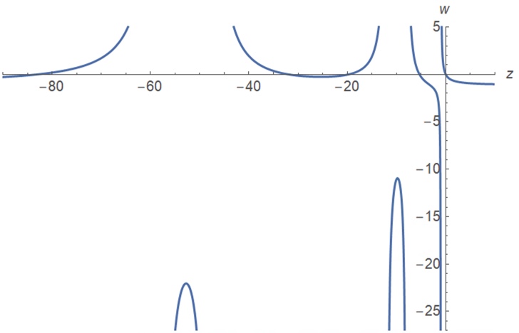
The restriction of to has zeroes and simple critical points, provided that is small enough. Moreover, the value of at each real critical point is strictly negative.
The graph of is represented in Figure 8, for .
Proof.
Let us first show that has real zeroes. Since the limit of on both extremities of each interval is for , the inequality implies the existence of real zeroes on each such interval. To ensure that these inequalities hold, observe that
and consequently that for any , we have
For , it implies that
and in turn that the value satisfies the sought inequality, for small enough.
This provides us with many real zeroes. Each of the intervals , contains a zero since
The remaining zero is at . In total, it provides us with real zeroes.
Let us now prove that has real simple critical points. First, we claim that the restriction of to each of the intervals of
has a global extreme value which is strictly negative. For , the claim follows from the fact that
For each remaining interval , the claim follows from the fact that
and the location of the real zeroes determined above.
It remains to show that each such extreme point is simple and that has no other real critical point, for small enough. To see this, recall that by Riemann-Hurwitz formula, exactly critical points of collapse at when tends to , for . Indeed, the degree of drops by since exactly two poles disappear, namely and , and the degree of the ramification divisor of drops therefore by . We claim that for small enough, exactly two of these ramification points are among the real critical points of exhibited above and the remaining two are complex conjugated. Moreover, there is no other real critical point since the function is -to- when .
In order to prove the above claim, it suffices to let all the , with , tend to and study the distribution of the remaining critical points. In other words, it amounts to consider the case , in particular . Then, we have
where we substituted . In order to study the behaviour of the ramification points of converging to when tends to , we need to analyse the singularity of the numerator of in the variables at . Since is a strictly negative number, we deduce that the latter singularity has Newton diagram with vertices , and and corresponding truncation . By the Newton-Puiseux theorem, we deduce that the singularity consists of two real branches parametrised respectively by and . For and arbitrarily small, the line intersects the first branch in one real point and the second branch in one real point and two complex conjugated points. The result follows. ∎
Remark 5.2.
As we have seen in the above proof, there are exactly two real critical points of in an arbitrarily small neighbourhood of each point for . Moreover, those two critical points, let us say and , are such that , see Figure 8.
Proposition 5.3.
The preimage of under is the union of with pairwise disjoint smoothly embedded circles in , provided that is small enough. Each such circle intersects at the real critical points and of near , for some .
Lemma 5.4.
Let be a real meromorphic function on a compact Riemann surface . Then, the preimage is a union of smoothly immersed circles such that each circle (respectively circles) self-intersects (respectively intersect) at worst transversely. Moreover, the set cannot contain a smooth open arc such that is a single point which is critical for .
Proof.
Fix an arbitrarily chosen Riemannian metric on and denote by the unitary tangent bundle with respect to the latter metric. Fix on orientation on . Then, the -fold inherits an orientation on its smooth locus and therefore lifts to . Since the local model of at singular points is , the closure of this lift is a smooth compact oriented -fold covering . Thus, the set is a disjoint union of smoothly embedded circles in . The restriction of the projection from to is a smooth immersion. The transversality property follows from the local models .
For the second part of the statement, the function is monotone on each smooth arc . In particular, the image under of the two extremities of are necessarily distinct points in . It prevents the existence of an arc as in the statement. ∎
Proof of Proposition 5.3.
For any small , we can choose small enough such that is contained in
Indeed, for any point , the image depends continuously on the parameters . When for all , the function satisfies as we have seen above. This proves the claim.
By the Riemann-Hurwitz formula, we showed above that we can also guarantee that there are exactly simple critical points of in each neighbourhood , , taking small enough. Moreover, exactly simple critical points are located on and the rest of the ramification consists of simple critical points that are complex conjugate.
By Lemma 5.4, the set consists of a union of smoothly immersed circles. Since there are exactly real simple critical points in , there is exactly one circle of in that intersects . This circle cannot pass through the remaining critical points in , otherwise it would contain the kind of smooth arc prohibited by Lemma 5.4. It follows that this circle is smoothly embedded. Eventually, we claim that there are no extra circles in . Indeed, any extra circle should be contain in one of the halves of for some . By Lemma 5.4, it cannot pass through the only critical point of in this half, otherwise it would contain an arc . It is therefore smooth and cover at least once via . This is in contradiction with the fact that has only real zeroes. ∎
For a given parameter , define , that is
| (13) |
where the real parameters are as in (12). The curve can be parametrised by
and the logarithmic Gauss map is given by
Let be the composition of with the parametrisation . In the affine chart of , the map is given by
Proposition 5.5.
For and small enough, the preimage is smooth and has connected components: one of the connected components contains the points
Each of the remaining components contains exactly one of the points .
Before proving the above statement, let us recall some basic facts from Morse theory. Let be a real analytic functions and let be a non-degenerate Morse critical point of index of such that . In particular, the zero locus of at consists of two branches intersecting transversely. Assume now that . Then, it follows from the Morse Lemma with parameters that, for any arbitrarily small , the zero locus of is smooth at . The local deformation of depends on the sign of , see Figure 9.
Recall as well that the imaginary part of a holomorphic function has non-degenerate Morse critical point of index at any simple critical point of . Indeed, up to an appropriate change of coordinate on the source, we can assume that the critical point under consideration is and that is given by whose Hessian in the coordinate is .
Proof.
First, observe that every and is a pole of , that and that . Therefore, each of these points belongs to .
Write where . Then, the locus is a real algebraic curve in the -plane that depends algebraically on the parameter . Indeed, the latter locus is the zero set of . For , that is , the real algebraic curve in the -plane consists of the union of the line with mutually disjoint smooth ovals, by proposition 5.3. Each oval intersects in exactly points and is symmetric with respect to . By Remark 5.2, we can localise the latter pair of points for each oval. In particular, the locus is as pictured on the top of Figure 10. Moreover, we have that the imaginary part of is negative on the complement component of that contains since . Therefore, the sign of is as pictured on top of Figure 10.
If we denote and , we have that . On the -axis, the function is real valued so that . Since is strictly negative at its real critical points, that these critical points are located on , by Proposition 5.1, then is strictly positive at the critical points of . Therefore, we can determine which of the two possible deformations of Figure 9 applies at each critical point of to obtain the locus . The latter locus is picture on the bottom of Figure 10 for . The case is obtianed by flipping the latter picture upside down. The result follows. ∎
6. Proof of Theorem B
Lemma 6.1.
For any choice of real parameters as in (12) and with small enough absolute value, the polynomial
| (14) |
is such that is connected.
Proof.
For , the curve is a simple Harnack curve. To see this, observe that the coordinate gives a parametrisation of and that the points of intersection of the closure of in with the toric divisors are parametrised by . In particular, these points are in maximal cyclical position according to [Mik00, Definition 2] and is therefore a simple Harnack curve. As a consequence, the Log-critical locus is smooth and connected since is rational. Eventually, the set remains smooth and connected for small . ∎
Proof of Theorem B.
In order to prove the statement, we will apply Theorem A to a specific Viro polynomial constructed from a degree polynomial and a -convex function . We choose in such a way that the induced subdivision of is the one pictured in Figure 11. The latter subdivision consists of sub-polygons defined as and sub-polygons defined as for and . This is clear that such a function exists.
We will now construct the polynomial , up to an irrelevant multiplicative constant. To do so, it suffices to describe for each the algebraic curve in defined by the truncation .
We fix an given integer as in the statement. Let denote the integer such that , and .
We now start the construction on . If , we fix to be the curve defined by any equation of degree as in (13). If , we fix to be the curve defined by an equation of degree where is as in (13). To ensure the compatibility of with along the edge , we need to take the parameters of to be the parameters of . We keep on with the same procedure up to included.
It should be clear by now that we can inductively define the curves , , using a polynomial as in either (13) or (14), adjusting the parameters of this curve to the parameters of the curve beneath it, using a change of variable if necessary. Then, we define any curve , , using a polynomial as in (14) and , if , using a polynomial as in (13).
For the curves , , we use toric translations of the simple Harnack curve . We first choose to be a toric translation of compatible with along (there is a -family of such). Next, we choose to be the unique toric translation of compatible with both and . We keep on with the same procedure up to . Eventually, we pick to be any line compatible with . Since the curve is smooth with smooth Log-critical locus for any , the corresponding Viro polynomial is Log non-degenerate.
We now define for where is the open set provided by Theorem A. We claim that . First, consider the patchwork obtained by throwing away the -s. For any , the Log-critical locus consists of one component intersecting the divisor and components intersecting , according to Lemma 5.5. After patchworking, each of the components connects to the component of intersecting , included. We obtain components this way. The patchwork of the loci , provides us with a single component intersecting and as many compact components in as there are lattice points in the interior of . Similarly the patchwork of the of the loci , provides us with a single component intersecting and as many compact components in as there are lattice points in the interior of . In total, we obtain as many compact components as the number of lattice points in the interior of minus the number of lattice points in the interior of the segment , that is
To conclude, we reintroduce the polygons in the patchwork. All the previous components intersecting are now connected to each other and form a single connected component of . There are new compact components in . In total, we obtain components. ∎
7. Appendix
In this last section, we illustrate the necessity of the assumption of Theorem C. Namely, we provide an example of Viro polynomial that is Log degenerate and show that the tropical limit of some Log-inflection points is not as predicted by the latter theorem. Below, we use the notations of Section 4.
Consider the Viro polynomial
whose coefficients depends on the complex parameters , , and . Consider for a moment the polynomial . Since is a factor of the truncations of to and respectively, the point is a singular point of the Log-critical locus , as hinted in the proof of Lemma 4.1(c). In particular, the latter point is a Log-inflection point. Therefore, the Viro polynomial is Log degenerate. However, it is non-degenerate for a generic choice of the coefficients , , and .
The Riemann-Hurwitz formula implies that there are exactly 3 Log-inflection points in for small values of . Repeating similar computations as in Section 4, we can provide a parametrisation for the latter points.
The polynomial is given by
with Newton polygon . Plainly, the numerator does not depend on since itself does not depend on . Its Newton polyhedron is therefore contained in the -plane and is actually given by . The truncation of to the edge is . It follows that is a tropism of the ideal since it is orthogonal to the edge of and the edge of . The corresponding solutions of the system , which are Log-inflection points of the curve , are parametrised by
| (15) |
in the -coordinates. The composition of this parametrisation with each of and is identically zero. This leads to two equations on the coefficients and that are eventually equivalent to
Using the substitution in the solutions (15) and switching back to the coordinates gives the following parametrisation for the Log-inflection points
Thus, the tropical limit of the 3 corresponding Log-inflection points is the point , lying on the edge of the tropical limit.
Observe that further computations lead to the formula
In turn, this formula allows to describe the Log-critical locus of in terms of the Log-critical loci of and for small and generic.
References
- [BIMS15] E. Brugallé, I. Itenberg, G. Mikhalkin, and K. Shaw. Brief introduction to tropical geometry. In Proceedings of the 21st Gökova geometry-topology conference, Gökova, Turkey, May 26-30, 2014, pages 1–75. Somerville, MA: International Press; Gökova: Gökova Geometry-Topology Conferences (GGT), 2015.
- [BKS16] D. V. Bogdanov, A. A. Kytmanov, and T. M. Sadykov. Algorithmic computation of polynomial amoebas. In Computer algebra in scientific computing, volume 9890 of Lecture Notes in Comput. Sci., pages 87–100. Springer, Cham, 2016.
- [GKZ08] I.M. Gelfand, M.M. Kapranov, and A.V. Zelevinsky. Discriminants, resultants, and multidimensional determinants. Reprint of the 1994 edition. Modern Birkhäuser Classics. Boston, MA: Birkhäuser. x, 523 p., 2008.
- [GLS18] G.M. Greuel, C. Lossen, and E. Shustin. Singular algebraic curves. With an appendix by O. Viro. Cham: Springer, 2018.
- [Har76] A. Harnack. Ueber die vieltheiligkeit der ebenen algebraischen curven. Mathematische Annalen, 10(2):189–198, 1876.
- [Lan15] L. Lang. A generalization of simple Harnack curves. ArXiv: 1504.07256, April 2015.
- [Lan19] L. Lang. Amoebas of curves and the Lyashko-Looijenga map. J. Lond. Math. Soc., II. Ser., 100(1):301–322, 2019.
- [Lan20] L. Lang. Harmonic tropical morphisms and approximation. Mathematische Annalen, 377(1):379–419, 2020.
- [Mau80] J. Maurer. Puiseux expansion for space curves. Manuscr. Math., 32:91–100, 1980.
- [Mik00] G. Mikhalkin. Real algebraic curves, the moment map and amoebas. Ann. of Math. (2), 151(1):309–326, 2000.
- [MR18] G. Mikhalkin and A. Renaudineau. Tropical limit of log-inflection points for planar curves. Sbornik: Mathematics, 209(9):1273, 2018.
- [Ris93] J.J. Risler. Construction d’hypersurfaces réelles (d’après Viro). In Séminaire Bourbaki. Volume 1992/93. Exposés 760-774 (de 1948/49 à 1992/93), pages 69–86. Paris: Société Mathématique de France, 1993.
- [Til05] S. Tillmann. Boundary slopes and the logarithmic limit set. Topology, 44(1):203–216, 2005.
- [Vir84] O.Ya. Viro. Gluing of plane real algebraic curves and constructions of curves of degrees 6 and 7. Topology, general and algebraic topology, and applications, Proc. int. Conf., Leningrad 1982, Lect. Notes Math. 1060, 187-200 (1984)., 1984.