Advanced control based on Recurrent Neural Networks learned using Virtual Reference Feedback Tuning and application to an Electronic Throttle Body (with supplementary material)
Abstract
In this paper the application of Virtual Reference Feedback Tuning (VRFT) for control of nonlinear systems with regulators defined by Echo State Networks (ESN) and Long Short Term Memory (LSTM) networks is investigated. The capability of this class of regulators of constraining the control variable is pointed out and an advanced control scheme that allows to achieve zero steady-state error is presented. The developed algorithms are validated on a benchmark example that consists of an electronic throttle body (ETB).
I Introduction
Nowadays, data science is increasingly spreading due to the recent introduction of innovative tools and algorithms for extracting information from data [1].
In the recent decades, data-based identification and control techniques [2] have been subject of increasing attention in research. In automation and control, several approaches are devoted to indirect data-based methods for control design that aim at first identifying a model of the plant, based on which the controller is then designed [3]. The plant model is identified by means of linear structures, e.g. ARX (AutoRegressive models with eXogenous variables), or nonlinear ones, e.g. Hammerstein-Wiener models or Recurrent Neural Networks (RNN) [4].
On the other hand, direct data-based methods for control design provide a valid alternative to indirect methods. In this case, the controller is directly identified through optimization from a controller class previously selected without preliminarily using the data to identify a model of the plant. They are either based on a reference model, e.g. Virtual Reference Feedback Tuning (VRFT) [5], Iterative Learning [6], or they exploit more recent model-free techniques, e.g. based on Reinforcement Learning [7].
In particular, VRFT has been first introduced for linear controller design [8] and then has been extended to nonlinear controller classes [9]. The use of VRFT to tune controllers of the class of Neural Networks (NN) has been marginally investigated. In [10] and [11], the filter implementation in the training algorithm of RNNs using dynamic backpropagation of the gradients is discussed and applied to a simulated crane model. In [12], VRFT is applied to Multi-Input–Multi-Output (MIMO) nonlinear systems using a three-layer neural network controller trained by least squares. Finally, in [13], this method is used for tuning fractional order (FO) and state-feedback NN controllers.
Among NNs, it has been proved that RNNs have promising capabilities in modeling and control of nonlinear systems [14]. Among RNNs, Echo State Networks (ESN) [15] and Long Short Term Memory (LSTM) networks [16] are particularly advantageous since they do not suffer from the vanishing gradient problem [17], an issue occurring during the training of recurrent networks in case the gradients of the network output with respect to the parameters in the early layers become very small. Moreover, as discussed in [18] and in [19] (dealing with ESNs and LSTMs, respectively), some notable properties of these classes of RNNs (i.e., ISS [20]) can be easily studied and even enforced during the training phase.
In this paper, we focus on the application of VRFT for controller design, with attention to regulators with ESN and LSTM structures.
The use of these networks has a twofold advantage: first, we can safely enforce stability-related properties to the controller; secondly, thanks to the nonlinear structures of these RNNs, we can explicitly enforce constraints on the control variables by constraining the networks parameters in the learning phase. The latter is a remarkable advantage over other commonly-used controller structures, since in most applications the control variables are bounded in defined ranges. Among direct methods, only in [21] an alternative is provided by means of a hierarchical control architecture, where an inner controller is first designed to match an a-priori closed-loop model and an outer model predictive controller is synthesized to consider input/output constraints and to enhance the performance of the inner loop.
In the advanced control scheme proposed in this paper, steady-state performance is guaranteed by suitable explicit integral actions. In this work, for notational simplicity (and in view of the fact that the considered case study has one input and one output), we consider single-input and single-output (SISO) networks, although a generalization to multiple-input and multiple-output systems is straightforward.
A case study consisting of an electronic throttle body (ETB) [22] is considered to validate the proposed control strategies.
The paper is organized as follows: Section II shortly recalls the Virtual Reference Feedback Tuning method for the design of nonlinear SISO systems, Section III shows the equations of the regulators defined by ESNs and LSTMs. Also, in Section IV the advanced control scheme used for control of the ETB is presented. Finally, Section V discusses the application to the benchmark example, while conclusions are drawn in Section VI.
II Virtual Reference Feedback Tuning
In this section a brief overview on VRFT is given. VRFT (see, e.g., [5, 8, 9]) is a direct data-based controller design method, i.e., where a batch of data is commonly sufficient to obtain a controller and no iterations are necessary. Considering Figure 1, the objective of VRFT is to identify a controller (with unknown parameter vector ), such that the resulting closed-loop system is as similar as possible to a given reference closed-loop model M for a given reference of interest.

This is done using, as available data, input and output sequences of length drawn from the plant. In this paper we consider the noise-free case, since in the considered case study noise is practically negligible (see Section V). If necessary, noisy data can be easily dealt with, e.g., using instrumental variable methods (as suggested in [9]).
The main idea behind VRFT is to compute the optimal value of the unknown controller parameter vector that solves the following problem:
| (1) |
where is the output sequence obtained by using the controller and is the Euclidean norm. If is sufficiently rich and is sufficiently exciting, solving (1) allows to obtain a controller that makes the closed-loop system as close as possible to M. However, the optimization problem (1) cannot be formulated in practice, since the plant model is not known. Therefore, the so-called virtual reference sequence consistent with the output sequence is computed according to
| (2) |
The sequence is denoted as virtual because it does not exist in reality and it was not in place when data and were collected. It is indeed the reference signal that, if injected at the feedback control system input, it produces as output in accordance with . It is possible to define as the virtual error and to identify the optimal value of vector by minimizing the following alternative P-free cost:
| (3) |
where is a suitable filter. For simplicity, in the following we assume . A good controller is one that produces when fed by because, through P, this generates , the desired output when reference is .
The objective reference map M can be selected as a general nonlinear system. In this work, in order to impose performances in a simple way, we use a linear system. We must select as invertible, in such a way that we can compute the sequence of reference values given the sequence of output values as in (2).
Concerning the controller class , it may be selected as a class of linear systems (e.g. PID controllers) or nonlinear ones. In this paper we will focus our attention on some notable classes of RNNs, in view of their notable properties, discussed in the following section.
III RNN regulators
In this section the equations of the RNN regulators that will be used as controller class are defined, as well as the properties that can be guaranteed through suitable constraints on the unknown parameters.
III-A ESN regulators
III-A1 Regulator equations
Starting from the equations defined by Jaeger in [15], it is possible to obtain the non-strictly proper version (to avoid to include an unnecessary delay in the computation of the control action) of the ESN equations, that will be used for the controller. We consider an ESN regulator with neurons (i.e. states ) in the reservoir, input and output . Upstream we apply a suitable input scaling and shift thanks to parameters and , respectively, i.e.,
| (4a) | ||||
| The dynamics of the ESN is described by the equations | ||||
| (4b) | ||||
| (4c) | ||||
| where is the so-called activation function. In the SISO case , , , , and . Finally, the following downstream de-normalization is applied, thanks to scaling and shift parameters and , respectively. | ||||
| (4d) | ||||
Importantly, the tuning of Echo State Networks is computationally advantageous over other types of RNNs. Indeed, while the choice of matrices , , and in the dynamic equation (4b) is largely arbitrary (although they can be subject to optimizaton using, e.g., the approach developed in [24]), matrices and are estimated based on a suitable least square-based optimization algorithm (see, e.g., [18]). Since the equation (4c) is linear-in-the-parameters, the identification algorithm boils down to a computationally lightweight quadratic program. This, as a byproduct, makes it possible to straightforwardly apply instrumental variable methods when dealing with noisy data, as discussed in [23].
III-A2 Constrained inputs
With reference to the ESN regulator (4), the following property holds.
Property 1. Consider an ESN regulator defined by equations (4), with . If in (4c), then
| (5) |
Recall that, given a matrix with elements , is its -norm, i.e., .
Proof:
Consider the output equation of an ESN regulator (4c). If , the equation becomes:
Since element-wise,
and so . Recalling (4d), we obtain (5). ∎Remark 1. Property 1 can straightforwardly be extended to a MIMO regulator and in particular each component of the input vector is bounded in a similar way. The only difference lies in how inputs and outputs are normalized and de-normalized, since each element of the input and output vectors can be subject to different scaling operations.
Based on (5), a regulator with a control variable constrained in a range [,] can be obtained as follows:
- 1.
Fix the output shift and scaling parameters, i.e.,
(6) - 2.
It is finally worth noting that, based on the results presented in [18], it is possible to provide an analytical sufficient condition for guaranteeing that the ESN enjoys -ISS [20], i.e., . The latter condition can be explicitly enforced in the optimization problem (7) as a further constraint. In the experimental results illustrated in Section V, however, this condition turns out to be rather restrictive for the selection of suitable controllers. In view of this, we opted to remove this condition from the optimization problem, while checking a posteriori suitable stability-related properties of the resulting regulator, as described later in the paper.
III-B LSTM regulators
III-B1 Regulator equations
Starting from the equations defined by Hochreiter Schmidhuber in [16], it is possible to obtain the nonstrictly proper version of the LSTMs. We define and and, when applied to a vector, we assume to apply them element-wise. Furthermore, ‘’ represents the element-wise (Hadamard) product. We consider an LSTM regulator with hidden layers, input and output . Upstream we apply the input scaling (4a). The dynamics of the LSTM is described by the equations
| (8a) | ||||
| (8b) | ||||
| (8c) | ||||
| where is the forget gate, the input gate, the input activation, the output gate, , , , . Finally, the downstream de-normalization (4d) is used. | ||||
III-B2 Constrained inputs
For LSTM regulators (8), the following property holds.
Property 2. Consider an LSTM regulator defined by equations (4a), (8), and (4d), with . The output is bounded as follows
| (9) |
Proof:
Since, in view of their definitions, and element-wise, then as defined in equation (8b). Hence, considering (4d), it is possible to write:
It is worth noting that Remark 1 also applies to LSTM regulators, i.e., the extension to MIMO systems is straighforward.
Based on (9), a regulator with a control variable constrained in a range [,] can be obtained as follows:
- 1.
Fix the output shift and scaling parameters according to (6).
- 2.
Defining with the vector of tuning parameters, solve the following nonlinear constrained optimization problem
(10) subject to
where is the output data vector and is the predicted output data vector, both normalized.
Similarly to the case of ESNs, it is possible to provide an analytical sufficient condition for guaranteeing that the regulator enjoys -ISS, i.e., that a suitably-defined matrix is Schur stable [26]. Also in this case, being such condition only sufficient, it provided an overly-conservative constraint when used in (10). For this reason in Section V, the stability-related properties of the LSTM are checked a posteriori.
IV Control scheme
The advanced control scheme shown in Figure 2 will be used in the case study in order to achieve zero steady-state error and to bound the control variable avoiding the wind-up phenomenon. In particular, an anti wind-up integrator is placed in parallel (also when generating the data for the training of the RNN regulators) to the constrained ESN or LSTM regulator and, provided that the closed-loop system is asymptotically stable, a null steady-state error is guaranteed.

In this case, , where and are the inputs generated by the integrator and the RNN, respectively. The gain of the integrator is chosen so as to take into account the different orders of magnitude of the error and the control variable.
The anti wind-up block is indeed used to effectively bound the input variable. If the control variable has to be bounded in a range [], then the additive components and must be bounded in such a way that is in the requested interval. In particular, we define in such a way that
and we will bound (the integrator output) and (the RNN output) in a “differential” way, i.e. by setting and . The definition of the bounds for and is a design choice and depends on a trade-off: the wider the range of , the wider the range reachable by at steady-state but narrower the range of action of the RNN regulator which is exerted during the transient. Conversely, if a narrow range for is chosen, the RNN regulator has a wider freedom of exerting its regulatory action but at steady-state turns out to be bounded in a narrow interval.
Since the limits of the saturation and are established before the training phase, we must keep in consideration the effect of the anti wind-up block also in the training phase. More in details, the training of the RNN is done by using as input and as output, where
V Experimental results
V-A System description and experimental setup
The proposed controllers are validated on the electronic throttle body (ETB) depicted in Figure 3.

The ETB is composed of four throttle valves actuated by a DC brushed motor, equipped with a planetary reduction gear and a connectiong rod which links the shaft of the motor to the shaft of the four valves. The input of the system is a voltage, obtained through a 20 kHz PWM signal, constrained in the range V. The output is the throttle shaft position measured by an angular potentiometer and defined in the range (0 means that the valve is completely closed and 1 that it is totally open). The ETB is a nonlinear SISO system whose nonlinearities are mainly due to friction phenomena and to the nonlinear spring stiffness.
V-B Setting and available data
A sample time s is chosen for the data acquisition and the controller triggering. Since the settling time is equal to when the maximum or minimum step of voltage is applied, a reasonable specification for the settling time of the closed-loop system is . This corresponds with the following unitary gain reference model: , where we set and .
The available data are obtained with a Multilevel Pseudo-Random Signal (MPRS), [3]: half with switching period and half with switching period . The amplitude of the PWM is in the range V so as to have the throttle shaft position covering the whole range of interest . Figure 4 shows a portion of the data acquired from the ETB: note that, consistently with the assumption done in Section II, noise on the data can be neglected.

V-C Controller identification
The applied control scheme is the one described in Section IV with two alternative RNN regulators, i.e., a ESN and a LSTM. The gain of the integrator is set equal to and the saturation limits of the integrator are V and V, allowing to reach all the throttle shaft positions in the range at steady-state. The ESN and LSTM regulators are bounded in the range V: this makes it possible to bound the control variable in the range V.
The training of the RNN regulators is carried out using as input and as output.
The ESN regulator is trained as in [18] setting according to the algorithm in Section III, i.e. by means of the ESN learning toolbox developed by Jaeger [15] and by means of YALMIP [25].
The LSTM regulator is trained according to the algorithm in Section III by means of the MATLAB function fmincon and the implementation of the backpropagation through time (BPTT) algorithm, setting . Inspired by the LSTM variants discussed in [27], and in order to lighten the computational burden in the training of LSTM in the constrained case, we have set and in such a way that the network in (8) takes the following simplified form:
We also set , naturally verifying and . In this case the minimization is performed with respect to the matrices only.
The fitting parameter used to evaluate the quality of the identification procedure is
| (11) |
where is the acquired control variable, is the control variable simulated by the network and is the mean value of the acquired control variable . In Figure 5, a portion of the validation data of the ESN and LSTM regulators is depicted.

The fitting value achieved by the ESN regulator is , while the one obtained by the LSTM regulator is .
Finally, as discussed in Sections III-A2 and III-A2, the stability properties of the considered regulators are not imposed during the training phase. However, we have successfully numerically verified a posteriori the asymptotic stability of the equilibria corresponding with the static characteristic curves of both regulators (see Figure 6).

V-D Reference tracking results
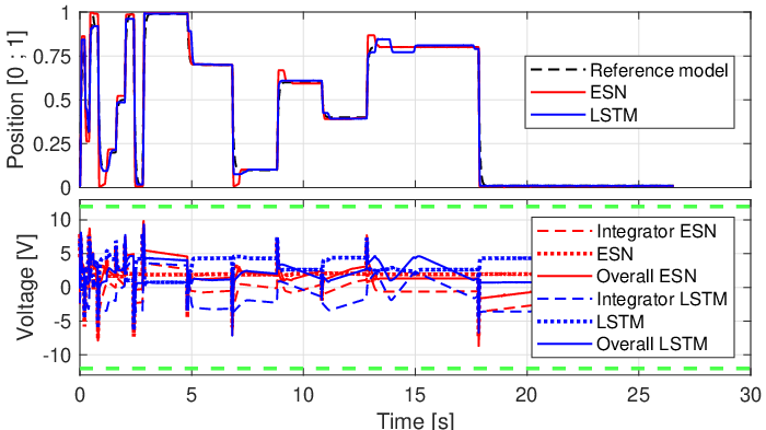
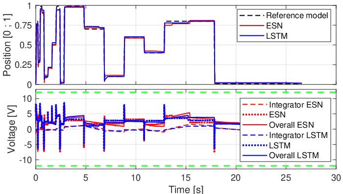
A time-varying reference position signal is used in these tests. In Figure 7, the reference tracking results are shown for the considered RNN regulators, while for better insight the reference output error is shown in Figure 8. In the upper plot of Figure 7, the reference closed-loop model output is depicted with a black dashed line, the system output with an ESN regulator is displayed with a red line and the system output with a LSTM regulator with a blue line. The bottom plot shows , and when ESN and LSTM regulators are used, respectively.


V-E Comparisons with different setups
In this section the previous constrained RNN regulators are compared with other RNN regulators designed according to different design choices. These results are shown to motivate the adopted design choices, as well as the role of constraints in the tuning of the RNN and of the integrator.
V-E1 Different reference model
In Figure 9 we show the reference tracking results of the RNN regulators when the reference closed-loop model has settling time equal to , i.e., where , . In this case, the fitting index of the ESN regulator is equal to with , while the one of the LSTM regulator is with . It is possible to notice that the tracking performances are slightly worse with respect to the ones obtained in the case illustrated in Section V-D. In particular, as apparent from Figure 10, the closed-loop responses now display smaller overshoots with respect to the case in Section V-D, but at the price of longer transients.

V-E2 Different integrator weight
Figure 11 shows the reference tracking results of the constrained RNN regulators in parallel to a constrained integrator when the reference closed-loop model has settling time equal to but the gain of the integrator is equal to . The fitting of the ESN regulator is equal to with , and the one of the LSTM regulator is with . It is possible to notice from Figure 12 that, due to the smaller gain of the actuator, the latter is less responsive than in the case considered in Section V-D, where . In view of this, the final transients of the closed-loop response are slower.

V-E3 Constrained network tuning and no integrator
Figure 13 shows the reference tracking results of the constrained RNN regulators applied without any integrator in the loop. The settling time of the reference closed-loop model is set to , the fitting of the ESN regulator is equal to with , and the fitting of the LSTM regulator is equal to with . Despite the tracking results in Figure 13 appear to be rather promising, from an inspection of Figure 14 we can observe that the static precision of the control system is not perfect (i.e., the responses display non-zero steady-state errors). This is due to the unavoidable regulator identification inaccuracies and highlights the importance of including suitable integral actions in the loop.


V-E4 Unconstrained network tuning and integrator


In Figures 15 and 16 the reference tracking results of the unconstrained RNN regulators applied with an unbounded integrator in the loop (with gain and , respectively) are represented. The settling time of the reference closed-loop model is set to , the fitting of the ESN regulators with are equal to in both cases, and the fitting of the LSTM regulators with are equal to and , respectively. In Figures 17 and 18 the reference output errors with the LSTM regulators are shown in the two considered cases, respectively.
In the first case, i.e. when , it is possible to observe that several equilibria are not asymptotically stable, especially when the ESN regulator is applied. On the other hand, in the second case, i.e. when , the response exhibits problems in reaching a zero steady-state error since the integral action is not sufficiently effective, especially with the ESN regulator.
However, the lack of control variable constraints makes the inclusion of an integral action in this scheme critical, as the integrator could generate indefinitely high values of the control variable and there are no guarantees that the output of the RNN regulators does not exceed the control variable limits. In particular, since the position error in the considered case study, the output of the ESN regulator (4) with is bounded as follows:
| (12) |
Hence, the output of the ESN regulator turns out to be bounded in V if and in V if . On the other hand, according to (9), the LSTM regulator turns out to be bounded in V if and in V if . Note that, indeed, the LSTM regulators perform better than the ESN ones.
V-E5 Unconstrained network tuning and no integrator
Finally, in Figure 19 the reference tracking results of the unconstrained RNN regulators applied without any integrator in the loop are depicted. In this case the settling time of the reference closed-loop model is . The fitting of the ESN regulator is equal to with , while the one of the LSTM regulator is with . Regarding the ESN, the system response is highly unsatisfactory because the control variable often exceeds the saturation limits (the green dashed line represents the PWM limits). This underlines the practical importance of explicitly imposing input variable constraints in the regulator tuning. On the other hand, the response of the LSTM is less critical because it only exhibits problems in reaching a zero steady-state error when the values of the reference signal are close to 1. However, also in this case, there are no guarantees that the output of the RNN regulators does not exceed the control variable limits. According to (12), the ESN regulator is bounded in V. Instead, according to (9), the LSTM regulator is bounded in V.

VI Conclusions
This paper describes the application of the VRFT method for control of nonlinear SISO systems with regulators described by ESNs and LSTMs. Their capability to constrain the control variable is pointed out and an advanced control scheme that allows to achieve a zero steady-state error is devised. Experimental results that validate the developed algorithms are shown considering a real ETB system.
Future works concern the comparison with other direct or indirect data-based methods and the extension of the developed control strategies to MIMO systems. Also, we will investigate how alternative choices of the reference model (including nonlinear ones) may affect the performances of the control systems.
References
- [1] X. Wu, et al., “Top 10 algorithms in data mining.” Knowledge and information systems 14.1 (2008): 1-37.
- [2] A. Aswani, H. Gonzalez, S. S. Sastry, and C. Tomlin, “Provably safe and robust learning-based model predictive control.” Automatica 49.5 (2013): 1216-1226.
- [3] L. Bugliari Armenio, E. Terzi, M. Farina, and R. Scattolini, “Echo State Networks: analysis, training and predictive control.” 2019 18th European Control Conference (ECC). IEEE, 2019.
- [4] C. M. Lin, and C. F. Hsu, “Recurrent-neural-network-based adaptive-backstepping control for induction servomotors.” IEEE Transactions on industrial electronics 52.6 (2005): 1677-1684.
- [5] A. Lecchini, M. C. Campi, and S. M. Savaresi, “Virtual reference feedback tuning for two degree of freedom controllers.” International Journal of Adaptive Control and Signal Processing 16.5 (2002): 355-371.
- [6] S. Gunnarsson, O. Rousseaux, and V. Collignon, “Iterative feedback tuning applied to robot joint controllers.” IFAC Proceedings Volumes 32.2 (1999): 4676-4681.
- [7] Y. Tange, S. Kiryu, and T. Matsui, “Model Predictive Control Based on Deep Reinforcement Learning Method with Discrete-Valued Input.” 2019 IEEE Conference on Control Technology and Applications (CCTA). IEEE, 2019.
- [8] M. C. Campi, A. Lecchini, and S. M. Savaresi, “Virtual reference feedback tuning: a direct method for the design of feedback controllers.” Automatica 38.8 (2002): 1337-1346.
- [9] M. C. Campi, and S. M. Savaresi, “Direct nonlinear control design: The virtual reference feedback tuning (VRFT) approach.” IEEE Transactions on Automatic Control 51.1 (2006): 14-27.
- [10] A. Esparza, A. Sala, and P. Albertos, “Neural networks in virtual reference tuning.” Engineering Applications of Artificial Intelligence 24.6 (2011): 983-995.
- [11] A. Esparza, and A. Sala, “Application of neural networks to virtual reference feedback tuning controller design.” IFAC Proceedings Volumes 40.21 (2007): 145-150.
- [12] P. Yan, D. Liu, D. Wang, and H. Ma, “Data-driven controller design for general MIMO nonlinear systems via virtual reference feedback tuning and neural networks.” Neurocomputing 171 (2016): 815-825.
- [13] M. B. Radac, and R. E. Precup, “Data-driven MIMO model-free reference tracking control with nonlinear state-feedback and fractional order controllers.” Applied Soft Computing 73 (2018): 992-1003.
- [14] T. W. Chow, and Y. Fang, “A recurrent neural-network-based real-time learning control strategy applying to nonlinear systems with unknown dynamics.” IEEE transactions on industrial electronics 45.1 (1998): 151-161.
- [15] H. Jaeger, “The “echo state” approach to analysing and training recurrent neural networks-with an erratum note.” Bonn, Germany: German National Research Center for Information Technology GMD Technical Report 148.34 (2001): 13.
- [16] S. Hochreiter, and J. Schmidhuber, “Long short-term memory.” Neural computation 9.8 (1997): 1735-1780.
- [17] A. Graves, “Long short-term memory.” Supervised sequence labelling with recurrent neural networks. Springer, Berlin, Heidelberg, 2012. 37-45.
- [18] L. Bugliari Armenio, E. Terzi, M. Farina, and R. Scattolini, “Model predictive control design for dynamical systems learned by echo state networks.” IEEE Control Systems Letters 3.4 (2019): 1044-1049.
- [19] E. Terzi, M. Farina, and R. Scattolini, “Model predictive control design for dynamical systems learned by Long Short-Term Memory Networks”. In: arXiv preprint arXiv:1910.04024 (2019).
- [20] D. Angeli, “A Lyapunov approach to incremental stability properties”. IEEE Transactions on Automatic Control, vol. 47, no. 3, pp. 410-421, March 2002.
- [21] D. Piga, S. Formentin, and A. Bemporad, “Direct data-driven control of constrained systems.” IEEE Transactions on Control Systems Technology 26.4 (2017): 1422-1429.
- [22] G. Panzani, M. Corno, and S. M. Savaresi, “On adaptive electronic throttle control for sport motorcycles.” Control Engineering Practice 21.1 (2013): 42-53.
- [23] W. D’Amico, “Direct nonlinear control design: virtual reference feedback tuning with recurrent neural networks.” Master Thesis, Politecnico di Milano, Academic Year 2018-2019.
- [24] L. Bugliari Armenio, L. M. Fagiano, E. Terzi, M. Farina, R. Scattolini, “Optimal Training of Echo State Networks via Scenario Optimization.” In Proceedings of IFAC World Congress, 2020.
- [25] J. Löfberg, J., “YALMIP : A Toolbox for Modeling and Optimization in MATLAB.” In Proceedings of the CACSD Conference, 2004.
- [26] E. Terzi, F. Bonassi, M. Farina, R. Scattolini, “Learning Model Predictive Control with Long Short-Term Memory Network.” arXiv:1910.04024, 2019.
- [27] K. Greff, R. K. Srivastava, J. Koutník, B. R. Steunebrink and J. Schmidhuber, “LSTM: A Search Space Odyssey.” IEEE Transactions on Neural Networks and Learning Systems, vol. 28, no. 10, pp. 2222-223.