Modularity and Mutual Information in Networks: Two Sides of the Same Coin

Qian Wang Affiliation: CFCS, Peking University Email: {charlie Yongkang Guo Affiliation: CFCS, Peking University Email: yongkang_guo Zhihuan Huang Affiliation: CFCS, Peking University Email: zhihuan.huang Yuqing Kong Affiliation: CFCS, Peking University Email: yuqing.kong}@pku

Abstract

Modularity, first proposed by Newman and Girvan 2004, is one of the most popular ways to quantify the significance of community structure in complex networks. It can serve as both a standard benchmark to compare different community detection algorithms, and an optimization objective to detect communities itself. Previous work on modularity has developed many efficient algorithms for modularity maximization. However, few of researchers considered the interpretation of the modularity function itself. In this paper, we study modularity from an information-theoretical perspective and show that modularity and mutual information in networks are essentially the same. The main contribution is that we develop a family of generalized modularity measures, $f$ -modularity based on $f$ -mutual information. $f$ -Modularity has an information-theoretical interpretation, enjoys the desired properties of mutual information measure, and provides an approach to estimate the mutual information between discrete random variables. At a high level, we show the significance of community structure is equivalent to the amount of information contained in the network. The connection of $f$ -modularity and $f$ -mutual information bridges two important fields, complex network and information theory and also sheds light on the design of measures on community structure in future.

1 Introduction

Networks have been attracting considerable attention over the past few decades as a representation of real data in many complex system applications, including natural, social, and technological systems. One of the most important characteristics that have been found to occur commonly in these networks is community structure Girvan and Newman 2002; Fortunato 2010; Porter et al. 2009; Malliaros and Vazirgiannis 2013; Cherifi et al. 2019. It is a natural idea to partition a complex network into multiple modules or communities by grouping nodes into sets such that each set of nodes are densely connected internally while cross-group connections are sparse. Therefore, research on community structure occupies an important part in data processing and data analyzing.

One of the most widely used tools for analyzing community structure is modularity Newman 2004. The modularity function is defined as

Q=\sum_{i}(e_{ii}-a_{i}^{2}),

where $e_{ij}$ denotes the fraction of edges connecting community $i$ to community $j$ (hence $e_{ii}$ for the edges within community $i$ ) and $a_{i}=\sum_{j}e_{ij}$ . In essence, modularity measures the “distance” of the community structure in the real network from a random network without any community structure, thus a higher modularity implies a clearer community structure. There has been extensive research on modularity-based techniques obtaining maximization algorithms with faster speed or higher accuracy. However, few work dived into the concept of modularity itself.

In this paper, we study modularity from an information-theoretical perspective and show that modularity and mutual information in networks are actually two sides of the same coin. By regarding the adjacency matrix of a network as the joint probability distribution of two discrete random variables, we observe an intuitive relation between mutual information and community structure. For example, if the adjacency matrix is a block diagonal matrix, there is naturally a good community partition with a high modularity for this network, while the value of mutual information is also high for this joint distribution at the same time.

Following this intuition, we start from $f$ -mutual information Kong and Schoenebeck 2019, a generalization of Shannon mutual information and derive a family of generalized modularity measures, $f$ -modularity. For a given network, when we consider the adjacency matrix as the joint probability matrix of two discrete random variables, maximizing $f$ -modularity is equivalent to approximating $f$ -mutual information. By substituting different convex functions $f$ , we can get different instances of $f$ -modularity. Actually, by picking a particular $f$ and adding some constraints, we will show that the original definition of Newman’s modularity is a special case of ours. For other commonly used smooth convex functions, $f$ -modularity surpasses Newman’s modularity due to it being differentiable.

The main contribution of this paper is proposing $f$ -modularity, which implies a strong connection between modularity and mutual information in networks. The key insight is that the significance of community structure equals the amount of information contained in the network. $f$ -modularity has an information-theoretical interpretation, enjoys the desired properties of mutual information measure, and provides an approach to estimate the mutual information between discrete random variables (Section 3). We validate our theoretical results by experiments in Section 4.

2 Related Work

Modularity was first proposed by Newman and Girvan 2004 as a stop criterion for another community detection algorithm. Then in the same year, Newman 2004 proposed an alternative community detection approach directly based on modularity maximization. They chose an greedy-based approximation algorithm in order to reduce time overhead. Later, modularity maximization was formally proved to be an NP-complete problem by Brandes et al. 2007.

Following the seminal work of Newman, many approximate optimization methods for modularity maximization were developed, offering different balances between lower complexity and higher accuracy Cherifi et al. 2019. Some researchers also aimed to address the shortcomings of modularity by proposing new metrics similar to modularity Muff et al. 2005; Haq et al. 2019. Instead of pursuing a better algorithm or making slight modifications to the original definition of modularity, we starts from $f$ -mutual information, entirely another concept, to derive a generalized modularity, which includes Newman’s modularity as a special case.

As far as we know, all previous work involving both Newman’s modularity and mutual information was related to normalized mutual information (NMF) Danon et al. 2005. NMF takes the partitions of the network as random variables while $f$ -mutual information in our context takes the edges of the network as random variables. Danon et al. 2005 first used NMF as a standard benchmark to compare different approaches for community detection, so later work on modularity just accepted it as a metric. Compared with them, we build a more solid mathematical connection between modularity and mutual information.

There is a only limit of literature looking into modularity itself and establishing its correspondences to other fields, but with no relevance to mutual information. Zhang and Moore 2014; Newman 2016; Veldt et al. 2018 showed the equivalence between modularity and the maximum likelihood formulation of the degree-corrected stochastic block models (SBM). Masuda et al. 2017 showed modularity is closely related to Markov stability in the random walk model. Chang et al. 2018 discussed the relation between modularity maximization and non-negative matrix factorization (NMF). Recently, Young et al. 2018 established the universality of the stochastic block model and showed all the problems where we partition the network by maximizing some objective function, are equivalent including modularity maximization.

3 $f$ -Modularity

In this section, we will provide the definition of $f$ -modularity based on the dual form of $f$ -mutual information. With different convex functions $f$ and constraint sets $C$ , we can get different instances of $f$ -modularity, one of which corresponds to Newman’s modularity. Finally, we illustrate an approximation algorithm to optimize $f$ -modularity.

3.1 Frequency Matrix and Random Matrix

This subsection formally describes our setting for networks. First, we define the frequency matrix of a network as follows.

Definition 3.1 (Frequency Matrix $\mathbf{F}$ ).

Given a bipartite multigraph $G=\left<U,V,E\right>$ and its biadjacency matrix $\mathbf{B}$ , where $B_{u,v}$ is the number of edges between $u\in U$ and $v\in V$ , the frequency matrix is defined as $\mathbf{F}=\mathbf{B}/N$ where $N=\sum_{u,v}B_{u,v}$ is the total number of edges. For a non-bipartite multigraph $G=\left<V,E\right>$ , given its adjacency matrix $\mathbf{A}$ , we define $\mathbf{F}=\mathbf{A}/N$ where $N=\sum_{u,v\in V}A_{u,v}$ .

Example 3.2 (Seller-Buyer).

$U$ is a set of sellers and $V$ is a set of buyers. For $N$ contracts, $B_{u,v}$ is the number of times that seller $u$ trades with buyer $v$ and $F_{u,v}=B_{u,v}/N$ .

Note that our work can be applied to both bipartite networks and non-bipartite networks, but we will mainly focus on bipartite networks since any adjacency matrix of a non-bipartite multigraph can be induced to the biadjacency matrix of a bipartite multigraph (see Figure 1 for illustration). In the following context, a “network”, if not particularly indicated, refers to a bipartite multigraph.

(a)

(b)

$\begin{pmatrix}0&1&1&0&0\\ 1&0&1&1&0\\ 1&1&0&0&1\\ 0&1&0&0&1\\ 0&0&1&1&0\end{pmatrix}$

(c)

Figure 1: The adjacency matrix of the non-bipartite graph in (1(a)) is exactly the same with the biadjacency matrix of the bipartite graph in (1(b)), i.e., the matrix in (1(c)). As the biadjacency matrix is symmetric in this situation, any rational algorithm should deliver a symmetric partition result for the bipartite graph (1(b)). For example, if the communities turn out to be

\{u_{1},u_{2},u_{3},v_{1},v_{2},v_{3}\}

and

\{u_{4},u_{5},v_{4},v_{5}\}

in the bipartite graph (1(b)), then we know the communities in the non-bipartite graph (1(a)) is

\{1,2,3\}

and

\{4,5\}

. Therefore, we only need to consider bipartite networks.

Next, we will define the random matrix (aka the null model). At a high level, modularity is a measure for the distance from the real network to the random network.

Definition 3.3 (Random Matrix $\mathbf{J}$ ).

Given a bipartite multigraph $G=\left<U,V,E\right>$ and its frequency matrix $\mathbf{F}$ , the random matrix $\mathbf{J}$ is defined as

J_{u,v}=(\deg(u)\deg(v)-\frac{1}{N}F_{u,v})\frac{N}{N-1},

where $\deg(u)=\sum_{j\in V}F_{u,j}$ is the normalized degree of vertex $u$ and similarly, $\deg(v)=\sum_{i\in U}F_{i,v}$ .

If the $N$ edges of $\mathbf{G}$ is $N$ i.i.d. samples of random variables $(X,Y)$ whose realizations are in $(U,V)$ , we have

	$\displaystyle\mathrm{E}[F_{u,v}]\quad$	$\displaystyle=\Pr[X=u,Y=v],$
	$\displaystyle\mathrm{E}[\deg(u)]$	$\displaystyle=\Pr[X=u],$
	$\displaystyle\mathrm{E}[\deg(v)]$	$\displaystyle=\Pr[Y=v].$

The following Lemma 3.4 tells us, $\mathbf{J}$ in Definition 3.3 is an unbiased estimation of $\Pr[X=u]\Pr[Y=v]$ .

Lemma 3.4.

$\mathrm{E}[J_{u,v}]=\Pr[X=u]\Pr[Y=v]$

Proof of Lemma 3.4.

Let

\mathrm{I}_{n}(u,v)=\left\{\begin{array}[]{ll}1&\text{if the }n\text{-th edge is }(u,v),\\ 0&\text{otherwise}.\end{array}\right.

Then

		$\displaystyle\sum_{i}F_{i,v}\sum_{j}F_{u,j}$
	$\displaystyle=$	$\displaystyle\frac{1}{N^{2}}\left(\sum_{i,n}\mathrm{I}_{n}(i,v)\right)\left(\sum_{j,n}\mathrm{I}_{n}(u,j)\right)$
	$\displaystyle=$	$\displaystyle\frac{1}{N^{2}}\left(\sum_{n}\mathrm{I}_{n}(u,v)+\sum_{n\neq n^{\prime}}\sum_{i,j}\mathrm{I}_{n}(i,v)\mathrm{I}_{n^{\prime}}(u,j)\right).$

We get

\mathrm{E}[\deg(u)\deg(v)]=\frac{1}{N}\Pr(u,v)+\frac{N-1}{N}\Pr(u)\Pr(v),

thus $\mathrm{E}[J_{u,v}]=\Pr[X=u]\Pr[Y=v]$ . ∎

3.2 $f$ -Divergence and $f$ -Mutual Information

This subsection introduces $f$ -divergence, Fenchel’s duality and $f$ -mutual information. These are the main technical ingredients for defining $f$ -modularity.

Definition 3.5 ( $f$ -Divergence Ali and Silvey 1966).

$f$ -Divergence $d_{f}:\Delta_{\Sigma}\times\Delta_{\Sigma}\mapsto\mathbb{R}$ is a non-symmetric measure of the difference between distribution $\mathbf{p}\in\Delta_{\Sigma}$ and distribution $\mathbf{q}\in\Delta_{\Sigma}$ and is defined to be

d_{f}(\mathbf{p};\mathbf{q})=\sum_{\sigma\in\Sigma}\mathbf{q}(\sigma)f\bigg(\frac{\mathbf{p}(\sigma)}{\mathbf{q}(\sigma)}\bigg),

where $f:\mathbb{R}\mapsto\mathbb{R}$ is a convex function and $f(1)=0$ .

As an example, by picking $f(t)=t\log(t)$ , we get KL-divergence $d_{KL}(\mathbf{p},\mathbf{q})=\sum_{\sigma}\mathbf{p}(\sigma)\log\frac{\mathbf{p}(\sigma)}{\mathbf{q}(\sigma)}$ .

Definition 3.6 (Fenchel Duality Rockafellar and others 1966).

Given any function $f:\mathbb{R}\mapsto\mathbb{R}$ , we define its convex conjugate $f^{\star}$ as a function that also maps $\mathbb{R}$ to $\mathbb{R}$ such that

f^{\star}(x)=\sup_{t}tx-f(t).

Lemma 3.7 (Dual Form of $f$ -DivergenceNguyen et al. 2010).

	$\displaystyle d_{f}(\mathbf{p};\mathbf{q})\geq$	$\displaystyle\sup_{u\in\mathcal{U}}\sum_{\sigma\in\Sigma}u(\sigma)\mathbf{p}(\sigma)-\sum_{\sigma\in\Sigma}f^{\star}(u(\sigma))\mathbf{q}(\sigma)$
	$\displaystyle=$	$\displaystyle\sup_{u\in\mathcal{U}}\mathrm{E}_{\mathbf{p}}u-\mathrm{E}_{\mathbf{q}}f^{\star}(u),$

where $\mathcal{U}$ is a set of functions that maps $\Sigma$ to $\mathbb{R}$ . The equality holds if and only if $u(\sigma)\in\partial{f}(\frac{\mathbf{p}(\sigma)}{\mathbf{q}(\sigma)})$ , i.e., the subdifferential of $f$ on value $\frac{\mathbf{p}(\sigma)}{\mathbf{q}(\sigma)}$ .

Function $u$ is a distinguisher between distribution $\mathbf{p}$ and distribution $\mathbf{q}$ and the best distinguisher $u^{*}$ (if not restricted by $\mathcal{U}$ ) maximizes the right side to be $d_{f}(\mathbf{p};\mathbf{q})$ . With the above lemma, we can also write the dual form as

d_{f}(\mathbf{p};\mathbf{q})=\sup_{D\in\mathcal{D}}\mathrm{E}_{\mathbf{p}}\partial{f}(D)-\mathrm{E}_{\mathbf{q}}f^{\star}(\partial{f}(D))

where $\mathcal{D}$ is a set of functions that maps $\Sigma$ to $\mathbb{R}$ and the best $D^{*}$ satisfies $D^{*}(\sigma)=\frac{\mathbf{p}(\sigma)}{\mathbf{q}(\sigma)}$ . Some common $f$ functions for $f$ -divergence and their dual forms are shown in Table 1.

Table 1: Reference Table for

f,f^{\star}

Kong and Schoenebeck 2019

$f$ -Divergence	$f(t)$	$\partial{f}(D)$	$f^{\star}(\partial{f}(D)$ )
Total Variation Distance	$\|t-1\|$	$\mathrm{sgn}(\log D)$	$\mathrm{sgn}(\log D)$
KL-Divergence	$t\log t$	$\log D+1$	$D$
Pearson $\chi^{2}$	$(t-1)^{2}$	$2(D-1)$	$D^{2}-1$
Jensen-Shannon	$-(t+1)\log{\frac{t+1}{2}}+t\log t$	$\log{\frac{2D}{1+D}}$	$-\log(\frac{2}{1+D})$
Squared Hellinger	$(\sqrt{t}-1)^{2}$	$1-\sqrt{\frac{1}{D}}$	$\sqrt{D}-1$

Definition 3.8 ( $f$ -Mutual Information Kong and Schoenebeck 2019).

Given two random variables $X,Y$ , the $f$ -mutual information between $X$ and $Y$ is defined as

	$\displaystyle\textsc{MI}^{f}(X;Y)=$	$\displaystyle d_{f}(XY;X\otimes Y)$
	$\displaystyle=$	$\displaystyle\sum_{x,y}\Pr(x)\Pr(y)f\left(\frac{\Pr(x,y)}{\Pr(x)\Pr(y)}\right)$

where $d_{f}$ is $f$ -divergence.

$f$ -Mutual information measures the correlation of two random variables $X$ and $Y$ via $f$ -divergence between the joint distribution, denoted as $XY$ , and the product of the marginal distributions, denoted as $X\otimes Y$ . As an example, by picking $f$ -divergence as KL-divergence, i.e., $f(t)=t\log t$ Cover 1999, we get the classic Shannon mutual information,

\textsc{MI}^{Shannon}(X;Y)=\sum_{x,y}\Pr(x,y)\log\left(\frac{\Pr(x,y)}{\Pr(x)\Pr(y)}\right).

Lemma 3.9 (Properties of $f$ -Mutual Information Kong and Schoenebeck 2019).

$f$ -Mutual information satisfies

Symmetry:: $\textsc{MI}^{f}(X;Y)=\textsc{MI}^{f}(Y;X)$ ;
Non-negativity:: $\textsc{MI}^{f}(X;Y)$ is always non-negative and is 0 if $X$ is independent of $Y$ ;
Information Monotonicity:: $\textsc{MI}^{f}(T(X);Y)\leq\textsc{MI}^{f}(X;Y)$ where $T(\cdot)\in\mathbb{R}^{|\Sigma_{X}|\times|\Sigma_{X}|}$ is a possibly random operator on $X$ whose randomness is independent of $Y$ .

3.3 $f$ -Modularity

By Lemma 3.7, we have the dual form of $f$ -Mutual information,

	$\displaystyle\textsc{MI}^{f}(X;Y)=\sup_{D}\mathrm{E}_{XY}\partial{f}(D)-\mathrm{E}_{X\otimes Y}f^{*}(\partial{f}(D))$
	$\displaystyle=\sum_{u,v}\partial{f}(D_{u,v})\Pr(u,v)-f^{*}\left(\partial{f}(D_{u,v})\right)\Pr(u)\Pr(v),$

which inspires the definition of $f$ -modularity.

Definition 3.10 ( $f$ -Modularity).

Given a bipartite mutligraph $\mathbf{G}$ whose frequency matrix is $\mathbf{F}\in[0,1]^{|U|\times|V|}$ , with a constraint set C, the $f$ -modularity of $\mathbf{G}$ is defined as

\mathbf{Mod}^{f}(\mathbf{G})=\max_{\mathbf{D}\in C}\sum_{u,v}\left[\partial{f}(D_{u,v})F_{u,v}-f^{\star}(\partial{f}(D_{u,v}))J_{u,v}\right].

The matrix $\mathbf{D}$ is a distinguisher that aims to separate the frequency matrix $\mathbf{F}$ and the random matrix $\mathbf{J}$ . Thus, $f$ -modularity quantifies not only the amount of information in the graph, but also the concept of community structure by measuring the statistical distance between $\mathbf{F}$ and $\mathbf{J}$ . Meanwhile, it inherits the information-theoretical properties from $f$ -mutual information, validated in Section 4.

Note we regard the real network $\mathbf{G}$ as a noisy realization of the underlying joint distribution, so the constraint set $C$ in the above definition controls the robustness of $f$ -modularity. If $C$ is too rich, the robustness will be hurt and if $C$ is too restricted, $\mathbf{F}$ and $\mathbf{J}$ may not be separated properly.

Instances of $f$ -Modularity.

We provide several special instances of $f$ -modularity by picking different $f$ from Table 1.

Example 3.11 (TVD-Modularity).

When $f(t)=|t-1|$ and replacing $\mathrm{sgn}(\log(D_{u,v}))$ by $S_{u,v}\in\{-1,1\}$ , we obtain

\mathbf{Mod}^{tvd}(\mathbf{G})=\max_{\mathbf{S}\in\{-1,1\}^{|U|\times|V|}}\sum_{u,v}S_{u,v}\left(F_{u,v}-J_{u,v}\right).

Example 3.12 (KL-Modularity).

When $f(t)=t\log t$ ,

\mathbf{Mod}^{KL}(\mathbf{G})=\max_{\mathbf{D}\in C}\sum_{u,v}\left((\log(D_{u,v})+1)F_{u,v}-D_{u,v}J_{u,v}\right).

Example 3.13 (Pearson-Modularity).

When $f(t)=(t-1)^{2}$ ,

\mathbf{Mod}^{Pearson}(\mathbf{G})=-1+\max_{\mathbf{D}\in C}\sum_{u,v}\left(2D_{u,v}F_{u,v}-D_{u,v}^{2}J_{u,v}\right).

Now we consider the low-rank constraint $\mathrm{Rank}(\mathbf{D})\leq r$ , which comes naturally when someone is going to restrict a matrix composed of real-world data. With the constraint set $C=\{\mathbf{D}=\mathbf{P}\mathbf{Q}^{\top}|\mathbf{P}\in\mathbb{R}^{|U|\times r},\mathbf{Q}\in\mathbb{R}^{|V|\times r}\}$ , the definition can be rewritten as

	$\displaystyle\mathbf{Mod}^{f}(\mathbf{G})=\max_{\mathbf{P},\mathbf{Q}}\sum_{u,v}$	$\displaystyle\left[\partial{f}(\mathbf{P}_{u}\mathbf{Q}^{\top}_{v})F_{u,v}\right.$
		$\displaystyle\left.-f^{\star}(\partial{f}(\mathbf{P}_{u}\mathbf{Q}^{\top}_{v}))J_{u,v}\right].$

where $\mathbf{P}_{u}$ denotes the $u^{th}$ row of matrix $\mathbf{P}$ (similar for $\mathbf{Q}_{v}$ ). As for a non-bipartite network, the constraint can be picked as $C=\{\mathbf{D}=\mathbf{P}\mathbf{P}^{\top}|\mathbf{P}\in\mathbb{R}^{|U|\times r}\}$ due to the symmetry.

With the $r$ -rank constraint, maximizing $f$ -modularity in fact finds the optimal embedding of vertices in $U$ and $V$ in $r$ -dimensional space $\mathbb{R}^{r}$ , $\mathbf{P}^{*}$ and $\mathbf{Q}^{*}$ , which is actually equivalent to detecting $r$ communities with overlapping, where one vertex can belong to more than one community. Interestingly, with a special constraint, TVD-modularity will exactly lead to the original definition of modularity Newman 2006a and output a fairly good partition without overlapping.

Newman’s modularity $\approx$ TVD-Modularity.

For a non-biapartite network $G=\left<V,E\right>$ , we denote $g_{v}$ to be the community to which vertex $v\in V$ belongs. With the notations of our model, Newman’s modularity can be written as

Q=\sum_{u,v}(F_{u,v}-J_{u,v}^{\prime})\delta(g_{u},g_{v}),

where $J_{u,v}^{\prime}=\deg(u)\deg(v)$ , and

\delta(a,b)=\left\{\begin{array}[]{ll}1&a=b,\\ 0&\text{otherwise}.\end{array}\right.

Although Newman used a biased estimation of $\Pr[X=u,Y=v]$ , notice that $\lim_{N\to\infty}J_{u,v}^{\prime}=J_{u,v}$ .

Let us consider the division of a non-bipartite network into just two communities as the greedy algorithm described in Newman 2004; Newman 2006b. Let the index vector $\mathbf{s}$ be

s_{v}=\left\{\begin{array}[]{ll}1&\text{if vertex }v\text{ belongs to community }1,\\ 0&\text{if vertex }v\text{ belongs to community }2,\end{array}\right.

We then write Newman’s modularity in the form

Q=\sum_{u,v}(F_{u,v}-J_{u,v}^{\prime})s_{u}s_{v}.

Given a non-bipartite network, if we pick $C=\{\mathbf{S}=\mathbf{s}\mathbf{s}^{\top},\mathbf{s}\in\{-1,1\}^{|V|\times 1}\}$ , TVD-modularity becomes

\mathbf{Mod}^{tvd}(\mathbf{G}):=\max_{\mathbf{s}\in\{-1,1\}^{|V|\times 1}}\mathbf{s}^{\top}(\mathbf{F}-\mathbf{J})\mathbf{s}

which is equivalent to the above $Q$ . For the division of a network into more than two communities, we just need to relax the 1-rank constraint to a $r$ -rank version ( $r>1$ ).

Optimization for smooth functions.

One of the disadvantages of Newman’s modularity is optimizing it requires us to solve in a discrete space, $\mathbf{s}\in\{-1,1\}^{|V|}$ . Our $f$ -modularity can avoid this obstacle by choosing smooth convex functions $f$ so that we can take advantage of the differentiability of $f$ -modularity for optimization. Taking Pearson-modularity with the low-rank constraint as an example,

	$\displaystyle\mathbf{Mod}^{Pearson}(\mathbf{G})=-1+\max_{\mathbf{D}\in C}\sum_{u,v}\left(2D_{u,v}F_{u,v}-D_{u,v}^{2}J_{u,v}\right)$
	$\displaystyle=-1+\max_{\mathbf{D}\in C}\sum_{u,v}-J_{u,v}(D_{u,v}-\frac{F_{u,v}}{J_{u,v}})^{2}+J_{u,v}(\frac{F_{u,v}}{J_{u,v}})^{2}$	.

We can see quantifying modularity is induced to a weighted low rank approximation problem, on which there exists many mature algorithms Srebro and Jaakkola 2003.

Here we propose an approximation algorithm (Algorithm 1) based on an efficient low-rank approximation subroutine, which works for a family of smooth convex functions $f$ under low-rank constraints. Lemma 3.7 shows that if without any constraint, the optimal distinguisher $\mathbf{D}^{*}$ satisfies that for all $u,v$ , $D^{*}_{u,v}=\frac{F_{u,v}}{J_{u,v}}$ (Line 3). Thus, if there is a low-rank constraint, we can optimize $f$ -modularity by finding a distinguisher $\mathbf{D}_{r}$ , a low-rank approximation of $\mathbf{D}^{*}$ (Line 6). This can be done well by singular value decomposition (SVD) Golub and Reinsch 1971, or non-negative matrix factorization (NMF) Lee and Seung 1999 if non-negativity is required. Rank selection in Line 5 is determined by a threshold $\theta$ such that $r$ is the minimum value satisfying

\frac{||\mathbf{D}^{*}-\mathbf{D}_{k}||_{F}^{2}}{||\mathbf{D}^{*}||_{F}^{2}}<\theta

where $||\cdot||_{F}$ is the Frobenius norm. Finally we use $\mathbf{D}_{r}$ to compute $f$ -modularity (Line 7).

Algorithm 1 Approximation of

f

-Modularity

Input: Frequency Matrix $\mathbf{F}$
Parameter: Threshold $\theta$
Output: Modularity $\mathbf{Mod}$

J_{u,v}=(\deg(u)\deg(v)-\frac{1}{N}F_{u,v})\frac{N}{N-1}

2: for

u\in U,v\in V

D^{*}_{u,v}=F_{u,v}/max(J_{u,v},\epsilon)\text{ // small }\epsilon\text{ to avoid overflow}

4: end for

r=Rank\_Selection\left(D^{*}\right)

\mathbf{D}_{r}=Approximation\left(\mathbf{D}^{*},r\right)

\mathbf{Mod}=\sum_{u,v}\left(\partial{f}(D_{u,v})F_{u,v}-f^{\star}(\partial{f}(D_{u,v}))J_{u,v}\right)

8: return

\mathbf{Mod}

We emphasize that the main objective for Algorithm 1 is to show $f$ -modularity with a smooth function $f$ can be optimized in an easier way than the original modularity, rather than investigating the bound of approximation ratio or efficiency potentials on real-world data if actually implemented in practice.

4 Numerical Experiments

In this section, we validate the inherited information-theoretic properties of $f$ -modularity on synthetic data. We generate bipartite multigraphs from known distributions and show that $f$ -modularity 1) vanishes when there is no community structure, 2) decreases as communities are contracted, and 3) estimates $f$ -mutual information well.

4.1 Data Generation

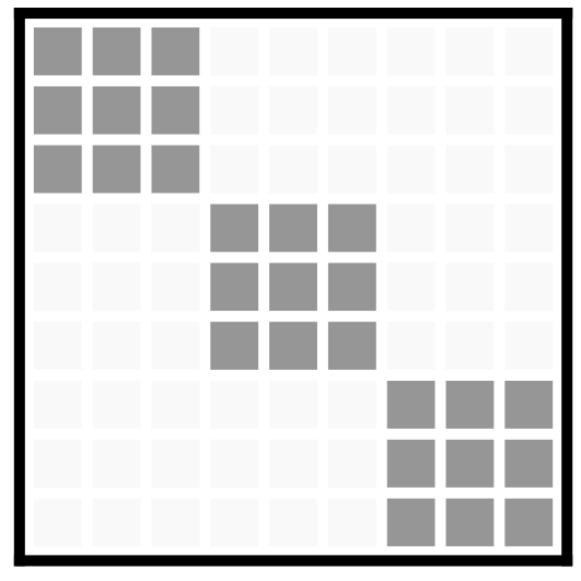
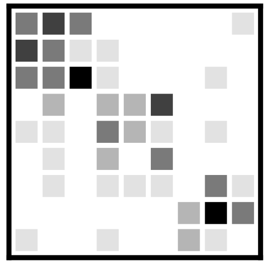
We use the stochastic block model Holland et al. 1983 as the generator. First, we divide two sets of vertices $(U,V)$ into $m$ communities, $\{(U_{1},V_{1}),(U_{2},V_{2}),\cdots,(U_{m},V_{m})\}$ , each with $2n$ vertices and $|U_{i}|=|V_{i}|=n,\forall i\in\{1,2,\cdots,m\}$ . We generate $G=\left<U,V,E\right>$ with the probability of edge $(u,v)$ to be

p(u,v)\propto\begin{cases}1&$u,v$\text{ are in the same community},\\ \alpha&\text{otherwise},\end{cases}

where $\alpha\in[0,1]$ is a hyper-parameter. See Figure 2 for an example. The sum of probability over all edges is normalized to $1$ so that the probability matrix $\mathbf{P}$ can be regarded as a joint probability distribution between two random variables $X$ and $Y$ with $\Pr[X=u,Y=v]=p(u,v)$ .

Refer to caption — Figure 2: Stochastic block model. We set the number of communities $m=3$ , the size of each community $n=3$ and $\alpha=0.1$ . The left matrix represents the underlying probability distribution and the right one is the frequency matrix of a realization.

4.2 Community Contraction

$f$ -Modularity inherits the three properties of $f$ -mutual information in Lemma 3.9, symmetry, non-negativity and information monotonicity. The first two are obviously guaranteed by the definition of $f$ -modularity, i.e.

•

$\mathbf{Mod}^{f}(\left<U,V,E\right>)=\mathbf{Mod}^{f}(\left<V,U,E\right>)$ ,
•

$\mathbf{Mod}^{f}(\left<U,V,E\right>)\geq 0$ .

However, the last one, non-negativity, may not look straightforward.

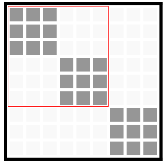
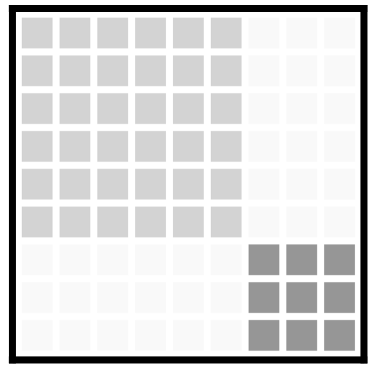
Here we use community contraction to verity that $f$ -modularity is approximately monotone regarding the level of community structure (see Figure 3). The information monotonicity of $f$ -mutual information states that $\textsc{MI}^{f}(T(X);Y)\leq\textsc{MI}^{f}(X;Y)$ where $T(\cdot)\in\mathbb{R}^{|\Sigma_{X}|\times|\Sigma_{X}|}$ is a possibly random operator on $X$ whose randomness is independent of $Y$ . Remark that any operator $T$ essentially multiplies a transition matrix to the joint distribution matrix. From the perspective of network, if we reduce the level of community structure by multiplying a transition matrix to the graph distribution, $f$ -modularity should decrease. We choose community contraction as this operator for ease of presentation.

In detail, we contract two communities $(U_{1},V_{1}),(U_{2},V_{2})$ by allocating the probability evenly within the merged community, i.e., for all $u\in U_{1}\cup U_{2},v\in V_{1}\cup V_{2}$ , we set the new probability of the edge $(u,v)$ to be

p^{\prime}(u,v)=\frac{\sum_{s\in U_{1}\cup U_{2},t\in V_{1}\cup V_{2}}p(s,t)}{|U_{1}\cup U_{2}||V_{1}\cup V_{2}|}.

4.3 Results

Our model assumes the real network is a realization of the underlying distribution with noise. Detecting communities is essentially a process of eliminating noise and recover the true distribution. For example in Figure 2, we aim to “see” the left matrix from the right matrix. So in addition to information monotonicity, we will also show the robustness of $f$ -modularity for estimating the $f$ -mutual information of the true joint distribution. While the theoretical value of mutual information use the true distribution matrix, we set our baseline estimator such that it directly calculates the mutual information by the noisy frequency matrix.

Figure 4 shows our numerical experiments on Jensen Shannon-modularity. We can see

•

Non-negativity: Jensen-Shannon modularity is non-negative and approximately vanishes when the graph has no community structure;
•

Information Monotonicity: when we contract communities, Jensen-Shannon modularity decreases;
•

Robustness: Compared to the baseline, Jensen-Shannon modularity provides a much more robust estimation for the theoretical value of Jensen-Shannon mutual information.

More results for other instances of $f$ -modularity are deferred to the appendix due to the limit of space. The above observations are also fit for them.

5 Conclusion

In this paper, we propose a generalized modularity, $f$ -modularity, based on the dual form of $f$ -mutual information. We find a special case of TVD-modularity exactly matches Newman’s modularity. We also give an algorithm that estimates $f$ -modularity under the case of smooth functions $f$ and low-rank constraints $C$ . Finally, we validate the properties of $f$ -modularity by numerical experiments. Our work not only develops new measures for community structure, but also provides an information-theoretical interpretation to the concept of modularity. Modularity and mutual information, though lying in different areas, are two sides of the same coin.

So far we mainly focused on the low-rank constraint in this work for its simplicity. Our future work will explore not only better rank selection algorithms but also different constraints. Another interesting direction is to study networks with different topologies, like nested networks. We would like to employ information-theoretical tools to quantify more features in networks other than modularity.

References

Ali and Silvey [1966] Syed Mumtaz Ali and Samuel D Silvey. A general class of coefficients of divergence of one distribution from another. Journal of the Royal Statistical Society: Series B (Methodological), 28(1):131–142, 1966.
Brandes et al. [2007] Ulrik Brandes, Daniel Delling, Marco Gaertler, Robert Gorke, Martin Hoefer, Zoran Nikoloski, and Dorothea Wagner. On modularity clustering. IEEE transactions on knowledge and data engineering, 20(2):172–188, 2007.
Chang et al. [2018] Zhenhai Chang, Hui-Min Cheng, Chao Yan, Xianjun Yin, and Zhong-Yuan Zhang. On approximate equivalence of modularity, d and non-negative matrix factorization. arXiv preprint arXiv:1801.03618, 2018.
Cherifi et al. [2019] Hocine Cherifi, Gergely Palla, Boleslaw K Szymanski, and Xiaoyan Lu. On community structure in complex networks: challenges and opportunities. Applied Network Science, 4(1):1–35, 2019.
Cover [1999] Thomas M Cover. Elements of information theory. John Wiley & Sons, 1999.
Danon et al. [2005] Leon Danon, Albert Diaz-Guilera, Jordi Duch, and Alex Arenas. Comparing community structure identification. Journal of statistical mechanics: Theory and experiment, 2005(09):P09008, 2005.
Fortunato [2010] Santo Fortunato. Community detection in graphs. Physics reports, 486(3-5):75–174, 2010.
Girvan and Newman [2002] Michelle Girvan and Mark EJ Newman. Community structure in social and biological networks. Proceedings of the national academy of sciences, 99(12):7821–7826, 2002.
Golub and Reinsch [1971] Gene H Golub and Christian Reinsch. Singular value decomposition and least squares solutions. In Linear algebra, pages 134–151. Springer, 1971.
Haq et al. [2019] Nandinee Fariah Haq, Mehdi Moradi, and Z Jane Wang. Community structure detection from networks with weighted modularity. Pattern Recognition Letters, 122:14–22, 2019.
Holland et al. [1983] Paul W Holland, Kathryn Blackmond Laskey, and Samuel Leinhardt. Stochastic blockmodels: First steps. Social networks, 5(2):109–137, 1983.
Kong and Schoenebeck [2019] Yuqing Kong and Grant Schoenebeck. An information theoretic framework for designing information elicitation mechanisms that reward truth-telling. ACM Transactions on Economics and Computation (TEAC), 7(1):1–33, 2019.
Lee and Seung [1999] Daniel D Lee and H Sebastian Seung. Learning the parts of objects by non-negative matrix factorization. Nature, 401(6755):788–791, 1999.
Malliaros and Vazirgiannis [2013] Fragkiskos D Malliaros and Michalis Vazirgiannis. Clustering and community detection in directed networks: A survey. Physics reports, 533(4):95–142, 2013.
Masuda et al. [2017] Naoki Masuda, Mason A Porter, and Renaud Lambiotte. Random walks and diffusion on networks. Physics reports, 716:1–58, 2017.
Muff et al. [2005] Stefanie Muff, Francesco Rao, and Amedeo Caflisch. Local modularity measure for network clusterizations. Physical Review E, 72(5):056107, 2005.
Newman and Girvan [2004] Mark EJ Newman and Michelle Girvan. Finding and evaluating community structure in networks. Physical review E, 69(2):026113, 2004.
Newman [2004] Mark EJ Newman. Fast algorithm for detecting community structure in networks. Physical review E, 69(6):066133, 2004.
Newman [2006a] Mark EJ Newman. Finding community structure in networks using the eigenvectors of matrices. Physical review E, 74(3):036104, 2006.
Newman [2006b] Mark EJ Newman. Modularity and community structure in networks. Proceedings of the national academy of sciences, 103(23):8577–8582, 2006.
Newman [2016] Mark EJ Newman. Equivalence between modularity optimization and maximum likelihood methods for community detection. Physical Review E, 94(5):052315, 2016.
Nguyen et al. [2010] XuanLong Nguyen, Martin J Wainwright, and Michael I Jordan. Estimating divergence functionals and the likelihood ratio by convex risk minimization. IEEE Transactions on Information Theory, 56(11):5847–5861, 2010.
Porter et al. [2009] Mason A Porter, Jukka-Pekka Onnela, and Peter J Mucha. Communities in networks. Notices of the AMS, 56(9):1082–1097, 2009.
Rockafellar and others [1966] R Tyrrell Rockafellar et al. Extension of fenchel’duality theorem for convex functions. Duke mathematical journal, 33(1):81–89, 1966.
Srebro and Jaakkola [2003] Nathan Srebro and Tommi Jaakkola. Weighted low-rank approximations. In Proceedings of the 20th International Conference on Machine Learning (ICML-03), pages 720–727, 2003.
Veldt et al. [2018] Nate Veldt, David F Gleich, and Anthony Wirth. A correlation clustering framework for community detection. In Proceedings of the 2018 World Wide Web Conference, pages 439–448, 2018.
Young et al. [2018] Jean-Gabriel Young, Guillaume St-Onge, Patrick Desrosiers, and Louis J Dubé. Universality of the stochastic block model. Physical Review E, 98(3):032309, 2018.
Zhang and Moore [2014] Pan Zhang and Cristopher Moore. Scalable detection of statistically significant communities and hierarchies, using message passing for modularity. Proceedings of the National Academy of Sciences, 111(51):18144–18149, 2014.

Appendix A Experimental Results on Jensen-Shannon Modularity

(a)

\alpha

=0.1

(b)

\alpha

=0.2

(c)

\alpha

=0.3

(d)

\alpha

=0.4

(e)

\alpha

=0.5

(f)

\alpha

=0.6

Figure 5: Jensen-Shannon Modularity under Community Contraction. The settings are the same as in Figure 4.

Appendix B Experimental Results on KL-Modularity

(a)

\alpha

=0.1

(b)

\alpha

=0.2

(c)

\alpha

=0.3

(d)

\alpha

=0.4

(e)

\alpha

=0.5

(f)

\alpha

=0.6

Figure 6: KL-Modularity under Community Contraction. The corresponding KL-mutual information is Shannon mutual information. Other settings are the same as in Figure 4.

Appendix C Experimental Results on Pearson-Modularity

(a)

\alpha

=0.1

(b)

\alpha

=0.2

(c)

\alpha

=0.3

(d)

\alpha

=0.4

(e)

\alpha

=0.5

(f)

\alpha

=0.6

Figure 7: Pearson-Modularity under Community Contraction. As Pearson-divergence does not require the non-negativity of

D_{u,v}

, we can use SVD for the low-rank approximation. Other settings are the same as in Figure 4.

Modularity and Mutual Information in Networks: Two Sides of the Same Coin

Abstract

1 Introduction

2 Related Work

3 ff-Modularity

3.1 Frequency Matrix and Random Matrix

Definition 3.1 (Frequency Matrix 𝐅\mathbf{F}).

Example 3.2 (Seller-Buyer).

Definition 3.3 (Random Matrix 𝐉\mathbf{J}).

Lemma 3.4.

Proof of Lemma 3.4.

3.2 ff-Divergence and ff-Mutual Information

Definition 3.5 (ff-Divergence Ali and Silvey 1966).

Definition 3.6 (Fenchel Duality Rockafellar and others 1966).

Lemma 3.7 (Dual Form of ff-DivergenceNguyen et al. 2010).

Definition 3.8 (ff-Mutual Information Kong and Schoenebeck 2019).

Lemma 3.9 (Properties of ff-Mutual Information Kong and Schoenebeck 2019).

3.3 ff-Modularity

Definition 3.10 (ff-Modularity).

Instances of ff-Modularity.

Example 3.11 (TVD-Modularity).

Example 3.12 (KL-Modularity).

Example 3.13 (Pearson-Modularity).

Newman’s modularity ≈\approx TVD-Modularity.

Optimization for smooth functions.

4 Numerical Experiments

4.1 Data Generation

4.2 Community Contraction

4.3 Results

5 Conclusion

References

Appendix A Experimental Results on Jensen-Shannon Modularity

Appendix B Experimental Results on KL-Modularity

Appendix C Experimental Results on Pearson-Modularity

3 $f$ -Modularity

Definition 3.1 (Frequency Matrix $\mathbf{F}$ ).

Definition 3.3 (Random Matrix $\mathbf{J}$ ).

3.2 $f$ -Divergence and $f$ -Mutual Information

Definition 3.5 ( $f$ -Divergence Ali and Silvey 1966).

Lemma 3.7 (Dual Form of $f$ -DivergenceNguyen et al. 2010).

Definition 3.8 ( $f$ -Mutual Information Kong and Schoenebeck 2019).

Lemma 3.9 (Properties of $f$ -Mutual Information Kong and Schoenebeck 2019).

3.3 $f$ -Modularity

Definition 3.10 ( $f$ -Modularity).

Instances of $f$ -Modularity.

Newman’s modularity $\approx$ TVD-Modularity.