Probing the Solar Meridional Circulation using Fourier Legendre Decomposition
Abstract
We apply the helioseismic methodology of Legendre Function Decomposition to 88 months of Dopplergrams obtained by the Helioseismic and Magnetic Imager (HMI) as the basis of inferring the depth variation of the mean meridional flow, as averaged between 20 and 60 degrees latitude and in time, in both the northern and southern hemispheres. We develop and apply control procedures designed to assess and remove center-to-limb artifacts, using measurements obtained by performing the analysis with respect to artificial poles at the east and west limbs. Forward modeling is carried out, using sensitivity functions proportional to the mode kinetic energy density, to evaluate the consistency of the corrected frequency shifts with models of the depth variation of the meridional circulation in the top half of the convection zone. The results, taken at face value, imply substantial differences between the meridional circulation in the northern and southern hemisphere. The inferred presence of a return (equator-ward propagating) flow at a depth of approximately 40 Mm below the photosphere in the northern hemisphere is surprising and appears to be inconsistent with many other helioseismic analyses. This discrepancy may be the result of an inadequacy of our methodology to remove systematic errors in HMI data. Our results appear to be at least qualitative similar to those by Gizon et al. (2020) which point to an anomaly in HMI data that is not present in MDI or GONG data.
I Introduction
Meridional circulation is a crucial, but poorly constrained, component of magnetic flux transport and dynamo models (Choudhuri et al. 1995; Wang et al. 1991; Wang et al. 2002; Dikpati & Gilman 2006; Dikpati & Gilman 2007, e.g.). In many types of flux-transport models, for example, it plays an important role in determining the period or amplitude of the solar cycle (Hathaway et al. 2003; Upton & Hathaway 2014, e.g.). In Babcock-Leighton type dynamo models, the meridional circulation provides the “conveyor belt” that submerges the surface poloidal field of a given solar cycle deep into the convection zone to be sheared by differential rotation and advected towards the equator by the meridional return flow (Charbonneau 2010, e.g.). The meridional flow is also an important dynamical element in theoretical and numerical models of solar and stellar differential rotation and convection (Glatzmaier & Gilman 1982; Brun & Toomre 2002; Rempel 2005; Miesch 2007, e.g.).
Measurements of the surface manifestation of meridional circulation have typically indicated poleward flows between 10 and 20 m s-1 (LaBonte & Howard 1982; Topka et al. 1982; Hathaway et al. 1996; Schou 2003; Rightmire-Upton et al. 2012, e.g.). Meridional circulation is difficult to measure accurately, since its amplitude is considerably smaller than, say, solar rotation. Helioseismic analyses of the subsurface properties of this flow are particularly challenging. The frequencies of global modes are insensitive to first order to the meridional circulation, unlike the rotational splitting which has facilitated the successful determination of the subsurface properties of rotation (Brown et al. 1989; Schou et al. 1998, e.g.). However, meridional flows have been measured and modeled with a variety of local seismic methods. Many studies have mostly focused on the meridional circulation near the surface (e.g. within a few tens of Mm below the surface), where the sensitivity of helioseismic measurements to flows is highest (González Hernández et al. 1999; Haber et al. 2002; Hughes & Thompson 2003; Zhao & Kosovichev 2004; González Hernández et al. 2008; Komm et al. 2015a; Komm et al. 2015b; Komm et al. 2018, e.g.).
Probing the deeper properties of the meridional circulation is difficult due, in large part, to expected low signal-to-noise values of the measurements (Braun & Birch 2008) and the presence of systematic artifacts (Duvall & Hanasoge 2009; Zhao et al. 2012, e.g.). Nonetheless, numerous studies involving measurements and inferences of the deeper properties of the meridional flow have been carried out (Giles et al. 1997; Braun & Fan 1998; Chou & Ladenkov 2005; Mitra-Kraev & Thompson 2007; Schad et al. 2013; Woodard et al. 2013; Zhao et al. 2013; Kholikov & Hill 2014; Kholikov et al. 2014; Liang & Chou 2015; Rajaguru & Antia 2015; Liang et al. 2018; Gizon et al. 2020, e.g.). The last decade in particular has seen a renewal of interest in probing the deep meridional circulation, making use of the long duration datasets provided by the ground-based Global Oscillation Network Group (GONG) instruments (Harvey et al. 1996; Harvey et al. 1998) and the Helioseismic and Magnetic Imager (HMI) instrument (Scherrer et al. 2012; Schou et al. 2012) onboard the Solar Dynamics Observatory (SDO) spacecraft (Pesnell et al. 2012). However, there is not yet a consensus on the general structure and properties of the meridional circulation, especially in the deeper two-thirds of the convection zone.
The purpose of this study is to perform a follow-up to the meridional-flow measurements carried out by Braun & Fan 1998. In that study, we applied the method now known as Fourier Legendre decomposition (hereafter FLD) to one month of GONG data and 8 days of Dopplergrams from the Michelson Doppler Imager (MDI) instrument (Scherrer et al. 1995) onboard the Solar and Heliospheric Observatory. With various modifications, the FLD method has been employed in a number of subsequent studies of solar meridional circulation (Krieger et al. 2007; Doerr et al. 2010) as well as undergone development and validation studies (Roth et al. 2016; Hecht & Roth 2018). We note that the method used by Mitra-Kraev & Thompson 2007 is closely related to FLD analysis, but applied selectively to waves propagating along the central meridian. Novel aspects of the present work include: the development of procedures to assess and remove the center-to-limb artifact, the application of FLD to a long duration (7.3 years) of HMI Dopplergrams, a comparison and assessment of different ridge-peak finding methods, and an assessment of the sensitivity of the measurements to azimuthal order. We apply an updated version of the forward modeling approach employed by Braun & Fan 1998 in order to infer the latitude-averaged meridional flow, for each hemisphere, in the top half of the convection zone.
II Data Analysis
II.1 Fourier Legendre Decomposition
The basic concept of FLD is similar to ring-diagram analysis (Hill 1988), and infers subsurface flows by measuring and modeling the Doppler distortion in the power spectra. Compared to most ring-diagram methods, the FLD technique is optimized for the detection of meridional flows by properly accounting for spherical geometry and using combinations of Legendre functions of the first and second kind to characterize poleward or equatorward propagating waves. The basis for the technique is the expansion of the observed Dopplergram signal , a function of colatitude , azimuthal angle and time , into traveling wave components:
| (1) |
where is the temporal frequency, is the degree, and is the azimuthal order. and are the complex amplitudes of poleward and equatorward waves respectively. is a normalized function,
| (2) |
where and are Legendre functions of the first and second kind respectively and is a normalization factor. The expansion of waves in terms of propagating functions has been utilized for many decades in nuclear and quantum physics (Nussenzveig 1965; Fuller 1975, e.g.) where the operation is called “nearside-farside decomposition.” In helioseismology, the first application of this expansion was carried out by Bogdan et al. 1993 as an extension to spherical coordinates of Fourier Hankel decomposition (Braun et al. 1987; Braun et al. 1988, e.g.), and used to measure the absorption and scattering of modes by sunspots.
The functions are orthogonal such that
| (3) |
over the annular domain , where is the Kronecker delta function. As Bogdan et al. 1993 note, the condition described by equation (3) generally requires non-integer values of . For practical purposes, such as the ability to compute Legendre functions using recursion relations (Press et al. 1992), a restriction to integer values of degree renders equation (3) approximately true for a subset of equally spaced . Furthermore, the orthogonality condition restricts the range of azimuthal order for each degree , such that
| (4) |
Physically, this condition selects waves which propagate at least to the highest latitudes in the annular domain. The normalization function
| (5) |
where . The choice of and under the constraint of equation (3) restricts the independence of the coefficients and to degrees separated by
| (6) |
The operations needed to estimate the coefficients and are
| (7) |
and
| (8) |
where is the spatial window function and is the duration of the time interval as determined from observational constraints.
For the measurement of meridional circulation, the pole is placed at either the north or south pole of the Sun, and the resulting distortion between power spectra of poleward ( and equatorward ( propagating waves is typically characterized as a “frequency shift” (at fixed degree and azimuthal order) of the relevant or -mode peak. For short-lived “local” modes, with typically high degrees or high frequencies, and for which peaks in power spectra are blended into continuous ridges in the domain, this frequency shift can be readily identified as a shifting of the ridge position. Longer-lived “global” modes, typically at low degrees and low frequencies, show isolated peaks, whose frequencies are not affected to first order by meridional flow (Gough & Hindman 2010). The “frequency shifts” which can be measured in this mode regime through FLD methods result from a redistribution of power, through mode coupling produced by advection, between modes of nearby degree and which leak into the observed spectra (Roth et al. 2016). Our determination of frequency shifts is discussed further in §III.
II.2 Observations and Initial Analysis
We use full-disk Dopplergrams, taken with a temporal cadence of once per 45 seconds, obtained from the HMI instrument onboard the Solar Dynamics Observatory over an 88 month interval spanning 2010 June through 2017 September. Initial processing of the HMI full-disk Dopplergrams include removal of the line-of-sight component of solar rotation using a fit to a plane function. The residual is divided by the cosine of the heliocentric angle to account for the (primarily) radially oscillating waves. To avoid foreshortening and other effects of the extreme limb, we mask out the data beyond a heliocentric angle of 60∘. A remapping of the line-of-sight Doppler signal to spherical coordinates is performed using bi-linear interpolation. The coordinate grid has a spacing of in both latitude and longitude, which is close to the HMI pixel size at disk center and oversamples the image elsewhere. The range of latitudes considered in our analysis is between 20∘ and 60∘ in the northern hemisphere and -60∘ to -20∘ in the southern hemisphere. At the surface, this latitude range comfortably straddles the peak of the meridional circulation as directly inferred in the photosphere (Hathaway & Rightmire 2010, e.g.). This latitude range excludes many, but not all, active regions. No masking of active regions (Liang & Chou 2015, e.g.) was performed and we note there is no consensus on the use of this operation.
II.3 Center-to-Limb Artifacts and Control Measurements
One of the first manifestations of artifacts, or systematic effects in local helioseismology mistakenly identified as flows, appear to be the high-latitude “counter cells,” of opposite direction from the poleward flows inferred at lower latitudes (Haber et al. 2002). These features were demonstrated to be of spurious origin by González Hernández et al. 2006. More generalized large-scale artifacts (hereafter “pseudo flows”) which vary with distance from disk center have subsequently been detected (Braun & Birch 2008; Duvall & Hanasoge 2009; Zhao et al. 2012; Greer et al. 2013; Kholikov et al. 2014; Chen & Zhao 2017; Chen & Zhao 2018, e.g.). As noted by Duvall & Hanasoge 2009, light from the limb of the Sun will arrive 2.3 seconds after that emitted from disk center. This has the consequence of decreasing the observed travel time of waves propagating from the limb toward disk center while increasing the times for waves propagating in the opposite direction. This should give rise to an apparent radially symmetric pseudo flow directed towards disk center. It has been suggested (Baldner & Schou 2012; Zhao et al. 2012) that spatial asymmetries between upward and downward convective motions can cause pseudo flows of either direction (towards disk center or the limb) and which depend on heliocentric angle and choice of observable (e.g. Dopplergram or continuum intensity) or instrument.
Pseudo flows have been observed with a variety of helioseismic methods, including holography (Braun & Birch 2008), time-distance helioseismology (Duvall & Hanasoge 2009; Zhao et al. 2012; Rajaguru & Antia 2015; Chen & Zhao 2017; Chen & Zhao 2018, e.g.), and ring-diagram analysis (Greer et al. 2013, e.g.). From studies such as these, it appears that pseudo flows exhibit complex variations (including sign changes) with disk position, instrumentation, and mode properties including both frequency and wavenumber. Rajaguru & Antia 2020 suggest that the inference of the deep meridional circulation using time-distance analyses may vary significantly with the choice of temporal frequency of the pseudo-flow measurements. This may help to explain discrepancies in inferences obtained from different groups using the same datasets.
A starting point to correct the data is the assumption that the pseudo flows are symmetric about the Sun-observer axis. For the case of travel-time differences inferred using time-distance methods, a method first suggested by Duvall & Hanasoge 2009, and subsequently carried out by others (Zhao et al. 2012; Kholikov et al. 2014, e.g.) involves subtracting the travel-time differences, measured along the axis connecting the east and west limbs, from the measured north-south differences along the central meridian.
In this work, we apply a analogous procedure suitable for the FLD method. Specifically, a set of control analyses are performed with the geometry rotated 90∘ from the true north (or south) poles to analogous locations at the east and west limbs (Figure 1). So that the annular regions covered by these control measurements sample a similar, but rotated, spatial distribution of pixels at all times, the positions of the poles of these analyses (hereafter referred to as “pseudo-poles”) should mirror the yearly oscillation of the true poles towards or away from the observer. As discussed further in §III.1, control analyses at both east and west limbs are necessary to separate the effects of the pseudo flow from those due to solar rotation. Furthermore, since we are interested in analyzing the meridional flows in both hemispheres, we require a pair of control analyses specifically designed for each hemisphere, as illustrated in Figure 1. If the positions of the pseudo poles were not tracked to follow solar rotation, the solar photosphere would rotate substantially across the annular regions in the control analyses over any reasonable analysis time frame. The rotational signal introduced would be up to two orders of magnitude greater than the desired pseudo-flow signals and the resulting distortion of the power spectra would be detrimental to the analysis. Rotating the positions of the pseudo poles at a mean Carrington rate alleviates most of this distortion, while leaving a smaller effect due to deviations of solar differential rotation from the Carrington rate. The cost of this procedure is the requirement to limit the duration of the analyses such that the geometry does not substantially change over the chosen time span. All of these considerations suggest a strategy whereby control measurements are made over short intervals while the position of the pseudo poles is tracked at the Carrington rate and reset back to its initial position on the solar disk at the start of each interval. Figure 1 illustrates the change in the annular regions over 8 hours, which is the interval chosen for this analysis.


We use the term “nominal” to indicate the measurements used to infer the meridional flow in the northern and southern hemisphere and distinguish them from the “control” measurements described above. For the nominal measurements, which use coordinates aligned with the north and south poles, we remap from Dopplergram coordinates to Carrington coordinates, thereby applying the same tracking. Unlike the control measurements we are free to consider longer time intervals for the nominal measurements without unwelcome distortions of the power spectra due to rotation. For this study, we consider power spectra constructed over time intervals of 8 hours (as in the control measurements) as well as over one month intervals. This allows an assessment of potential issues arising from the 8-hr limitation of the control measurements. For the “one-month” power spectra, we extract and pad data from each calendar-month with zeros as necessary to compute spectra over a fixed duration of 31.0 days. The nominal measurements are obtained over the full 88 month duration, while the control measurements were carried out using the first 24 months of the time interval. Prior assessments of the pseudo flow (Liang et al. 2018, see their Figure 4) suggest that this systematic effect changes little with time.
The symmetry between the east and west control measurements allow the contribution of solar differential rotation to be assessed and removed from the center-to-limb aligned pseudo flow since the former has opposite effects between the two measurements while the latter has the same sense in both measurements. This is analogous to the pseudo-flow assessment used in some time-distance analyses designed to extract the antisymmetric component of the east-to-west travel-time shifts within a narrow equatorial strip (Zhao et al. 2013). Our control measurements are by design not confined to the equatorial regions, but instead require an identical, but rotated, annulus which includes relatively high-latitude contributions (see, for example, the control annuli in red shown in Figure 1). Unfortunately, this results in a small but significant component of the true meridional flow leaking (equally) into both control measurements in a fashion which is non-trivial to separate from the pseudo flows. To see this, we use the terms “outward” and “inward” to describe the directional sensitivity of the control measurements in analogy to the “equatorward” and “poleward” directions in the nominal measurements. The leakage of meridional flows into the control measurements results from the fact that, away from disk center, meridional lines connecting the nominal north and south poles are not perpendicular to the meridional lines connecting the pseudo poles at the east and west limbs. Consequently, a fraction of the poleward directed flow in either hemisphere leaks into the control annuli as an outward directed flow with respect to either (east or west) pseudo pole. Alternately, an equatorward flow from either (true) pole produces an inward directed leakage in the control measurements. We estimate the magnitude of this leakage (which is on the order of 20%) and discuss its mitigation in §III.2.
II.4 Power Spectra
The coefficients and are computed from equations (7) and (8) using numerical integration over azimuthal angle and colatitude and the use of fast Fourier transforms (specifically, the FFTW library) in time. The window function is determined from the latitude ranges and 60∘ limb cutoff illustrated in Figure 1 within which the data is apodized with a Welch window in and a raised cosine bell, with a width of 12∘, in . We compute coefficients for degrees and azimuthal orders , except for modes with degree for which the highest order is determined from equation (4). The contribution from low frequencies is reduced by taking successive differences in time of the relevant integrand for each and . Potentially compromised Dopplergrams (e.g. due to cosmic rays or other issues) are identified from an examination of the variation in time (over each 8-hour or 31-day interval) of the sum over and of the squared values. Anomalous values of this parameter, defined as less than one-half of, or greater than twice, the median over the interval, identify problematic Dopplergrams which are then removed from the time series through substitution with zeros. Over the 88-month interval, only about 6.6% of HMI Dopplergrams were either rejected through this criteria or otherwise missing from the time series.
Power spectra for poleward () and equatorward () traveling waves are summed over azimuthal order:
| (9) | |||
| (10) |
where and the floor function is the greatest integer less than or equal its argument. This summation is justified since the sensitivity of the frequency shifts is very nearly independent of , as discussed further in §IV. Spectra for each 8-hr or 31-day interval are then summed over time. The nominal measurements are summed over the entire 88-month duration and also over one-year intervals for each calendar year 2011 through 2016. The latter are used to estimate errors in the frequency shift measurements (§III), and to examine the temporal variation of the shifts (§V). Figure 2 shows power spectra for poleward traveling waves over the northern hemisphere and averaged over the 88-month duration, as determined over 8-hr and 31-day intervals. It is difficult to ascertain differences between the two spectra when displayed as images with similar scales and dimensions, so line plots of the spectra of selected degrees are directly compared in Figure 3.


To extract the frequency shifts for inferring the meridional circulation we have chosen to use the 8-hr power spectra. This ensures that the shifts are determined uniformly for both the nominal and control measurements, the latter requiring the primary limitation on the temporal duration as described earlier. The comparison of the spectra between 8-hr and 31-day intervals is instructive, however. For modes with degree greater than about 150, there is little difference in the appearance of the mode ridges other than the difference in the frequency sampling. This can be seen in the top panel of Figure 3 for example. As one examines the spectra at successively lower , it becomes apparent that global peaks are resolved in the 31-day spectra but not in the 8-hr spectra. These multiple narrow peaks represent modes with nearby which leak into the power spectra due to the window function which isolates a 40∘ strip in latitude). Distinct, if blended, ridges corresponding to different radial orders are visible in the 8-hr spectra above the red line in Figure 2, which corresponds to constant phase speed mHz. This phase speed corresponds to a lower turning point depth of 100 Mm, or about midway in the convection zone. The middle panel of Figure 3 shows an example of the power spectra in this regime. Below the red line in Figure 2 it is clear that distinct ridges for each order are not resolved (e.g. bottom panel of Figure 3). This is due to the overlap of the leaked modes between neighboring radial orders which is more readily observed in the 31-day spectra.
II.5 Multi-Ridge Fitting
To extract the frequency shifts between poleward and equatorward traveling waves from the power spectra (as well as the inward and outward traveling waves in the control spectra) we compared three different methods. These included 1) determining the difference between the centroid frequencies of poleward and equatorward ridges (Braun & Fan 1998, e.g. as carried out by), 2) finding the peak in the cross-correlation function between the two ridges, and 3) fitting the power spectra to models which account for the shape of the ridges and their shifts in frequency. Comparison of the different methods as well as tests with artificial power spectra are described in Appendix A. These tests demonstrated the presence of systematic biases in the first two methods above which are due to the contamination from ridges with neighboring radial orders. Methods which simultaneously fit multiple ridges can account for the blending of nearby ridges in a manner not possible with those which fit isolated ridges (Greer et al. 2014, e.g.).
To carry out multi-ridge fitting (hereafter “MRF”), we first extract the power at each as a function of frequency. Using lookup tables of mode frequencies we identify the number of ridges, , with differing radial order present below 5 mHz. We then fit the power to a sum of Gaussians, with free parameters of amplitude, width, and central frequency, and a background term consisting of a cubic polynomial. The frequency shift of interest is
| (11) |
where and are the central Gaussian frequencies from the fits to spectra and respectively for the ridge of degree and radial order . The fitting code employs MPFIT routines (Markwardt 2009) which carry out a non-linear least-squares fit with uniform weighting. Fits using a weighting by the inverse of the square of the error, as determined from year-to-year fluctuations in the spectra, were also attempted. These fits generally underestimated the peak values and were judged inferior to fits using uniform weighting. Fits to Lorentzian functions were also attempted, but these tended to greatly overestimate the troughs between the ridge peaks and forced a negative background term. This suggests that the Lorentzian functions have line wings which are too large compared to the observed spectra. Initial guesses for the Gaussian parameters were obtained from fitting individual Gaussian functions to isolated ridges for each radial order. Constraints on the fits include 1) keeping the Gaussian amplitudes and widths positive and 2) keeping the central frequencies within a window spanning the mid-points to adjacent radial orders. Figure 4 shows an example of our modeling result for degree . In some instances, ridges at high temporal frequency could not be fit satisfactorily. An example of this failure is illustrated by the ridge in Figure 4.

The blue curve shows the residuals (observations minus fit) with the same error bars as observed in the power spectra. The residuals and its error bars have been multiplied by a factor of 5 for clarity.
III Frequency Shifts
The frequency shift in equation (11) denotes the difference between the central ridge frequency of the poleward (or inward) traveling waves minus that of the equatorward (or outward) traveling waves. It is convenient (particularly in regards to the modeling efforts described in §IV) to define a scaled frequency shift :
| (12) |
where is the solar radius. The units of are that of speed (e.g. m s-1) and has a physical meaning as the equivalent uniform (i.e. “solid-body”) angular rotational speed of a shell of a star needed to yield a given frequency shift of waves fully confined within the shell. In the application here, it is useful to think of this hypothetical shell as roughly spanning the solar surface to the depth of the lower turning point of a given mode . Inferring the actual radius (depth) dependence of the flow from the collection of measurements is discussed in §IV but, at least for modes with shallow turning points (e.g. large ), provides an estimate of the local flow speed as experienced by those waves. The sign of the frequency shift is such that a positive value of indicates a flow (or pseudo flow) which is directed poleward (or inward).
Errors in the determination of were obtained by dividing the 88-month dataset into yearly intervals and defining the errors to be the year-to-year root-mean-squared fluctuations in the frequency shifts divided by the square-root of the total time interval in years. In general, the errors at phase speeds below about 0.015 mHz are of order 1 m s-1, but increase sharply with increasing phase speed to nearly 10 m s-1. A common mode set, consisting of nominal measurements with an error less than 10 m s-1 for both hemispheres, was established. This mode set spanned a range in degree , frequencies between 2.0 and 5.0 mHz, and radial orders from to 12. Among the 565 modes in the final dataset, the deepest penetrating modes have phase speeds around 0.04 mHz and lower turning point depths around 100 Mm below the surface.
III.1 Control Measurements
Figure 5 shows the scaled frequency shifts for the east and west control analyses which were designed to mirror the (rotated) position of the latitude annulus to correct the northern-hemisphere measurements. We refer to these east and west control measurements as and respectively. Results for the control analyses designed for the southern hemisphere (not shown) are similar. For phase speeds below 0.02 mHz, and have opposite sign and exhibit linear trends with phase shift which have slopes of opposite sign. The sign of these shifts is indicative of a net eastward directed flow, which is retrograde with respect to solar rotation, and can be identified as the residual effects of differential rotation relative to the tracked Carrington rate. At phase speeds above 0.02 mHz, the results for both control measurements show positive shifts approaching nearly 50 m s-1.

Adding the frequency shifts for the east and west control measurements cancels out the effects of rotation such that the remaining shifts are primarily caused by the center-to-limb effect. However, an alternative way of achieving this is to sum the relevant inward or outward power spectra over both control measurements and extracting the frequency shifts, , from the resulting combined spectra. This method results in incrementally less noise than frequency-shift subtraction and was employed here. Figure 6 shows plotted as functions of phase speed (upper panel) and mode frequency (lower panel). Results for the two control measurements designed for the southern hemisphere (not shown) are similar. The pseudo flow revealed by these measurements contains both outward and inward directed components. As the phase speed of the modes increase, the pseudo flow increases from inward directed with amplitudes around -2 m s-1 to outward directed with amplitudes reaching up to 50 m s-1 for the deepest modes. Viewed as a function of frequency, each radial order shows pseudo flows which decrease and become inflows with increasing frequency. Many of the radial orders converge to a common function of frequency above 4.5 mHz. A remarkably similar result for the frequency and phase-speed variation of the center-to-limb effect was found by Greer et al. 2013 using ring-diagram analysis of HMI data with 30∘ tiles. The frequency variation of the center-to-limb effect has also been explored using a Fourier analysis of time-distance correlations (Chen & Zhao 2018). Our results are at least qualitatively similar to these results which include a change of sign of the pseudo flow near 5 mHz.

III.2 Corrected Frequency Shifts
Figure 7 shows the nominal frequency-shift measurements for the northern hemisphere before and after a correction for the center-to-limb effect. The shallowest modes show raw frequency shifts of around 15 m s-1, which can be identified with the meridional flow. However, the entirety of the measurements resemble those obtained from the control measurements (the top panel of Figure 6) but offset vertically. Subtracting the latter from the raw measurements removes most of the center-to-limb effect, but this operation alone fails to account for the leakage of the true meridional flow signal into the control measurements as discussed at the end of §II.3.

To appropriately include this effect in our correction, we assume the control measurements and contain a component due to leakage which is proportional by a factor to the signal produced by the meridional circulation in the nominal measurements. As discussed in Appendix B this suggests a modified operation to retrieve the desired shifts due to meridional circulation, , from the raw shifts :
| (13) |
We assume which is estimated from an evaluation of surface measurements of the meridional circulation and the assumption that the leakage does not vary with phase speed among the mode set. This estimate is discussed and justified in Appendix B. Consequences of a deviation of from this constant value on our derived meridional flow profiles are discussed in §VI. The bottom panel of Figure 7 shows the results of our correction for the northern hemisphere (similar results for the southern hemisphere are not shown) and represent the frequency shifts we consider in our forward modeling efforts.
IV Forward Modeling
The goal of the modeling is to infer the depth variation of the latitude-averaged meridional flow
| (14) |
in each hemisphere. The flow is related to the frequency shifts , with the subscript or omitted but understood, as
| (15) |
where the kernels represent the kinetic energy density (Gough & Toomre 1983; Birch et al. 2007) and have been used in prior FLD modeling (Braun & Fan 1998; Roth et al. 2016). The function describes the sensitivity of the shifts with azimuthal order (see Appendix C) while the angular brackets around the ratio represent an average over the same azimuthal orders used to sum the power spectra from which the scaled shifts were extracted. Figure 8 shows some examples of the kernels .

We employ a “forward modeling” approach whereby the observed frequency shifts are directly compared with results obtained from equation (15) using different choices of the flow . We first average the measurements in narrow bins in phase speed to obtain the mean and its standard error. The bins are chosen to isolate groups of twenty frequency-shift measurements. Figure 9 shows the averaged values, with error bars given by the standard error of the mean. The averaging reveals systematic differences between the two hemispheres. At phase speeds below 0.01 mHz, the corrected shifts in the northern hemisphere exceed those in the south by an amount just under 1 m s-1. At a phase speed near 0.01 mHz the shifts for both hemispheres are in agreement, but at higher phase speeds the shifts in the northern hemisphere are significantly smaller than in the south with the difference increasing with phase speed. At a phase speed near 0.03 mHz, the results differ by about 4 m s-1 with the results in the south being roughly twice that in the north. The biggest difference between hemispheres occurs at the highest phase-speed bin, where the northern shift is of opposite sign than those in the south.

For each hemisphere, two flow profiles were obtained by trial and error. The goal is that the two flow functions represent plausible fits to the upper and lower limits of the mean shifts as determined by their standard errors. In general, the predicted scaled shifts corresponding to the 565 observed modes for a given flow lie with very little scatter around a relatively smooth and continuous function of phase speed (Figure 10). This facilitates a rapid assessment of a candidate flow through visual inspection of plots such as Figure 10.

We use a characterization of the flow which consists of a cubic spline interpolation between three prescribed anchor points spanning depths between 0.5 Mm above the photosphere and approximately 25 Mm below the photosphere (this lower depth varied somewhat among the four fits). The speed at the three anchor points was determined through trial and error and involved fixing the shallowest points first and adjusting successively deeper values until suitable matches between observed and predicted frequency shifts were obtained. Below the deepest anchor point the flow function was assumed for simplicity to contain of a sum of exponential and linear terms. The flow speed at the deepest anchor point fixes the amplitude of the exponential term while the linear term is set to zero at this depth. There are consequently two free parameters (the decay scale of the exponential and the slope of the linear term) which determine the depth dependence of the flow below this depth. Figure 11 shows the final four flows, from which the predicted shifts shown in Figure 10 were obtained. For the results in the northern hemisphere, the (negative) bin-averaged shift at the highest phase speed in Figure 10 was ignored, as no reasonable flow model considered could reproduce this apparently anomalous measurement. The model flows shown in Figure 11 are similar between hemispheres over the shallow regime over which the flows were characterized by cubic splines. However significant differences are observed below 25 Mm, with the most surprising result being the onset of a relatively shallow equatorward return flow in the northern hemisphere at around 40 Mm. Results for the southern hemisphere are consistent with a decrease in speed with depth, but remain poleward over the depths considered.

V Temporal Variations
To further explore the apparent hemispheric differences in the frequency shifts illustrated in Figure 9, we compare the variation of this difference with hemispheric differences in solar activity. As discussed in §II.4, errors were estimated from frequency shifts assessed from power spectra averaged over yearly intervals for each calendar year. These year-to-year measurements also allow their temporal variations to be determined. To clearly see general trends while maintaining some discrimination with mode depth, the shifts are averaged over mode sets corresponding to three ranges in phase-speed. We establish three sets, such that the phase speed ranges from 0 to 0.01 mHz in the “shallow” set, 0.01 to 0.02 mHz in the “intermediate” set, and 0.02 to 0.04 mHz in the “deep” set. We note the year-to-year frequency shifts are not corrected for either the center-to-limb effect or the leakage, which does not effect the relative temporal changes we are interested in examining.
Figure 12 shows the results of this averaging, which is done for both hemispheres, along with the monthly smoothed sunspot numbers (SILSO World Data Center 2021, hereafter SSN;). The shallow and intermediate mode-averaged shifts, for both hemispheres, show gradual increases above the errors over the six years examined, while the shifts deepest set remain constant within the errors. This variation is plausibly related to solar-cycle changes in the meridional circulation in this cycle (Zhao et al. 2014, e.g.). Of particular relevance is that the hemispheric differences which were found in the total 88 month set are present for most, if not all, of the period shown. The tendency for the shallow mode shifts in the north to exceed those in the south, is observed for most of the interval, although this difference nearly disappears for the last two years. On the other hand, the north-south discrepancy in the deepest mode shifts is notably present with similar magnitude (roughly two seconds) during all six years. During the same interval, solar cycle 24 was initially dominated by a distinct peak of sunspot numbers in the northern hemisphere, followed over two years later by a peak in sunspot number in the south. This would argue against the hemispheric differences in the frequency-shift measurements being related in a simple way to asymmetries in the distribution of magnetic regions.

VI Discussion
Taken at face value the results as illustrated by Figures 10 and 11 are unexpected in that the shallow return flow present in the north hemisphere appear to be inconsistent with most prior determinations of the meridional circulation which employ multi-year observations and which attempt to remove the effects of center-to-limb related artifacts. Specifically, most analyses involving modeling time-distance travel-time perturbations show a poleward flow in both hemispheres which persist from the surface down to approximately 0.9 (i.e. about 70 Mm below the surface). This includes the analyses of Zhao et al. 2013; Jackiewicz et al. 2015; Rajaguru & Antia 2015; Chen & Zhao 2017 A notable exception is the recent analysis of Gizon et al. 2020 which is discussed below. In general, uncertainties in the inference of the flow increase with the depth of those inferences. This makes the discrepancy with other helioseismic analyses at a relatively shallow depth all the more puzzling. If we assume that the results for at least the northern hemisphere are spurious, than the challenge is to understand the cause of what appears to be an uncorrected artifact. Of course, real hemispheric differences in the meridional circulation may very well exist, but it is worth considering the possible nature of pseudo-flows which are themselves asymmetric.
The comparison of the time variation of the frequency shifts with the sunspot numbers for both hemispheres (Figure 12) indicates that the observed hemispheric differences in the 88-month interval persist regardless of the level of solar activity or its preference to one hemisphere over the other. While this doesn’t rule out the presence of real solar-cycle variations in flows (Chou & Dai 2001; Zhao & Kosovichev 2004; González Hernández et al. 2008; Hathaway & Rightmire 2010, e.g.), or potential pseudo-flow artifacts related to magnetic regions (Liang & Chou 2015, e.g.), there is no direct correlation between hemispheric differences in solar activity and the differences in the frequency shifts.
Errors in the control measurements due to uncertainties of the leakage discussed in Appendix B appear to be too small to account for the hemispheric differences observed in Figure 9. In particular we note that likely errors in the leakage factor amounting to 20% of the selected value of 0.84 (see Appendix B) cause uncertainties in the deepest scaled frequency shifts of around 1 m s-1. These are smaller than the standard errors of the observations shown in Figure 9 and substantially smaller than the 4 m s-1 discrepancy observed at the highest phase speeds.
It is plausible that the results may be compromised by incorrect assumptions regarding the azimuthal invariance of the center-to-limb correction. At the deepest phase speeds, the frequency shifts due to the pseudo flow shown in the top panel of Figure 6 have amplitudes that exceed by about a factor of ten the expected shifts due to meridional circulation in the nominal measurements (bottom panel of Figure 7). Thus, relative differences between the pseudo-flow at either true pole and the east and west limbs amounting to only 5-10% could produce 50-100% uncertainties in the corrected shifts, and is sufficient to account for an anomalous hemispheric difference consistent with observations.
Of particular relevance is the recent analysis of Gizon et al. 2020 which compared inferences of the meridional circulation obtained from three data sources (MDI, GONG, and HMI). While they generally found the results obtained from MDI and GONG were consistent with a single circulation cell in both hemispheres, with a return flow present at 0.8 (approximately 140 Mm below the surface), they also found systematic errors unique to the measurements using HMI data. Specifically this consisted of significantly shorter north-south travel-time differences in the northern hemisphere than the southern hemisphere which appears at least qualitatively similar to the hemispheric differences between FLD frequency shifts presented here. Our results therefore provide some qualified confirmation of this HMI-specific anomaly, while not directly addressing differences between the results of Gizon et al. 2020 and other HMI-based analyses (Zhao et al. 2013; Rajaguru & Antia 2015; Chen & Zhao 2017, e.g.). Understanding the source of this anomaly is critical and, to this end, employing FLD methods with GONG and/or MDI observations would be highly useful.
In addition to the need to resolve this HMI-based mystery, other improvements to the FLD technique as applied to the study of the meridional circulation seem warranted. Probably the most important is extending the method to model the low- global-mode spectra required to infer flows in the bottom half of the convection zone. As discussed in §II.4 the issue at hand is the blending of power ridges of adjacent radial order. It is clear from the results shown here that employing time intervals of 8-hr duration for the analysis is not sufficient to resolve the relevant low- power spectra (e.g. Figure 3). Longer duration spectra are readily obtainable for the nominal measurements, but this is not the case for the control observations for which shorter duration intervals were required to minimize rotation effects. Consequently, extending the FLD analysis deeper may require novel methods of correcting the frequency shifts for center-to-limb artifacts.
Appendix A Ridge-peak Finding Comparisons
We tested different peak-finding methods to extract the frequency shifts shown in §III. In addition to the multi-ridge fitting (MRF) method described in §III, we test two other methods. First, we employed the centroid method used by Braun & Fan 1998, whereby the frequency shift between poleward and equatorward traveling waves is
| (A1) |
where is a frequency window surrounding a ridge with degree and radial order . The other method involves the cross-correlation function evaluated between and :
| (A2) |
where the frequency shift between poleward and equatorward traveling waves is given by the value of which maximizes . Typically, the frequency shift is small compared to the spacing in frequency over which the cross-correlation function is computed discretely. Consequently, it is necessary to model and interpolate the peak of the cross-correlation function in some fashion. The main free parameters in these methods include the choice of the individual frequency windows and, for the cross-correlation method, the means by which peak in the correlation is identified. Estimation and removal of simple “background” power may be carried out as well. For example, Braun & Fan 1998 inferred and subtracted a simple linear term between high and low frequencies, in an admittedly ad-hoc fashion, before measuring the centroid frequencies.
In addition to comparing the results obtained using different methods applied to the observed poleward and equatorward power spectra, we also tested each method using artificial power spectra. Specifically, to make these tests relevant to the applications at hand, we use the fits of the MRF method (§III), without noise, as spectra to test the centroid (hereafter referred to as CENT) and cross-correlation (hereafter XCORR) methods. Not surprisingly, the MRF method applied to these noiseless spectra return the expected input parameters to high precision. Tests on the artificial spectra were made with and without the cubic background term.
The results of these comparisons and tests are shown in Figures 13 and 14. Undeniably the most disappointing results from these tests are that both the centroid and cross-correlation methods show significant systematic differences from the MRF results in a manner which is readily reproduced with the noiseless artificial spectra. For example, the centroid method consistently underestimates the shifts relative to MRF applied to solar spectra (Figure 13) and likewise underestimates the true shifts in the artificial spectra. The similarly between the left and right panels in this figure is a reflection of how well the artificial spectra capture the relevant properties of the actual solar power spectra in these tests. Of particular note is the systematic bias which increases in magnitude with increasing phase speed. The cause of this is contamination of power from nearby ridges which becomes worse as the frequency spacing between ridges decreases with higher phase speed. Systematic differences at lower phase speed (i.e. less than 0.02 mHz) are also observed and, in the case of the artificial spectra, are identified as contamination from the cubic background term in those spectra. The interpretation of this background is uncertain in the context of the solar spectra and may result from either an actual contribution of low-frequency convective signal or an inadequacy of the MRF method to describe the properties of the mode spectra (for example, a failure of Gaussian functions to reproduce the wings of the ridges). Whatever its meaning, it is clear that its presence adds to the contamination problem experienced at higher phase speeds due to the narrow ridge separation. Unfortunately, tests with different frequency windows, e.g. making them narrower than the default values which span the midpoints to neighboring ridges, produced little or no change in the bias.


Figure 14 shows the results obtained using the cross-correlation method. These results were obtained by fitting the five points bracketing the observed maximum in to the sum of coaligned quadratic and quartic functions:
| (A3) |
where is the desired frequency shift, and , and are constants. Some improvement over the centroid method is apparent in Figure 14 at lower phase speeds, although systematics still exist. At higher phase speeds we observe rapidly increasing differences (left panel) and departures from true values (right panel) in the artificial spectra. Improvements (i.e. approaching zero) are observed at lower phase speeds in the right panel when the background terms are removed, as was the case with the centroid method. Changes in the choice of frequency windows or fitting function (e.g. using Gaussian functions instead of equation [A3]) produced little or no improvement in the general results shown in Figure 14.
In conclusion, we find that the systematic discrepancies encountered with the centroid and cross-correlation methods render them useless in preference to methods (such as MRF) which can explicitly account for the presence and potential contamination of neighboring ridges and possible background (convective) power.
Appendix B Leakage of Meridional Flow into the Control Measurements
We consider the control measurements and and how to include effects of leakage of the meridional flow signal in our center-to-limb correction. We assume that the control shifts consist of components due to the center-to-limb pseudo flow, which we designate , and components due to leakage. We assume the latter is proportional by a factor to the signal produced by the meridional circulation in the nominal measurements. Therefore we have
| (B1) |
where are the expected nominal frequency shifts due to meridional circulation alone. This are related to the raw shifts via a subtraction of the true center-to-limb shifts:
| (B2) |
Eliminating from equations (B1) and (B2) yields a modified correction operation:
| (B3) |
We expect from a consideration of geometry (as discussed in §II.3) that the leakage is of opposite sign than the nominal meridional flow shifts () so the raw difference overestimates the desired shifts and is corrected by a multiplication by a “leakage factor” which is less than one.
| flow | ||
|---|---|---|
| SF | -0.19 | 0.84 |
| obs (N) | ||
| obs (S) | ||
| a | -0.28 | 0.78 |
| b | -0.26 | 0.79 |
| c | -0.24 | 0.81 |
| d | -0.19 | 0.84 |
| e | -0.17 | 0.85 |
| f | -0.17 | 0.85 |
To constrain the leakage factor, we first consider the shallowest modes (i.e. small phase speeds) and estimate the leakage caused by surface values of the meridional flows. For this purpose, we acquired latitudinal profiles (Upton, private communication) of the surface meridional flows averaged over each Carrington rotation over our 88-month interval and determined from feature tracking (Hathaway & Rightmire 2010; Rightmire-Upton et al. 2012). The profiles take the form of coefficients to polynomial fits to the flow up to fifth order in . For each profile, we perform a coordinate transformation on the vector flow field as viewed in the nominal coordinate system (aligned to the rotation axis) to determine its “inward/outward” component in the coordinate system aligned to the pseudo poles used in the control measurements. The leakage ratio is then given by the spatial average of this component over the observed window function divided by the average of the north/south component in the original coordinate system over the same window. Over the relevant time frame, we obtain the mean and standard deviations of as well as the factor . These values, labeled as flow “SF,” are listed in the first line of Table 1.
Prior observations have suggested that the center-to-limb pseudo flow trends towards zero amplitude as the phase speed (or equivalently, skip-distance in time-distance measurements) decreases (Greer et al. 2013; Chen & Zhao 2017, e.g.). Our own observations (e.g. Figure 6) uniquely show negative values of the control shifts and for the and modes at the smallest phase speeds which plausibly arise to the leakage discussed here. Under the assumption that approaches zero for the shallowest modes, we assess the ratio of and , as averaged over phase speeds mHz. These values, as listed in Table 1 and labeled “obs (N)” and “obs (S)” respectively. represent upper limits to , thus allowing some small positive center-to-limb contribution . but are consistent with the expectation from the surface flows “SF.”
The remaining task is to estimate the leakage expected for the deeper measurements. It is tempting to consider the possibility that the leakage is invariant (or at least sufficiently so) over our range of frequency-shift measurements, which enables us to multiply all shifts with a simple constant in the correction (B3). To this end, it is worth considering what conditions might produce large variations in the leakage with depth. It is clear from the geometry of the control measurements that the range in sampled by the control annulus extends to the equator, unlike the nominal measurements which are cut off for . Thus, a redistribution of the flow in latitude with increasing depth needs to be considered. Using the same coordinate transformation and integration described above, We compute the variation of the factor among different toy models of the dependence. Some assumptions which help to constrain possible profiles include: (1) the meridional circulation remains nearly antisymmetric about the equator, and (2) its variation with latitude is smooth and maintains the same sign (poleward or equatorward) over each hemisphere. Using the simple functions illustrated in Figure 15 we obtain the results listed in Table 1. We note that a flow given by a multiplication of the functions shown in Figure 15 by a constant with either sign will produce the same leakage. Thus, these results are relevant equally for poleward and equatorward (e.g. return) flows. The smallest (largest) values of the leakage factor occur when the relative contributions of the flow are concentrated more at the lower (higher) latitudes. However, variations of the leakage parameter remain comfortably modest over all of the cases considered.
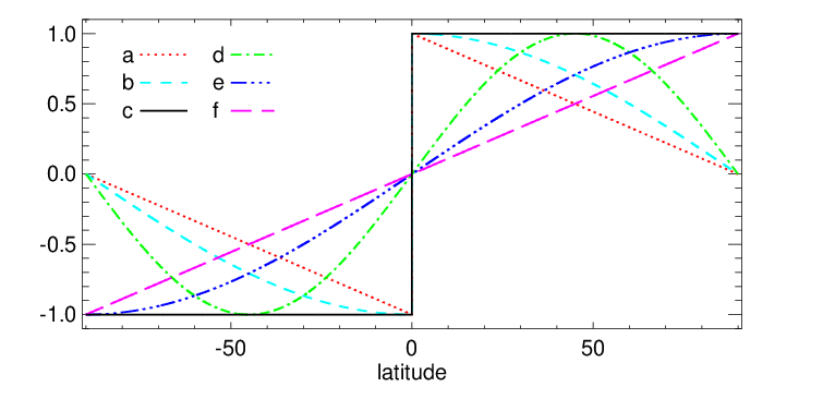
On the basis of these results, we assume for our inferences here that the leakage factor has a nominal value of 0.84. However, in evaluating the results inferred in §IV, we consider the possibility that this factor varies with mode depth within a conservative range of 0.75 to 0.90, which represents a net uncertainty of about 20%.
Appendix C Sensitivity Functions
The sensitivity of the frequency shift to an interior flow , which is steady over the time interval of the analysis and smooth in and , can be derived by a perturbation analysis of the wave equation in the presence of the flow (Gough & Toomre 1983). In spherical coordinates, one obtains:
| (C1) |
where is the density, and and are related to the components of the eigenmodes
| (C2) |
“” distinguishes between poleward and equatorward traveling wave modes, and is the component of the flow in the meridional direction . We can rewrite equation (C1) in terms of the scaled frequency shift :
| (C3) |
where is the average of the meridional flow component (equation 14), , and the kernel is given by the mode kinetic energy density:
| (C4) |
The function contains the terms on the right hand side of equation (C1) which depend on the azimuthal order :
| (C5) |
and to a good approximation. The ratio gives the sensitivity of the frequency shift to azimuthal order, relative to , and is shown in the left panel of Figure 16. The ratio reduces to a single-valued function of , sometimes referred to as the “impact parameter” in scattering theory, except when this parameter approaches and exceeds the limit imposed by equation (4). The right panel of Figure 16 shows the average of this ratio over the azimuthal orders for which the power spectra were summed in this work. For the modes used in the forward modeling the values of this ratio are between about 0.97 and 1.0. In the modeling (§IV) we compare the frequency shifts from the -summed power spectra with predictions made using equation (C3) with the ratio replaced by the averages shown in the right panel of Figure 16.


References
- Baldner & Schou (2012) Baldner, C. S., & Schou, J. 2012, ApJ, 760, L1
- Birch et al. (2007) Birch, A. C., Gizon, L., Hindman, B. W., & Haber, D. A. 2007, ApJ, 662, 730
- Bogdan et al. (1993) Bogdan, T. J., Brown, T. M., Lites, B. W., & Thomas, J. H. 1993, ApJ, 406, 723
- Braun & Birch (2008) Braun, D. C., & Birch, A. C. 2008, Sol. Phys., 251, 267
- Braun et al. (1987) Braun, D. C., Duvall, Jr., T. L., & LaBonte, B. J. 1987, ApJ, 319, L27
- Braun et al. (1988) —. 1988, ApJ, 335, 1015
- Braun & Fan (1998) Braun, D. C., & Fan, Y. 1998, ApJ, 508, L105
- Brown et al. (1989) Brown, T. M., Christensen-Dalsgaard, J., Dziembowski, W. A., et al. 1989, ApJ, 343, 526
- Brun & Toomre (2002) Brun, A. S., & Toomre, J. 2002, ApJ, 570, 865
- Charbonneau (2010) Charbonneau, P. 2010, Liv Rev Solar Phys, 7, doi:10.12942/lrsp-2010-3
- Chen & Zhao (2017) Chen, R., & Zhao, J. 2017, ApJ, 849, 144
- Chen & Zhao (2018) —. 2018, ApJ, 853, 161
- Chou & Dai (2001) Chou, D.-Y., & Dai, D.-C. 2001, ApJ, 559, L175
- Chou & Ladenkov (2005) Chou, D.-Y., & Ladenkov, O. 2005, ApJ, 630, 1206
- Choudhuri et al. (1995) Choudhuri, A. R., Schussler, M., & Dikpati, M. 1995, A&A, 303, L29
- Dikpati & Gilman (2006) Dikpati, M., & Gilman, P. A. 2006, ApJ, 649, 498
- Dikpati & Gilman (2007) —. 2007, Sol. Phys., 241, 1
- Doerr et al. (2010) Doerr, H.-P., Roth, M., Zaatri, A., Krieger, L., & Thompson, M. J. 2010, Astronom. Nach., 331, 911
- Duvall & Hanasoge (2009) Duvall, Jr., T. L., & Hanasoge, S. M. 2009, in Astronomical Society of the Pacific Conference Series, Vol. 416, Solar-Stellar Dynamos as Revealed by Helio- and Asteroseismology: GONG 2008/SOHO 21, ed. M. Dikpati, T. Arentoft, I. González Hernández, C. Lindsey, & F. Hill, 103–109
- Fuller (1975) Fuller, R. C. 1975, Phys. Rev. C, 12, 1561
- Giles et al. (1997) Giles, P. M., Duvall, Jr., T. L., Scherrer, P. H., & Bogart, R. S. 1997, Nature, 390, 52
- Gizon et al. (2020) Gizon, L., Cameron, R. H., Pourabdian, M., et al. 2020, Science, 368, 1469
- Glatzmaier & Gilman (1982) Glatzmaier, G. A., & Gilman, P. A. 1982, ApJ, 256, 316
- González Hernández et al. (2008) González Hernández, I., Kholikov, S., Hill, F., Howe, R., & Komm, R. 2008, Sol. Phys., 252, 235
- González Hernández et al. (2006) González Hernández, I., Komm, R., Hill, F., et al. 2006, ApJ, 638, 576
- González Hernández et al. (1999) González Hernández, I., Patrón, J., Bogart, R. S., & The SOI Ring Diagram Team. 1999, ApJ, 510, L153
- Gough & Hindman (2010) Gough, D., & Hindman, B. W. 2010, ApJ, 714, 960
- Gough & Toomre (1983) Gough, D. O., & Toomre, J. 1983, Sol. Phys., 82, 401
- Greer et al. (2013) Greer, B., Hindman, B., & Toomre, J. 2013, in Fifty Years of Seismology of the Sun and Stars, ed. K. Jain, S. C. Tripathy, F. Hill, J. W. Leibacher, & A. A. Pevtsov, Vol. 478 (San Francisco: Astron. Soc. Pacific), 199–204
- Greer et al. (2014) Greer, B. J., Hindman, B. W., & Toomre, J. 2014, Sol. Phys., 289, 2823
- Haber et al. (2002) Haber, D. A., Hindman, B. W., Toomre, J., et al. 2002, 570, 855
- Harvey et al. (1998) Harvey, J., Tucker, R., & Britanik, L. 1998, in ESA Special Publication, Vol. 418, Structure and Dynamics of the Interior of the Sun and Sun-like Stars, ed. S. Korzennik, 209
- Harvey et al. (1996) Harvey, J. W., Hill, F., Hubbard, R. P., et al. 1996, Science, 272, 1284
- Hathaway et al. (2003) Hathaway, D. H., Nandy, D., Wilson, R. M., & Reichmann, E. J. 2003, ApJ, 589, 665
- Hathaway & Rightmire (2010) Hathaway, D. H., & Rightmire, L. 2010, Science, 327, 1350
- Hathaway et al. (1996) Hathaway, D. H., Gilman, P. A., Harvey, J. W., et al. 1996, Science, 272, 1306
- Hecht & Roth (2018) Hecht, E., & Roth, M. 2018, ApJ, 862, 145
- Hill (1988) Hill, F. 1988, ApJ, 333, 996
- Hughes & Thompson (2003) Hughes, S. J., & Thompson, M. J. 2003, in GONG+ 2002. Local and Global Helioseismology: the Present and Future, ed. H. Sawaya-Lacoste, Vol. 517 (Noordwijk: ESA), 307–310
- Jackiewicz et al. (2015) Jackiewicz, J., Serebryanskiy, A., & Kholikov, S. 2015, ApJ, 805, 133
- Kholikov & Hill (2014) Kholikov, S., & Hill, F. 2014, Sol. Phys., 289, 1077
- Kholikov et al. (2014) Kholikov, S., Serebryanskiy, A., & Jackiewicz, J. 2014, ApJ, 784, 145
- Komm et al. (2015a) Komm, R., González Hernández, I., Howe, R., & Hill, F. 2015a, Sol. Phys., 290, 1081
- Komm et al. (2015b) —. 2015b, Sol. Phys., 290, 3113
- Komm et al. (2018) Komm, R., Howe, R., & Hill, F. 2018, Sol. Phys., 293, 145
- Krieger et al. (2007) Krieger, L., Roth, M., & von der Lühe, O. 2007, Astronom. Nach., 328, 252
- LaBonte & Howard (1982) LaBonte, B. J., & Howard, R. 1982, Sol. Phys., 80, 361
- Liang & Chou (2015) Liang, Z.-C., & Chou, D.-Y. 2015, ApJ, 805, 165
- Liang et al. (2018) Liang, Z.-C., Gizon, L., Birch, A. C., Duvall, T. L., & Rajaguru, S. P. 2018, A&A, 619, A99
- Markwardt (2009) Markwardt, C. B. 2009, in Astronomical Data Analysis Software and Systems XVIII, ed. D. A. Bohlender, D. Durand, & P. Dowler, Vol. 411 (San Francisco: Astron. Soc. Pacific), 251
- Miesch (2007) Miesch, M. S. 2007, Astronom. Nach., 328, 998
- Mitra-Kraev & Thompson (2007) Mitra-Kraev, U., & Thompson, M. J. 2007, Astronom. Nach., 328, 1009
- Nussenzveig (1965) Nussenzveig, H. M. 1965, Annals of Physics, 34, 23
- Pesnell et al. (2012) Pesnell, W. D., Thompson, B. J., & Chamberlin, P. C. 2012, Sol. Phys., 275, 3
- Press et al. (1992) Press, W. H., Teukolsky, S. A., Vetterling, W. T., & Flannery, B. P. 1992, Numerical Recipes in C. The Art of Scientific Computing, 2nd Ed. (Cambridge University Press)
- Rajaguru & Antia (2015) Rajaguru, S. P., & Antia, H. M. 2015, ApJ, 813, 114
- Rajaguru & Antia (2020) —. 2020, Astrophysics and Space Science Proceedings, 57, 107
- Rempel (2005) Rempel, M. 2005, ApJ, 622, 1320
- Rightmire-Upton et al. (2012) Rightmire-Upton, L., Hathaway, D. H., & Kosak, K. 2012, ApJ, 761, L14
- Roth et al. (2016) Roth, M., Doerr, H. P., & Hartlep, T. 2016, A&A, 592, A106
- Schad et al. (2013) Schad, A., Timmer, J., & Roth, M. 2013, ApJ, 778, L38
- Scherrer et al. (1995) Scherrer, P. H., Bogart, R. S., Bush, R. I., et al. 1995, Sol. Phys., 162, 129
- Scherrer et al. (2012) Scherrer, P. H., Schou, J., Bush, R. I., et al. 2012, Sol. Phys., 275, 207
- Schou (2003) Schou, J. 2003, ApJ, 596, L259
- Schou et al. (1998) Schou, J., Antia, H. M., Basu, S., et al. 1998, ApJ, 505, 390
- Schou et al. (2012) Schou, J., Scherrer, P. H., Bush, R. I., et al. 2012, Sol. Phys., 275, 229
- SILSO World Data Center (2021) SILSO World Data Center. 2021, International Sunspot Number Monthly Bulletin and online catalogue
- Topka et al. (1982) Topka, K., Moore, R., LaBonte, B. J., & Howard, R. 1982, Sol. Phys., 79, 231
- Upton & Hathaway (2014) Upton, L., & Hathaway, D. H. 2014, ApJ, 792, 142
- Wang et al. (2002) Wang, Y.-M., Sheeley, Jr., N. R., & Lean, J. 2002, ApJ, 580, 1188
- Wang et al. (1991) Wang, Y.-M., Sheeley, Jr., N. R., & Nash, A. G. 1991, ApJ, 383, 431
- Woodard et al. (2013) Woodard, M., Schou, J., Birch, A. C., & Larson, T. P. 2013, Sol. Phys., 287, 129
- Zhao et al. (2013) Zhao, J., Bogart, R. S., Kosovichev, A. G., Duvall, Jr., T. L., & Hartlep, T. 2013, ApJ, 774, L29
- Zhao & Kosovichev (2004) Zhao, J., & Kosovichev, A. G. 2004, ApJ, 603, 776
- Zhao et al. (2014) Zhao, J., Kosovichev, A. G., & Bogart, R. S. 2014, ApJ, 789, L7
- Zhao et al. (2012) Zhao, J., Nagashima, K., Bogart, R. S., Kosovichev, A. G., & Duvall, Jr., T. L. 2012, ApJ, 749, L5