Minimization of ion micromotion with artificial neural network
Abstract
Minimizing the micromotion of the single trapped ion in a linear Paul trap is a tedious and timing-consuming work, but is of great importance in cooling the ion into the motional ground state as well as maintaining long coherence time, which is crucial for quantum information processing and quantum computation. Here we demonstrate that systematic machine learning based on artificial neural networks can quickly and efficiently find optimal voltage settings for the electrodes using rf-photon correlation technique, consequently minimizing the micromotion to the minimum. Our approach achieves a very high level of control for the ion micromotion, and can be extended to other configurations of Paul trap.
pacs
37.10.Mn, 37.10.Pq, 37.20.+jIntroduction
Recently the wave of artificial intelligence has made great changes to industry, marketing and social life such as facial/voice recognition, prediction of consumer behaviors. Due to its great success, machine learning algorithms have been rapidly applied to diverse research subjects Awad and Khanna 2015, including physics Arsenault et al. 2014; Rupp 2015; Li et al. 2015; Pilania et al. 2016; Carrasquilla and Melko 2017; Raissi and Karniadakis 2018; Radovic et al. 2018; Carleo et al. 2019; Sarma et al. 2019; Schütt et al. 2020, chemistry Goh et al. 2017; Kitchin 2018; Butler et al. 2018; Tkatchenko 2020; Cartwright 2020, biology Tarca et al. 2007; Angermueller et al. 2016; Ching et al. 2018, astronomy Ball and Brunner 2010; Way et al. 2012; VanderPlas et al. 2012; Ivezić et al. 2014; Baron 2019, ecnomics Herbrich et al. 1999; Mullainathan and Spiess 2017; Athey 2018 and finance Bose and Mahapatra 2001; Khandani et al. 2010; Heaton et al. 2017; Klaas 2019, weather forecast Lai et al. 2004; Sharma et al. 2011; Kendon et al. 2014; Choi et al. 2016; Holmstrom et al. 2016, medical science Kononenko 2001, material science Raccuglia et al. 2016; Ward et al. 2016; Ramprasad et al. 2017; Sanchez-Lengeling and Aspuru-Guzik 2018; Schmidt et al. 2019 and drug discovery Deo 2015; Obermeyer and Emanuel 2016; Ching et al. 2018. In physics, it is successful in solving problems ranging from high-energy Radovic et al. 2018 and string theory to condensed matter Arsenault et al. 2014; Pilania et al. 2016; Carrasquilla and Melko 2017, to astrophysics VanderPlas et al. 2012, to atomic, molecular and optical physics Seif et al. 2018; Sarma et al. 2019. Always, it play a significant role in reducing the complexity of the problem and in optimization of one or multiple experimental parameter with various mathematical algorithms. Especially, it can reduce a N-dimensional problem to only a few dimensions, which greatly simplifies the experimental realization of any NP-hard problem in physics, such as improve the fidelity of a quantum gate operation using trapped ions ( ) for quantum computation and quantum information processing. However, it remains an uncharted territory and a mistery to physicists that, to what extend can it assist and boost the research.
In current research, we try to minimize the micromotion of the trapped ion. The excess micromotion of a trapped ion can come from stray electric fields, RF pickup by one of the DC electrodes, and a phase difference between the RF electrodes. It causes the ion to oscillate at the RF frequency, resulting in Doppler shifts as the ion moves towards or away from the laser beam. This will reduce the efficiency of both cooling and state detection, and could heavily reduce the ion’s lifetime. More generally, it deteriorate the harmonic character of the ion motion, making it impossible to construct a ion quantum gate with high fidelity. Therefore, it is important to eliminate the micromotion to the highest degree possible.
Multiple techniques are widely used for minimizing the excess micromotion of trapped ions, such as sideband Chwalla 2009; Doret et al. 2012, parametric excitation Narayanan et al. 2011; Tanaka et al. 2012, photon-correlation Berkeland et al. 1998; Keller et al. 2015 etc. All of them are quite successfully, photon-correlation especially, in terms of reach high-level of minimization of excess micromotion. However, most of these methods requires adjusting DC voltages repeatedly and is quite time-consuming, usually take hours and even days. Since there is no direct mathematical relation between DC voltages and the excess micromotion index , and the minimization of the micromotion is clearly a multi-dimensional problem, which is a natural playground where machine learning plays a major role. Here we apply neural-network-based machine learning to fast solve the problem using photon-correlation technique.
Theoretical Scheme
.0.0.1 Excess Micromotion
The trapping potential of an ion trap can be written as Leibfried et al. 2003
| (1) |
where the first term represents the dynamics confinement in Y-Z radial plane, and the second term represents the static confinement along the X axial direction. and is the amplitude and frequency of the RF oscillating electric field, respectively. is the amplitude of the DC electric field, and is the distance between the potential center and the electrodes in the radial plane. We assume that the principle axes of the radial trapping potential are aligned along the directions and , as shown in Figure 3, and assume the equations of motion along each direction are fully decoupled, we can write the ion’s equation of motion in the form of Mathieu equation Keller et al. 2015
| (2) |
Here is the stray electric field along that effectively push the ion away from the RF null point, causing the RF null and the DC null to be in different positions. and are the charge and mass of the ion, and the and are related to applied voltages. The solution to Eq.2 to lowest order in and is
| (3) |
where is a displacement of the equilibrium position from the rf node due to any residual static electric field, is the secular motion amplitude with the frequency of . is the phase of secular motion determined by the initial conditions of the ion position and velocity. is the phase of the micromotion. The motion corresponding to the term is driven by the applied ac electric field, and is called micromotion. From Eq.3, this micromotion consists of an intrinsic contribution from the periodic displacement due to the secular motion, and an excess micromotion with an amplitude caused by the ac electric field at position .
With the assumption of and , the amplitude of this excess micromotion can be written as Berkeland et al. 1998
| (4) |
where
| (5) |
The excess micromotion can induce the first- and second-order Doppler effect, which will significantly alter the excitation spectrum of an atomic transition. Assuming the electric field of the excitation laser has the amplitude , frequency , phase , and wave vector , then this laser field can be expressed in the rest frame of the ion undergoing excess micromotion:
| (6) | ||||
Applying Fourier transform to Eq.(6), we get Riehle 2006
| (7) | |||
Consequently, the detected fluorescence can be written as Keller et al. 2015
| (8) | ||||
where is the detuning of the excitation laser frequency from the atomic resonance, the phase , and .
.0.0.2 Neural-Network-based Machine Learning
Machine learning algorithms are typically divided into three categories: (1) Supervised Algorithms which uses labeled datasets to train algorithm to construct a model, which can predict new data Mohri et al. 2018; Russell and Norvig 2002. It includes neural network, support vector machine, k-nearest neighbors, decision Tree, random forest, and so on. (2) Unsupervised Algorithms which learn from unlabeled data Hinton et al. 1999. It can divide data into different groups via learning. (3) Reinforcement Algorithms which is about how intelligent agents take action to maxmize the reward Kaelbling et al. 1996. In this paper, we try to solve a object-oriented problem which is minimizing a physical parameter, the micromotion index of a trapped ion, as much as possible, thus we apply first category machine learning algorithm, neural-network-based machine learning to one of the most fundamental researches in quantum mechanics, the motional study of driven harmonic oscillator in mixed external fields.
One of the most successful techniques to attack such a high-dimensional problem is the artificial neural networks (16). They can perform exceedingly well in a variety of scenarios ranging from image and speech recognition (17) to game playing (18). Very recently, applications of neural networks to the study of physical phenomena have been introduced (19–23). Although Applying neural network technique has been used in few cases, it is still of fundamental and practical interest to solve such a high-dimensional problem using neural network based machine learning method. This ability could then be used to minimize ion’s excess micromotion for other types of Paul traps, and to solve other high-dimensional problems that is commonly timing-consuming and hard to address experimentally.
Here we introduce an artificial neural network specified by a set of internal parameters , which represent the input for the machine learning, i.e. the voltages on related compensation electrodes. We present a stochastic framework for reinforcement learning of the parameters , allowing for reaching the optimal minimization of ion’s excess micromotion. The parameters of the neural network are optimized (in other words, trained) by static variational Monte Carlo sampling (24). We validate the accuracy of this approach by measuring the magnitude of the residual excess micromotion right after we apply the learning results (i.e. the output voltages) on the corresponding electrodes. The power of the neural-network based machine learning is demonstrated, obtaining state-of-the-art level of minimization in excess micromotion Berkeland et al. 1998; Keller et al. 2015.
Here we introduce a real-time progressive automatic algorithm to find out the null point of our blade trap. Previous to this work, we find a set of voltages through position compensation, which is ramping up the RF power and keep the ion’s position by adjusting voltages when we ramp down the RF power. Now, we generate a Gaussian distribution of voltage for each compensation electrode using as the center and as the standard deviation. Thus we have a large sets of voltage combination. Then, we apply these voltage sets to the electrodes one at a time, and measure their corresponding photon-correlation spectrum in and direction. Following this, we obtain the micromotion index and for each voltage set by fitting each spectrum to the equation ( ). Based on these voltage sets and their indices, a model can be learned using neural network. Then it can give us a set of voltages which allow for the minimum and rather straightforward using anneal algorithm. Consider the above steps as a cycle/block, we repeat it a number of times, until we find out the actual null point. This is varified by the and .
In our neural network algorithm, we classify these artificial neurons into three class: , , . Each artificial neuron has input and output. For , input is dataset, output is the same of input. For the first , input is the output of , output is data after linear transformation and nonlinear transformation. For the other , input is the output of former , output is also the result of transformation. For , input is the same of output - the output of former .

In Figure 1, we show the basic configuration of an artificial neural network, which include input and , and hidden layer , and output and . The neuron in the hidden layer and the output can be expressed by:
| (9) | ||||
where is activation function. In general, we use rectified linear unit (ReLU) function Nair and Hinton 2010, that is . In this way, we can write down the expression for output neuron with other neurons. After giving all the biases and weights, we can calculate value of all . With input dataset , we now have the prediction by neural network and by measurement. Then we define loss function, also called cost function, or mean squared error (MSE) function
| (10) |
In order to obtain a suitable model to fit the data, we need the loss function as small as possible. Typically, backpropagation (BP) algorithm Goodfellow et al. 2016, combined with stochastic gradient descent (SGD) algorithm Bottou 1998; Kiwiel 2001, is widely used for training artificial neural networks, i.e. to iterate the neural network until the loss function small enough in neural network Orr and Müller 2003.

Figure 2 shows the schematics for the backpropagation algorithm. First, we define the error as the difference between the deduced value from the measurement and the predicted value by the learning machine based on the constructed neural network. Assuming the hidden network has layer with neurons for each layer, the error in would be propagated backwards according to
| (11) |
then the weight will be modified by
| (12) |
So far, we have constructed a BP neural network, in practice, we just need to iterate the BP neural network until the loss function become small enough to get an appropriate model.
Experiment
In this section, we show how to implement the neural network to realize the minimization of the excess micromotion using the machine learning approach. First, we briefly introduce the experimental setup. The ion trap used in this experiment is similar to Johnson et al. 2016. It has four gold-plated ceramic blade electrodes, whose edges are parallel to the longitudinal (x) axis of the trap as shown in Figure 3. Two opposite blades are driven with an RF potential with respect to the other two static blades, creating the transverse (y-z) quadrupole confinement potential. Appropriate static potentials provided by the longitudinal five-segment static blades serve to confine the ion along the x-axis. The RF electric quadrupole potential near the center of the trap is set by the RF amplitude on the trap electrode , and can be closely approximated by . The gap between the electrodes is and in and direction, respectively. The distance from the trap center to the electrodes . Other parameters in our blade trap are: , , , , , , , , , and . With this configuration we achieved trap frequency of with 0.45W RF power.
We measure the photon arrival time as a histogram using RF-photon correlation method, from which excess micromotion index can be obtained by fitting the histrogram profile to equation (1). We supply the machine with the voltages on multiple DC compensation electrodes as the input and the index as the target, then we challenge the machine to discover the hidden high-dimensional voltage-to- surface. This relation between DC voltages and will give us a set of DC voltages, allowing optimal minimization of excess micromotion, which corresponds to the null point in the electric field. Since and in radial direction are strongly coupled together, the smaller , the smaller , only in axial direction and in radial direction instead of all three in three Cartesian coordinates are measured. In the experiment, the detection laser is alternating in and direction for detection of and using photon-correlation technique.


We take a two-input to two-output as an example, where two inputs are voltages on DC2 and DC7 respectively, and two outputs are and respectively. The procedure is carried out with multiple loops until predicted voltage set given by the neural network allow for the desired low level of micromotion. One of the loops is shown in Figure 4. It has two blocks (upper and lower panel) with four steps in each block. First, we generate a series of voltage set in a DC file, with and in the voltage sets having a Gaussian distribution in a large range. The center corresponds to the voltage set by the position compensation Berkeland et al. 1998, which is monitoring the ion position with an EMCCD camera (iXon 897, Andor) at a high RF voltage, then lowering RF voltage and moving ion position to point by adjusting DC voltages. The standard deviation of the distribution are from a roughly estimatation of stable region based on Mathieu equation. After generating the DC file, we send the voltage sets to the electrodes in series through programmable precision DC voltage power supply (BS1-16-14, Stahl-electronics). Then we detect the fluorescence modulation in both x-direction and y-direction by alternately blocking the detection laser in y-direction and x-direction, using a START-STOP time-to-digital converter (HRM-TDC, SensL) to which photon numbers are fed from a photomultiplier tube (H10682-210, Hamamatsu). Each modulation spectra is taken three times to minimize the effects of drifting laser frequency and fluctuating laser power as well as the RF noise.

After this, we deduce the and for each voltage set by fitting Eq.(8) to the measured spectra. Consequently, we use neural network to construct an appropriate model for minimization of excess micromotion. This is followed by the annealing process, which finds out the best voltage set allowing for minimum and simultaneously. Since the range of the voltage sets in first block is relatively large, in order to have a precise voltage set and a better minimization, we repeat the process in the second block, using the voltage set attained from the first block as the center and typically half region of the first block to generate the new distribution of voltage set.
For current learning model, we use 4 hidden layers, each having 100 neurons. The data flow is graphically represented in Figure 4. The output sequence of and from our model is then compared with the measured sequence and over the whole parameter space to evaluate the loss function. Once the loss function reach a value which is smaller than the threshold , we conclude the model is appropriate.


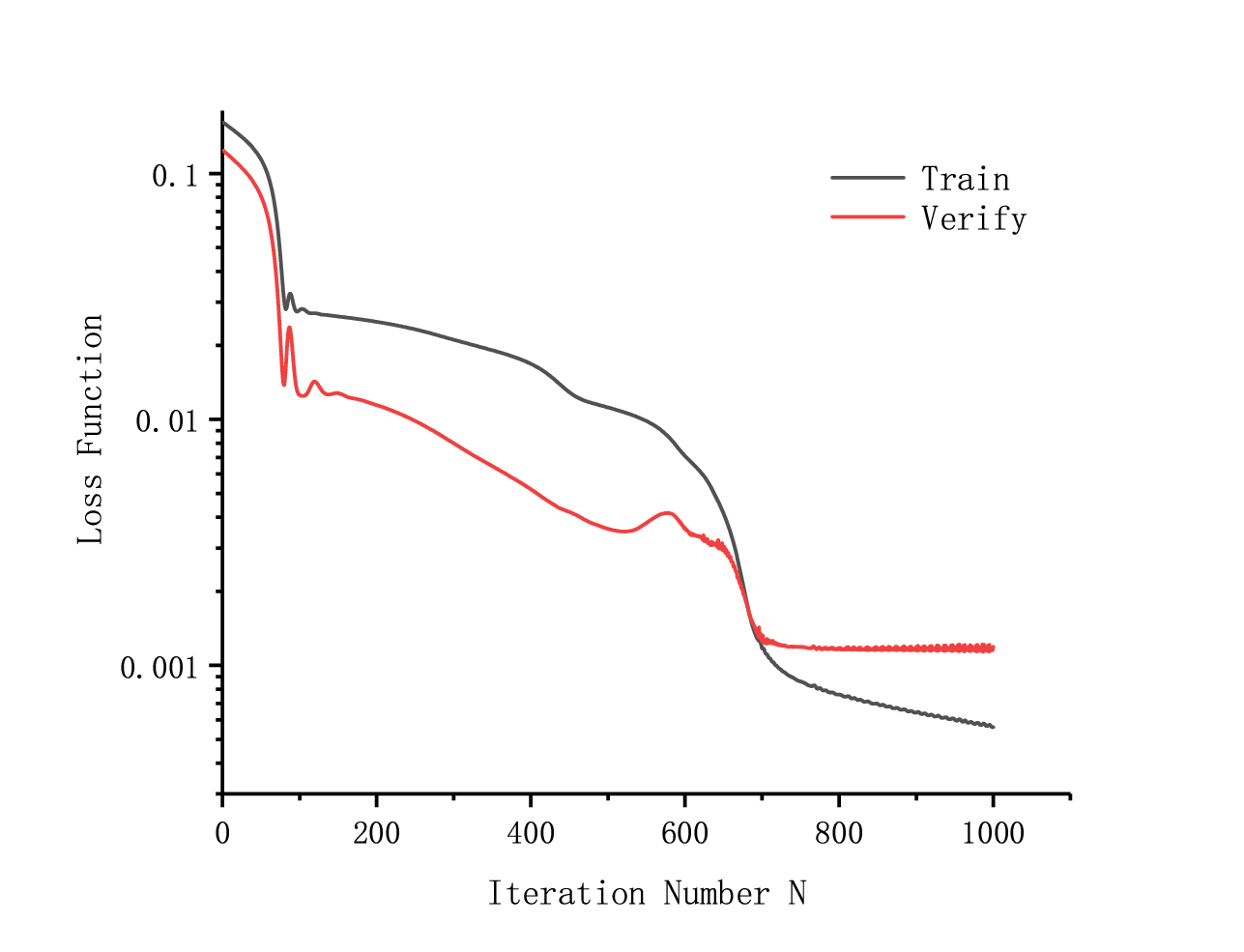
The loss function is checked in the neural network module, verifying the robustness of the model. Figure 5 is an exemplary. It shows the variation of loss function with iteration number during the training of the model for . Black curve represents the loss function between measurement and the prediction from the model, while the red curve represents the loss function between verification measurement and the prediction from the model. As is shown, the loss function drops logarithmically with the iteration number. As is seen in the Figure 5 both of them drop to order of magnitude after roughly 700 iterations. This is double-confirmed in Figure 6Wang et al. 2020. The measured used for tranining, the predicted by the trained model using neural network, and the measured based on trained model for its verification are all plotted to the measured used for tranining. For both and , the predicted value (blue rectangle), and the verify data (red circle) are in close vicinity with the measurement (black line), proving the accuracy and robustness of the model.
The results output from the trained model can be visualized by Figure 7, which shows the three-dimensional view for and as the function of normalized and , respectively. It can be noted that in the investigated parameter space of and , both and has a valley shape, indicating minimum and exist and have been searched out for proper combination of and by the trained model.
From these measurements, we performed such proof-of-principle tests using two voltage inputs and two outputs for the training using neural network. We further extended such tests with three voltage inputs and four voltage inputs . With these inputs, we performed similar training to the model using neural network, and verified accuracy of the trained model. As shown in Figure 8, the predicted value (blue rectangle), and the verify data (red circle) agree well with the measurement (black line), demonstrating the accuracy of the trained model.


For four voltage inputs, we found the global minimum of and for a specific combination of . The generated photon-correlation spectrum is shown in Figure 9. The corresponding and are inferred to and by fitting the photon-correlation spectrum in Figure 9 to the Equation 8. Such order of magnitude show an excellent minimization and is comparable to Berkeland et al. 1998; Keller et al. 2015, clearly demonstrating the efficacy of machine learning in this application. In addition, we reached the same results with decision tree, another widely used algorithm in machine learning.


Conclusion
we have demonstrated a high-level of micromotion suppression by neural-network based machine learning, using RF-photon correlation technique. With our approach, both and have been reduced to order of magnitude, reaching state-of-the-art sensitivity and comparable to the those used for atomic clocks Berkeland et al. 1998; Keller et al. 2015 and quantum metrology. is estimated to within according to its relation with , as discussed in the section of theoretical scheme. We also envision that this approach can be generally applied to other similar scenarios in atomic, molecular and optical physics, quantum information processing, and quantum computation.
Acknowledgement
Yang Liu acknowledge the financial support from National Natural Science Foundation of China(NSFC) under Grant No. 11974434, Fundamental Research Funds for the Central Universities of Education of China under Grant No. 191gpy276, Natural Science Foundation of Guangdong Province under Grant 2020A1515011159. Le Luo received supports from NSFC under Grant No.11774436, Guangdong Province Youth Talent Program under Grant No.2017GC010656, Sun Yat-sen University Core Technology Development Fund, and the Key-Area Research and Development Program of GuangDong Province under Grant No.2019B030330001.
References
- Awad and Khanna (2015) M. Awad and R. Khanna, Efficient learning machines: theories, concepts, and applications for engineers and system designers (Springer nature, 2015).
- Arsenault et al. (2014) L.-F. Arsenault, A. Lopez-Bezanilla, O. A. von Lilienfeld, and A. J. Millis, Physical Review B 90, 155136 (2014).
- Rupp (2015) M. Rupp, International Journal of Quantum Chemistry 115, 1058 (2015).
- Li et al. (2015) Z. Li, J. R. Kermode, and A. De Vita, Physical review letters 114, 096405 (2015).
- Pilania et al. (2016) G. Pilania, A. Mannodi-Kanakkithodi, B. Uberuaga, R. Ramprasad, J. Gubernatis, and T. Lookman, Scientific reports 6, 1 (2016).
- Carrasquilla and Melko (2017) J. Carrasquilla and R. G. Melko, Nature Physics 13, 431 (2017).
- Raissi and Karniadakis (2018) M. Raissi and G. E. Karniadakis, Journal of Computational Physics 357, 125 (2018).
- Radovic et al. (2018) A. Radovic, M. Williams, D. Rousseau, M. Kagan, D. Bonacorsi, A. Himmel, A. Aurisano, K. Terao, and T. Wongjirad, Nature 560, 41 (2018).
- Carleo et al. (2019) G. Carleo, I. Cirac, K. Cranmer, L. Daudet, M. Schuld, N. Tishby, L. Vogt-Maranto, and L. Zdeborová, Reviews of Modern Physics 91, 045002 (2019).
- Sarma et al. (2019) S. D. Sarma, D.-L. Deng, and L.-M. Duan, arXiv preprint arXiv:1903.03516 (2019).
- Schütt et al. (2020) K. T. Schütt, S. Chmiela, O. A. von Lilienfeld, A. Tkatchenko, K. Tsuda, K.-R. Müller, Schütt, and Scalone, Machine Learning Meets Quantum Physics (Springer, 2020).
- Goh et al. (2017) G. B. Goh, N. O. Hodas, and A. Vishnu, Journal of computational chemistry 38, 1291 (2017).
- Kitchin (2018) J. R. Kitchin, Nature Catalysis 1, 230 (2018).
- Butler et al. (2018) K. T. Butler, D. W. Davies, H. Cartwright, O. Isayev, and A. Walsh, Nature 559, 547 (2018).
- Tkatchenko (2020) A. Tkatchenko, Nature Communications 11, 1 (2020).
- Cartwright (2020) H. M. Cartwright, Machine Learning in Chemistry, Vol. 17 (Royal Society of Chemistry, 2020).
- Tarca et al. (2007) A. L. Tarca, V. J. Carey, X.-w. Chen, R. Romero, and S. Drăghici, PLoS Comput Biol 3, e116 (2007).
- Angermueller et al. (2016) C. Angermueller, T. Pärnamaa, L. Parts, and O. Stegle, Molecular systems biology 12, 878 (2016).
- Ching et al. (2018) T. Ching, D. S. Himmelstein, B. K. Beaulieu-Jones, A. A. Kalinin, B. T. Do, G. P. Way, E. Ferrero, P.-M. Agapow, M. Zietz, M. M. Hoffman, et al., Journal of The Royal Society Interface 15, 20170387 (2018).
- Ball and Brunner (2010) N. M. Ball and R. J. Brunner, International Journal of Modern Physics D 19, 1049 (2010).
- Way et al. (2012) M. J. Way, J. D. Scargle, K. M. Ali, and A. N. Srivastava, Advances in machine learning and data mining for astronomy (CRC Press, 2012).
- VanderPlas et al. (2012) J. VanderPlas, A. J. Connolly, Ž. Ivezić, and A. Gray, in 2012 conference on intelligent data understanding (IEEE, 2012) pp. 47–54.
- Ivezić et al. (2014) Ž. Ivezić, A. J. Connolly, J. T. VanderPlas, and A. Gray, Statistics, data mining, and machine learning in astronomy: a practical Python guide for the analysis of survey data, Vol. 1 (Princeton University Press, 2014).
- Baron (2019) D. Baron, arXiv preprint arXiv:1904.07248 (2019).
- Herbrich et al. (1999) R. Herbrich, M. Keilbach, T. Graepel, P. Bollmann-Sdorra, and K. Obermayer, in Computational techniques for modelling learning in economics (Springer, 1999) pp. 169–196.
- Mullainathan and Spiess (2017) S. Mullainathan and J. Spiess, Journal of Economic Perspectives 31, 87 (2017).
- Athey (2018) S. Athey, in The economics of artificial intelligence: An agenda (University of Chicago Press, 2018) pp. 507–547.
- Bose and Mahapatra (2001) I. Bose and R. K. Mahapatra, Information & management 39, 211 (2001).
- Khandani et al. (2010) A. E. Khandani, A. J. Kim, and A. W. Lo, Journal of Banking & Finance 34, 2767 (2010).
- Heaton et al. (2017) J. B. Heaton, N. G. Polson, and J. H. Witte, Applied Stochastic Models in Business and Industry 33, 3 (2017).
- Klaas (2019) J. Klaas, Machine learning for finance: principles and practice for financial insiders (Packt Publishing Ltd, 2019).
- Lai et al. (2004) L. L. Lai, H. Braun, Q. Zhang, Q. Wu, Y. Ma, W. Sun, and L. Yang, in Proceedings of 2004 International Conference on Machine Learning and Cybernetics (IEEE Cat. No. 04EX826), Vol. 7 (IEEE, 2004) pp. 4216–4221.
- Sharma et al. (2011) N. Sharma, P. Sharma, D. Irwin, and P. Shenoy, in 2011 IEEE international conference on smart grid communications (SmartGridComm) (IEEE, 2011) pp. 528–533.
- Kendon et al. (2014) E. J. Kendon, N. M. Roberts, H. J. Fowler, M. J. Roberts, S. C. Chan, and C. A. Senior, Nature Climate Change 4, 570 (2014).
- Choi et al. (2016) S. Choi, Y. J. Kim, S. Briceno, and D. Mavris, in 2016 IEEE/AIAA 35th Digital Avionics Systems Conference (DASC) (IEEE, 2016) pp. 1–6.
- Holmstrom et al. (2016) M. Holmstrom, D. Liu, and C. Vo, Meteorol. Appl (2016).
- Kononenko (2001) I. Kononenko, Artificial Intelligence in medicine 23, 89 (2001).
- Raccuglia et al. (2016) P. Raccuglia, K. C. Elbert, P. D. Adler, C. Falk, M. B. Wenny, A. Mollo, M. Zeller, S. A. Friedler, J. Schrier, and A. J. Norquist, Nature 533, 73 (2016).
- Ward et al. (2016) L. Ward, A. Agrawal, A. Choudhary, and C. Wolverton, npj Computational Materials 2, 1 (2016).
- Ramprasad et al. (2017) R. Ramprasad, R. Batra, G. Pilania, A. Mannodi-Kanakkithodi, and C. Kim, npj Computational Materials 3, 1 (2017).
- Sanchez-Lengeling and Aspuru-Guzik (2018) B. Sanchez-Lengeling and A. Aspuru-Guzik, Science 361, 360 (2018).
- Schmidt et al. (2019) J. Schmidt, M. R. Marques, S. Botti, and M. A. Marques, npj Computational Materials 5, 1 (2019).
- Deo (2015) R. C. Deo, Circulation 132, 1920 (2015).
- Obermeyer and Emanuel (2016) Z. Obermeyer and E. J. Emanuel, The New England journal of medicine 375, 1216 (2016).
- Seif et al. (2018) A. Seif, K. A. Landsman, N. M. Linke, C. Figgatt, C. Monroe, and M. Hafezi, Journal of Physics B: Atomic, Molecular and Optical Physics 51, 174006 (2018).
- Chwalla (2009) M. M. Chwalla, Precision spectroscopy with 40 Ca ions in a Paul trap, Ph.D. thesis, PhD thesis, Universität Innsbruck (2009).
- Doret et al. (2012) S. C. Doret, J. M. Amini, K. Wright, C. Volin, T. Killian, A. Ozakin, D. Denison, H. Hayden, C. Pai, R. E. Slusher, et al., New Journal of Physics 14, 073012 (2012).
- Narayanan et al. (2011) S. Narayanan, N. Daniilidis, S. Möller, R. Clark, F. Ziesel, K. Singer, F. Schmidt-Kaler, and H. Häffner, Journal of Applied Physics 110, 114909 (2011).
- Tanaka et al. (2012) U. Tanaka, K. Masuda, Y. Akimoto, K. Koda, Y. Ibaraki, and S. Urabe, Applied Physics B 107, 907 (2012).
- Berkeland et al. (1998) D. J. Berkeland, J. D. Miller, J. C. Bergquist, W. M. Itano, and D. J. Wineland, Journal of Applied Physics 83, 5025 (1998).
- Keller et al. (2015) J. Keller, H. L. Partner, T. Burgermeister, and T. E. Mehlstäubler, Journal of Applied Physics 118, 104501 (2015), arXiv:1505.05907 [physics.atom-ph] .
- Leibfried et al. (2003) D. Leibfried, R. Blatt, C. Monroe, and D. Wineland, Reviews of Modern Physics 75, 281 (2003).
- Riehle (2006) F. Riehle, Frequency standards: basics and applications (John Wiley & Sons, 2006).
- Mohri et al. (2018) M. Mohri, A. Rostamizadeh, and A. Talwalkar, Foundations of machine learning (MIT press, 2018).
- Russell and Norvig (2002) S. Russell and P. Norvig, (2002).
- Hinton et al. (1999) G. E. Hinton, T. J. Sejnowski, et al., Unsupervised learning: foundations of neural computation (MIT press, 1999).
- Kaelbling et al. (1996) L. P. Kaelbling, M. L. Littman, and A. W. Moore, Journal of artificial intelligence research 4, 237 (1996).
- Nair and Hinton (2010) V. Nair and G. E. Hinton, in Icml (2010).
- Goodfellow et al. (2016) I. Goodfellow, Y. Bengio, A. Courville, and Y. Bengio, Deep learning, Vol. 1 (MIT press Cambridge, 2016).
- Bottou (1998) L. Bottou, On-line learning in neural networks 17, 142 (1998).
- Kiwiel (2001) K. C. Kiwiel, Mathematical programming 90, 1 (2001).
- Orr and Müller (2003) G. B. Orr and K.-R. Müller, Neural networks: tricks of the trade (Springer, 2003).
- Johnson et al. (2016) K. G. Johnson, J. D. Wong-Campos, A. Restelli, K. A. Landsman, B. Neyenhuis, J. Mizrahi, and C. Monroe, Review of Scientific Instruments 87, 053110 (2016), arXiv:1603.05492 [physics.atom-ph] .
- Wang et al. (2020) R. Wang, A.-L. Luo, J.-J. Chen, W. Hou, S. Zhang, Y.-H. Zhao, X.-R. Li, Y.-H. Hou, L. M. Collaboration, et al., The Astrophysical Journal 891, 23 (2020).