Projection-tree reduced order modeling for fast -body computationsJournal: Elsevier
Abstract
This work presents a data-driven reduced-order modeling framework to accelerate the computations of -body dynamical systems and their pair-wise interactions. The proposed framework differs from traditional acceleration methods, like the Barnes–Hut method, which requires online tree building of the state space, or the fast-multipole method, which requires rigorous a priori analysis of governing kernels and online tree building. Our approach combines Barnes-Hut hierarchical decomposition, dimensional compression via the least-squares Petrov–Galerkin (LSPG) projection, and hyper-reduction by way of the Gauss-Newton with approximated tensor (GNAT) approach. The resulting projection-tree reduced order model (PTROM) enables a drastic reduction in operational count complexity by constructing sparse hyper-reduced pairwise interactions of the -body dynamical system. As a result, the presented framework is capable of achieving an operational count complexity that is independent of , the number of bodies in the numerical domain. Capabilities of the PTROM method are demonstrated on the two-dimensional fluid-dynamic Biot-Savart kernel within a parametric and reproductive setting. Results show the PTROM is capable of achieving over 2000 wall-time speed-up with respect to the full-order model, where the speed-up increases with . The resulting solution delivers quantities of interest with errors that are less than 0.1% with respect to full-order model.
Keywords:
Reduced-order modeling, LSPG, GNAT, tree algorithms, Barnes–Hut, hyper-reduction1 Introduction
Lagrangian and discrete -body computational modeling, or meshless computational modeling, of dynamical systems are ubiquitous across different disciplines in science and engineering. For instance, vortex methods, such as the free-vortex wake method (FVM) [53, 56, 57, 58, 54, 63, 28], the vortex panel and particle methods [35, 19, 38, 22, 23], are commonly used in the aerospace community to capture the near-wake dynamics of rotorcraft and fixed-wing aircraft. The smooth particle hydrodynamic (SPH) method provides effective modeling in fluids [68], additive manufacturing [61], and has even been used to model cosmological shock waves [52] and dark matter halos [45]. The discrete element method (DEM) has been used to simulate the thermomechanical states of additive manufacturing [66], and has also been used to simulate complex granular flow [37]. The molecular dynamics (MD) method [33, 48, 71, 20], which is akin to DEM, has been used to model the physical movements of atoms and molecules. These computational methods are often employed due to their many benefits, such as bypassing Eulerian grid-based artificial numerical dissipation [41], tracking individual particle time histories [42], enabling constitutive behavior not available in grid-based (continuum) methods [66], and modeling of multiphase multiphysics, free-surface flow, and splash with complex geometries [64]. Unfortunately, discrete computational -body methods suffer from poor operational count complexity (OCC) associated with pairwise interactions that generally scale quadratically, , or super-linearly, , where is the number of bodies in the computational domain, and , such that is a mapping that dictates the neighbor particle count for each -body, which tends to be much higher than neighboring nodes in traditional mesh-based methods.
Many research efforts have been dedicated to reducing the cost of computational methods based on -body pairwise interactions [74], where the most successful and general effort has been the fast multipole method (FMM) [30], which was named one of the top ten algorithms of the century [18, 21]. The FMM computes a multipole expansion of the field potential and executes a hierarchical decomposition to separate near-field from far-field particles. The influence of far-field particles is then approximated by lower order terms, and the far-field particles are grouped together to form fewer but stronger particles in the far field domain. The FMM approximation can at best reduce OCC to a linear scaling, with respect to the number of particles in the domain [74]. However, FMM has drawbacks in application. For instance, the FMM can be very difficult to implement in three-dimensions, can be kernel dependent (i.e. not all Greens functions are FMM adaptable), and the multipole expansion computation of the field potential is costly [29, 74]. Kernel independent variants of the FMM exist, which aim to reduce the cost of the field potential computation independent of the kernel type, for example see [44, 73, 36]. However, for dynamical simulations the FMM and its variants are ultimately bounded by OCC that depends on multiple online updates of the hierarchical decomposition, and depend on potential field computations over all particles in the domain, i.e. FMM-based methods are at best or “".
In contrast, acceleration methods based on Lagrangian counterparts, i.e. Eulerian grid-based methods, have achieved complexity reduction independent of the number of nodal degrees-of-freedom in the computational domain, i.e. -independent. This -independent complexity reduction has been achieved by means of data-driven projection reduced order modeling (PROM) for applications in multi-query loops, i.e., optimization, control, uncertainty quantification, and inverse problems, where a non-exhaustive list of these developments are included in [16, 15, 14, 26, 27, 59, 60, 5, 8, 11]. The objective of PROM is to perform dimensional compression by learning about a dynamical system’s solution manifold and determine a corresponding low-dimensional embedding (mappings from high-dimensions to low-dimensions) where the system’s governing equation can be computed. Finding the dynamical system’s low-dimensional embedding is performed a priori, during an off-line training stage, which scales with the intrinsic dimension of the solution manifold under consideration, i.e. offline stages are -dependent. In PROM, finding the system’s low-dimensional embedding is enabled by projection methods such as Galerkin [65, 14], Petrov-Galerkin [13, 3], or least-square Petrov-Galerkin projection [16, 14]. Once the low-dimensional embedding has been discovered, the PROM can deployed on-line to perform rapid -independent computations for multiquery setting, such as design optimization, control, uncertainty quantification and inverse problems.
Traditionally in PROM, the embedding is generated by an affine subspace approximation, a reduced basis, of the entire solution manifold (a data-driven global basis function). A non-exhaustive list of methods that construct these subspace approximations include the proper orthogonal decomposition (POD) [65, 34, 60], balanced POD [59, 72], symplectic POD [50, 32, 1], reduced basis method [31, 12], and dynamic mode decomposition (DMD) [62, 70, 39, 24, 46]. Taira et al. 2017 provide a great overview and review of popular projection techniques widely used in PROMs. Other methods exist to alleviate the strong affine approximation over the solution manifold, which can be nonlinear, by finding local affine approximations (akin to linearly discretizing over the solution manifold), such as the local reduced order basis method [4]. Recent works have also taken advantage of new developments in convolutional deep neural networks to determine optimal nonlinear, global, and low-dimensional embeddings to overcome strong affine approximations and Kolmogorov width limitations [40]. Brunton and Kutz 2019 provide a great overview and introduction to these machine-learning and PROM techniques used in nonlinear dynamical systems. From a general and overhead perspective, PROM can be perceived as a data-driven Ritz method, where the basis function is determined from a dynamical system’s data a posteriori and is used to project the full-order system of equations onto a low-dimensional embedding that approximates the dynamical system behavior.
For nonlinear dynamical systems, identifying a low-dimensional embedding is often not enough to enable -independent computations, due to persistent high dimensional, higher-order, non-linear, and parametrized dependencies of the underlying system of equations. As a result, nonlinear PROMs are often accompanied by additional layers of complexity reduction, known as hyper-reduction, which alleviate the embedded system from the persistent high-dimensional dependence after projection is performed. In essence, hyper-reduction enables the computation of dynamical system’s evolution in the low-dimensional embedding over a sparse set of sampled points in the numerical domain. A non-exhaustive list of these hyper-reduction methods include the emperical interpolation method (EIM) [7], discrete EIM (DEIM) [17], unassembled DEIM (UDEIM) [69], Gauss-Newton with approximated tensors (GNAT) [16], and energy conserving sampling and weighing (ECSW) [26, 27].
To the best of the authors’ knowledge, PROM approaches developed for Eulerian grid-based methods have not been cast into an effective -independent Lagrangian framework for -body problems until the work presented herein. This paper presents an OCC-reducing framework that employs hierarchical decomposition to reduce pairwise interaction operation counts, projection based dimensionality reduction, and hyper-reduction to perform a sparse set of pairwise interactions. The method presented in this work can be perceived as a data-driven kernel independent acceleration algorithm, where hierarchical decomposition occurs once offline and the kernel is approximated via a sparse representation of LSPG projection, all of which delivers an -independent acceleration framework for -body problems.
The remainder of this paper is organized as follows. Section 2 presents the problem formulation. Specifically, the two-dimensional Biot–Savart kernel is presented in the form of a parametric ordinary differential equation (ODE). Section 3 introduces projection-based reduced order modeling, specifically the least-squares Petrov-Galerkin projection. Section 4 introduces the Barnes–Hut quad-tree (two-dimensional) hierarchical decomposition method. The main contribution of this work, i.e. the PTROM, is presented in Section 5. Applications of the presented PTROM framework in the form of reproductive and parametric studies are presented Section 6. Finally, conclusions and future directions are offered in Section 7.
2 Problem Formulation
Development of the PTROM in this work is rooted in the Biot–Savart kernel, which is often used to model vorticity transport in fluid-dynamics as an -body problem. The Biot–Savart kernel is often used as the underlying theoretical foundation for many Lagrangian computational fluid-dynamics frameworks, such as the vorticity transport model (VTM) [9], FVM [63, 55, 56, 57], and many others [35, 19, 38, 2]. The overarching goal of this work is to develop the mathematical foundations of the PTROM using the Biot–Savart kernel, but to maintain a general structure of the formulation, such that any other -body kernel could be substituted in the presented framework. In this paper, the Biot–Savart kernel and its -body pair-wise full-order model (FOM) is presented for a two-dimensional study in the form of a time-continuous ordinary differential equation (ODE). For a particle, , the ODE formulation is defined by
| (1) |
where , is the position vector of the particle and and are the two-dimensional Cartesian coordinates. Here, denotes time with the final time , is the parameter container of all particles (i.e., contains circulation or density), is the number of particles, the second equality in Eq. 1 defines the initial conditions, and superscript denotes the transpose operations. Here, is the Biot–Savart kernel,
| (2) |
where is the circulation, and is the out-of-plane unit normal vector of the body, and is the de-singularization constant where . The kernel outputs are denoted by where the subscripts and denote the and output components. For the current two-dimensional study, it is convenient to introduce that collects the particle positions in a vector such that , with , where refers to our two-dimensional system, and where . Similarly, we introduce that collects the particle velocity in a vector such that , and . As a result the particle-wise ODE formulation in Eq. 1 can be rewritten into a traditional vector ODE form:
| (3) |
where denotes the time-dependent parameterized state, which is implicitly defined as the solution to the full -body pair-wise interaction problem in Eq. 3, with parameters . Here, denotes the parameter space of parameters, and is the parametrized initial condition. Finally, which denotes the vector of velocity components generated by the kernel .
It is also useful to arrange the Biot-Savart law pair-wise interaction in block-matrix form. Let
| (4) |
where . Next, a block matrix is formed such that
| (5) |
where
| (6) |
and . The two-dimensional Biot-Savart kernel can then be written as
| (7) |
which helps contextualize the pair-wise interactions with the “target-source" relationship. Figure 1 illustrates an example of the target-source relationship of a tip-vortex shed off of an elliptical wing formed in with the Biot–Savart kernel, where the three-dimensional dynamics have been projected on a two-dimensional plane. Through-out this paper, the pre-defined circulation of the particles will serve as parametric variables, as will be shown in Section 6.

The two-dimensional dynamical system presented in Eq. 3 can be discretized in time by a -step linear multistep scheme, where denotes the number of steps in the multistep scheme and , in residual form as:
| (8) |
where the superscript designates the value of a variable at time step , denotes the final number of time steps taken, and . The time-discrete residual is defined as
| (9) |
where the current work employs the implicit trapezoidal rule, such that . Furthermore, the time step is denoted by and is considered uniform. Here, denotes the numerical approximation to , and is the unknown state vector that is implicitly solved to explicitly update the state, i.e. . Finally, the implicit trapezoidal integration employed herein is solved via an inexact Newton method, such that the Jacobian is updated every time-steps, where and . It is also important to note that the current work introduces an inexact kernel Jacobian to compute the residual Jacobian, where only the diagonal block entries are computed, i.e. . This inexact approach is performed to avoid computing a fully-populated matrix where the off-diagonal blocks of the kernel Jacobian provide neglible contributions to the residual Jacobian.
3 Projection-based reduced order modeling
To enable rapid computations of the -body problem in a low-dimensional embedding, the presented PTROM performs dimensional compression of Eq. 9 via the least-squares Petrov–Galerkin (LSPG) projection [16, 14]. Specifically, the PTROM seeks an approximate solution, , of the form
| (10) |
where and denotes some trial manifold. Here denotes some parameterized reference state and with and denotes a parameterization function that projects or maps the low-dimensional generalized coordinates to the high-dimensional approximation, .
The current work focuses only on constructing an affine trial manifold that exist in the Steifel manifold, i.e. for a full-column-rank matrix, , the Steifel manifold is defined by . This affine manifold is expressed as , where , where the current work constructs a POD [34] basis matrix as the mapping operator, . Finally, for the current POD basis, the reference state can be set as , and so the full-order model state vector can be approximated as
| (11) |
It’s important to note that although the current work has been restricted to affine trial manifolds, recent works in [40] have generalized projection based dimensionality compression via nonlinear trial manifolds. Future work will look into generalizing the PTROM framework by adopting these nonlinear mappings, as they have shown to out-perform POD bases for advection dominated physics.
3.1 Constructing the proper-orthogonal decomposition basis
As previously mentioned, the projection operator, , is based on constructing the POD basis which is a main tool for building the PTROM. Thus, the POD construction procedure will be discussed here. To build , the method of snapshots is employed, where the singular-value decomposition (SVD) is used to factor the snapshot data matrix , where
| (12) |
and where columns of represent the time history of the state vector, . By factoring the snapshot matrix via the SVD, we obtain
| (13) |
where the left-singular matrix , the singular-value matrix has diagonal entries that follow a monotonic decrease such that, , and the right-singular matrix . The POD basis used to build the low-dimensional subspace is constructed by taking the left singular vectors of , such that where . Constructing this POD basis is performed as a training step a priori, before any online simulations are performed.
3.2 Least-Squares Petrov–Galerkin projection
The least-squares Petrov–Galerkin (LSPG) method constructs a projection-based and time-discrete residual minimization framework, where the projection-based state approximation, Eq. 11, is substituted into the time-discrete residual, Eq. 9, and cast into a nonlinear least-squares formulation. The LSPG method provides discrete optimality of the residual, , at every time-step [16], such that
| (14) |
It can be shown that this time-discrete residual minimization is akin to a Petrov-Galerkin projection at the time-discrete level, where the test basis is defined by the residual Jacobian and the trial basis is the familar POD basis, , such that , hence the name “least-squares Petrov–Galerkin projection".
The solution to Eq. 14 yields the following iterative linear least-squares formulation via the Gauss-Newton method:
| (15) |
and updates to the iterative solution are given by
| (16) |
for and where denotes a step length in the search direction, , that can be computed to ensure global convergence (e.g., satisfy the strong Wolfe conditions [47]). Here, the initial guesses for the iterative problem are taken as .
3.3 Hyper-reduction
Despite the low-dimensional sub-space of the generalized coordinates and trial manifold, for all time steps the LSPG method requires the evaluation of residual minimization operations and pair-wise operations of the kernel. Therefore, a layer of reduction is required to reduce the OCC of the residual minimization counts in Eq. 15 and 16. The current PTROM employs hyper-reduction to perform sparse residual minimization. Specifically the GNAT hyper-reduction approach [16] is employed, which performs LSPG residual minimization on a weighted -norm, such that
| (17) |
Here, the weighting matrix, , is constructed by a gappy POD approach [25], where the time-discrete residual is approximated and minimized over a sparse set of entries. The residual approximation, , is constructed by way of a time-discrete residual POD basis employing the offline training procedure discussed in Section 3.1, where , such that , , and is the number of retained SVD singular vectors in . Next, the residual minimization over a sparse set of entries is performed by the following linear least-squares problem,
| (18) |
where the matrix is a sampling matrix consisting of sparse selected rows of the identity matrix, which also correspond to the same rows in the time-discrete residual vector, where . Note is the number of sparsely sampled particles, and , which correspond to the number of sparsely sampled degrees-of-freedom. The solution to Eq.18 yields
| (19) |
Substituting Eq. 19 into yields the residual approximation
| (20) |
whereby via the approximation, , the substitution of Eq. 20 into the weighted LSPG minimization in Eq. 17 yields the following residual minimization,
| (21) |
where . A visual representation of the GNAT hyper-reduction technique employed for -body pair-wise interactions is illustrated in Fig. 2 below.
3.4 Constructing the sampling matrix
To enable the sparse residual minimization of Eq. 21, a sampling matrix is constructed strategically. Work presented in [16] constructed a sampling matrix tailored to a computational fluid dynamics (CFD) mesh via a greedy algorithm based on mitigating the maximum error of the POD residual basis and POD residual Jacobian basis. The current sampling approach is similar to that presented in [16] but is tailored to a computational domain for -body problems and only attempts to mitigate the error of the POD residual basis. The greedy algorithm to construct the sampled matrix is presented below in Algorithm 1.
Compute additional number of bodies left to sample
Initialize counter for the number of working basis vectors used:
Set the number of greedy iterations to perform:
Compute the maximum number of right-hand sides in the least-squares problem:
Compute the minimum number of working basis vectors per iteration:
Compute the minimum number of sample bodies to add per iteration:
for = do // begin greedy sampeling loop 1
if then 2
if and then 4
// where denotes the degrees of freedom associated with the body
end for 11
ensures the system of equations in the minimization problem remains over-determined 14
3.5 Remarks on the current projection-based reduced reduced order model
Implementing GNAT hyper-reduction into an LSPG method drastically reduces the residual minimization count over the residual vector space. For grid-based methods, this hyper-reduction step is sufficient to achieve -independence. However, employing GNAT hyper-reduction on computational Lagrangian -body methods only reduces the number of target bodies in the -body pairwise interaction, which still requires the knowledge of all sources in the domain that act on targets. Therefore, even though integrating GNAT hyper-reduction into the -body problem reduces overall OCC, the resulting cost remains -dependent, and requires an additional layer of reduction to reduce the number of sources.
4 The Barnes–Hut tree method
Prior sections focused on drastically decreasing OCC and compute-time by finding a low-dimensional embedding over a hyper-reduced numerical domain. Now, it also necessary to reduce the OCC dependencies associated with sources over the sparse residual entries in Eq. 21 to realize -independence and further improve the efficiency of the current framework. Here, the PTROM employs hierarchical decomposition and source agglomeration via the Barnes–Hut tree method [6, 51]. The Barnes–Hut tree method builds a hierarchical quad-tree (or in three-dimension, oct-tree) data structure, , that performs recursive partitioning over the entire domain (the root node) that contains all bodies. Recursive partitioning generates branch nodes until a desired number of bodies are contained per partition, where this final level of partitioning is known as the leaf node. Figure 3 illustrates the hierarchical data-structure generated by the Barnes–Hut tree method. The Barnes–Hut tree method is well-documented in the literature, where pseudo codes and flowcharts to build the hierarchical data structure can be found in [51].
4.1 Source clustering
The Barnes–Hut data structure enables OCC reduction by employing branch node agglomeration that correspond to negligible far-field sources. The PTROM explores two criteria to identify which branch nodes to cluster: 1) A neighbor search criteria, and 2) the classical Barnes–Hut clustering criteria. Before presenting the details of the clustering criteria, useful terminology is introduced:
Definition 1.
Let the Cartesian position vector of a target be expressed by . Next, let the set of far-field sources be expressed by , and let denote the surrogate source representing the clustered set . The Cartesian position vector for a source in the set , is defined by , and so the Cartesian position vector for the surrogate source is defined by some weighted mean, , where the subscripts and denote Cartesian coordinate components of and is the cardinality of . Note that the weighted mean is computed within the context of the Biot–Savart kernel, such that the circulation of source bodies in correspond to the weights in the mean computations.
Definition 2.
Let denote the quad-tree quadrilateral source node containing . The width of is defined as the maximum length of its sides, and node contains all inside the boundary and , where is the set of boundaries of and its components are in . Similarly, let denote the quad-tree quadrilateral leaf node containing a set of targets, , where the position vector for an target in is defined by . The width of is defined as the maximum length of its sides, and node contains all inside the boundary and , where is the set of boundaries of and its components are in . Finally, the neighborhood of the target node, , is defined by the following set of boundaries , where each component of is in , , is a factor that is added to the target node boundaries to extend the neighborhood of the target node, and denotes the direct sum.
The neighbor search criteria employed by the PTROM is based on identifying any overlapping source node corners, within the neighborhood boundaries of a target node. Specifically, clustering occurs if, and only if, a source node corner does not overlap with a target neighborhood, i.e. must all be false to cluster. The Barnes–Hut clustering criteria is based on clustering when the following is met: If , where and is a user-defined clustering parameter, then clustering of is performed. An illustration of the two clustering approaches is shown in Fig. 4. A pseudo algorithm for both clustering approaches will be provided in the proceeding sub-section.
4.1.1 Hierarchical decomposition of the projection basis
Traditionally, computing the Barnes-Hut tree decomposition and corresponding source clustering is performed over the -body state-space, where both tree decomposition and clusters are updated at incremental time-steps throughout a simulation. However, building the tree data structure and performing source clustering are -dependent operations [51], which would not overcome the -dependent OCC barrier in the hyper-reduction step, as discussed in Section 3.5. To overcome the need to perform multiple online tree construction and clustering of the state space the PTROM constructs the hierarchical data structure and source clustering in a weighted POD space, offline and only once. This weighted POD space is denoted by , where and its entries correspond to the diagonal entries of up to the retained singular value. In other words, is a linear combination of the POD trial bases where the weights are defined by the corresponding singular values of the retained columns in the singular matrix, . Figure 5 illustrates the offline procedure to compute the weighted POD space, construct the data structure, , and perform source clustering.
By computing the hierarchical decomposition and clustering in , all clusters and nodes identified over the particle domain can be mapped to associated degrees-of-freedom per column in the POD basis matrix, . This mapping of the degrees-of-freedom from to allows the construction of a “source surrogate POD basis" data structure that reduces the dimensionality of by approximating the structure of the source POD mode shapes as observed by the sparsely sampled targets selected by Algorithm 1, which ultimately enables -independence. Mapping from to and the associated construction of the source surrogate POD basis is depicted in Figure 6, where the algorithm to perform the construction of the surrogate POD basis data structure is presented in Algorithm 2.The construction of occurs during the clustering of , such that the degrees of freedom clustered in the weighted POD space are mapped to corresponding row entries of , and these associated row entries of are clustered to generate .
As mentioned earlier, the data-structure contains approximations of POD modes as observed by individual sampled targets. In other words, contains a library of POD mode source approximations for all sampled targets. Figure 7 compares the interaction between a sampled target, say particle , and all source POD modes against the interaction between a sampled target and clustered source POD modes. It is important to take notice that clusters of the POD modes in the weighted space are generally not unique for each sampled target. In fact, most targets in the same neighborhood share the same clusters. As a result, there exists a unique number of source POD surrogate clusters, and corresponding degree-of-freedom for all sampled targets, where and and . These unique source POD structures can then be structured into the final form of the source POD basis surrogate matrix, . Similarly, the same unique clusters have a unique agglomerated circulation, which must also be structured into the compact vector , where is the number of unique source strengths and . The process of finding unique source POD surrogate clusters is straight-forward and there is no specific search algorithm that must be used. As a result, Algorithm 2 denotes the unique cluster search by the function UniqueSearch.
1
3
6
for k=1 …4 do // cluster the children of this node 9
11
while do 20
if Prune = False then // if false, check children for pruning instead 22
for j=1 …4 do 23
36
if Prune Technique = “Barnes–Hut" then 1
if then 2
query the target node boundaries from see Def. 2
query the source node boundaries from , see Def. 2
define the neighborhood of the target, see Def. 2.
// Check overlap between target and source cells:
overlap and
overlap and
end if 8
5 Projection-tree reduced order modeling
The combination of projection-based dimensionality reduction, hyper-reduction, and tree-based hierarchical decomposition constitutes the presented “projection-tree reduced order model" to rapidly compute -body problems. Figure 8 illustrates the underlying concept of the PTROM framework, which is a sparse residual minimization problem in a low-dimesional embedding over a clustered set of sources. In this section, a discussion on the training hierarchy is presented, along with a presentation of the deployed online computations, discussions on the independent OCC, and error bounds of the resulting framework.
5.1 Training hierarchy
To execute the presented PTROM, an offline training stage must be executed to collect the low-dimensional bases of the state vectors and residuals , perform sparse greedy sampling of the particles, and to compute the source POD basis surrogate. The offline training is comprised of the following four-stages:
- Stage 1:
Perform the full-order pair-wise interaction model over sampled points in parametric space and collect the state-vector time-history
- Stage 2:
Compute the POD basis, , of the parametric state-vector snapshot matrix and perform hierchical decomposition to collect the source POD basis surrogate via Algorithm 2.
- Stage 3:
Perform a least-squares Petrov–Galerkin simulation over the parametric points in and employ the reduced bases to compute the target state-vector approximation, , and the source surrogate state-vector, . Then build a snapshot matrix of the residual vector for each iteration over all time steps, and construct the resulting residual vector POD basis, .
- Stage 4:
Perform Algorithm 1 to sample particles that enable online hyper-reduction.
The resulting offline training stages generate a modeling hierarchy, shown in Fig. 9 similar to that presented in [16]. However, the modeling hierarchy for the PTROM includes additional complexity reduction stages required to achieve -independence for the Lagrangian -body framework as opposed to the original GNAT method developed for grid-based methods presented in [16].
It is important to note that the current training procedure employed for the PTROM requires data from the Tier I and II models to gather underlying information about the residual vector POD basis under the approximation of the clustered sources. As a result, it is not an option in the presented PTROM to employ tier I modeling as the only training run as it is in [16] (see Section 3.4.2).
5.2 Online computations
The online deployment of the PTROM is described by Algorithms 4 and 5. In this study, the kernel under consideration employs the circulation of individual particles as the parametric variable. As a result, it is necessary to update the source POD clusters with the associated parametric variations of circulation, . However, no additional training is required to update the clustered sources, as the hierarchical data-structure contains particle identification inside of clusters to reassign cluster circulation variations. Other parametric studies, such as performing a parametric sweep of super-imposed inflow conditions, would not require this step.
user-defined tolerance
for do // loop over all time steps 2
and
// compute the linear least-squares problem equivalent to Eq. 21/
and // is computed via line-search or set to 1
, where // check relative reduced residual error
end while 4
// Load parametric clustered circulation
for do 1
for do 2
, // compute the -component distance between target and source
where and
where
, // compute the velocity kernel of the target, , and sum over all sources
// map kernel output components to velocity vector
end for 3
, // compute the inexact Jacobian, as discussed in Section 2
, // Compute the residual Jacobian. Note is the identity matrix at sampled entries
. // Compute the residual Jacobian
5.3 Computing outputs
Recall that the PTROM computes state-vector approximations over a sparsely sampled set of particles in the domain. To access all state-vector time-history data, it would be required to compute the POD basis back-projection of the generalized coordinate over all degrees-of-freedom, which incurs an -dependent operational count complexity that scales like .
However, it’s important to note that in many engineering applications of Lagragian -body methods that not all particle time-histories contribute to a quantity of interest. For instance, application of the free-vortex wake method [56, 57] traditionally only requires the velocity time-history of a sparse set of particles in the domain, which correspond to lifting surface particles, to compute quantities of interest (QoIs), such as lift and drag coefficients. As a result, the computations of the QoIs can be efficiently executed by projecting the generalized coordinates onto the degrees-of-freedom needed to compute the desired output quantity. Here, let denote the sparse degrees-of-freedom required to compute the QoI. Thus, to access the required subset of degrees-of-freedom to compute a QoI will incur operations, which is small when . For more information on efficient post-processing and output computations, the reader is referred to [16].
5.4 Error bounds
The current PTROM is considered a variant of LSPG projection, and as a result a posterior error bounds have been derived in [16, 40, 49], that are directly applicable to the presented framework. In this work, the generalized error bounds presented in [49] are applicable since they account for any arbitrary sequence of approximated solutions and quantity of interest (QoI) functionals (e.g. functions that output the Hamiltonian, lift coefficient, drag coefficient, etc.). We now briefly present the error bounds presented in [49], within the context of the formalisms presented in this work for Lagrangian -body dynamical systems:
Let be some QoI computed by the PTROM where
| (22) |
| (23) |
where , and denotes the QoI functional. Next, let the normed state error and the quantity of interest errors by defined as:
| (24) | ||||
| (25) |
where and are computed explicitly from the initial conditions and . Then, the error bounds for the state approximation and some QoI functional are expressed by the following:
Error bounds.
For a given parameter instance , if the kernel, (in this case the Biot-Savart kernel and the associated induced velocity), is Lipschitz continuous, i.e. there is exists a constant , such that for all , and , and the time step is sufficiently small such that , then the state error bound is defined by
| (26) |
for all . Here, and . Next, regarding the QoI error bound: If the QoI functional is Lipschitz continuous, i.e., there is exists a constant such that for all and , then the QoI error bound is defined by
| (27) |
for all . For proof and derivations of these error bounds the reader is referred to [49, 40, 14].
5.5 Operational count complexity
As mentioned before, the operational count complexity of the online PTROM, i.e. Algorithms 4 and 5 is -independent, which is enabled by both hyper-reduction of target residuals and clustering of the sources. First, it was found that Algorithm 4 is limited by the OCC associated with solving the linear least-square problem in Algorithm 4, such that the OCC scaling goes like , where is the mean iteration count of the Gauss-Newton loop, and . Next, it was found that in Algorithm 5 the pair-wise interaction problem between hyper-reduced targets and clustered sources scaled like , where denotes the mean of source clusters that influence the hyper-reduced targets. Recall that . However, it was also found that the projection of the generalized coordinates on to the source POD surrogate matrix or onto the POD matrix at the sampled target degrees-of-freedom scales like or . As a result the leading complexity in Algorithm 5 is associated with user-defined hyper-reduction, dimensional compression, or hierarchical clustering. In other words, depending on the reduction parameters, the OCC of Algorithm 5 is defined by either , , or . Ultimately, the PTROM method has a leading OCC of associated with solving the linear least-squares problem, and where and are user-defined in the residual and state-vector POD basis construction, and is a tolerance user-defined parameter.
The PTROM -independent OCC has been an important feature not traditionally available with hierarchical decomposition methods. Traditional acceleration methods like the Barnes–Hut method [6] or the FMM [30, 44] have at best scaled with linear dependence or [43] (but more precisely scaled with the degrees-of-freedom , where is the dimensionality considered, i.e. 2- or 3- kernel, and is the error tolerance of the FMM acceleration algorithm . A closer investigation into the PTROM OCC highlights that the overall operational count , though independent of , can at times exceed linear scaling operation, , operations by some factor when user-defined defined tolerances are stringent and the POD bases are of high rank. Nevertheless, the PTROM provides the user the capability of controlling the OCC which scales independent of and has the capabilities of being lower than a linear OCC scaling, with respect to the number of particles in the domain.
6 Implementation of the projection-tree reduced order model
All of the presented work was computed on MATLAB on an Intel NUC equipped with eight Intel Core i7- 8559U @ 2.70 GHz. However, all FOM, Barnes–Hut, PROM, and PTROM computations were instructed to perform on a single core to perform serial computations via the maxNumCompThreads command on MATLAB. Future work will incorporate lower-level languages, such as C++, and parallelization to present more applicable savings in CPU hours and for larger scale numerical experiments. The codes employed to generate the performance analysis and parametric investigations were optimized with the built-in code profiler toolbox available in MATLAB. It is also, important to note that all pair-wise interaction algorithms inside of modeling frameworks, i.e. FOM, Barnes–Hut, LSPH, BHLSPG, GNAT, PTROM employed the same for-loop architecture to generate a consistent comparison between computational methods and their wall-time savings. All inexact Newton loops in the FOM computations and Gauss–Newton loops for the GNAT and PTROM computations were set to converge within iterations. The GNAT and PTROM computations set as the Gauss–Newton line-search step length. Finally, it was found that building the PTROM surrogate basis, via the Barnes-Hut clustering approach in MATLAB required high levels of random-access memory beyond the resources on the machine used for this investigation. As a result, only the neighbor clustering approach is performed for the PTROM in the proceeding numerical experiments. Future work will entail investigating best clustering approaches on less memory intensive platforms and lower-level languages.
6.1 Performance metrics and preliminaries
To assess the application and performance of the PTROM, two parametric numerical experiments and one reproductive experiment were executed. The PTROM’s ability to predict the Hamiltonian of the Biot–Savart dynamical system and FOM individual particle path trajectory are the quantities used to measure the method’s efficacy in both parametric and reproductive settings.
The Hamiltonian of the Biot-Savart dynamical system is defined as
| (28) |
The PTROM Hamiltonian error is measured by the absolute relative error with respect to the FOM Hamiltonian such that
| (29) |
where the I and III subscripts denote the tier I and tier III models from Fig. 9.
To measure the accuracy of the PTROM predicted path with respect to the FOM the mean absolute difference of the norm between PTROM particle positions and FOM particle positions is used for a given instant in time normalized by a spatial factor, , as shown below.
| (30) |
where and denote the tier I model (FOM) position components for the particle, and and denote the tier III model (PTROM) position components. The spatial factor, , is used as a relative length scale. In the parametric and reproductive experiments, this relative length scale is defined as the distance between end particles at the initial positions, i.e. .
Computational savings are quantified by the speed-up factor,
| (31) |
where is the total wall-time spent on the FOM pair-wise interaction loop and is the total wall-time spent on the PTROM Algorithm 4, which is the residual minimization loop which also includes the hyperpair-wise interaction loop in Algorithm 5.
Finally, the velocity field generated by the FOM particle dynamics is visualized for each experiment by computing the Biot-Savart law on a grid, where each vertex of the grid is a target and each particle is a source. The computation of the velocity field is intended to be an aid and understand the dynamical system of each simulation, and is not part of the meshless domain or method. In addition, to improve the scaling of the visualization, the non-dimensionalized velocity field, is used as the metric mapped on the grid where,
| (32) |
and where is the characteristic length scaled up by a factor .
6.2 Vortex pair parametric experiment
The PTROM is tested against a parametric numerical experiment where a vortex pair is generated with the Biot–Savart law by assigning high variable circulations to end particles and fixed weak circulations to the remaining particles, i.e. , where and in this experiment particles. In the context of the parametric Biot–Savart law, are the input parameters and are part of the parametric space , where . All other particles are assigned a circulation strength of , where . The initial positions of the particles follow a linear distribution for both and components, starting with and ending . Particles have an initial spacing of 0.2121 between each other and the Biot–Savart kernel is assigned a de-singularization cut-off radius equal to the initial spacing distance of 0.2121. All simulations were performed in the time interval with leading to time-steps.
The PTROM models were trained at four points in the parametric space denoted by the blue points shown in the grid in Fig. 10. The training points were chosen via the latin hyper-cube sampling method and thirty-six online points were queried online with the PTROM over a grid, where the query points are denoted by the red points in Fig. 10. All PTROM models in the current experiment were constructed with the following hyper-parameters: and , which results in . Here, the Gauss-Newton relative residual error tolerance was set to tol .
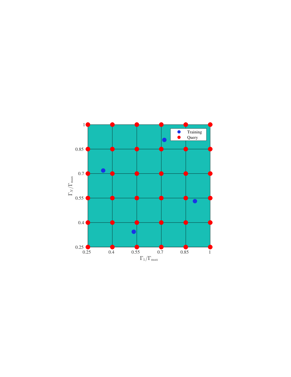
Figure 11 show the parametric experimental results. The time-averaged mean trajectory absolute error, normalized by the characteristic length, , has an average value of 0.0136%. The time-averaged Hamiltonian absolute relative error normalized has an average value of %. Results show that the PTROM is capable of predicting FOM QoIs with sub-0.1% error on average.


Results presented by the QoI error surfaces in Fig. 11, are further highlighted by the queried simulation corresponding to parametric values of in Fig. 12. The simulation in Fig. 12 illustrates the PTROM and FOM (not included in training) particle paths and positions, in addition to the FOM velocity field over a grid with a normalization width of . Figure 12 shows the multi-scale nature of the vortex pair simulation, where particles near the particle with strong circulation, i.e. particle and , orbit the strong particles faster than those further away. The PTROM is capable of following the FOM trajectory with high precision and accuracy for particles not in the neighborhood of the particles with strong circulation, i.e. about particles away from or . Particles in the neighborhood of either or seem to deviate from instantaneous position of the FOM as time passes but are still able to generally follow the path outlined by the FOM.

Finally, Fig. 13 illustrates the surface generated by the query grid speed-up factors. It is seen that the speed-up factor is the highest when the PTROM is running at the edge of the query grid corresponding to either one or both vortex pairs having high circulation. The higher speed-up factor at the edge of the parametric grid corresponds to the increase in wall-time of the FOM needing more Newton iterations to converge as the circulations of and increase. As a result, the increase in Newton iterations also corresponds to more pair-wise interactions incurred that scale like . However, because the PTROM performs a hyper-reduced pair-wise interaction, additional iterations due to the stronger circulations do not incur a significant increase in wall-time. Therefore, the significant increase in FOM wall-time near the edge of the parametric grid and relatively low increase in PTROM wall-time incurs a higher speed-up factor than the interior parametric grid. Overall, it is seen that the PTROM is capable of delivering improved wall-time performance when compared to the FOM.

6.3 Mushroom cloud parametric experiment
The PTROM is now tested against a parametric numerical experiment where two vortices, each with variable circulation and opposing circulation direction, form a mushroom cloud generated with the Biot–Savart law by assigning high variable circulations to end particles and fixed weak circulations to the remaining particles, as was done in the previous experiment. In this experiment, are the input parameters and are part of the parametric space , where . All other particles are assigned a circulation strength of , where and again particles in this experiment. In addition, an inflow condition with a semi-circle profile is added to each particle according to its position on the inflow profile. The inflow profile, , where and , where is a linear distribution from -1 to 1 with increments that are assigned to each particle. The initial positions of the particles follow a linear distribution in the component but have a fixed position in component. The starting positions of the end particles are then and ending . Particles have an initial spacing of 0.15 between each other and the Biot–Savart kernel is assigned a de-singularization cut-off radius equal to the initial spacing distance of 0.15. All simulations were performed in the time interval with leading to time-steps.
The PTROM models were trained at four points in the parametric space denoted by the blue points shown in the grid in Fig. 14. The training points were chosen via the latin hyper-cube sampling method and thirty-six online points were queried online with the PTROM over a grid, where the queried points are denoted by the red points in Fig. 14. All PTROM models in the current experiment were constructed with the following hyper-parameters: and , which results in . Here, the Gauss-Newton relative residual error tolerance was set to tol .
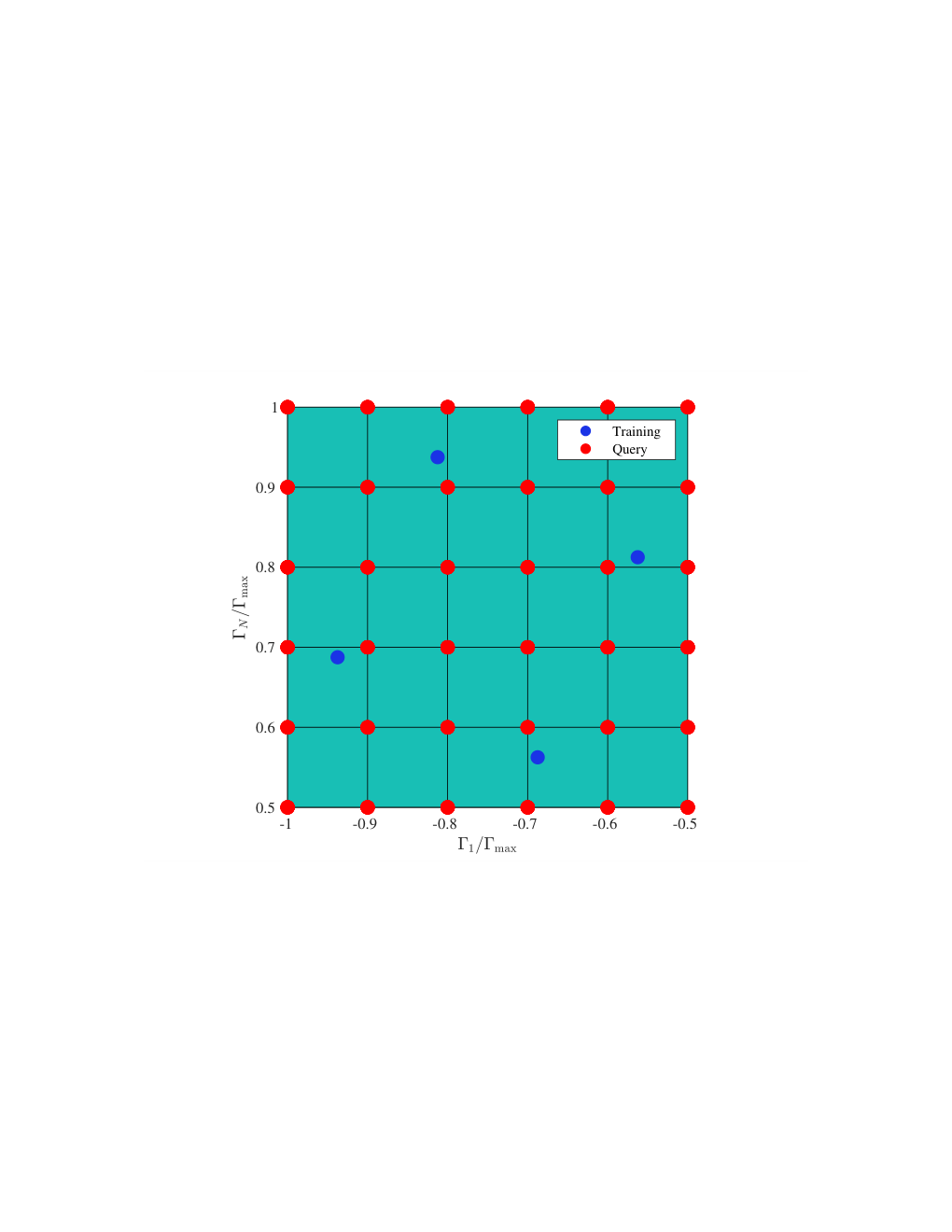
Figure 15 show the parametric experimental results. The time-averaged mean trajectory absolute error, normalized by the characteristic length, , has an average value of 0.0634%. The time-averaged Hamiltonian absolute relative error normalized has an average value of %. Results show that the PTROM is capable of predicting FOM QoIs with sub-0.1% error on average.


Results presented by the QoI error surfaces in Fig. 15, are further highlighted by the queried simulation corresponding to parametric values of in Fig. 16. The simulation in Fig. 16 illustrates the PTROM and FOM (not included in training) particle paths and positions, in addition to the FOM velocity field over a grid with a normalization width of . Figure 16 shows the multi-scale nature of the vortex pair simulation, where particles near the particle with strong circulation, i.e. particle and , orbit the strong particles faster than those further away. Overall the PTROM exhibits similar performance as in the previous experiment with the vortex pair: the PTROM is capable of following the FOM trajectory with high precision and accuracy for particles not in the neighborhood of the particles with strong circulation, i.e. about particles away from or . Particles in the neighborhood of either or seem to deviate from instantaneous position of the FOM as time passes but are still able to generally follow the path outlined by the FOM.

Finally, Fig. 17 illustrates the surface generated by the query grid speed-up factors. As in the prior experiment with the vortex pair, it is seen that the speed-up factor is the highest when the PTROM is running at the edge of the query grid, which corresponds to either one or both vortex pairs having high circulation. The higher speed-up factor at the edge of the parametric grid corresponds to the same reasons as in the previous vortex pair experiment: the increase in wall-time of the FOM is a result of an increase in Newton iterations and pair-wise computations required to converge, which is due to an increase in end-particle circulations. However, because the PTROM performs a hyper-reduced pair-wise interaction, where additional Gauss-Newton iterations do not incur a significant increase in wall-time, additional iterations due to the stronger circulations do not incur a significant increase in wall-time. Therefore, the significant increase in FOM wall-time near the edge of the parametric grid and relatively low increase in PTROM wall-time incurs a higher speed-up factor than the interior parametric grid. Overall, it is seen that the PTROM is capable of delivering improved wall-time performance when compared to the FOM.

6.4 Single vortex reproductive experiment
A reproductive experiment was conducted to assess the performance of the PTROM as the numerical domain increases, i.e. as the number of particles increase, and compared its performance against explicit time integration, hierarchical decomposition, and the GNAT method. Specifically, the PTROM run-time performance was compared against the results from the implicit trapezoidal rule equipped with the Barnes-Hut method (both neighbor clustering and Barnes–Hut clustering were tested) and the GNAT method. In addition, the incurred wall-times of the explicit modified Euler integration (Heun’s integration) and modified Euler integration equipped with the Barnes-Hut method (employing neighbor clustering and Barnes-Hut clustering) were compared to the PTROM. Comparing the PTROM run-time performance with the modified Euler’s time integration helps gauge its performance against traditional rapid time-integrators, such as explicit schemes. Next, QoI reproduction errors as functions of hyper-parameter variation are assessed against incurred wall-times. In other words, Perato fronts for the reproductive experiment are constructed based on QoI error versus wall-time over a range of hyper-parameters. QoIs generated by the explicit integration with and without Barnes–Hut hierarchical decomposition were not compared against the implicit FOM, as it would be inconsistent to measure QoI results of an explicit integration scheme against the implicit FOM QoIs and corresponding GNAT and PTROM results trained by the implicit FOM.
The current reproductive experiment was performed on a range of particle numbers with varying conditions of single vortex simulation that are show in Table 1. The initial positions of particles for all cases listed in Table 1 were defined by a linear distribution in space, i.e. linspace(-N,N,N) in MATLAB syntax, such that the end particles are located at and . The initial distance between each particle was defined by the aforementioned linear distribution of the particle initial positions, and the de-singularization cutoff was set to .
Note: A reproductive experiment and not a parametric experiment was performed to avoid expensive singular value decomposition computations and hierarchical data structures on MATLAB that would completely allocate the random access memory on the machine employed in this investigation. Future work will perform larger scale parametric experiments on a more efficient lower-level language.
| 100 | 500 | 1000 | 2000 | 3000 | 4000 | 5000 | |
|---|---|---|---|---|---|---|---|
| 0.01 | |||||||
| 500 | |||||||
| [0, 20] | [0, 5] | [0, 0.5] | [0, 0.25] | [0, 0.2] | [0, 0.15] | [0, 0.1] |
6.4.1 PTROM reproductive results
Hyper-parameter selection for the PTROM experiments was based on varying the rank of the state POD basis and neighborhood width scaling factor . The residual POD basis rank and sampled particle hyper-parameters followed the change of the state POD basis such that and . Variation of the state POD basis was selected based on loosening and tightening the relative residual tolerances and adjusting the rank of the POD basis enough to satisfy the max iteration criteria of . A discussion is now presented for each hyper-parametric experiment followed by a discussion on the corresponding reproduction errors of QoIs versus wall-times.
Table 2 lists the bases rank variations, , width parameters, , and resulting number of POD source clusters, , for narrow neighborhood widths, i.e. only few neighboring particles have not been clustered. It was found that neighborhood width impacted the rate of convergence of the PTROM and as a result the neighborhood width was widened for and at Bases Case 4 to satisfy the max iteration count criteria for corresponding cases. Future work will look into the underlying reasons of how clustering impacts convergence in the PTROM formulation. It is seen in Table 2 that as the tolerances tighten, additional bases must be added to satisfy the max iteration criteria.
Number of particles, , in the domain tol Hyper-parameter 100 500 1000 2000 3000 4000 5000 Bases Case 1 13 21 21 21 23 23 23 0 0 0 0 0 0 0 68 113 121 122 134 131 142 Bases Case 2 14 22 22 22 23 23 24 0 0 0 0 0 0 0 69 114 129 127 142 130 140 Bases Case 3 14 23 23 23 25 25 26 0 0 0 0 0 0 0 70 120 132 134 136 143 156 Bases Case 4 16 24 24 26 26 26 26 0 0 0 0 0.5 0.5 0.5 80 128 130 134 151 159 144
Figure 18 presents the QoI reproductive results generated by the hyper-parameter settings of Table 2. The time-averaged results shown in Fig. 18(a) illustrate sub 0.1% errors across all cases and particle domain sizes. It is important to point out that as the particle count increases the error decreases, which is due to the PTROM being capable of accurately reproducing the growing number of particle trajectory paths, as reflected in the error quantification via Eq. 30. The time-averaged results shown in Fig. 18(b) also show sub 0.1% errors across all cases and particle domain sizes. Both QoIs errors presented in Fig. 18 reflect an increase in wall-time as the tolerance is tightened. It is interesting to note that for the numerical experiment corresponding to , the QoI errors increase as the tolerance is tightened and more bases are added. It is unknown where this increase in error due to tightened tolerance stems from, but the hypothesis is that narrow neighborhood clustering generates poorer source approximations as more bases are added to the source surrogate POD matrix, , for .
Next, Table 3 lists the bases rank variations, , width parameters, , and resulting number of POD source clusters, , for moderate neighborhood widths, i.e. the number of neighboring particles have increased from the narrow width case and the number of cluster sources have increased. The neighborhood width remained constant through out all hyper-parameter settings, i.e. for all cases. However, it was seen that in the case of for Bases Case 4, the POD basis rank was increased from the prior setting listed in Table 2 to meet the max iteration criteria.
Number of particles, , in the domain tol Hyper-parameter 100 500 1000 2000 3000 4000 5000 Bases Case 1 13 21 21 21 23 23 23 1 1 1 1 1 1 1 73 122 139 123 135 137 149 Bases Case 2 14 22 22 22 23 23 24 1 1 1 1 1 1 1 79 130 142 149 137 150 144 Bases Case 3 14 23 23 23 25 25 26 1 1 1 1 1 1 1 79 127 133 132 146 153 149 Bases Case 4 18 24 24 26 26 26 26 1 1 1 1 1 1 1 84 131 144 144 147 159 143
Figure 19 presents the QoI reproductive results generated by the hyper-parameter settings of Table 3. The time-averaged results shown in Fig. 19(a) illustrate sub 0.1% errors across all cases and particle domain sizes. Similar to results generated by prior hyper-parameter settings in Table 2, as the particle count increases the error decreases, which is due to the PTROM being capable of accurately reproducing the growing number of particle trajectory paths, as reflected in the error quantification via Eq. 30. The time-averaged results shown in Fig. 19(b) also show sub 0.1% errors across all cases and particle domain sizes. Both QoIs errors presented in Fig. 19 reflect an increase in wall-time as the tolerance is tightened and errors decreased. In addition, the increase in neighborhood width has resulted in increased wall-times relative to the hyper-parameter settings for the narrow-width neighborhood settings listed in Table 2.
The final hyper-parametric settings that were tested in this reproductive experiment are presented in Table 4, where the neighborhood width was increased to to increase the number of unclustered neighbors and overall source points. The neighborhood width remained constant through out all hyper-parameter settings, i.e. for all cases. However, it was seen that in Bases Case 4 for and the POD basis rank was increased from the prior setting listed in Table 3 to meet the max iteration criteria. It has been shown so far, with Tables 2 - 4 that hyper-parameter settings impact convergence. Future work will focus on attempting to unveil how the current hyper-parametric settings impact convergence.
Number of particles, , in the domain tol Hyper-parameter 100 500 1000 2000 3000 4000 5000 Bases Case 1 13 21 21 21 23 23 23 2 2 2 2 2 2 2 79 133 135 143 161 183 154 Bases Case 2 14 22 22 22 23 23 24 2 2 2 2 2 2 2 80 130 154 153 164 155 159 Bases Case 3 14 23 23 23 25 25 26 2 2 2 2 2 2 2 80 136 146 165 178 173 173 Bases Case 4 18 24 24 26 26 32 33 2 2 2 2 2 2 2 113 150 143 167 194 216 213
Figure 20 presents the QoI reproductive results generated by the hyper-parameter settings of Table 4. The time-averaged results shown in Fig. 20(a) illustrate sub 0.1% errors across all cases and particle domain sizes. Similar to results generated by prior hyper-parameter settings in Table 3, as the particle count increases the error decreases, which is due to the PTROM being capable of accurately reproducing the growing number of particle trajectory paths, as reflected in the error quantification via Eq. 30. The time-averaged results shown in Fig. 20(b) also show sub 0.1% errors across all cases and particle domain sizes. Both QoIs errors presented in Fig. 20 reflect an increase in wall-time as the tolerance is tightened and errors decreased. In addition, the increase in neighborhood width has resulted in the highest wall-times incurred relative to the hyper-parameter settings for the narrow-width and moderate-width neighborhood settings listed in Table 2 and 3.

6.4.2 GNAT reproductive results
The GNAT method hyper-parameter selection follows the PTROM hyper-parameter settings of Table 2, i.e. the coarsest neighbor-width of the PTROM. However, additional bases were added to the GNAT method if it did not meet the aforementioned max iteration criteria of . Recall that the GNAT method employs no source clustering to the hyper-reduced set of residual computations and computes the influence of all sources. So with this in mind the GNAT method could be thought of as the PTROM method with an infinitely wide neighborhood width, such that there is no clustering of the sources. As a result, only one table of hyper-parameter settings is presented for the GNAT method reproductive experiment in Table 5, where the hyper-parameter settings for the residual POD basis and sampled residuals still hold, i.e. and .
Number of particles, , in the domain tol Hyper-parameter 100 500 1000 2000 3000 4000 5000 Bases Case 1 13 21 21 21 23 23 23 Bases Case 2 14 22 22 22 24 24 25 Bases Case 3 14 24 24 24 25 25 26 Bases Case 4 16 25 25 26 26 26 27
Figure 21 presents the QoI reproductive results generated by the GNAT hyper-parameter settings of Table 5. The time-averaged results shown in Fig. 21(a) illustrate sub 0.1% errors across all cases and particle domain sizes. Similar to results generated by prior PTROM reproductive experiments, as the particle count increases the error decreases due to the GNAT method’s ability to accurately reproduce the growing number of particle trajectory paths. The time-averaged results shown in Fig. 21(b) also show sub 0.1% errors across all cases and particle domain sizes. Both QoIs errors presented in Fig. 21 reflect an increase in wall-time as the tolerance is tightened and errors decreased. It is important to note that the QoI errors generated by the GNAT method are comparable to the PTROM errors, which highlight the minimal impact on QoI accuracy due to source clustering of POD basis in the PTROM method.
6.4.3 Barnes–Hut results
Next, results of the reproductive experiments with traditional hierarchical decomposition via the Barnes–Hut method with Barnes–Hut clustering and neighbor clustering are presented. It is important to note that to generate optimal hierarchical decomposition and clustering results, an additional parametric study was performed on the maximum number of particles contained in each leaf node. Ideally, the optimal choice would be to choose one particle per leaf node as was done in the PTROM. However, the traditional hierarchical decomposition requires online updates and rebuilds of the data-structure. These data-structure rebuilds incur more cost and wall-time if only one particle per leaf node is chosen due to the number of level traversals the algorithm has to go through in its clustering search. The results presented correspond to the simulations that incurred the lowest wall-time in the preliminary hyper-parametric search for the optimal number of particles in each leaf node. Results of this preliminary study are presented in Appendix Acknowledgements. In addition, the number of source clusters is not fixed as it was for the PTROM due to the data-structure updates online and the number of clusters varies per target. As a result the number of clusters are not reported per each hyper-parameter setting for the hierarchical decomposition results.
First, hyper-parameters of the Barnes–Hut hierarchical decomposition with Barnes–Hut clustering are presented in Table 6. Here, generates the lowest number of clusters sources and provides the largest number of cluster sources. Note that if the original FOM would be retrieved.
Number of particles, , in the domain Hyper-parameter 100 500 1000 2000 3000 4000 5000 Barnes–Hut Case 1 2 2 2 2 2 2 2 Barnes–Hut Case 2 1 1 1 1 1 1 1 Barnes–Hut Case 3 0.5 0.5 0.5 0.5 0.5 0.5 0.5
Figure 22 presents the QoI reproductive results generated by the Barnes–Hut hyper-parameter settings listed in Table 6. The time-averaged results shown in Fig. 22(a) illustrate improved reproductive errors, with respect to both PTROM and GNAT methods, that are all sub 0.001% errors across all cases and particle domain sizes. Similar to results generated by prior PTROM and GNAT reproductive experiments, as the particle count increases the error decreases due to the hierarchical decomposition method’s ability to accurately reproduce the growing number of particle trajectory paths. The time-averaged results shown in Fig. 22(b) also show an improved error over PTROM and GNAT method with sub 0.001% error across all cases and particle domain sizes. The hierarchical decomposition method even reaches errors down to . However, it is important to note that the decrease in errors come with an increased wall-time of about two orders of magnitude with respect to the PTROM results in Fig. 18. A more detailed discussion of wall-time time performance across all methods will be given in Section 6.4.4
Next, hyper-parameters of the Barnes–Hut hierarchical decomposition with neighbor search clustering are presented in Table 7. Here, generates the lowest number of clusters sources and generates the largest number of cluster sources. Note that as the original FOM would be retrieved.
Number of particles, , in the domain Hyper-parameter 100 500 1000 2000 3000 4000 5000 Nearest-Neighbor Case 1 0 0 0 0 0 0 0 Nearest-Neighbor Case 2 1 1 1 1 1 1 1 Nearest-Neighbor Case 3 2 2 2 2 2 2 2
Figure 23 presents the QoI reproductive results generated by the Barnes–Hut hyper-parameter settings listed in Table 7. The time-averaged results shown in Fig. 23(a) illustrate improved reproductive errors, with respect to both PTROM and GNAT methods, that are all sub 0.01% errors across all cases and particle domain sizes. Similar to results generated by prior PTROM and GNAT reproductive experiments, as the particle count increases the error decreases due to the hierarchical decomposition method’s ability to accurately reproduce the growing number of particle trajectory paths. The time-averaged results shown in Fig. 23(b) also show an improved error over PTROM and GNAT method with sub 0.01% error across all cases and particle domain sizes. The hierarchical decomposition method even reaches errors down to . However, it is important to note that the decrease in errors come with an increased wall-time of about two orders of magnitude with respect to the PTROM results in Fig. 18. A more detailed discussion of wall-time time performance across all methods will is now given.
6.4.4 Computational savings and performance
Wall-time and corresponding speed-up of the PTROM are presented in Fig. 24. Specifically, the PTROM narrow-width bases case 1 (highest PTROM computational savings) and narrow-width bases case 4 (lowest PTROM computational savings) are compared against GNAT bases case 1 and 4, and against the Barnes–Hut hierarchical decomposition with Barnes–Hut clustering set to and neighbor search clustering with . In addition, the FOM with an explicit predictor-corrector modified Euler time integration is compared with the PTROM. Finally, the modified Euler’s technique is equipped with hiearchical decomposition is also compared, such that Barnes–Hut clustering is set to and neighbor search clustering is set to .
From an overhead view, results presented in Fig. 24 show that the PTROM equipped with narrow-width neighbor search clustering and bases case 1, operates logarithmically efficient and out-performs all time-integration methods as the number of increase. However, at , the GNAT equipped with bases case 1 out-performs the PTROM due to lower number of iterations incurred during the Gauss-Newton loop. However, as the number of particles increases the GNAT cannot out-perform the PTROM even if less Gauss-Newton iterations are incurred, as the GNAT pair-wise interaction loop requires back-projection from the low-dimensional embedding back to the high-dimensional space to perform summation over all at the sampled residuals. Recall, the PTROM hyper-reduced pair-wise interaction does not require back-projection or summation over all sources. Similarly, at and the explicit hierarchical decomposition out-performs the PTROM method with wide-width neighbor search clustering and Bases Case 4, which can be attributed to the rapid explicit nature of the time integration which requires no Newton iterations. However, as the number of particles increases the explicit time-integration cannot out-perform the PTROM method even with a tight tolerance and relatively conservative hyper-parameters, i.e. Bases Case 4 with wide-width neighbor search clustering.
Figure 24(b) highlights the computational performances of the implicit hierarchical decomposition, GNAT, and PTROM methods in terms of a speed-up factor as presented in Eq. 31. It is shown in Fig. 24(b) that the PTROM can reach a speed-up factor of up to 2199, i.e. the PTROM can generate results over 2000 times faster than the FOM and deliver sub 0.1 % QoI reproductive erros for . The GNAT performance for Bases Case 1 provides a speed-up factor of 678 for . Barnes–Hut and narrow-neighbor search clustering for the hierarchical decomposition approach can at best provide a speed-up factor of 8.68 and 5.35 respectively.
Figures 25 and 26 provide qualitative results of the PTROM for using Bases Case 1 for a narrow-width neighbor search and Bases Case 4 for a wide-width neighbor search, respectively. Results show that the PTROM is capable of reproducing the FOM particle trajectories to a high level of accuracy away from the center particle with strong circulation. In the case of the PTROM with hyper-parameter settings of Bases Case 1 and a narrow-width neighbor search, results show a deviation in particle path trajectory near the center particle where the particle velocities increase inversely proportional to the squared distance from the center particle, as quantified by the Biot-Savart law in Eq. 2. However, in the case of the PTROM with Bases Case 4 for a wide-width neighbor search, the additional bases and sources along with a tightened tolerance has significantly improved the trajectory reconstruction near the center particle.


7 Conclusions
In this work, the projection-tree reduced order modeling (PTROM) technique is presented. The PTROM provides a new perspective in accelerating -body problems by bridging traditional hierarchical decomposition methods with recent advancements in projection-based reduced order modeling to overcome the pairwise interaction problem and achieve -independent operational count complexity. The PTROM is based on performing projection-based model reduction via the Gauss–Newton with approximated tensors (GNAT) approach, and hierarchical decomposition via the Barnes–Hut tree method. The effectiveness of the PTROM was tested on parametric and reproductive problems. In the parametric experiments, the PTROM was tested on vortex simulations with 1000 degrees-of-freedom where variable vortex circulation over a predefined space corresponded to parametric inputs. It was shown that the PTROM can deliver on average QoI errors between 0.0135-0.0634% while delivering 1.7-3.94 computational speed-up, all with respect to the FOM. In the reproductive experiments, the PTROM was tested on a vortex simulation with degrees-of-freedom ranging from 200 to 10000 and was compared against stand-alone hiearchical decomposition methods, stand-alone projection-based model reduction, and explicit time integration with and without hierarchical decomposition. A range of PTROM hyper-parameters were varied and it was found that the PTROM was capable of delivering sub-0.1% errors while delivering over a 2000 speed-up and out-performed explicit integration, the GNAT method, Barnes-Hut hierarchical decomposition with implicit and explicit integration.
Future work will involve investigating the impact hyper-parameters have on the PTROM convergence, and performing parallelized simulations with a large-scale particle count to assess more rigorously computional savings, core-hours, and resource expense. In addition, future work will include equipping the PTROM with more recent advances in model-reduction that include integrating nonlinear manifolds discovered by convolutional neural networks as the underlying reduced basis for dimensional compression. Future work will also focus on more physics driven applications of the PTROM, such as modeling heat-deposition of additive manufacturing, and heat/fluid transport phenomena.
Acknowledgements
The inception of this work was developed while S. N. Rodriguez held a visiting scientist position at the University of Washington, Seattle. S. N. Rodriguez would like to acknowledge the NRL Isabella and Jerome Karle’s Distinguished Scholar Fellowship and Dr. Nathan F. Wagenhoffer for his expertise and insightful conversations on hierarchical decomposition and -body acceleration methods. S. L. Brunton would like to acknowledge support from the ARO PECASE (W911NF-19-1-0045). A. P. Iliopoulos, J. C. Steuben, and J. G. Michopoulos would like to acknowledge support from ONR through NRL core funding.
Appendix A Barnes–Hut search for maximum particles per leaf node
As discussed in Section 6.4.3, an additional parametric study was performed to find the maximum number of points per leaf nodes that would provide the most rapid results given the clustering hyper-parameters chosen in Tables 6 and 7. The maximum number of particles per leaf node (MMPL) were chosen by running the hyper-parameters in Tables 6 and 7 for a range of points per leaf node and chose the simulation with the lowest wall-time to compare against the PTROM. Results for the hierarchical decomposition with implicit time integration are presented in Fig. 27 and Fig. 28.
It was found that hierarchical decomposition did not improve pairwise interaction computations for lower particle count since the data structure build would incur more cost than computing the simulations directly. As a result the fastest run time for some particle counts were those that had the maximum number of particles per leaf node equal to the total number of particles in the domain. Tables 8 and 9 list the maximum number of points chosen for each clustering hyper-parameter and in the implicit and explicit integration cases, respectively.
Barnes–Hut clustering MPPL Neighbor search clustering MPPL 100 100 100 100 100 100 100 500 500 50 50 100 500 500 1000 1000 75 50 100 75 75 2000 100 100 100 100 50 50 3000 75 75 75 75 75 75 4000 100 100 100 100 100 40 5000 125 125 125 125 50 50
Barnes–Hut clustering MPPL Neighbor search clustering MPPL 100 100 100 100 100 100 100 500 500 38 50 50 50 450 1000 100 75 50 50 50 50 2000 50 100 100 100 100 50 3000 75 75 75 75 75 75 4000 100 100 100 100 100 40 5000 50 125 125 125 125 50
References
- Afkham and Hesthaven [2017] Afkham, B.M., Hesthaven, J.S., 2017. Structure preserving model reduction of parametric Hamiltonian systems. SIAM Journal on Scientific Computing 39, A2616–A2644.
- Akoz and Moored [2018] Akoz, E., Moored, K.W., 2018. Unsteady propulsion by an intermittent swimming gait. Journal of Fluid Mechanics 834, 149.
- Amsallem and Farhat [2012] Amsallem, D., Farhat, C., 2012. Stabilization of projection-based reduced-order models. International Journal for Numerical Methods in Engineering 91, 358–377.
- Amsallem et al. [2012] Amsallem, D., Zahr, M.J., Farhat, C., 2012. Nonlinear model order reduction based on local reduced-order bases. International Journal for Numerical Methods in Engineering 92, 891–916.
- Antoulas [2005] Antoulas, A.C., 2005. Approximation of large-scale dynamical systems. SIAM.
- Barnes and Hut [1986] Barnes, J., Hut, P., 1986. A hierarchical o (n log n) force-calculation algorithm. nature 324, 446.
- Barrault et al. [2004] Barrault, M., Maday, Y., Nguyen, N.C., Patera, A.T., 2004. An ‘empirical interpolation’method: application to efficient reduced-basis discretization of partial differential equations. Comptes Rendus Mathematique 339, 667–672.
- Benner et al. [2017] Benner, P., Ohlberger, M., Cohen, A., Willcox, K., 2017. Model reduction and approximation: theory and algorithms. SIAM.
- Brown and Line [2005] Brown, R.E., Line, A.J., 2005. Efficient high-resolution wake modeling using the vorticity transport equation. AIAA journal 43, 1434–1443.
- Brunton and Kutz [2019] Brunton, S.L., Kutz, J.N., 2019. Data-driven science and engineering: Machine learning, dynamical systems, and control. Cambridge University Press.
- Brunton and Noack [2015] Brunton, S.L., Noack, B.R., 2015. Closed-loop turbulence control: Progress and challenges. Applied Mechanics Reviews 67.
- Buffa et al. [2012] Buffa, A., Maday, Y., Patera, A.T., Prud’homme, C., Turinici, G., 2012. A priori convergence of the greedy algorithm for the parametrized reduced basis method. ESAIM: Mathematical Modelling and Numerical Analysis-Modélisation Mathématique et Analyse Numérique 46, 595–603.
- Bui-Thanh et al. [2008] Bui-Thanh, T., Willcox, K., Ghattas, O., 2008. Model reduction for large-scale systems with high-dimensional parametric input space. SIAM Journal on Scientific Computing 30, 3270–3288.
- Carlberg et al. [2017] Carlberg, K., Barone, M., Antil, H., 2017. Galerkin v. least-squares Petrov–Galerkin projection in nonlinear model reduction. Journal of Computational Physics 330, 693–734.
- Carlberg et al. [2015] Carlberg, K., Tuminaro, R., Boggs, P., 2015. Preserving Lagrangian structure in nonlinear model reduction with application to structural dynamics. SIAM Journal on Scientific Computing 37, B153–B184.
- Carlberg et al. [2013] Carlberg, K.T., Farhat, C., Cortial, J., Amsallem, D., 2013. The GNAT method for nonlinear model reduction: effective implementation and application to computational fluid dynamics and turbulent flows. Journal of Computational Physics 242, 623–647.
- Chaturantabut and Sorensen [2010] Chaturantabut, S., Sorensen, D.C., 2010. Nonlinear model reduction via discrete empirical interpolation. SIAM Journal on Scientific Computing 32, 2737–2764.
- Cipra [2000] Cipra, B.A., 2000. The best of the 20th century: Editors name top 10 algorithms. SIAM news 33, 1–2.
- Colmenares et al. [2015] Colmenares, J.D., López, O.D., Preidikman, S., 2015. Computational study of a transverse rotor aircraft in hover using the unsteady vortex lattice method. Mathematical Problems in Engineering 2015.
- Doerr et al. [2016] Doerr, S., Harvey, M., Noé, F., De Fabritiis, G., 2016. Htmd: high-throughput molecular dynamics for molecular discovery. Journal of chemical theory and computation 12, 1845–1852.
- Dongarra and Sullivan [2000] Dongarra, J., Sullivan, F., 2000. Guest editors’ introduction: The top 10 algorithms. Computing in Science & Engineering 2, 22.
- Eldredge [2007] Eldredge, J.D., 2007. Numerical simulation of the fluid dynamics of 2d rigid body motion with the vortex particle method. Journal of Computational Physics 221, 626–648.
- Eldredge et al. [2002] Eldredge, J.D., Colonius, T., Leonard, A., 2002. A vortex particle method for two-dimensional compressible flow. Journal of Computational Physics 179, 371–399.
- Erichson et al. [2019] Erichson, N.B., Mathelin, L., Kutz, J.N., Brunton, S.L., 2019. Randomized dynamic mode decomposition. SIAM Journal on Applied Dynamical Systems 18, 1867–1891.
- Everson and Sirovich [1995] Everson, R., Sirovich, L., 1995. Karhunen–Loeve procedure for gappy data. JOSA A 12, 1657–1664.
- Farhat et al. [2014] Farhat, C., Avery, P., Chapman, T.and Cortial, J., 2014. Dimensional reduction of nonlinear finite element dynamic models with finite rotations and energy-based mesh sampling and weighting for computational efficiency. International Journal for Numerical Methods in Engineering 98, 625–662.
- Farhat et al. [2015] Farhat, C., Chapman, T., Avery, P., 2015. Structure-preserving, stability, and accuracy properties of the energy-conserving sampling and weighting method for the hyper reduction of nonlinear finite element dynamic models. International Journal for Numerical Methods in Engineering 102, 1077–1110.
- Gaertner and Lackner [2015] Gaertner, E.M., Lackner, M.A., 2015. Modeling dynamic stall for a free vortex wake model. Wind Engineering 39, 675–691.
- Gnedin [2019] Gnedin, N.Y., 2019. Hierarchical particle mesh: An FFT-accelerated fast multipole method. The Astrophysical Journal Supplement Series 243, 19.
- Greengard and Rokhlin [1987] Greengard, L., Rokhlin, V., 1987. A fast algorithm for particle simulations. Journal of Computational Physics 73, 325–348.
- Grepl et al. [2007] Grepl, M.A., Maday, Y., Nguyen, N.C., Patera, A.T., 2007. Efficient reduced-basis treatment of nonaffine and nonlinear partial differential equations. ESAIM: Mathematical Modelling and Numerical Analysis 41, 575–605.
- Guo and Hesthaven [2019] Guo, M., Hesthaven, J.S., 2019. Data-driven reduced order modeling for time-dependent problems. Computer methods in applied mechanics and engineering 345, 75–99.
- Hansson et al. [2002] Hansson, T., Oostenbrink, C., van Gunsteren, W.F., 2002. Molecular dynamics simulations. Current opinion in structural biology 12, 190–196.
- Holmes et al. [2012] Holmes, P., Lumley, J.L., Berkooz, G., Rowley, C.W., 2012. Turbulence, coherent structures, dynamical systems and symmetry. Cambridge university press.
- Jeon et al. [2014] Jeon, M., Lee, S., Lee, S., 2014. Unsteady aerodynamics of offshore floating wind turbines in platform pitching motion using vortex lattice method. Renewable Energy 65, 207–212.
- Jiang et al. [2016] Jiang, X., Li, J., Zhao, X., Qin, J., Karpeev, D., Hernandez-Ortiz, J., de Pablo, J.J., Heinonen, O., 2016. An and parallel approach to integral problems by a kernel-independent fast multipole method: Application to polarization and magnetization of interacting particles. The Journal of Chemical Physics 145, 064307.
- Jing and Stephansson [2007] Jing, L., Stephansson, O., 2007. Fundamentals of discrete element methods for rock engineering: theory and applications. volume 85. Elsevier.
- Kebbie-Anthony et al. [2018] Kebbie-Anthony, A.B., Gumerov, N., Preidikman, S., Balachandran, B., Azarm, S., 2018. Fast multipole method for nonlinear, unsteady aerodynamic simulations, in: 2018 AIAA Modeling and Simulation Technologies Conference, p. 1929.
- Kutz et al. [2016] Kutz, J.N., Brunton, S.L., Brunton, B.W., Proctor, J.L., 2016. Dynamic mode decomposition: data-driven modeling of complex systems. volume 149. Siam.
- Lee and Carlberg [2020] Lee, K., Carlberg, K.T., 2020. Model reduction of dynamical systems on nonlinear manifolds using deep convolutional autoencoders. Journal of Computational Physics 404, 108973.
- Leishman [2006] Leishman, G.J., 2006. Principles of helicopter aerodynamics with CD extra. Cambridge university press.
- Liu and Liu [2010] Liu, M.B., Liu, G.R., 2010. Smoothed particle hydrodynamics (SPH): an overview and recent developments. Archives of computational methods in engineering 17, 25–76.
- Martinsson [2015] Martinsson, P.G., 2015. Fast Multipole Methods. Springer Berlin Heidelberg, Berlin, Heidelberg. pp. 498–508. URL: https://doi.org/10.1007/978-3-540-70529-1_448, doi:10.1007/978-3-540-70529-1_448.
- Martinsson and Rokhlin [2007] Martinsson, P.G., Rokhlin, V., 2007. An accelerated kernel-independent fast multipole method in one dimension. SIAM Journal on Scientific Computing 29, 1160–1178.
- Mocz and Succi [2015] Mocz, P., Succi, S., 2015. Numerical solution of the nonlinear schrödinger equation using smoothed-particle hydrodynamics. Physical Review E 91, 053304.
- Noack et al. [2016] Noack, B.R., Stankiewicz, W., Morzynski, M., Schmid, P.J., 2016. Recursive dynamic mode decomposition of transient and post-transient wake flows. Journal of Fluid Mechanics 809, 843.
- Nocedal and Wright [2006] Nocedal, J., Wright, S., 2006. Numerical optimization. Springer Science & Business Media.
- Noé and Clementi [2015] Noé, F., Clementi, C., 2015. Kinetic distance and kinetic maps from molecular dynamics simulation. Journal of Chemical Theory and Computation 11, 5002–5011.
- Parish and Carlberg [2020] Parish, E.J., Carlberg, K.T., 2020. Time-series machine-learning error models for approximate solutions to parameterized dynamical systems. Computer Methods in Applied Mechanics and Engineering 365, 112990.
- Peng and Mohseni [2016] Peng, L., Mohseni, K., 2016. Symplectic model reduction of Hamiltonian systems. SIAM Journal on Scientific Computing 38, A1–A27.
- Pfalzner and Gibbon [2005] Pfalzner, S., Gibbon, P., 2005. Many-body tree methods in physics. Cambridge University Press.
- Pfrommer et al. [2006] Pfrommer, C., Springel, V., Enßlin, T.A., Jubelgas, M., 2006. Detecting shock waves in cosmological smoothed particle hydrodynamics simulations. Monthly Notices of the Royal Astronomical Society 367, 113–131.
- Rodriguez [2018] Rodriguez, S.N., 2018. Stability and Dynamic Properties of Tip Vortices Shed from Flexible Rotors of Floating Offshore Wind Turbines. Ph.D. thesis. Lehigh University.
- Rodriguez et al. [2020a] Rodriguez, S.N., Iliopoulos, A.P., Michopoulos, J.G., Jaworski, J.W., 2020a. Investigating the coupled effects between rotor-blade aeroelasticity and tip vortex stability, in: International Design Engineering Technical Conferences and Computers and Information in Engineering Conference, American Society of Mechanical Engineers. p. V009T09A001.
- Rodriguez and Jaworski [2017] Rodriguez, S.N., Jaworski, J.W., 2017. Toward identifying aeroelastic mechanisms in near-wake instabilities of floating offshore wind turbines. Journal of Energy Resources Technology, Special Issue: Wind Energy 139, 051203.
- Rodriguez and Jaworski [2019] Rodriguez, S.N., Jaworski, J.W., 2019. Strongly-coupled aeroelastic free-vortex wake framework for floating offshore wind turbine rotors. part 1: Numerical framework. Renewable Energy 141, 1127–1145.
- Rodriguez and Jaworski [2020] Rodriguez, S.N., Jaworski, J.W., 2020. Strongly-coupled aeroelastic free-vortex wake framework for floating offshore wind turbine rotors. part 2: Application. Renewable Energy 149, 1018–1031.
- Rodriguez et al. [2020b] Rodriguez, S.N., Jaworski, J.W., Michopoulos, J.G., 2020b. Stability of helical vortex structures shed from flexible rotors. arXiv preprint arXiv:2008.08969 .
- Rowley [2005] Rowley, C.W., 2005. Model reduction for fluids, using balanced proper orthogonal decomposition. International Journal of Bifurcation and Chaos 15, 997–1013.
- Rowley et al. [2004] Rowley, C.W., Colonius, T., Murray, R.M., 2004. Model reduction for compressible flows using POD and Galerkin projection. Physica D: Nonlinear Phenomena 189, 115–129.
- Russell et al. [2018] Russell, M.A., Souto-Iglesias, A., Zohdi, T., 2018. Numerical simulation of laser fusion additive manufacturing processes using the sph method. Computer Methods in Applied Mechanics and Engineering 341, 163–187.
- Schmid [2010] Schmid, P.J., 2010. Dynamic mode decomposition of numerical and experimental data. Journal of fluid mechanics 656, 5–28.
- Sebastian and Lackner [2012] Sebastian, T., Lackner, M., 2012. Development of a free vortex wake method code for offshore floating wind turbines. Renewable Energy 46, 269–275.
- Shadloo et al. [2016] Shadloo, M.S., Oger, G., Le Touzé, D., 2016. Smoothed particle hydrodynamics method for fluid flows, towards industrial applications: Motivations, current state, and challenges. Computers & Fluids 136, 11–34.
- Sirovich [1987] Sirovich, L., 1987. Turbulence and the dynamics of coherent structures. i. coherent structures. Quarterly of applied mathematics 45, 561–571.
- Steuben et al. [2016] Steuben, J.C., Iliopoulos, A.P., Michopoulos, J.G., 2016. Discrete element modeling of particle-based additive manufacturing processes. Computer Methods in Applied Mechanics and Engineering 305, 537–561.
- Taira et al. [2017] Taira, K., Brunton, S.L., Dawson, S.T.M., Rowley, C.W., Colonius, T., McKeon, B.J., Schmidt, O.T., Gordeyev, S., Theofilis, V., Ukeiley, L.S., 2017. Modal analysis of fluid flows: An overview. Aiaa Journal 55, 4013–4041.
- Tartakovsky and Meakin [2005] Tartakovsky, A.M., Meakin, P., 2005. A smoothed particle hydrodynamics model for miscible flow in three-dimensional fractures and the two-dimensional rayleigh–taylor instability. Journal of Computational Physics 207, 610–624.
- Tiso and Rixen [2013] Tiso, P., Rixen, D.J., 2013. Discrete empirical interpolation method for finite element structural dynamics, in: Topics in Nonlinear Dynamics, Volume 1. Springer, pp. 203–212.
- Tu et al. [2013] Tu, J.H., Rowley, C.W., Luchtenburg, D.M., Brunton, S.L., Kutz, J.N., 2013. On dynamic mode decomposition: theory and applications. Journal of Nonlinear Science 22, 887–915.
- Wang et al. [2019] Wang, J., Olsson, S., Wehmeyer, C., Pérez, A., Charron, N.E., De Fabritiis, G., Noé, F., Clementi, C., 2019. Machine learning of coarse-grained molecular dynamics force fields. ACS central science 5, 755–767.
- Willcox and Peraire [2002] Willcox, K., Peraire, J., 2002. Balanced model reduction via the proper orthogonal decomposition. AIAA journal 40, 2323–2330.
- Ying [2006] Ying, L., 2006. A kernel independent fast multipole algorithm for radial basis functions. Journal of Computational Physics 213, 451–457.
- Ying et al. [2004] Ying, L., Biros, G., Zorin, D., 2004. A kernel-independent adaptive fast multipole algorithm in two and three dimensions. Journal of Computational Physics 196, 591–626.