Audio scene monitoring using redundant un-localized microphone arrays
Abstract
We present a system for localizing sound sources in a room with several microphone arrays. Unlike most existing approaches, the positions of the arrays in space are assumed to be unknown. Each circular array performs direction of arrival (DOA) estimation independently. The DOAs are then fed to a fusion center where they are concatenated and used to perform the localization based on two proposed methods, which require only few labeled source locations for calibration. The first proposed method is based on principal component analysis (PCA) of the observed DOA and does not require any calibration. The array cluster can then perform localization on a manifold defined by the PCA of concatenated DOAs over time. The second proposed method performs localization using an affine transformation between the DOA vectors and the room manifold. The PCA approach has fewer requirements on the training sequence, but is less robust to missing DOAs from one of the arrays. The approach is demonstrated with a set of five 8-microphone circular arrays, placed at unknown fixed locations in an office. Both the PCA approach and the direct approach can easily map out a rectangle based on a few calibration points with similar accuracy as calibration points. The methods demonstrated here provide a step towards monitoring activities in a smart home and require little installation effort as the array locations are not needed.
August 11, 2026
Index Terms:
Smart homes, circular microphone arrays, sound localization, self-calibration.I Introduction
Microphone arrays, in the form of smart speakers, have become an affordable household item. As a result, these systems are ubiquitous, and there may be many microphone arrays in a single room. Most audio array systems require knowledge of the relative locations and orientations of the arrays. We instead use a few source calibration points with known relative locations, which are easier to implement. By using redundant arrays, we obtain higher accuracy and are less concerned with array placement.
In this paper we describe localization approaches which use several microphone arrays of unknown locations. The DOAs from each array are then collected through WiFi to a central fusion center where they are concatenated to form a global DOA vector. Based on the global DOA vector we perform localization in a room with two proposed methods: a subspace method based on PCA and an affine mapping-based approach.
We first consider localization using principal component analysis (PCA) to obtain a low-dimensional mapping of the DOA vector observations over time and space. This PCA approach does not require knowledge of calibration source location, just an association between PCA coordinates and room coordinates. The mapping requires the relative location of calibration points, say corner of a table. While this approach does not provide physical dimensions, it can give relations between locations in a room.
We also consider a localization approach based on affine mapping between the DOA vector and room coordinates. This mapping is more robust to missing array DOAs than the PCA approach, as it is based on a physical mapping to room coordinates. To train the mapping it also requires relative location of calibration points.
For our experiments, we have five arrays, placed at fixed unknown locations in a reverberant office environment. The arrays are connected to a Raspberry Pi 3, which runs the Open embeddeD Audition System (ODAS) software, [1, 2] and can track the directions of arrival (DOAs) for up to four sound sources simultaneously. This open-source framework is appealing as it allows on-board DOA estimation for each microphone array. We use this existing system to observe the sound sources and compute their DOA relative to the array.
Such a setup could be useful for improving monitoring of sound events in a smart home, using existing arrays [3]. Since the DOA processing is performed on-board, this helps preserve privacy, as audio in this approach is not share over the network. This could be used for fall monitoring [4] and daily events classification [5]. This system could also be combined to sound scene classification, e.g., [6, 7].
I-A Related work
Alternative methods would combine the whole array stream of data at the fusion center by using maximum likelihood beamforming for multiple arrays [8, 9] and localize the arrays in an ad hoc network [10]. In our approach, where the DOAs are processed at the individual arrays, we benefit from transmitting just the DOA stream. This requires less bandwidth than using the raw array output. In terms of privacy this is a huge improvement as no signals are transmitted to the fusion center. In a fusion center multiple DOAs can be used for localization based on known array positions[11].
Resolving closely spaced acoustic sources when the noise power is varying in space and time has been studied extensively. As part of ODAS, we rely on the low-complexity Steered-Response Power Phase Transform (SRP-PHAT) to estimate DOAs [12, 1]. Many other methods could be used such as adaptive beamformers [13] or compressive DOA estimation [14, 15, 16, 17]. Sparse Bayesian learning (SBL) [15, 18, 19, 20, 21] could also be used. Multiple Signal Classification (MUSIC) [22] is also common for localization in noisy environments [23, 24]. DOA estimation could also rely on machine leaning [25, 26]. Since each circular array has well-defined geometry classical array processing seems more appropriate, and machine learning could be used in the combination of the arrays. More features than just DOA could be beneficial for localization [27], e.g., echoes [28]. As a low-complexity approach, just three microphones have been used [29].
In the future, more advanced machine learning (ML)[30] could help with this task as it already did in related localization problems. In particular, ML approaches might better-address the inherent non-linearity in sound localization. Neural network classifier [31, 32, 25, 33] or semi supervised learning[34, 35, 36] would be of first interest.
Many indoor localization systems have been proposed [37]. Sound source localization (SSL) also has widespread applications in human-robot interaction [38], ocean acoustics [39], teleconferencing [40], drone localization [41], and automatic speech recognition [42]. These have been designed for various applications as indoor navigation, communication and health. In general, they involve a first step where receiver geometric configuration such as distances and angles are measured. In the second step, the target is located using the measured data. Our proposed system replaces the first step with a training/calibration step.
DOAs are the only features used here. Other systems also use travel time difference of arrival between the arrays [43]. This requires a precise relative clock for each array system, maybe requiring more hardware. The actual system implemented here cost about 200 USD for one array. The proposed system is demonstrated with active sources at well-known points. This serves to better validate the approach.

II Processing localization
We assume a room equipped with time-synchronized circular microphone arrays, which provides the DOAs based on a local coordinate system. The DOA for each array lies on a virtual unit half-sphere in the positive -plane (see Fig. 1), and is defined as , where and . Our development and processing use the output DOA vectors of the time-synchronized arrays as they arrive at the fusion center.
From the M arrays we obtain one dimensional DOA vector from one sound source. The array positions are unknown. Thus, to perform source localization we first need to do training based on previous observations of the vector, collected into a matrix , called calibration DOAs. We propose two methods:
Sec. II-A method relies on observing and then performing principal component analysis (PCA) on this matrix. Thus, we localize the source in a PCA space. The location of the sources generating the matrix can be unknown.
Sec. II-B–II-D approach assumes an affine transformation between dimensional -vector and the local dimensional room.
For the first approach we need all (or the same) arrays observing the sound source of interest, but no calibration sources are needed. For the second approach we need a set of calibration sources (more than 3).
II-A PCA
Performing PCA on the observed DOA vectors gives , with the left and right singular vectors and the singular values. Assuming the relation between DOA and spatial location is approximately linear (3) with N (2 or 3) spatial coordinates, the first (2 or 3) singular DOA vectors should be sufficient to describe the location. Throughout the rest of the paper, we use first components, as all sources are mainly in the 2-D horizontal plane.
Decomposing the th DOA observation with only the first singular vectors used, the reduced .
| (1) |
where are the coefficients of the two singular vectors that define the DOA vector . Since physically there should only be 2–3 large components, finding the decomposition in PCA space defines an unknown room position.
In the above processing, it is assumed that all arrays observe all the sources. However, in a real system there will always be missing observations due to malfunctioning arrays, nature of the room setup, source directivity or weak sources. This can happen in either the calibration or the mapping part of the experiments.
For mapping to PCA coordinates, omitting the missing array is easy, but the sound source will then map to a different location in PCA space. Thus, for sources evolving sequentially in time it is preferred to only use the arrays that is continuously tracking the source.
II-B Affine mapping to room manifold
In general, the mapping between -dimensional room observations ( is 2 or 3) and -dimensional DOA vector is non-linear and unknown
| (2) |
The non-linear variation of the DOA vector vs spatial location for one array is indicated in Fig. 2. We assume a linear mapping (affine transformation) might be sufficient for this mapping of a room. This was observed to work well for the DOA variation in the room used here, see Sec. IV. The affine transformation is
| (3) |
where is the offset and are the linear coefficients. Both and are determined in Sec. II-C by performing recording at locations .
Typically, a weak source is not observed on all arrays, giving a DOA observation with non-active elements, we then retain the active elements in produced by the list of active arrays . From the calibration DOA matrix we only use the active arrays . For each DOA observation and , we then determine the function with only the entries of the calibration DOA corresponding to active arrays and use this to determine the matrix for just . This matrix is then multiplied with the active DOAs . The non-active elements are not used in the mapping. This gives
| (4) |
For each case of active DOAs, the matrix is determined as in Sec. II-C.
II-C Linear mapping calibration
We perform a sound source recording at locations, for location we have observations . For all observations, we obtain the matrix of DOA observations generated from a source with corresponding location matrix
| (5) |
where is a vector of length with all ones.
Defining the cost function (using the trance operator Tr and Frobenius norm )
| (6) |
Differentiating the cost function
| (7) | ||||
| (8) | ||||
| (9) |
Forcing (8) to zero gives ( is the mean operator over observations )
| (10) |
Forcing (9) to zero gives
| (11) |
where + denotes the Moore-Penrose pseudo-inverse. Thus, the mapping is determined from (11). The number of calibration points needed depends on the uniqueness of the points in spatial and DOA space. In general, for an -dimensional room space, calibration points spanning the space are sufficient. Using just 2 calibration points maps all observations to a line between the points and 3 calibration point is sufficient spanning a 2D plane.
II-D Disturbances from reference point
For a known reference point between a DOA vector and room location , an approximate mapping from a measurement to a new room location is for a given matrix:
| (12) |
For a given matrix learned though the calibration points, we do the mapping by selecting a reference point close to the observed and use (12).
Similarly, for a known DOA PCA components (as in (1)) and room location and given a PCA observation the new room location is
| (13) |
and describes the mapping from the DOA PCA components to spatial location. From (13) it is clear that there are an approximately a linear relation between PCA space and location.
II-E Unknown calibration source location
The PCA method comes handy when it is impractical to measure the exact positions of sound sources for calibration. Thus, we perform the source experiments with unknown locations and compute the singular vectors from these observations to enable PCA. Then for a new source we perform localization in this PCA space and describe the solution in term of proximity to the sources in PCA space.

a)

b)
III Experimental design
III-A Circular microphone array
We used arrays that are part of development kit called Matrix Creator11 1 https://www.matrix.one/products/creator with software (ODAS22 2 http://odas.io) that computes the DOA using the Steered response power with phase transform (SRP-PHAT)[12, 1] as summarized below as background information.
Each array consists of 8 microphones, uniformly placed in circle with 10 cm diameter, and connected to a Raspberry Pi 3 device33 3 https://www.raspberrypi.org/products/raspberry-pi-3-model-b/. Each device runs its own instance of the ODAS framework, which outputs one DOA with a 3D unit vector in the array’s local coordinate system, see Fig. 1.
To represent potential DOAs, the unit half sphere is discretized using 1321 points obtained by subdividing a 20-sided convex polyhedron [1], giving a solid angle of approximately between grid points. A set of time difference of arrival (TDOAs) matches each DOA based on the microphone array geometry and speed of sound (assuming plane waves). For each hypothetical DOA , ODAS computes SRP-PHAT, with power [12]:
| (14) |
where the superscript ∗ denotes the complex conjugate and is the short-time Fourier transform (STFT) frame, is the microphone index and the frequency bin index. Each frame consists of samples, and the expression is the TDOA at point between microphones and . SRP-PHAT benefits from the low-complexity of the Fast Fourier Transform (FFT) and makes sound source localization robust to indoor reverberation. At each time step, ODAS returns up to four potential DOAs corresponding to the points with maximum power, as shown in (14).
ODAS[1] relies on a tracking module to improve the stability and resolution of DOA estimation. Speech sources include silence periods, which should be accounted for while tracking sound sources over time. Robust detection and tracking therefore becomes an important feature. ODAS provides the DOA of the four sources with highest SRP-PHAT power (14), and then use Kalman filters to track the DOAs over time. For this application, we restrict ODAS to track one source.
The multi-channel raw audio is sampled at 44,100 samples/s from the Matrix Creator array, resampled by ODAS at 16,000 samples/s, which then returns an updated DOA estimation with an 8 ms time resolution to the fusion center. Figure 2 shows the ODAS pipeline for the tracked DOA.
III-B Array setup
An office room was equipped with arrays, see Fig. 3a for locations of the three arrays mounted in ceiling and the two on the wall, and Fig. 3b for general layout of the room with arrays and calibration points. For convenience, we ordered the arrays with the local -component pointing up (for array-0, array-1) or in the global -direction (North) for array-2, array-3, and array-5). The array locations and headings are assumed unknown. The DOA for the arrays are concatenated into one dimensional vector .
III-C Processing chain
Each array processes the data independently on a Raspberry Pi 3, which is synced to a common clock. The Raspberry Pi then sends the DOAs to a fusion center, where all DOAs arrays are stored in a database after careful time alignment. All data in the next sections were extracted from this database.


IV Experimental demonstration
The approach consists of a calibration and a mapping step. In the calibration step, either the matrix is created based on sounds from known calibration locations, or the SVD is determined using available DOAs with no need for knowing the source locations. In the mapping step we used the observed DOA vector to map to either room coordinates (3) or PCA coordinates (1).
IV-A Setup
In order to maximally activate DOA localization on each array, an omnidirectional loudspeaker (10 cm long) playing a female voice is used. The reverberation time in the office was measured as RT60=0.3 s. ODAS can track up to four simultaneous sound sources, but we limit it to one in these experiments. The ODAS sound source tracking module is also tuned to track both static and moving sources.
An office room is equipped with arrays (see Fig. 3 for locations). Three arrays are mounted on the ceiling (array-2, array-3, and array-4), array-0 is placed on south facing wall and array-1 is installed on west facing wall. Note that the processing is independent on knowing array locations or orientations. For better physical understanding, we order the arrays with the local -component pointing up for array-0, array-1, and North for array-2, array-3, and array-4.
The global -axis (East) corresponds to the negative local -axis for (array-0, array-2, array-3, and array-4) and -axis for array-1. The global -axis (North) corresponds to the positive local -axis for (array-1, array-2, array-3, and array-4) and -axis for array-0. These relations are for interpretation of results only, and are not used for mapping.
Each Matrix Creator array is connected to a Raspberry Pi 3 (RP3) single-board computer which provide a DOA estimate every 8 ms. The local clock of each RP3 is synchronized to a local time server at ntp.ucsd.edu over office WIFI network using the Network Time Protocol (NTP) [44]. When left running continuously, each local NTP client on RP3 was observed to maintain synchronization within 10 ms, but most much less. Each array generates a time-stamped digital summary of detected DOAs once every 64 ms. These Summaries are stored on local memory of the array and are pushed to the cloud every five minutes.
Every five minutes new data is down-loaded from the cloud to our fusion center and loaded into a relational database. The data is then sorted and joined based on the time stamp. The result is a chronological table which contains the DOAs from all arrays synchronized using the timestamps. This table can be queried to get the full information for any period of time.
ODAS tracks the loudest sound source and transfers the DOAs to the fusion center. At the fusion center, we bin the DOAs using a 64 ms time window. The average of all DOAs from each array is used in this 64 ms window and stored in the database. The 64 ms resolution is sufficient as the sound sources move slowly. Fig. 4 shows the handheld loudspeaker being moved manually along the table edge.
IV-B Calibration
The loudspeaker is placed at each calibration point for 30 s. For these points we record a 3-component DOA from each of the 5 arrays, giving a element DOA-vector every 0.064 s (about 450 for each point). Based on these records in , we extract singular vectors corresponding to measurements points on chair, table and chair+table, see Fig. 5. Since all measurements were performed in nearly a horizontal plane, the first two PCA components carry most of the energy, see Fig. 5a. Focusing on chair+table in Fig. 5d, the first singular vector has large amplitudes, 0.5, for -component of (array-0 array-2, array-3, and array-4), all pointing westward. Thus, an increase in 1st PCA component correspond to a more westerly source. The second singular vector has large amplitudes, 0.5, for -component of (array-2, array-3, and array-4) and -component of array-1. An increase in the 2nd PCA component correspond to a more northerly source.
From these point measurements, the -matrix (11) is extracted Fig. 6, we split them into batches of chair, table, and chair+table. For all 3 mappings the -component of array-2 is strongest for bottom row, corresponding to the y-component of the room. This indicates that an increase in y-component for array-2 gives a larger global y-component. Focusing on chair+table in Fig. 6c a larger y-component of array-2 gives a larger global y-component.
Although the true mapping is non-linear, it is possible to find a linear mapping for the 5 points (Fig. 7a, table), 6 points (Fig. 7a, chair), and 11 points (Fig. 7a). For each point, 450 DOA vectors were recorded with small fluctuations around the true DOA values. The fluctuations are from the Kalman filter output of the fixed sources. These fluctuations cause a cloud around each point when applying the estimated matrix. The noise cloud near each point increases as more calibration points are used in Fig. 7c. This is because as number of points increases, due to non-linearity the mapping on these points become noisier.
IV-C Mapping
We slide the loudspeaker along the table edge (Fig. 4) forming ideally a rectangle (point 1–4) or a line (point 5–6) to demonstrate the method, see Fig. 8. First, a -matrix computed using 2 calibration points was used and we confirmed that in such a case, the mapping was just a projection in the direction of these two points (not shown). All three -matrices determined in Fig. 6 were used. The matrix based on chair points (blue line) gives the largest error by drifting away from initial point 1 and 6. This is because chair matrix is determined at different height and larger horizontal spread, However, for all mappings it is easy to recognize the rectangle and the line.
IV-D PCA mapping
In an actual room setup, it might be impractical to measure the calibration source locations. We could potentially learn a room from ambient noise DOAs, and then do a PCA mapping to the first components. For comparison here we use the DOAs from the calibration points as illustrated in Fig. 9. The singular vectors are different for the 3 sets of observation points, see Fig. 5, but in each of the PCA projections the shape of the rectangular table and table edge are recognized. In Fig. 9, the PCA component changes due to changes in the magnitude of the singular vectors entries but the major change is due to sign change of the singular vectors.
The rectangle on the table is 0.76 m 1.37 m. Thus, based on Fig. 9c, the long side of the table is 1.1 units, a change of PCA coordinate, corresponds roughly to a spatial change of 1.37/1.1=1.25 m.
IV-E Missing arrays
A weak source can easily cause an array to miss a source, in this subsection we assume that all sources for calibration are sufficiently strong. During the mapping step, the setup could be such that a sound source does not activate the DOA localization for all arrays. This will give an undefined DOA vector for that array. In this section the -matrix and PCA are determined by the calibration points on the table (points 1–4).
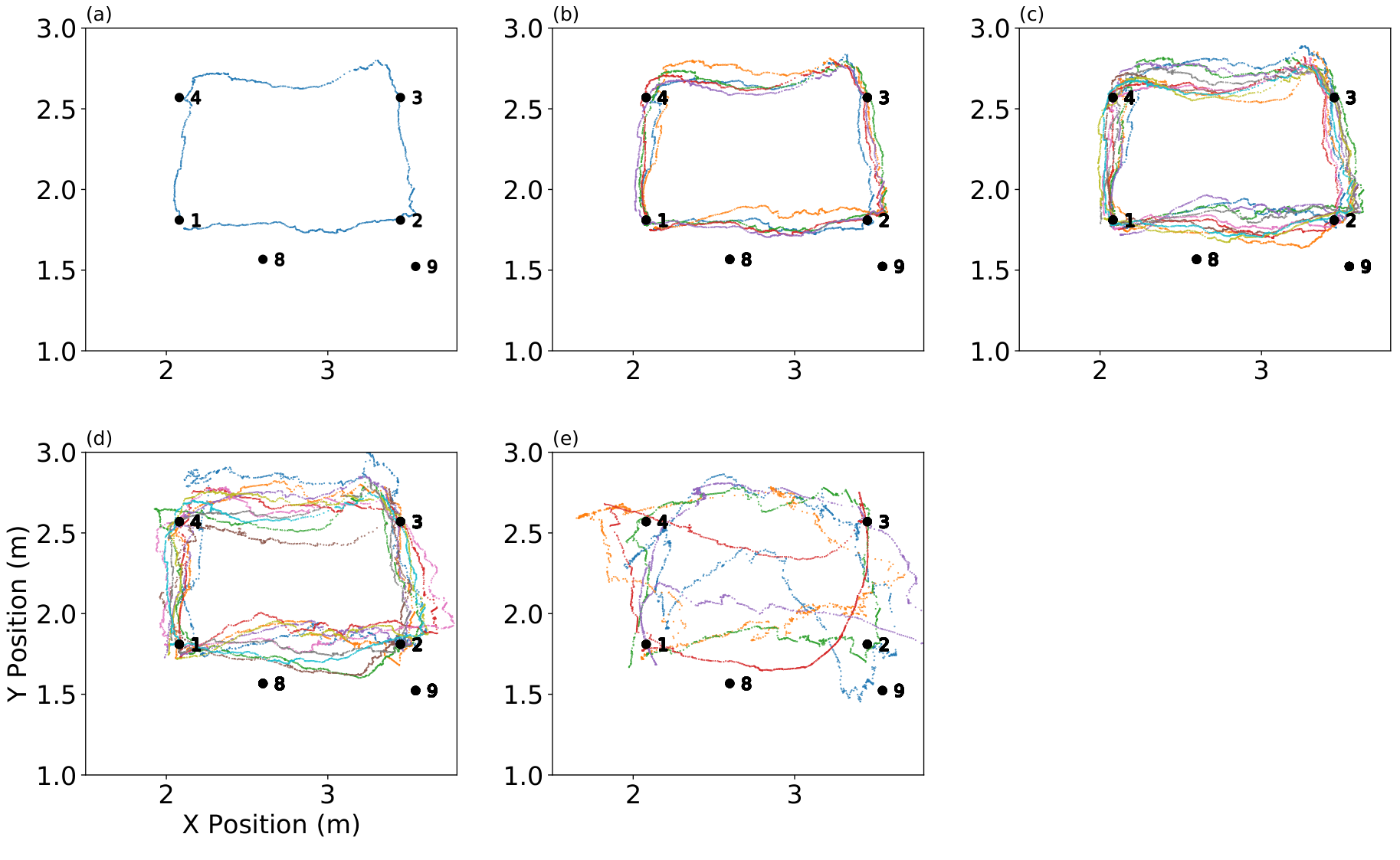
For the PCA mapping, it is problematic to drop an array as either the PCA has to be recalculated without the array or the missing DOA from that array should be estimated. However, a simple solution is to omit that part of the DOA vector, but still use the same SVD vector based on all arrays. Fig. 10 shows how this affects the estimation for the whole rectangle. Depending on which array is dropped it projects to quite different area of the PCA. Thus, if an array is dropped, it does not give clear results for one observation. However, Fig. 10 shows that if we drop an entire array in computing the SVD with the calibration points and for the PCA, the metasurface shows a consistent result with the rectangle of sources clearly mapped.
The non-linear mapping (4) maps to the domain and therefore shows good results as long as there are sufficient arrays to perform the mapping, see Fig. 11. Since all calibration points and measurements are in a horizontal plane, even just one array (Fig. 11e) can do well in the mapping provided its DOA are nearly perpendicular to the plane of motion of the sound source. Here, the ceiling arrays (array-2, array-3, array-4) have their DOAs approximately perpendicular to the plane of the motion of the sound source. For one array, the arrays on the walls (array-0, array-1) have DOAs to close to parallel with the source plane, and hence do not give good result. There is significant stability improvement in increasing to two arrays (Fig. 11d).
Figure 12 illustrate the difference in (a) affine mapping (4) and (b) PCA mapping for each observation 50% chance one array is dropped, which array is dropped is decided uniformly. In this figure the -matrix is determined by the calibration points on the table (points 1–4). Similar to the above results, the figure shows that simple PCA is noisy with large uncertainty.
V Conclusion
Sound source localization in rooms with redundant un-localized arrays are discussed. Each array performs the direction of arrival (DOA) estimation independently and feed it to a cluster where the DOA from all arrays are concatenated. The DOAs can then be used for source localization, either in principal component space or directly mapping to the room.
The method was demonstrated with five circular microphone arrays at un-measured locations in an office. Both methods work well for tracking a source in a room. The direct mapping to room coordinates is more robust to array failures. The methods demonstrated here provides a step towards monitoring activities in smart home with little installation effort.
Acknowledgements
We appreciate initial assistance of Brian Wang and Yifan Wu.
References
- [1] F. Grondin and F. Michaud. Lightweight and optimized sound source localization and tracking methods for open and closed microphone array configurations. Robot. Autonom. Syst., 113:63–80, 2019.
- [2] F. Grondin, D. Létourneau, F. Ferland, V. Rousseau, and F. Michaud. The ManyEars open framework. Autonom. Robots, 34(3):217–232, 2013.
- [3] C. Debes, A. Merentitis, S. Sukhanov, M. Niessen, N. Frangiadakis, and A. Bauer. Monitoring activities of daily living in smart homes: Understanding human behavior. IEEE Signal Process. Mag., 33(2):81–94, 2016.
- [4] A Fleury, M. Vacher, and N. Noury. SVM-based multimodal classification of activities of daily living in health smart homes: sensors, algorithms, and first experimental results. IEEE Trans. Inform. Techn. biomedicine, 14(2):274–283, 2009.
- [5] T Virtanen, M.D Plumbley, and D. Ellis. Computational analysis of sound scenes and events. Springer, 2018.
- [6] R. Serizel, N. Turpault, A. Shah, and J. Salamon. Sound event detection in synthetic domestic environments. In Proc. of IEEE ICASSP, pages 86–90, 2020.
- [7] T.K. Chan and C. S. Chin. A comprehensive review of polyphonic sound event detection. IEEE Access, 8:103339–103373, 2020.
- [8] C. Zhang, D. Florencio, D. E. Ba, and Z. Zhang. Maximum likelihood sound source localization and beamforming for directional microphone arrays in distributed meetings. IEEE Trans. Multimed., 10(3):538–548, 2008.
- [9] P. Aarabi. The fusion of distributed microphone arrays for sound localization. EURASIP J. Adv. Signal Proces., 2003(4):860465, 2003.
- [10] N.D. Gaubitch, W.B. Kleijn, and R. Heusdens. Auto-localization in ad-hoc microphone arrays. In Proc. of IEEE ICASSP, pages 106–110, 2013.
- [11] M. Cobos, F. Antonacci, A. Alexandridis, A. Mouchtaris, and B. Lee. A survey of sound source localization methods in wireless acoustic sensor networks. Wirel. Commun. Mob. Com., 2017, 2017.
- [12] M.S. Brandstein and H.F. Silverman. A robust method for speech signal time-delay estimation in reverberant rooms. In Proc. of the IEEE ICASSP, volume 1, pages 375–378, 1997.
- [13] H.L. Van Trees. Optimum Array Processing, chapter 1–10. Wiley-Interscience, New York, 2002.
- [14] A. Xenaki, P. Gerstoft, and K. Mosegaard. Compressive beamforming. J. Acoust. Soc. Am., 136(1):260–271, 2014.
- [15] D.P. Wipf and B.D. Rao. An empirical Bayesian strategy for solving the simultaneous sparse approximation problem. IEEE Trans. Signal Process., 55(7):3704–3716, 2007.
- [16] P. Gerstoft, A. Xenaki, and C. F. Mecklenbräuker. Multiple and single snapshot compressive beamforming. J. Acoust. Soc. Am., 138(4):2003–2014, 2015.
- [17] P. Gerstoft, C.F. Mecklenbräuker, W. Seong, and M.J. Bianco. Introduction to compressive sensing in acoustics. J. Acoust. Soc. Am., 143(6):3731–3736, 2018.
- [18] P. Gerstoft, C. F. Mecklenbräuker, A. Xenaki, and S. Nannuru. Multisnapshot sparse Bayesian learning for DOA. IEEE Signal Process. Lett., 23(10):1469–1473, 2016.
- [19] S. Nannuru, K.L. Gemba, P. Gerstoft, W.S. Hodgkiss, and C.F. Mecklenbräuker. Sparse Bayesian learning with multiple dictionaries. Signal Process., 159:159–170, 2019.
- [20] P. Gerstoft, S. Nannuru, C.F. Mecklenbräuker, and G. Leus. DOA estimation in heteroscedastic noise. Signal Process., 161:63–73, 2019.
- [21] K.L. Gemba, S. Nannuru, and P. Gerstoft. Robust ocean acoustic localization with sparse Bayesian learning. IEEE J Sel. Topics Signal Process., 13:49–60, 2019.
- [22] R. Schmidt. Multiple emitter location and signal parameter estimation. IEEE Trans Ant. Prop., 34(3):276–280, 1986.
- [23] K. Nakamura, K. Nakadai, F. Asano, and G. Ince. Intelligent sound source localization and its application to multimodal human tracking. In Proc. of IEEE/RSJ IROS, pages 143–148, 2011.
- [24] K. Nakamura, K. Nakadai, , and G. Ince. Real-time super-resolution sound source localization for robots. In Proc. of IEEE/RSJ IROS, pages 694–699, 2012.
- [25] E. Ozanich, P. Gerstoft, and H. Niu. A feedforward neural network for direction-of-arrival estimation. J. Acoust. Soc. Am., 147(3):2035–2048, 2020.
- [26] A. Barthelme and W. Utschick. A machine learning approach to DoA estimation and model order selection for antenna arrays with subarray sampling. arXiv preprint arXiv:2009.12858, 2020.
- [27] Florian Meyer, Bernhard Etzlinger, Zhenyu Liu, Franz Hlawatsch, and Moe Z Win. A scalable algorithm for network localization and synchronization. IEEE Internet of Things Journal, 5(6):4714–4727, 2018.
- [28] D. Di Carlo, A. Deleforge, and N. Bertin. Mirage: 2D source localization using microphone pair augmentation with echoes. In Proc. of IEEE ICASSP, pages 775–779, 2019.
- [29] C. Rascon, G. Fuentes, and I. Meza. Lightweight multi-doa tracking of mobile speech sources. EURASIP, 2015(1):1–16, 2015.
- [30] M.J. Bianco, P. Gerstoft, J. Traer, E. Ozanich, M.A. Roch, S. Gannot, and C.-A. Deledalle. Machine learning in acoustics: Theory and applications. J. Acoust. Soc. Am., 146(5):3590–3628, 2019.
- [31] S. Chakrabarty and E. A. P. Habets. Multi-speaker doa estimation using deep convolutional networks trained with noise signals. IEEE J. Sel. Topics Signal Process., 13(1):8–21, March 2019.
- [32] S. Adavanne, A. Politis, J. Nikunen, and T. Virtanen. Sound event localization and detection of overlapping sources using convolutional recurrent neural networks. IEEE J. Sel. Topics Signal Process., 2019.
- [33] Y. Wu, R Ayyalasomayajula, M. J. Bianco, D. Bharadia, and P. Gerstoft. Blind sound source localization based on deep learning. in press ICASSP, arXiv preprint arXiv:2010.14420, 2020.
- [34] M.J. Bianco, S. Gannot, and P. Gerstoft. Semi-supervised source localization with deep generative modeling. IEEE MLSP, 2020.
- [35] M. J. Bianco, S. Gannot, E. Fernandez-Grande, and P. Gerstoft. Semi-supervised source localization in reverberant environments with deep generative modeling. arXiv preprint arXiv:2101.10636, 2021.
- [36] Y. Hu, P. N. Samarasinghe, S. Gannot, and T. D. Abhayapala. Semi-supervised multiple source localization using relative harmonic coefficients under noisy and reverberant environments. IEEE/ACM Trans. Audio, Speech, Lang. Process, 28:3108–3123, 2020.
- [37] M. Liu, L Cheng, K. Qian, J. Wang, J. Wang, and Y. Liu. Indoor acoustic localization: a survey. Human-centric Comp. Inf. Sci., 10(1):2, 2020.
- [38] K. Nakadai, T. Lourens, H. G. Okuno, and H. Kitano. Active audition for humanoid. In Proc. Natl. Conf. Artif. Intell., pages 832–839, 2000.
- [39] K.L. Gemba, S. Nannuru, and P. Gerstoft. Robust ocean acoustic localization with sparse bayesian learning. IEEE J. Sel. Topics Signal Process., 13(1):49–60, 2019.
- [40] S. Zhao, S. Ahmed, Y. Liang, K. Rupnow, D. Chen, and D.L. Jones. A real-time 3D sound localization system with miniature microphone array for virtual reality. In Proc. of IEEE ICIEA, pages 1853–1857, 2012.
- [41] J.-S. Lauzon, F. Grondin, D. Létourneau, A. Lussier Desbiens, and F. Michaud. Localization of RW-UAVs using particle filtering over distributed microphone arrays. In Proc. of IEEE/RSJ IROS, pages 2479–2484, 2017.
- [42] X. Xiao, S. Zhao, D.H.H. Nguyen, X. Zhong, D.L. Jones, E.S. Chng, and H. Li. The NTU-ADSC systems for reverberation challenge 2014. In Proc. of REVERB Challenge Workshop, 2014.
- [43] X. Dang and H. Zhu. A feature-based data association method for multiple acoustic source localization in a distributed microphone array. J. Acoust. Soc. Am., 149(1):612–628, 2021.
- [44] D.L. Mills. On the accuracy and stability of clocks synchronized by the network time protocol in the internet system. ACM SIGCOMM Computer Comm. Review, 20(1):65–75, 1989.