Departure-based asymptotic stochastic order for random processes

Stochastic orders are extensively studied in the literature in the context of comparing random variables. They have been extended to compare random vectors, but not much exploration has been done in the context of comparing stochastic processes. In the present work, we attempt to compare stochastic processes in an asymptotic sense. Let $X$ and $Y$ be two random variables. $X$ is said to be smaller than $Y$ in usual stochastic order (denoted by $X\leqslant_{\textnormal{st}}Y$) if, for every $x\in\mathbb{R}$, we have $P(X>x)\leqslant P(Y>x)$. We say that $X$ is equal to $Y$ in usual stochastic order (denoted by $X=_{st}Y$) if $X\leqslant_{\textnormal{st}}Y$ and $Y\leqslant_{\textnormal{st}}X$. If $F_{X}$ and $F_{Y}$ denote the respective cdfs of $X$ and $Y$, then the condition $P(X>x)\leqslant P(Y>x)$ can be written as $F_{X}(x)\geqslant F_{Y}(x)$ for every $x\in\mathbb{R}$. Let $\left\{x_{1},x_{2},\ldots,x_{n}\right\}$ and $\left\{y_{1},y_{2},\ldots,y_{n}\right\}$ be two samples taken from two populations. The empirical cdfs based on these two samples are defined respectively by $F_{n}(x)=n^{-1}\sum_{i=1}^{n}1_{(x_{i},\infty)}(x)$ and $G_{n}(x)=n^{-1}\sum_{i=1}^{n}1_{(y_{i},\infty)}(x)$, for every $x\in\mathbb{R}$, where for any $A\subseteq\mathbb{R}$, the indicator function $1_{A}:\mathbb{R}\to\{0,1\}$ is given by $1_{A}(x)=1$ if $x\in A$ and equal to $0$ otherwise. Note that if $\hat{X}$ and $\hat{Y}$ respectively have the empirical cdfs $F_{n}$ and $G_{n}$, then $\hat{X}\leqslant\hat{Y}$ if and only if $x_{i:n}\leqslant y_{i:n}$ for every $i\in\left\{1,2,\ldots,n\right\}$, where $x_{i:n}$ and $y_{i:n}$ respectively denote the $i$th largest element from the samples $\left\{x_{1},x_{2},\ldots,x_{n}\right\}$ and $\left\{y_{1},y_{2},\ldots,y_{n}\right\}$. In other words, $\hat{X}\leqslant_{\textnormal{st}}\hat{Y}$ if and only if $\#\left\{i\in\left\{1,2,\ldots,n\right\}:x_{i:n}\leqslant y_{i:n}\right\}/n=1$. The ratio $\#\left\{i\in\left\{1,2,\ldots,n\right\}:x_{i:n}\leqslant y_{i:n}\right\}/n$ is Galton’s rank order statistic (see Gross & Holland 1968, Hodges 1955), which goes all the way back to a correspondence between Galton and Darwin in 1876, in the context of analyzing data from the latter’s experiments on cross and self fertilization of plants (see Darwin 1878). It is well-known that usual stochastic order is a partial order.

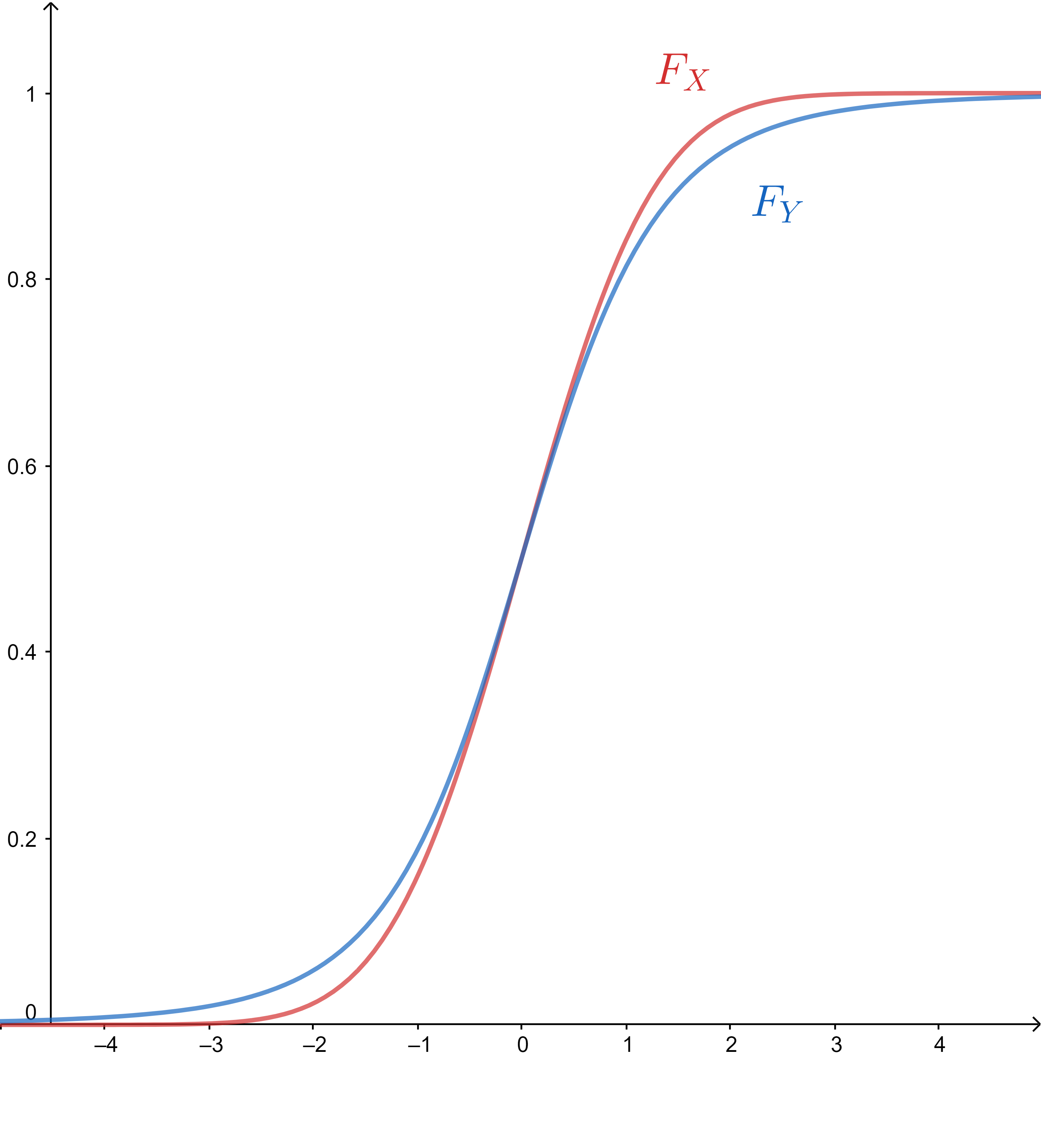
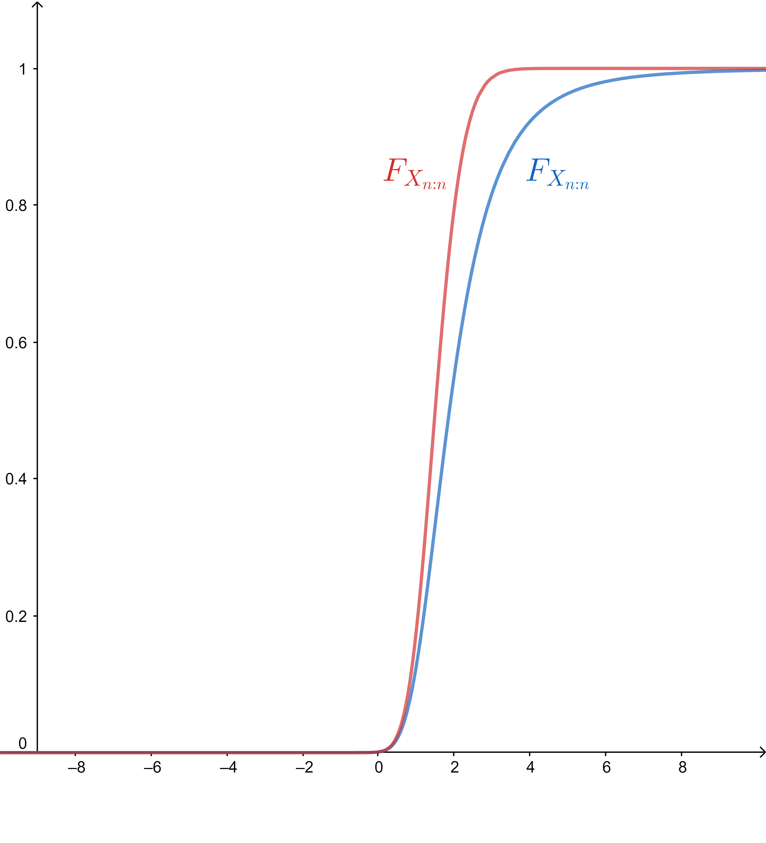
It is often observed that two cdfs $F_{X}$ and $F_{Y}$ cross each other, indicating that usual stochastic order cannot exist between $X$ and $Y$. However, $F_{X}(x)$ and $F_{Y}(x)$ may be extremely close in the region where $F_{X}$ dominates $F_{Y}$, but differ significantly where $F_{Y}$ dominates $F_{X}$ (see Fig. 1(b) for a situation where such a phenomenon occurs). To address this situation, one possible approach is to consider certain measures based on the region where the defining condition, or a characterizing condition is violated, and the extent of that violation. Following this approach we had defined a number of asymptotic stochastic orders in Ghosh & Nanda 2021. An alternative approach, which is the focus of the present paper, is to consider measures of departure from the usual stochastic order. Leshno & Levy 2002 introduced the notion of almost stochastic dominance in the context of risk aversion and considered the following measure, which can be considered as a measure of departure from the usual stochastic order $X\leqslant_{\textnormal{st}}Y$.

where $B_{0}=\{x\in\mathbb{R}:F_{X}(x)<F_{Y}(x)\}$ and $\|\cdot\|_{1}$ denotes the $L_{1}$ norm with respect to the Lebegue measure on $\mathbb{R}$. Despite its simplicity, asymptotic properties of this measure are not available in the literature. Recently, del Barrio et al. 2018 proposed and derived the asymptotic properties of a measure of departure from the usual stochastic order $X\leqslant_{\textnormal{st}}Y$, based on the $L_{2}$-Wasserstein distance between two cdfs. The measure is motivated by the following characterization of usual stochastic order in terms of quantile functions.

Here $F_{X}^{-1}$ and $F_{Y}^{-1}$ denote the respective left continuous inverses of $F_{X}$ and $F_{Y}$, i.e. $F_{X}^{-1}(u)=\inf{\left\{x\in\mathbb{R}:F_{X}(x)\geqslant u\right\}}$ and $F_{Y}^{-1}(u)=\inf{\left\{x\in\mathbb{R}:F_{Y}(x)\geqslant u\right\}}$. For more details on characterizations and closure properties of the usual stochastic order, we refer to Shaked & Shanthikumar 2007. It is noted in Lehmann 1955 that the characterization of usual stochastic order in terms of the quantile functions, as stated in Proposition 1.1, is more intuitive than its definition. The measure of departure from $X\leqslant_{\textnormal{st}}Y$ proposed in del Barrio et al. 2018 is given by

where $A_{0}=\{u\in(0,1):F_{X}^{-1}(u)>F_{Y}^{-1}(u)\}$ and $\mathcal{W}_{2}(F_{X},F_{Y})$ is the $L_{2}$-Wesserstein distance between $F_{X}$ and $F_{Y}$, which has the following representation in terms of the corresponding quantile functions $F_{X}^{-1}$ and $F_{Y}^{-1}$.

It is well-known that if $F_{X}$ and $F_{Y}$ both have finite second order moment, then $\mathcal{W}_{2}(F_{X},F_{Y})$ is finite. Note that the measure of departure from $X\leqslant_{\textnormal{st}}Y$ varies between $0$ and $1$, achieving the extremes in the cases $X\leqslant_{\textnormal{st}}Y$ and $Y\leqslant_{\textnormal{st}}X$, respectively. When the usual stochastic order does not hold, the measure gives a quantification of stochastic dominance of $X$ over $Y$. In this paper, we introduce the notion of asymptotic stochastic order for stochastic processes, based on this measure of departure.

To motivate the idea, let us consider the following situation. Let $F_{X}$ and $F_{Y}$ be two cdfs with finite second order moments. Suppose that the right tail of $F_{X}$ is heavier than that of $F_{Y}$ in the sense that there exists $c\in\mathbb{R}$ such that $F_{X}(x)>F_{Y}(x)$, whenever $x>c$. Now, if one takes two samples (of same size) of random observations, the first one from $F_{X}$ and the second from $F_{Y}$, then one may expect that the largest observation from the first sample is smaller than that from the second sample. To be more precise, let $X_{1},X_{2},\ldots,X_{n}$ be a random sample from the standard normal distribution and $Y_{1},Y_{2},\ldots,Y_{n}$ be the same from $t$ distribution with $4$ degrees of freedom. Clearly, none of the two distributions dominate the other in usual stochastic order (see Fig. 1(a)). However, our intuition suggests that the largest order statistics $X_{n:n}$ and $Y_{n:n}$, from the respective samples should reflect the relative tail behaviour of the parent distributions. In particular, $Y_{n:n}$ should dominate $X_{n:n}$ in some stochastic sense. The respective cdfs of $X_{n:n}$ and $Y_{n:n}$ are given by $F_{X_{n:n}}(x)=(F_{X}(x))^{n}$ and $F_{Y_{n:n}}(x)=(F_{Y}(x))^{n}$ for every $x\in\mathbb{R}$. It follows that $X_{n:n}\leqslant_{\textnormal{st}}Y_{n:n}$ if and only if $X_{1}\leqslant_{\textnormal{st}}Y_{1}$. Hence, the usual stochastic order between $X_{n:n}$ and $Y_{n:n}$ does not hold in the case explained. However, observation of the cdfs of $X_{n:n}$ and $Y_{n:n}$ suggests that stochastic order may exist in an approximate sense even when the sample size $n$ is as small as $10$ (see Fig. 1(b)).

This motivate us to examine stochastic order that may exist between $X_{n:n}$ and $Y_{n:n}$ in some asymptotic sense. In this work, we find out that this is indeed the case, as indicated by the following proposition, which follows from a more general result, Theorem 3.9, in Section 3 (see Remark 3.13).

Note that, since $F_{Y}(c)<1$, we can choose $\epsilon>0$ such that $F_{Y}(c)/(1-\epsilon)<1$ and hence the right hand side of (1.3) goes to $0$, as $n\to\infty$. Consequently, the measure of departure from $X_{n:n}\leqslant_{\textnormal{st}}Y_{n:n}$ shrinks to $0$, as $n\to\infty$. In the example with standard normal distribution and $t_{4}$ distribution, stated above, we have $c=0$ and consequently $F_{Y}(c)=1/2$. It is interesting to observe that the relative behavior of $F_{X}$ and $F_{Y}$ in the region $(-\infty,c)$ has no effect on the result. Building upon this particular observation, we consider the problem of comparing not only other order statistics, but also certain stochastic processes with common unbounded above index set $T\subseteq\mathbb{R}$ as well.

Any function which is nondecreasing with $\phi(0)=0$ and $\phi(1)=1$ is called a distortion function or probability transformation function (see Denneberg 1994). The general idea is that given a class of distortion functions $\left\{\phi_{t}:t\in T\right\}$, satisfying some asymptotic properties, if the baseline cdfs $F_{X}$ and $F_{Y}$ agree on the desired stochastic order around a finite set of points (dictated by the asymptotic behaviour of the map $t\mapsto\phi_{t}$), then the stochastic processes $\left\{\phi_{t}(F_{X}):t\in T\right\}$ and $\left\{\phi_{t}(F_{Y}):t\in T\right\}$ admit asymptotic stochastic order (see Section 2). The way the baseline cdfs behave away from the specified finite number of points has no effect on the asymptotic stochastic order (see Section 4).

Throughout the paper, we stick to the following notations and conventions. For any interval $I$, we denote its length by $\lvert I\rvert$ and, for any $A\subseteq\mathbb{R}$, we denote its Lebesgue measure by $l(A)$. For a function $f:B\to\mathbb{R}$, we define the $f$-image of a set $A\subseteq B$ as $f(A)=\{f(x):x\in A\}$. Throughout the paper, the inverse of a cdf $F$ is defined as the left continuous inverse of $F$, which becomes the unique inverse if $F$ is strictly increasing. For any function $f:[0,1]\to\mathbb{R}$ which is continuously differentiable in $(0,1)$, we define the derivative of $f$ at the endpoints, i.e. $0$ and $1$, respectively by $f^{\prime}(0)=\lim_{u\to 0+}f^{\prime}(u)$ and $f^{\prime}(1)=\lim_{u\to 1-}f^{\prime}(u)$. For an arbitrary set $T\subseteq\mathbb{R}$ which is unbounded above, the limit of a real-valued function $t\mapsto\psi(t)$ defined on $T$, as $t\to\infty$, is considered in the usual sense, i.e. $\lim_{t\to\infty}\psi(t)\equiv\lim_{t\to\infty;\,t\,\in\,T}\psi(t)=a\in\mathbb{R}\cup\{-\infty,\infty\}$ if, for every sequence $\left\{t_{n}\in T:n\in\mathbb{N}\right\}$ with $t_{n}\to\infty$, as $n\to\infty$, we have $\lim_{n\to\infty}\psi(t_{n})=a$. We follow the notations listed below throughout. Let $Z$ be a random variable. We denote the cdf of $Z$ by $F_{Z}$ and the quantile function of $Z$ by $F_{Z}^{-1}$, which is the left-continuous inverse of $F_{Z}$. Let $X$ and $Y$ be two random variables. Then we denote

The rest of the paper is structured as follows. In Section 2, we define the departure-based asymptotic stochastic order and discuss its properties. In Section 3, we derive sufficient conditions for departure-based asymptotic stochastic order between $1+\left[(n-1)\gamma_{n}\right]$th order statistics from two different homogeneous samples, where one may choose the sequence $\{\gamma_{n}\}$ which converges to $\gamma\in[0,1]$ appropriately to take any extreme or central order statistic into account. In Section 4, we have extended the idea to stochastically compare certain stochastic processes in an asymptotic sense. In Section 5, we apply the concept to make asymptotic stochastic comparison of mixtures of order statistics as well as record values from two different homogeneous samples.

Let $\left\{X_{t}:t\in T\right\}$ and $\left\{Y_{t}:t\in T\right\}$ be two stochastic processes, where $T$ ($\subseteq\mathbb{R}$) is unbounded above and the state space is $\mathbb{R}$. Note that when $T=\mathbb{N}$ (resp. $T=[0,\infty)$), the processes become discrete-time (resp. continuous-time) stochastic processes. Now it may happen that there does not exist any $t\in T$ such that $X_{t}\leqslant_{\textnormal{st}}Y_{t}$ but, as $t\to\infty$, it increasingly gets closer to $X_{t}\leqslant_{\textnormal{st}}Y_{t}$, in some sense. The measure in (1.1) gives us a way to mathematically address such a situation. Observe that if $\mathcal{W}_{2}(F_{X},F_{Y})=0$, then $\varepsilon_{\mathcal{W}_{2}}(F_{X},F_{Y})$ has $0/0$ form, and hence is undefined. To reflect the fact that $X\leqslant_{\textnormal{st}}X$ for any random variable $X$, we use the convention that $\varepsilon_{\mathcal{W}_{2}}(F_{X},F_{Y})=0$ if $\mathcal{W}_{2}(F_{X},F_{Y})=0$. Again, observe that if $\int_{A_{0}}(F_{X}^{-1}(u)-F_{Y}^{-1}(u))^{2}\,du=\infty$, then $\varepsilon_{\mathcal{W}_{2}}(F_{X},F_{Y})$ has $\infty/\infty$ form, and hence is undefined. In this case, we use the convention that $\varepsilon_{\mathcal{W}_{2}}(F_{X},F_{Y})=1$.

Now we discuss some properties of the departure-based asymptotic stochastic order.

Let $\left\{X_{t}:t\in T\right\}$ be a stochastic process. Then $X_{t}\leqslant_{\textnormal{d-ast}}X_{t}$, as $t\to\infty$, i.e. departure-based asymptotic stochastic order is reflexive. To see this, note that, for every $t\in T$, we have $\mathcal{W}_{2}(F_{X_{t}},F_{X_{t}})=0$ and hence $\lim_{t\to\infty}\varepsilon_{\mathcal{W}_{2}}(F_{X_{t}},F_{X_{t}})=0$, giving $X_{t}\leqslant_{\textnormal{d-ast}}X_{t}$, as $t\to\infty$. Again, departure-based asymptotic stochastic order is antisymmetric by definition, i.e., for any two stochastic processes $\left\{X_{t}:t\in T\right\}$ and $\left\{Y_{t}:t\in T\right\}$, $X_{t}\leqslant_{\textnormal{d-ast}}Y_{t}$, as $t\to\infty$ and $Y_{t}\leqslant_{\textnormal{d-ast}}X_{t}$, as $t\to\infty$ imply $X_{t}=_{\textnormal{ast}}Y_{t}$, as $t\to\infty$. The transitivity property, however, is not so straightforward and requires additional conditions, as shown in the next result.

References

• Ahsanullah & Nevzorov [2011] Ahsanullah, M. & Nevzorov, V. B. (2011). Record Statistics. In: International Encyclopedia of Statistical Science, Lovric, M. (Ed.). 1195–1202. Springer Berlin Heidelberg.
• Chandler [1952] Chandler, K. N. (1952). The distribution and frequency of record values. Journal of the Royal Statistical Society. Series B, 14(2), 220–228.
• Darwin [1878] Darwin, C. (1878). The Effect of Cross- and Self-fertilization in the Vegetable Kingdom (2nd ed.). John Murray, London.
• del Barrio et al. [2018] del Barrio, E., Cuesta-Albertos, J. A., & Matrán, C. (2018). An Optimal Transportation Approach for Assessing Almost Stochastic Order. In: The Mathematics of the Uncertain: A Tribute to Pedro Gil, Gil, E., Gil, E., Gil, J. and Gil, M. (Eds.), 33–44. Springer International Publishing.
• Denneberg [1994] Denneberg, D. (1994). Non-Additive Measure and Integral. Springer, Netherlands.
• Dziubdziela & Kopociński [1976] Dziubdziela, W. & Kopociński, B. (1976). Limiting properties of the k-th record values. Applicationes Mathematicae, 15(2), 187–190.
• Ghosh & Nanda [2021] Ghosh, S. & Nanda, A. K. (2021). Asymptotic Stochastic Comparison of Random Processes. arXiv:2103.01720.
• Gross & Holland [1968] Gross, S. & Holland, P. (1968). The distribution of galton’s statistic. The Annals of Mathematical Statistics, 39(6), 2114–2117.
• Hodges [1955] Hodges, J. L., J. (1955). Galton’s rank order test. Biometrika, 42, 261–262.
• Lehmann [1955] Lehmann, E. L. (1955). Ordered families of distributions. Annals of Mathematical Statistics, 26(3), 399–419.
• Leshno & Levy [2002] Leshno, M. & Levy, H. (2002). Preferred by “all” and preferred by “most” decision makers: Almost stochastic dominance. Management Science, 48(8), 1074–1085.
• Samaniego [2007] Samaniego, F. J. (2007). System Signatures and their Applications in Engineering Reliability. Springer, New York.
• Shaked & Shanthikumar [2007] Shaked, M. & Shanthikumar, J. G. (2007). Stochastic Orders. Springer, New York.
6. Appendix
Proof of Lemma 3.1.
Note that, for any cdf FF, we have F⁡(F−1​(u))⩾uF(F^{-1}(u))\geqslant u, for every u∈(0,1)u\in(0,1), where equality holds if FF is continuous and F−1​(F​(x))⩽xF^{-1}(F(x))\leqslant x, for every x∈ℝx\in\mathbb{R}, where equality holds if FF is strictly increasing. Let x∈B0x\in B_{0}. Then FX​(x)<FY​(x)F_{X}(x)<F_{Y}(x). Suppose, for the sake of contradiction, that FX​(x)∉A0F_{X}(x)\notin A_{0}. Then FY−1​(FY​(x))=x=FX−1​(FX​(x))⩽FY−1​(FX​(x))F_{Y}^{-1}(F_{Y}(x))=x=F_{X}^{-1}(F_{X}(x))\leqslant F_{Y}^{-1}(F_{X}(x)). By nondecreasingness of FYF_{Y}, we have FX​(x)⩾FY​(x)F_{X}(x)\geqslant F_{Y}(x), a contradiction. Hence FX​(x)∈A0F_{X}(x)\in A_{0}. Since x∈B0x\in B_{0} is arbitrary, we have FX​(B0)⊆A0F_{X}(B_{0})\subseteq A_{0}. Again, starting with x∈B0x\in B_{0} and FY​(x)∉A0F_{Y}(x)\notin A_{0}, we similarly have A0⊆FX​(B0)A_{0}\subseteq F_{X}(B_{0}). Hence A0=FX​(B0)A_{0}=F_{X}(B_{0}). Similarly, A0=FY​(B0)A_{0}=F_{Y}(B_{0}). Interchanging the role of FXF_{X} and FYF_{Y}, we have A1=FX​(B1)=FY​(B1)A_{1}=F_{X}(B_{1})=F_{Y}(B_{1}). Again, A2=A0∪A1=FX​(B0)∪FX​(B1)=FX​(B0∪B1)=FX​(B2)A_{2}=A_{0}\cup A_{1}=F_{X}(B_{0})\cup F_{X}(B_{1})=F_{X}(B_{0}\cup B_{1})=F_{X}(B_{2}). In a similar manner, we obtain A2=FY​(B2)A_{2}=F_{Y}(B_{2}). ∎
Proof of Proposition 3.5.
Let us denote the fractional part of (n−1)​γn(n-1)\gamma_{n} by {(n−1)​γn}\left\{(n-1)\gamma_{n}\right\}. Then, we have
ϕn,γn′​(t)ϕn,γn′​(s)=(s⁡(1−t)t⁡(1−s)){(n−1)​γn}​((ts)γn​(1−t1−s)1−γn)n−1.\frac{\phi_{n,\gamma_{n}}^{\prime}(t)}{\phi_{n,\gamma_{n}}^{\prime}(s)}=\left(\frac{s(1-t)}{t(1-s)}\right)^{\left\{(n-1)\gamma_{n}\right\}}\left(\left(\frac{t}{s}\right)^{\gamma_{n}}\left(\frac{1-t}{1-s}\right)^{1-\gamma_{n}}\right)^{n-1}.
Considering the cases t>st>s, t<st<s and t=st=s separately, it is easy to see that
(s⁡(1−t)t⁡(1−s)){(n−1)​γn}⩽(s⁡(1−t)t⁡(1−s))12−12⋅sign​(t−s),\left(\frac{s(1-t)}{t(1-s)}\right)^{\left\{(n-1)\gamma_{n}\right\}}\leqslant\left(\frac{s(1-t)}{t(1-s)}\right)^{\frac{1}{2}-\frac{1}{2}\,\cdot\,\text{sign}{(t-s)}},
with equality if and only if t=st=s. Again,
((ts)γn​(1−t1−s)1−γn)n−1=((ts)γ​(1−t1−s)1−γ)n−1​(t⁡(1−s)s⁡(1−t))(n−1)​(γn−γ).\left(\left(\frac{t}{s}\right)^{\gamma_{n}}\left(\frac{1-t}{1-s}\right)^{1-\gamma_{n}}\right)^{n-1}=\left(\left(\frac{t}{s}\right)^{\gamma}\left(\frac{1-t}{1-s}\right)^{1-\gamma}\right)^{n-1}\left(\frac{t(1-s)}{s(1-t)}\right)^{(n-1)(\gamma_{n}-\gamma)}.
Since, |γn−γ|=O⁡(1/n)\lvert\gamma_{n}-\gamma\rvert=O(1/n), there exists K>0K>0 and N∈ℕN\in\mathbb{N} such that, for every n⩾Nn\geqslant N, |γn−γ|⩽K/n\lvert\gamma_{n}-\gamma\rvert\leqslant K/n, which in turn implies that |γn−γ|⩽K/(n−1)\lvert\gamma_{n}-\gamma\rvert\leqslant K/(n-1), i.e. −K⩽(n−1)​(γn−γ)⩽K-K\leqslant(n-1)(\gamma_{n}-\gamma)\leqslant K. Considering the cases t<st<s, t>st>s and t=st=s separately, we can see that
(t⁡(1−s)s⁡(1−t))(n−1)​(γn−γ)⩽(t⁡(1−s)s⁡(1−t))K⋅sign​(t−s).\left(\frac{t(1-s)}{s(1-t)}\right)^{(n-1)(\gamma_{n}-\gamma)}\leqslant\left(\frac{t(1-s)}{s(1-t)}\right)^{K\,\cdot\,\text{sign}{(t-s)}}.
Hence,
ϕn,γn′​(t)ϕn,γn′​(s)\displaystyle\frac{\phi_{n,\gamma_{n}}^{\prime}(t)}{\phi_{n,\gamma_{n}}^{\prime}(s)} ⩽(s⁡(1−t)t⁡(1−s))12−12⋅sign​(t−s)​(t⁡(1−s)s⁡(1−t))K⋅sign​(t−s)​((ts)γ​(1−t1−s)1−γ)n−1\displaystyle\leqslant\left(\frac{s(1-t)}{t(1-s)}\right)^{\frac{1}{2}-\frac{1}{2}\,\cdot\,\text{sign}{(t-s)}}\left(\frac{t(1-s)}{s(1-t)}\right)^{K\,\cdot\,\text{sign}{(t-s)}}\left(\left(\frac{t}{s}\right)^{\gamma}\left(\frac{1-t}{1-s}\right)^{1-\gamma}\right)^{n-1}
=(s⁡(1−t)t⁡(1−s))12−(K+12)⋅sign​(t−s)​((ts)γ​(1−t1−s)1−γ)n−1.\displaystyle=\left(\frac{s(1-t)}{t(1-s)}\right)^{\frac{1}{2}-(K+\frac{1}{2})\,\cdot\,\text{sign}{(t-s)}}\left(\left(\frac{t}{s}\right)^{\gamma}\left(\frac{1-t}{1-s}\right)^{1-\gamma}\right)^{n-1}.
Now, the proof follows by choosing C⁡(t,s)=(s⁡(1−t)t⁡(1−s))12−(K+12)⋅sign​(t−s)C(t,s)=\left(\frac{s(1-t)}{t(1-s)}\right)^{\frac{1}{2}-(K+\frac{1}{2})\,\cdot\,\text{sign}{(t-s)}}. ∎
Proof of Proposition 3.15.
To prove the first part, note that
limn→∞P{Bn,u⩾1+[(n−1)γn]}\displaystyle\lim_{n\to\infty}P\left\{B_{n,u}\geqslant 1+\left[(n-1)\gamma_{n}\right]\right\} =limn→∞P{Bn,u⩾12+[(n−1)γn]}\displaystyle=\lim_{n\to\infty}P\left\{B_{n,u}\geqslant\frac{1}{2}+\left[(n-1)\gamma_{n}\right]\right\}
(6.1) =limn→∞P{Z>12+[(n−1)​γn]−n​un​u​(1−u)},\displaystyle=\lim_{n\to\infty}P\left\{Z>\frac{\frac{1}{2}+\left[(n-1)\gamma_{n}\right]-nu}{\sqrt{nu(1-u)}}\right\},
where the last equality is due to CLT and ZZ has the standard normal distribution. Now, using the hypothesis |γn−γ|=O⁡(1/n)\lvert\gamma_{n}-\gamma\rvert=O(1/n), we have
12+[(n−1)​γn]−n​un​u​(1−u)=O⁡(n)​(γ−u)+O⁡(1/n),\displaystyle\frac{\frac{1}{2}+\left[(n-1)\gamma_{n}\right]-nu}{\sqrt{nu(1-u)}}=O(\sqrt{n})(\gamma-u)+O(1/\sqrt{n}),
Denoting the cdf of standard normal distribution by Φ\Phi, we have from (6) that
limn→∞P{Bn,u⩾1+[(n−1)γn]}=1−limn→∞Φ(O(n)(γ−u)+O(1/n)),\lim_{n\to\infty}P\left\{B_{n,u}\geqslant 1+\left[(n-1)\gamma_{n}\right]\right\}=1-\lim_{n\to\infty}\Phi(O(\sqrt{n})(\gamma-u)+O(1/\sqrt{n})),
which essentially implies (3.15) by continuity of Φ\Phi. To prove the second part, note that
limn→∞nP{Bn−1,u=[(n−1)γn]}=limn→∞nP{[(n−1)γn]−12<Bn−1,u<[(n−1)γn]+12}\displaystyle\lim_{n\to\infty}nP\left\{B_{n-1,u}=\left[(n-1)\gamma_{n}\right]\right\}=\lim_{n\to\infty}nP\left\{\left[(n-1)\gamma_{n}\right]-\frac{1}{2}<B_{n-1,u}<\left[(n-1)\gamma_{n}\right]+\frac{1}{2}\right\}
=limn→∞nP{[(n−1)​γn]−12−(n−1)​u(n−1)​u​(1−u)<Bn−1,u−(n−1)​u(n−1)​u​(1−u)<[(n−1)​γn]+12−(n−1)​u(n−1)​u​(1−u)}.\displaystyle=\lim_{n\to\infty}nP\left\{\frac{\left[(n-1)\gamma_{n}\right]-\frac{1}{2}-(n-1)u}{\sqrt{(n-1)u(1-u)}}<\frac{B_{n-1,u}-(n-1)u}{\sqrt{(n-1)u(1-u)}}<\frac{\left[(n-1)\gamma_{n}\right]+\frac{1}{2}-(n-1)u}{\sqrt{(n-1)u(1-u)}}\right\}.
Using CLT, the above expression becomes
limn→∞n⁡{Φ⁡([(n−1)​γn]+12−(n−1)​u(n−1)​u​(1−u))−Φ⁡([(n−1)​γn]−12−(n−1)​u(n−1)​u​(1−u))}\displaystyle\lim_{n\to\infty}n\left\{\Phi\left(\frac{\left[(n-1)\gamma_{n}\right]+\frac{1}{2}-(n-1)u}{\sqrt{(n-1)u(1-u)}}\right)-\Phi\left(\frac{\left[(n-1)\gamma_{n}\right]-\frac{1}{2}-(n-1)u}{\sqrt{(n-1)u(1-u)}}\right)\right\}
=limn→∞n⁡{Φ⁡((n−1)​(γn−u)+12−{(n−1)​γn}(n−1)​u​(1−u))−Φ⁡((n−1)​(γn−u)−12−{(n−1)​γn}(n−1)​u​(1−u))}\displaystyle=\lim_{n\to\infty}n\left\{\Phi\left(\frac{(n-1)(\gamma_{n}-u)+\frac{1}{2}-\left\{(n-1)\gamma_{n}\right\}}{\sqrt{(n-1)u(1-u)}}\right)-\Phi\left(\frac{(n-1)(\gamma_{n}-u)-\frac{1}{2}-\left\{(n-1)\gamma_{n}\right\}}{\sqrt{(n-1)u(1-u)}}\right)\right\}
=limn→∞n{Φ(n−1u⁡(1−u){γn−u+12​(n−1)−{(n−1)​γn}n−1})\displaystyle=\lim_{n\to\infty}n\Bigg\{\Phi\left(\sqrt{\frac{n-1}{u(1-u)}}\left\{\gamma_{n}-u+\frac{1}{2(n-1)}-\frac{\left\{(n-1)\gamma_{n}\right\}}{n-1}\right\}\right)
−Φ(n−1u⁡(1−u){γn−u−12​(n−1)−{(n−1)​γn}n−1})}\displaystyle\phantom{=\lim_{n\to\infty}n}-\Phi\left(\sqrt{\frac{n-1}{u(1-u)}}\left\{\gamma_{n}-u-\frac{1}{2(n-1)}-\frac{\left\{(n-1)\gamma_{n}\right\}}{n-1}\right\}\right)\Bigg\}
=limn→∞n​∫lnunϕ⁡(t)​𝑑t,\displaystyle=\lim_{n\to\infty}n\int_{l_{n}}^{u_{n}}\phi(t)dt,
where ln=n−1u⁡(1−u)​{γn−u−12​(n−1)−{(n−1)​γn}n−1}l_{n}=\sqrt{\frac{n-1}{u(1-u)}}\left\{\gamma_{n}-u-\frac{1}{2(n-1)}-\frac{\left\{(n-1)\gamma_{n}\right\}}{n-1}\right\} and un=n−1u⁡(1−u)​{γn−u+12​(n−1)−{(n−1)​γn}n−1}u_{n}=\sqrt{\frac{n-1}{u(1-u)}}\left\{\gamma_{n}-u+\frac{1}{2(n-1)}-\frac{\left\{(n-1)\gamma_{n}\right\}}{n-1}\right\} and ϕ\phi denotes the pdf of standard normal distribution. We consider the three cases u<γu<\gamma, u>γu>\gamma and u=γu=\gamma separately.
Case 1: u<γu<\gamma. Using the hypothesis |γn−γ|=O⁡(1/n)\lvert\gamma_{n}-\gamma\rvert=O(1/n), we have
(6.2) ln=(γ−u)​n−1u⁡(1−u)+O⁡(1/n).l_{n}=(\gamma-u)\sqrt{\frac{n-1}{u(1-u)}}+O(1/\sqrt{n}).
Thus, there exists N1∈ℕN_{1}\in\mathbb{N} such that 0<ln<un0<l_{n}<u_{n} whenever n⩾N1n\geqslant N_{1}. Then n​∫lnunϕ⁡(t)​𝑑t⩽n⁡(un−ln)​ϕ​(ln)n\int_{l_{n}}^{u_{n}}\phi(t)dt\leqslant n(u_{n}-l_{n})\phi(l_{n}), for every n⩾N1n\geqslant N_{1}. Now, n⁡(un−ln)=n/(n−1)​u​(1−u)n(u_{n}-l_{n})=n/\sqrt{(n-1)u(1-u)}. Also, from (6.2), we obtain ln⩾(γ−u)​n/2​u​(1−u)+O⁡(1/n)l_{n}\geqslant(\gamma-u)\sqrt{n}/\sqrt{2u(1-u)}+O(1/\sqrt{n}). Thus, there exists a natural number N2N_{2} large enough, such that ln⩾(γ−u)​n/4​u​(1−u)l_{n}\geqslant(\gamma-u)\sqrt{n}/\sqrt{4u(1-u)}, whenever n⩾N2n\geqslant N_{2}. Letting k1=(γ−u)/4​u​(1−u)k_{1}=(\gamma-u)/\sqrt{4u(1-u)}, we have ϕ(ln)=(2​π)−1exp(−ln2/2)⩽(2​π)−1exp(−k12n/2)\phi(l_{n})=(\sqrt{2\pi})^{-1}\exp{\left(-l_{n}^{2}/2\right)}\leqslant(\sqrt{2\pi})^{-1}\exp{\left(-k_{1}^{2}n/2\right)}, for every n⩾N2n\geqslant N_{2}. Thus, for every n⩾max⁡{N1,N2}n\geqslant\max{\{N_{1},N_{2}\}}, we have n(un−ln)ϕ(ln)⩽nexp(−k12n/2)/2​π​(n−1)​u​(1−u)n(u_{n}-l_{n})\phi(l_{n})\leqslant n\exp{\left(-k_{1}^{2}n/2\right)}/\sqrt{2\pi(n-1)u(1-u)}, which goes to 00, as n→∞n\to\infty.
Case 2: u>γu>\gamma. Let k2=2​(u−γ)/u⁡(1−u)k_{2}=2(u-\gamma)/u(1-u). On using the same chain of arguments as in Case 11, we obtain n(un−ln)ϕ(un)⩽nexp(−k22n/2)/2​π​(n−1)​u​(1−u)n(u_{n}-l_{n})\phi(u_{n})\leqslant n\exp{\left(-k_{2}^{2}n/2\right)}/\sqrt{2\pi(n-1)u(1-u)}, which goes to 00, as n→∞n\to\infty.
Case 3: u=γu=\gamma. Since ϕ\phi is continuous, by integral mean value theorem, there exists mn∈[ln,un]m_{n}\in\left[l_{n},u_{n}\right] such that
∫lnunϕ⁡(t)​𝑑t=(un−ln)​ϕ​(mn).\int_{l_{n}}^{u_{n}}\phi(t)dt=(u_{n}-l_{n})\phi(m_{n}).
Clearly, for every n∈ℕn\in\mathbb{N}, there exists αn∈[−1,1]\alpha_{n}\in\left[-1,1\right] such that
mn=n−1u⁡(1−u)​{γn−u+αn2​(n−1)−{(n−1)​γn}n−1}.m_{n}=\sqrt{\frac{n-1}{u(1-u)}}\left\{\gamma_{n}-u+\frac{\alpha_{n}}{2(n-1)}-\frac{\left\{(n-1)\gamma_{n}\right\}}{n-1}\right\}.
Observing that u=γu=\gamma and |γn−γ|=O⁡(1/n)\lvert\gamma_{n}-\gamma\rvert=O(1/n), we have mn=O⁡(1/n)m_{n}=O(1/\sqrt{n}), which goes to zero, as n→∞n\to\infty. By continuity of ϕ\phi, we have ϕ⁡(mn)→ϕ⁡(0)=1/2​π\phi(m_{n})\to\phi(0)=1/\sqrt{2\pi}, as n→∞n\to\infty. Hence, limn→∞n​∫lnunϕ⁡(t)​𝑑t=∞\lim_{n\to\infty}n\int_{l_{n}}^{u_{n}}\phi(t)dt=\infty, which completes the proof. ∎