Asymptotic stochastic comparison of random processes

One of the chief aims of probability and statistics is to develop methods to compare various random entities, which is a practical problem in several areas of studies. In the classical theory of comparison of random variables, stochastic orders provide useful measuring sticks to capture the notion of one random variable being larger or smaller than another, in some appropriate sense. Many such orders are defined and extensively studied in the literature, with areas of applications ranging from probability and statistics (see, for example, de la Cal & Cárcamo 2006, Müller & Scarsini 2006, Fill & Kahn 2013, Boland et al. 2002, Bergmann 1991, Hazra et al. 2017) to actuarial science, risk management and economics (Kijima & Ohnishi 1999, Bäuerle & Müller 2006, Bäuerle & Bayraktar 2013, Wei 2017, López-Díaz et al. 2018), operations research (Fábián et al. 2011), wireless communications (Tepedelenlioglu et al. 2011) and other related fields. For a detailed exposition of various stochastic orders and their properties, we refer to Muller & Stoyan 2002 and Shaked & Shanthikumar 2007.

While there is a rich literature on stochastic ordering of random variables and random vectors, stochastic comparison of random processes has enjoyed lesser attention due to the abstractness of the problem (see Pledger & Proschan 1973, Stoyan 2001, Muller & Stoyan 2002 and Müller & Shaked 2013). In this work, we focus on the problem of stochastic comparison of general stochastic processes in an asymptotic sense. To be precise, let $\left\{X_{t}:t\in T\right\}$ and $\left\{Y_{t}:t\in T\right\}$ be two stochastic processes, where the common index set $T\subseteq\mathbb{R}$ is unbounded above. We are interested in stochastic comparison between $X_{t}$ and $Y_{t}$ from a limiting perspective, as $t\to\infty$.

In this paper, we have defined and analyzed four asymptotic stochastic orders, namely asymptotic usual stochastic order, asymptotic stochastic precedence order, $L_{1}$-asymptotic usual stochastic order and $\mathcal{W}_{2}$-asymptotic usual stochastic order. The first two orders are the most straightforward approaches, based directly on the usual stochastic order and stochastic precedence order for random variables. We call these orders semi-quantitative in nature, due to their abandonment of certain information about the random variables or their respective cumulative distribution functions (cdf), which we have explained in Section 4. The last two orders, which also are based on usual stochastic order, are more quantitative in nature and overcome certain issues (discussed in Section 4) with the first two orders.

The notion of distortion function, which is a simple mathematical tool for transforming one cdf to another, is defined in Denneberg 1994 as follows.

The concept is applied in several areas including reliability theory and stochastic ordering (see Khaledi & Shaked 2010, Sordo & Suárez-Llorens 2011, Navarro et al. 2013), insurance pricing and financial risk managements (see Wang 1995, Wang 1996), expected utility theory (see Wang & Young 1998) etc. Now, let $X$ and $Y$ be two continuous random variables with respective cdfs $F_{X}$ and $F_{Y}$. Also, let $P_{X}$ and $P_{Y}$ denote the probability measures generated by $F_{X}$ and $F_{Y}$, respectively.

It can be easily verified that the usual stochastic order is a partial order. However, it lacks the connex property, i.e. given two random variables it may happen that none of $X\leqslant_{\textnormal{st}}Y$ and $Y\leqslant_{\textnormal{st}}X$ hold. Also, it does not capture any possible dependence structure between $X$ and $Y$ since it involves only the respective marginal distributions. Arcones et al. 2002 introduced the following stochastic order which serves as an alternative to the usual stochastic order.

$X$ and $Y$ are said to be equal in stochastic precedence order (denoted by $X=_{sp}Y$) if $X\leqslant_{\textnormal{sp}}Y$ and $Y\leqslant_{\textnormal{sp}}X$. The quantity $P(X\leqslant Y)$ serves as a simple measure of dominance of $Y$ over $X$. The analysis of this quantity was initiated by Birnbaum 1956 and has great importance in stress-strength analysis (see Kotz et al. 2003). The stochastic precedence order has the connex property and also captures the dependence structure between the two random variables under consideration. However, stochastic precedence order lacks the transitivity property and hence is not a partial order. This property becomes crucial when more than two random variables are involved in the problem of stochastic comparison. When $X$ and $Y$ are independent, it can be easily verified that $X\leqslant_{\textnormal{st}}Y$ implies $X\leqslant_{\textnormal{sp}}Y$.

We emphasize on the fact that $F_{X}(x)\geqslant F_{Y}(x)$ must hold for every real number $x$ for the usual stochastic order to hold, which makes it a very strong condition. On the flip side, as observed by Arcones et al. 2002, given two random variables $X$ and $Y$, the strength of the definition of usual stochastic order often ends up concluding that none of $X$ and $Y$ dominates the other, even if $F_{X}\geqslant F_{Y}$ holds throughout $\mathbb{R}$, except for an arbitrarily small interval.

Also, it often happens, for example in comparison of the largest order statistics from two groups of independent and identically distributed (iid) random variables, that the distribution functions $F_{X}$ and $F_{Y}$ cross each other. However, the probability mass (according to both $P_{X}$ and $P_{Y}$) on the region where $F_{X}$ dominates $F_{Y}$, is negligible compared to the same on the region where $F_{Y}$ dominates $F_{X}$. To motivate the idea, let us consider the following situation. Let $F_{X}$ and $F_{Y}$ be the cdfs of standard normal distribution (denoted by $N(0,1)$) and standard Cauchy distribution (denoted by $C(0,1)$), respectively. Clearly, the right tail of $F_{Y}$ is heavier than that of $F_{X}$ in the sense that there exists $c\in\mathbb{R}$ such that $F_{X}(x)>F_{Y}(x)$, whenever $x>c$. Also, none of the two distributions dominate the other in the sense of usual stochastic order (see Fig. 1(a)). Now, if one takes two samples (of same size) of random observations, the first from $F_{X}$ and the second from $F_{Y}$, then one may expect that the largest observation from the former sample is smaller than that from the latter. However, the plots of the distribution functions of $X_{n:n}$ and $Y_{n:n}$ (with $n=10$) leaves a strong indication towards the dominance of $Y_{n:n}$ over $X_{n:n}$ (see Fig. 1(b)).

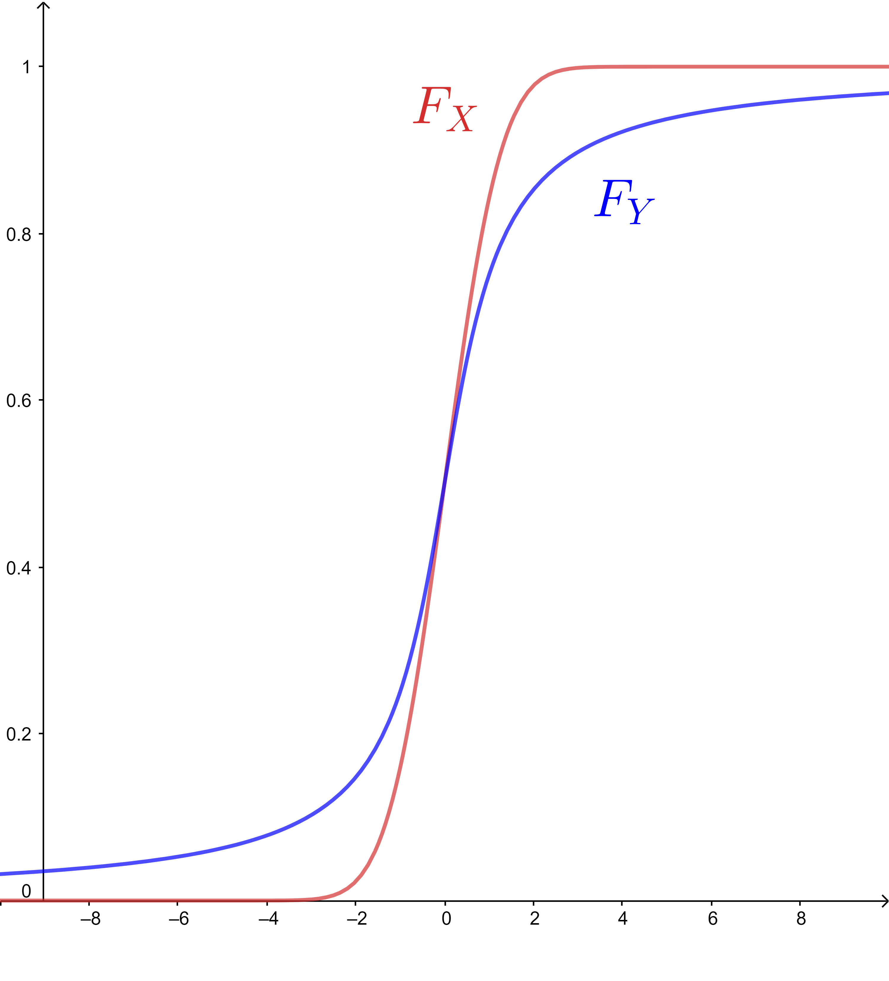
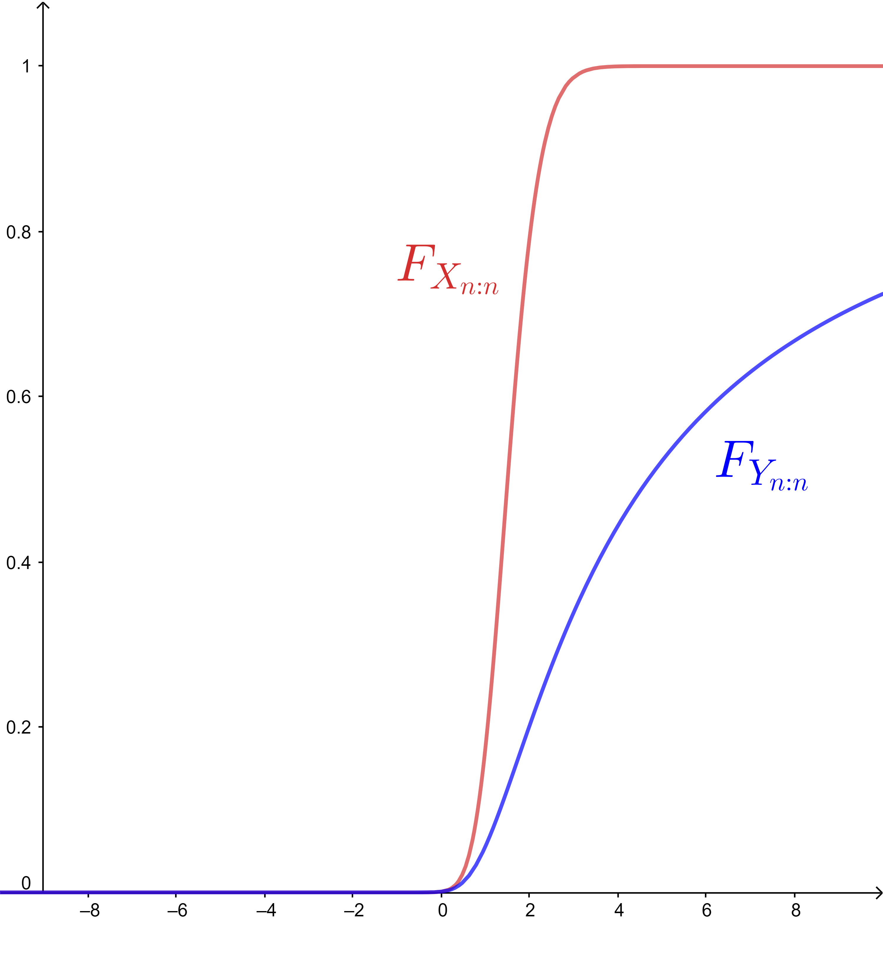
We observe that, in the region $(-\infty,0)$, i.e. where $F_{Y}$ dominates $F_{X}$ (and hence $F_{Y_{n:n}}$ dominates $F_{X_{n:n}}$), the difference between $F_{X_{n:n}}$ and $F_{Y_{n:n}}$ is almost negligible, while in the region $(0,\infty)$, where the dominance is opposite, the difference is inflated. These observations motivate us to examine stochastic dominance that may exist between $X_{n:n}$ and $Y_{n:n}$ in some asymptotic sense. We find out that this is indeed the case, according to the asymptotic stochastic orders, formulated in this work.

Throughout the paper, we stick to the following notations and conventions. For any function $f:\mathbb{R}\to\mathbb{R}$ and any set $A\subseteq\mathbb{R}$, we denote $f(A)=\{f(x):x\in A\}$. For any $x\in\mathbb{R}$ and $S\subseteq\mathbb{R}$, we denote $\textnormal{dist}\left(x,S\right)=\inf_{y\,\in\,S}\left|x-y\right|$. For an arbitrary set $T\subseteq\mathbb{R}$ which is unbounded above, the limit of a real-valued function $t\mapsto\psi(t)$ defined on $T$, as $t\to\infty$, is considered in the usual sense, i.e. $\lim_{t\to\infty}\psi(t)\equiv\lim_{t\to\infty;\,t\,\in\,T}\psi(t)=a\in\mathbb{R}\cup\left\{-\infty,\infty\right\}$ if for every sequence $\left\{t_{n}\in T:n\in\mathbb{N}\right\}$ with $t_{n}\to\infty$, as $n\to\infty$, we have $\lim_{n\to\infty}\psi(t_{n})=a$. For any real-valued function $g$, we define the left-continuous inverse by $g^{\leftarrow}(y)=\inf{\{x\in\mathbb{R}:g(x)\geqslant y\}}$ and the right-continuous inverse of $g$ by $g^{\rightarrow}(y)=\sup{\{x\in\mathbb{R}:g(x)\leqslant y\}}$. Evidently, $g^{\leftarrow}(y)\leqslant g^{\rightarrow}(y)$. We denote $g(x-)=\lim_{t\uparrow x}g(t)$ and $g(x+)=\lim_{t\downarrow x}g(t)$, when the limits exist.

The rest of the paper is structured as follows. In Section 2 and Section 3, respectively, we give the formal definitions of asymptotic usual stochastic order and asymptotic stochastic precedence order. Various properties and interrelation of these two orders are also discussed. In Section 4, the need for quantitative approach in formulating asymptotic stochastic orders is illustrated and the basis of two quantitative asymptotic stochastic orders is developed, based on $L_{1}$ and $\mathcal{W}_{2}$ distances (defined in Section 5 and Section 6, respectively) between cdfs. In Section 5 and Section 6, respectively, we define and analyze the $L_{1}$-asymptotic usual stochastic order and the $\mathcal{W}_{2}$-asymptotic usual stochastic order. Interrelation between the two orders is also shown. In Section 7, we have derived sufficient conditions for the asymptotic stochastic orders for mixtures of order statistics from samples with possibly non-integral size, as well as record values from two different homogeneous samples, as the sample size becomes large, to hold.

Let $\left\{X_{t}:t\in T\right\}$ and $\left\{Y_{t}:t\in T\right\}$ be two stochastic processes with $T\subseteq\mathbb{R}$. Throughout the paper, we shall assume the index set $T$ to be unbounded above. Note that, when $T=\mathbb{N}$ (resp. $T=[0,\infty)$), the processes become discrete-time (resp. continuous-time) stochastic processes. It is a well-known fact that $X\leqslant_{\textnormal{st}}Y$ if and only if $F_{X}^{\leftarrow}(u)\leqslant F_{Y}^{\leftarrow}(u)$, for every $u\in(0,1)$. Lehmann 1955 notes that this characterization of usual stochastic order in terms of the quantile functions is more intuitive than Section 1. Now, it may happen that there does not exist any $t\in T$ such that $X_{t}\leqslant_{\textnormal{st}}Y_{t}$ but, as $t\to\infty$, it increasingly gets closer to $X_{t}\leqslant_{\textnormal{st}}Y_{t}$, in the sense that $F_{X_{t}}^{\leftarrow}(u)\leqslant F_{Y_{t}}^{\leftarrow}(u)$ is satisfied for every $u\in(0,1)$, except for a set, whose Lebesgue measure shrinks to $0$, as $t\to\infty$. This leads to the following definition.

The next lemma shows that the condition, stated in (2.1), remains the same if any of the left-continuous inverses is changed to right-continuous inverse. The proof is straightforward and hence omitted.

If the respective distributions of $X_{t}$ and $Y_{t}$ are continuous, for every $t\in T$, then it is possible to characterize asymptotic usual stochastic order in terms of the probability measure assigned to the region of the support where $F_{X_{t}}\geqslant F_{Y_{t}}$, by both $P_{X_{t}}$ and $P_{Y_{t}}$, the probability measures induced by $F_{X_{t}}$ and $F_{Y_{t}}$, respectively. For that purpose, we need the following lemmas, the proofs of which are given in the appendix.

The next theorem shows characterization of the asymptotic usual stochastic order in terms of probability measures of the region $\{x\in\mathbb{R}:F_{X_{t}}(x)<F_{Y_{t}}(x)\}$.

The proof follows from the lemmas 2.1, 2.2 and 2.3. Next, we give a characterization of asymptotic equality in usual stochastic order in the next proposition. The proof trivially follows from Section 2 and is omitted.

The next result shows that the asymptotic usual stochastic order is a partial order.

The next theorem shows that asymptotic usual stochastic order for stochastic processes is closed under nondecreasing, continuous transformations.

The next lemma shows that asymptotic usual stochastic order is reversed by negation of stochastic processes. The proof follows from Lemma 2.1 and the observations that $F_{-X}^{\leftarrow}(u)=-F_{X}^{\rightarrow}(1-u)$ and $F_{-X}^{\rightarrow}(u)=-F_{X}^{\leftarrow}(1-u)$, for every $u\in(0,1)$, for any random variable $X$.

Observing that if $\psi$ is nonincreasing, then $-\psi$ is nondecreasing and using Lemma 2.8 we have the following corollary of Theorem 2.7.

In particular, for linear transformations of stochastic processes, we have the following result.

The next theorem shows an intuitive connection between asymptotic usual stochastic order and convergence in probability of stochastic processes to certain subsets of $\mathbb{R}$.

In the previous sections, we have explored asymptotic stochastic orders based on stochastic orders that do not consider any dependence structure between $X_{t}$ and $Y_{t}$ into account. In this section, we discuss an alternative approach based on stochastic precedence order, that considers any possible dependence structure between the two stochastic processes into account.

Note that, $X_{t}=_{\textnormal{asp}}Y_{t}$, as $t\to\infty$ if and only if $\lim_{t\to\infty}P\{X_{t}\leqslant Y_{t}\}=1/2$. The next theorem shows that, for any two independent stochastic processes, asymptotic usual stochastic order is stronger than asymptotic stochastic precedence order. We need the next lemma to prove it.

The next theorem shows that asymptotic stochastic precedence order of the stochastic processes is closed under nondecreasing transformations.

Observing that $-\psi$ is nondecreasing (resp. strictly increasing) if and only if $\psi$ is nonincreasing (resp. strictly decreasing), we immediately have the following corollary.

It follows from Theorem 3.2 that under the setup of Theorem 2.11, we have $X_{t}\leqslant_{\textnormal{asp}}Y_{t}$, as $t\to\infty$. The next theorem gives a stronger conclusion.

As defined in Section 2, $X_{t}\leqslant_{\textnormal{ast}}Y_{t}$, as $t\to\infty$ if $\lim_{t\to\infty}\mu(\{u\in(0,1):F_{X_{t}}^{\leftarrow}(u)>F_{Y_{t}}^{\leftarrow}(u)\})=0$. A limitation of this condition is that, the measure $\mu(\{u\in(0,1):F_{X_{t}}^{\leftarrow}(u)>F_{Y_{t}}^{\leftarrow}(u)\})$ considers only the sign of $F_{X_{t}}^{\leftarrow}(u)-F_{Y_{t}}^{\leftarrow}(u)$ and does not take into account the magnitude of the same. For that reason, we say that the definition is semi-quantitative in nature. As a result, $X_{t}\leqslant_{\textnormal{ast}}Y_{t}$, as $t\to\infty$ does not hold in a lot of situations where asymptotic stochastic order should hold from an intuitive point of view, as demonstrated in the following example.

References

- Ahsanullah & Nevzorov [2011] Ahsanullah, M. & Nevzorov, V. B. (2011). Record Statistics. In: International Encyclopedia of Statistical Science, Lovric, M. (Ed.). 1195–1202. Springer Berlin Heidelberg.
- Arcones et al. [2002] Arcones, M. A., Kvam, P. H., & Samaniego, F. J. (2002). Nonparametric estimation of a distribution subject to a stochastic precedence constraint. Journal of the American Statistical Association, 97(457), 170–182.
- Bergmann [1991] Bergmann, R. (1991). Stochastic orders and their application to a unified approach to various concepts of dependence and association. In: Stochastic Orders and Decision Under Risk, Mosler, K. and Scarsini, M. (Eds.), 48–73. Lecture Notes–Monograph Series, volume 19. Institute of Mathematical Statistics, Hayward, CA.
- Birnbaum [1956] Birnbaum, Z. W. (1956). On a Use of the Mann-Whitney Statistic. In: Proceedings of the Third Berkeley Symposium on Mathematical Statistics and Probability, Volume 1: Contributions to the Theory of Statistics, Neyman, J. (Ed.). 13–17. University of California Press, Berkeley, California.
- Boland et al. [2002] Boland, P. J., Hu, T., Shaked, M., & Shanthikumar, J. G. (2002). Stochastic Ordering of Order Statistics II. In: Modeling Uncertainty: An Examination of Stochastic Theory, Methods, and Applications, Dror, M., L’Ecuyer, P. and Szidarovszky, F. (Eds.), 607–623. Springer, New York.
- Bäuerle & Bayraktar [2013] Bäuerle, N. & Bayraktar, E. (2013). A note on applications of stochastic ordering to control problems in insurance and finance. Stochastics, 86(2), 330–340.
- Bäuerle & Müller [2006] Bäuerle, N. & Müller, A. (2006). Stochastic orders and risk measures: Consistency and bounds. Insurance: Mathematics and Economics, 38(1), 132 – 148.
- Chandler [1952] Chandler, K. N. (1952). The distribution and frequency of record values. Journal of the Royal Statistical Society. Series B, 14(2), 220–228.
- de la Cal & Cárcamo [2006] de la Cal, J. & Cárcamo, J. (2006). Stochastic orders and majorization of mean order statistics. Journal of Applied Probability, 43(3), 704–712.
- Denneberg [1994] Denneberg, D. (1994). Non-Additive Measure and Integral. Springer, Netherlands.
- Dziubdziela & Kopociński [1976] Dziubdziela, W. & Kopociński, B. (1976). Limiting properties of the k-th record values. Applicationes Mathematicae, 15(2), 187–190.
- Fábián et al. [2011] Fábián, C. I., Mitra, G., & Roman, D. (2011). Processing second-order stochastic dominance models using cutting-plane representations. Mathematical Programming, 130, 33–57.
- Fill & Kahn [2013] Fill, J. A. & Kahn, J. (2013). Comparison inequalities and fastest-mixing Markov chains. Annals of Applied Probability, 23(5), 1778–1816.
- Hazra et al. [2017] Hazra, N. K., Kuiti, M. R., Finkelstein, M., & Nanda, A. K. (2017). On stochastic comparisons of maximum order statistics from the location-scale family of distributions. Journal of Multivariate Analysis, 160, 31–41.
- Juan & Vidal [2002] Juan, A. & Vidal, E. (2002). On the use of Bernoulli mixture models for text classification. Pattern Recognition, 35(12), 2705–2710.
- Khaledi & Shaked [2010] Khaledi, B.-E. & Shaked, M. (2010). Stochastic comparisons of multivariate mixtures. Journal of Multivariate Analysis, 101(10), 2486 – 2498.
- Kijima & Ohnishi [1999] Kijima, M. & Ohnishi, M. (1999). Stochastic orders and their applications in financial optimization. Mathematical Methods of Operations Research, 50, 351–372.
- Kotz et al. [2003] Kotz, S., Lumelskii, Y., & Pensky, M. (2003). The Stress–Strength Model and Its Generalizations. World Scientific, Singapore.
- Lehmann [1955] Lehmann, E. L. (1955). Ordered families of distributions. Annals of Mathematical Statistics, 26(3), 399–419.
- Lopes et al. [2003] Lopes, H. F., Müller, P., & Rosner, G. L. (2003). Bayesian meta-analysis for longitudinal data models using multivariate mixture priors. Biometrics, 59(1), 66–75.
- López-Díaz et al. [2018] López-Díaz, M. C., López-Díaz, M., & Martínez-Fernández, S. (2018). A stochastic order for the analysis of investments affected by the time value of money. Insurance: Mathematics and Economics, 83, 75–82.
- McLachlan & Basford [1988] McLachlan, G. J. & Basford, K. E. (1988). Mixture Models. Inference and Applications to Clustering. Marcel Dekker, New York.
- Müller & Shaked [2013] Müller, A. & Shaked, M. (2013). Stochastic Orders for Stochastic Processes. In: Wiley Encyclopedia of Operations Research and Management Science, Cochran, J. J. (Ed.). 1–7. American Cancer Society.
- Müller & Scarsini [2006] Müller, A. & Scarsini, M. (2006). Stochastic order relations and lattices of probability measures. SIAM Journal on Optimization, 16(4), 1024–1043.
- Muller & Stoyan [2002] Muller, A. & Stoyan, D. (2002). Comparison Methods for Stochastic Models and Risks. John Wiley & Sons, New York.
- Navarro et al. [2013] Navarro, J., del Águila, Y., Sordo, M. A., & Suárez-Llorens, A. (2013). Stochastic ordering properties for systems with dependent identically distributed components. Applied Stochastic Models in Business and Industry, 29(3), 264–278.
- Panaretos & Zemel [2019] Panaretos, V. M. & Zemel, Y. (2019). Statistical Aspects of Wasserstein Distances. Annual Review of Statistics and Its Application, 6(1), 405–431.
- Pledger & Proschan [1973] Pledger, G. & Proschan, F. (1973). Stochastic comparisons of random processes, with applications in reliability. Journal of Applied Probability, 10(3), 572–585.
- Reynolds et al. [2000] Reynolds, D. A., Quatieri, T. F., & Dunn, R. B. (2000). Speaker Verification Using Adapted Gaussian Mixture Models. Digital Signal Processing, 10(1), 19–41.
- Samaniego [2007] Samaniego, F. J. (2007). System Signatures and their Applications in Engineering Reliability. Springer, New York.
- Schlattmann & Böhning [1993] Schlattmann, P. & Böhning, D. (1993). Mixture models and disease mapping. Statistics in Medicine, 12(19‐20), 1943–1950.
- Shaked & Shanthikumar [2007] Shaked, M. & Shanthikumar, J. G. (2007). Stochastic Orders. Springer, New York.
- Sordo & Suárez-Llorens [2011] Sordo, M. A. & Suárez-Llorens, A. (2011). Stochastic comparisons of distorted variability measures. Insurance: Mathematics and Economics, 49(1), 11–17.
- Stigler [1977] Stigler, S. M. (1977). Fractional order statistics, with applications. Journal of the American Statistical Association, 72(359), 544–550.
- Stoyan [2001] Stoyan, D. (2001). Comparison Methods for Queues and Other Stochastic Models. UMI Research Press, Michigan.
- Tepedelenlioglu et al. [2011] Tepedelenlioglu, C., Rajan, A., & Zhang, Y. (2011). Applications of stochastic ordering to wireless communications. IEEE Transactions on Wireless Communications, 10(12), 4249–4257.
- Wang [1995] Wang, S. (1995). Insurance pricing and increased limits ratemaking by proportional hazards transforms. Insurance: Mathematics and Economics, 17(1), 43–54.
- Wang [1996] Wang, S. (1996). Premium calculation by transforming the layer premium density. ASTIN Bulletin, 26(1), 71–92.
- Wang & Young [1998] Wang, S. & Young, V. R. (1998). Ordering risks: Expected utility theory versus Yaari’s dual theory of risk. Insurance: Mathematics and Economics, 22(2), 145–161.
- Wei [2017] Wei, W. (2017). Joint stochastic orders of high degrees and their applications in portfolio selections. Insurance: Mathematics and Economics, 76, 141–148.
9. Appendix
Proof of Lemma 2.2.