marginparsep has been altered.
topmargin has been altered.
marginparwidth has been altered.
marginparpush has been altered.
The page layout violates the ICML style.
Please do not change the page layout, or include packages like geometry, savetrees, or fullpage, which change it for you.
We’re not able to reliably undo arbitrary changes to the style. Please remove the offending package(s), or layout-changing commands and try again.
Wasserstein GANs Work Because They Fail
(to Approximate the Wasserstein Distance)
Jan Stanczuk 1 Christian Etmann 1 Lisa Maria Kreusser 2 Carola-Bibiane Schönlieb 1
Preprint.
.
Abstract
Wasserstein GANs (WGANs) are based on the idea of minimising the Wasserstein distance between a real and a generated distribution. We provide an in-depth mathematical analysis of differences between the theoretical setup and the reality of training WGANs. In this work, we gather both theoretical and empirical evidence that the WGAN loss is not a meaningful approximation of the Wasserstein distance. In addition, we argue that the Wasserstein distance is not a desirable loss function for deep generative models. We conclude that the success of WGANs can be attributed to the failure to approximate the Wasserstein distance.
1 Introduction
The Wasserstein GAN (WGAN), first introduced in (Arjovsky et al. 2017), is a framework for training Generative Adversarial Networks (GANs) by minimising the Wasserstein-1 distance (henceforth just called ‘the’ Wasserstein distance) between a real and a generated distribution. The use of the Wasserstein distance was motivated as a remedy for shortcomings of the Jensen-Shannon (JS) divergence, which is implicitly used in vanilla GANs (Goodfellow et al. 2014), but introduces some fundamental problems (Arjovsky & Bottou 2017).
Over time, practical implementations of WGANs have continuously been improved. Improvements include WGANs with gradient penalty (WGAN-GP) (Gulrajani et al. 2017) or, for specific cases only, so-called StyleGANs (Karras et al. 2018). While the generative performance of WGANs has gained wide-spread interest, other works Le et al. 2019b; Lunz et al. 2019 train WGANs specifically to employ the trained discriminators (also called critics) to estimate Wasserstein distances.
In recent years, WGANs have become one of the most studied and successful deep generative models. Initially it was suggested that the success of WGANs can be attributed to the use of the Wasserstein distance. Many publications Lei et al. 2019; Le et al. 2019a; Cho & Suh 2019; Huang et al. 2019; Erdmann et al. 2018 (including some of our own prior work Lunz et al. 2019 and educational materials Weng 2019 still propagate or even rely on the assumption that WGANs are capable of approximating the Wasserstein distance accurately and that an accurate approximation is desirable. However, the theoretical foundations of WGANs and the validity of the theoretical assumptions made in (Arjovsky et al. 2017) have received little attention so far. In the studies by Pinetz et al. 2019; Mallasto et al. 2019b, the authors examine certain failures of the approximation of the correct Wasserstein distance via WGAN-GP.
In our work, we take a critical look at the original motivation of WGANs. We explore both theoretical and practical shortcomings of WGANs, and conclude that real-world implementations of WGANs should not be thought of as Wasserstein distance minimisers. We show that certain theoretical assumptions on WGANs are not satisfied in practise and infer that aiming for an accurate approximation of the Wasserstein distance with a WGAN loss is counterproductive and leads to worse results. We argue that the original success of WGAN-GP is likely to be the result of the regularisation of the discriminator (via Lipschitz constraints) and can be regarded as a carefully-chosen hyperparameter configuration rather than as a new loss function.
We point out subtle differences between various possible notions of the ‘Wasserstein distance as a loss function’, including the ‘distributional’ Wasserstein distance and the ‘batch’ Wasserstein distance (for their definitions see Section 1.2). The batch Wasserstein distance is of interest in several works, see Mallasto et al. 2019b; Mallasto et al. 2019a; Fatras et al. 2020, where it has been examined as a potential loss function for WGAN-based generative models.
Sample complexity estimates (compare Section 5) show that estimating the true Wasserstein distance between distributions via batches requires prohibitive batch sizes. We demonstrate that even with a favourable sample complexity (obtained via entropic regularisation), the generated samples of good batch Wasserstein estimators have a low fidelity.
For the case of Bernoulli measures, minimising batch Wasserstein distances leads to noticeably different minimisers than minimising the actual Wasserstein distance between data-generating distributions (Bellemare et al. 2017). Moreover, there is a non-vanishing bias in sample estimates of the gradient of Wasserstein distances which can have an influence on gradient descent based learning algorithms. We take this analysis further and show empirically that false or undesirable minima occur not only in the case of Bernoulli measures, but also while learning common synthetic and benchmark distributions.
We show that a perfect generator – one that outputs actual samples from the data set – yields a significantly higher batch Wasserstein distance on average than a distribution concentrated on the centroids of geometric k-medians clustering. We prove that in a certain sense, these centroids comprise the batch that has the optimal Wasserstein distance to the data set.
A variant of the batch Wasserstein distance has been suggested as a loss function for a generative model in Fatras et al. 2020, but experiments are only provided for 2D Gaussian data. Based on our theory we predict that when applied to image data a model based on the batch Wasserstein distance results in blurry k-medians-like images which is also confirmed by our numerical experiments. We argue that the Wasserstein-1 distance is not a desirable loss function for deep generative models for image data due to the reliance on pixel-wise metrics, and we provide empirical evidence for this. We conclude that the success of WGANs can be attributed to the failure to approximate the Wasserstein distance.
While Mallasto et al. 2019b suggests using the -transform as a more accurate batch Wasserstein estimator, a worse generative performance has been observed. We demonstrate that the drop in performance is related to sample complexity and optimisation, but is also an issue of the Wasserstein distance itself due to the euclidean distance as the underlying metric.
This analysis raises a natural question: If models like WGAN-GP (which generate high-fidelity samples) do not use a meaningful approximation of the Wasserstein distance, why do they achieve said visual performance, often better than the vanilla GAN (Goodfellow et al. 2014)? The literature suggests two possible answers: Firstly, it has been proposed in (Kodali et al. 2017) and (Fedus et al. 2017) that regularising the Lipschitz constraint of the discriminator may improve stability of GAN training regardless of the statistical distance used as a loss function. Secondly, in (Lucic et al. 2017), a large-scale experiment has shown that vanilla GANs can achieve similar performance to WGAN-GP if the right hyperparameters are chosen. Therefore, the original success of WGAN-GP might be due to a carefully-chosen hyperparameter configuration rather than because of the new loss function. Our observations agree with the points made in (Fedus et al. 2017) that GANs should not be understood as minimisers of some statistical distance. This suggests that the dynamics of the optimisation process based on alternating gradient updates need to be understood better and it is not sufficient to study the loss function or the optimal discriminator regime.
1.1 Contributions
The contributions of our work are as follows:
- 1.
We provide a careful in-depth discussion on the modelling assumptions in (Arjovsky et al. 2017). We specify the different ways in which the training of WGANs can (and in practice, does) fail to approximate Wasserstein distance estimators and we demonstrate these claims by providing theoretical and empirical evidence.
- 2.
We point out subtle differences between various possible notions of the ‘Wasserstein distance as a loss function’. We show that for the batch Wasserstein distance, sample complexity issues fail to fully explain the failure (first noted by (Mallasto et al. 2019b)) of good batch Wasserstein estimators to generate high-fidelity samples.
- 3.
In addition to known results in (Bellemare et al. 2017), we demonstrate that the batch Wasserstein-1 distance is not even a desirable loss function for GANs. For this, we derive a new connection between the Wasserstein distance and clustering (geometric -medians clustering), which results in undesirable, low-fidelity samples, that nevertheless exhibit a low Wasserstein distance. We provide an experiment which shows that on the contrary, even a perfect generator (outputting actual data samples) yields a comparatively large Wasserstein distance.
- 4.
We argue that the fundamental problems of the Wasserstein-1 distance stem from the underlying euclidean metric. We suggest that the failure to approximate the Wasserstein distance accurately enables the generation of high-fidelity samples. In fact, the regularisation of the discriminator (in WGANs motivated by a Lipschitz constraint on the discriminator) helps generate good-looking samples, even when non-Wasserstein GANs are used.
1.2 Notation
In this work, we use the following notation.
- •
Empirical measures: Given a probability distribution , we denote the empirical measure of samples by , defined by , where for are independent and identically distributed (i.i.d.) samples from . Thus, represents a mini-batch of samples from and we can consider as a distribution. We write if is distributed according to . The expectation of a given function satisfies .
- •
Set of empirical measures: Given a probability distribution , we denote the set of all empirical measures of samples drawn from by . We write if we draw an empirical measure from the set .
- •
Lipschitz continuity: For a Lipschitz continuous function , we denote its Lipschitz constant with respect to the euclidean norm (both in the domain and co-domain) by .
- •
Wasserstein distance: The Wasserstein distance is defined as
(1.1) where the infimum is taken over all joint distributions with marginals and . The above is referred to as the primal formulation of Wasserstein distance. The Kantorovich-Rubenstein duality is given by
(1.2) This is referred to as the dual formulation. The maximiser is called Kantorovich’s potential between and and is determined (up to a constant) by and .
- •
Oracle estimator: Let the empirical measures associated with the probability distributions be given. We define the oracle estimator as
where
(1.3) is Kantorovich’s potential.
- •
Mini-batch estimator: Given empirical measures , we define the mini-batch estimator as
- •
Batch Wasserstein and distributional Wasserstein distance: Sometimes we wish to emphasise the difference between and . In such cases we refer to the former as batch Wasserstein distance and to the latter as distributional Wasserstein distance.
1.3 Outline
This paper is structured as follows. In Section 2, we give an overview on the original theory motivating the introduction of WGANs. In Section 3, we discuss how the Wasserstein distance is approximated in WGANs and distinguish two notions of Wasserstein distance as a loss function in the literature: the batch Wasserstein distance between mini-baches and the distributional Wasserstein distance. We examine how well different WGANs approximate the loss function in Section 4. We conclude that WGANs fail to approximate the distributional Wasserstein distance and that a better approximation of the Wasserstein distance between minibatches leads to worse generative performance. In Section 5, we explore how sample complexity makes the efficient approximation of distributional Wasserstein distance impossible. We further investigate false minima of the batch Wasserstein distance and their connection to clustering. In section 6, we discuss fundamental issues of the Wasserstein distance as a loss function for image data stemming from the fact that it is based on the pixelwise distance. In section 7, we discuss possible explanations for the initially reported success of WGAN in light of the failure to approximate Wasserstein distance.
2 Original Motivations for Wasserstein GAN
2.1 Theoretical formulation of GANs
Generative adversarial networks (GANs) were introduced in (Goodfellow et al. 2014) as a new framework for generative models. A GAN consists of two neural networks: the generator and the discriminator which compete against each other. Here, denotes the latent space, is the data space and denote the parameters of the respective networks. The space is usually endowed with a multivariate Gaussian distribution . For with , the outputs of the generator form a distribution which we call the generator distribution and denote by . The generator learns to produce samples which resemble the data from a target distribution , while the discriminator is trying to distinguish fake from real data (by assigning an estimated probability that is ‘real’ rather than generated data). In the context of WGANs, the discriminator is often called ‘critic’. Hence, we train to maximize the probability of assigning the correct label to both training examples and samples from , while we train to minimise the discrepancy between the generated samples and data. Formally, given a value function the optimisation objective is of the form
2.2 Optimal discriminator dynamics
A common approach to analysing the training of GANs is the so-called optimal discriminator dynamics. In the optimal discriminator dynamics approach, we define and analyse GANs as a minimisation problem (rather than a mini-max problem):
This approach to modelling GAN dynamics relies on what we call the optimal discriminator assumption (ODA), i.e. that after each update of the generator, we assume that the best possible discriminator was picked. This is not the case in practice, as we will discuss in later sections.
If we choose the right value function, we can interpret GAN training as a minimisation of a statistical divergence between a target and a generated distribution under the ODA. For example in (Goodfellow et al. 2014), it has been shown that vanilla GAN’s value function
induces the minimisation of the Jensen-Shannon divergence
between the real distribution and the generator distribution where denotes the Kullback-Leibler divergence.
2.3 Choosing the right divergence
A rigorous mathematical analysis of the vanilla GAN’s optimal discriminator dynamics has been performed in (Arjovsky & Bottou 2017). The authors prove that for the vanilla GAN’s value function, an accurate approximation of the optimal discriminator leads to vanishing gradients passed to the generator (i.e. as approaches the optimal discriminator ). This problem can be traced back to the fact that the JS divergence is maximised whenever two distributions have disjoint supports. To address this issue, the authors in Arjovsky et al. 2017 suggest to replace the JS divergence by the Wasserstein distance which decreases smoothly as the supports of the distributions converge to each other. In order to apply the Wasserstein distance to GAN training, the authors use the Kantorovich-Rubenstein duality (1.2) and redefine the GAN objective function as
| (2.1) |
The mini-max objective can be rewritten as
| (2.2) |
which shows that the 1-Lipschitz functions act as the class of possible discriminators.
3 Estimation of in WGANs
3.1 WGAN-GP Algorithm
The exact computation of
| (3.1) |
is in practice impossible for two reasons. Firstly, it is computationally impossible to optimise over the set of all 1-Lipschitz functions accurately. Secondly, we do not have access to the full measures and , but only to finite samples from each of them. Therefore, the Wasserstein distance has to be approximated via some tractable loss function in WGANs. There are many suggestions for loss functions in the literature (e.g. (Arjovsky et al. 2017; Gulrajani et al. 2017; Miyato et al. 2018)). We focus on the most prominent approximation scheme, introduced in Gulrajani et al. 2017. The function in the duality formula (3.1) is replaced by a neural network , which is then trained to maximise (3.1). Moreover the network is (at least approximately) constrained to be a 1-Lipschitz function. For this reason a regularisation term called gradient penalty is incorporated in the loss function. More precisely, let and denote the empirical measures associated with measures and for the samples and , respectively. Define
| (3.2) | ||||
| (3.3) |
where is defined as the uniform distribution on the lines connecting with for . Note that (3.2) can be regarded as an approximation of (2.1), while (3.3) enforces the gradient penalty.
Then one can optimise an approximation of the mini-max objective in (2.2) in an iterative fashion. First sample batches and make a gradient ascent step with respect to the discriminator loss function . Repeat this process times (to approximate ). Then sample new batches and make a gradient descent step with respect to the generator loss . Repeat the whole procedure times. The WGAN-GP is described in pseudo-code in the Algorithm 1.
Remark 1.
In (3.2) we use a different notation for the value function instead of in (2.1). First notice that in (2.1) depends on only through and hence we may regard as a function of and . Sometimes we want to refer explicitly to the value function evaluated using randomly sampled mini-batches and . In this case we shall write as in (3.2).
Remark 2.
In Algorithm 1 we could have removed the second sampling from and descent wrt. instead of . This would result in the same minimiser , but in such case would not approximate .
3.2 c-transform WGAN
An approximation scheme based on -transform has been proposed in Mallasto et al. 2019b which gives a more accurate approximation of between mini-batches than WGAN-GP. The main idea of their approach is to replace the Kantorovich-Rubenstein duality with the following so-called weak duality formula:
Theorem 3.2.1 (Weak Duality, Mallasto et al. 2019b).
For probability distributions , we have
where the supremum is taken over the space of all continuous bounded functions such that satisfies and is its c-transform of .
Note that the -transform of a 1-Lipschitz function is given by . Hence, is easy to compute for 1-Lipschitz functions. However, note that the optimisation is over the space of .
In the -transform WGAN, the authors use the weak duality (Theorem 3.2.1) instead of Kantorovich-Rubinstein duality. This allows for the optimisation of the discriminator to be unconstrained, but introduces an approximate -transform in the objective which reads
The mini-max objective can be rewritten as
Similarly to the WGAN-GP in Section 3, we consider the loss approximation
| (3.4) |
where is an approximation to -transform of given as .
3.3 The oracle estimator
The main idea behind the WGAN-GP algorithm is that , optimised in the inner loop, approximates Kantorovich’s potential between and in (1.3). As a result the loss function of the generator approximates the oracle estimator of the Wasserstein distance
where
From the above discussion, we can conclude that there are two sources of error in the approximation of the Wasserstein distance:
- 1.
Not learning the optimal discriminator exactly.
- 2.
Estimation of the expectations based on finite samples.
We discuss the impact of each source of error in the following sections. Moreover, we notice that even if we approximate the Wasserstein distance perfectly we still need to perform a non-convex optimisation via a stochastic gradient descent based learning algorithm on in order to successfully train a GAN.
3.4 The batch estimator
Recently, some researchers have examined how well the loss function of WGAN approximates the distance between random mini-batches Mallasto et al. 2019b. More precisely, instead of approximating the oracle estimator they suggest that the loss function of WGAN should approximate the batch estimator
Here we have following sources of error:
- 1.
Not learning the optimal discriminator exactly.
- 2.
Fitting the discriminator to and instead of and (sample complexity).
Using Theorem 3.2.1, the batch estimator can be written as
4 Approximation of the optimal discriminator
In the following, we discuss how accurately the optimal discriminator is approximated in the different methods for the estimation of the Wasserstein distance. In other words, we investigate whether the loss function of WGAN-GP satisfies the approximations and . This question has been explored in two recent works by Mallasto et al. 2019b and Pinetz et al. 2019, but our experiments differ significantly. The subtle, but crucial differences are explained in detail in the Appendix B.
We show the following relations which are summarised in Figure 1:
- •
- •
The loss function can approximate the batch estimator when trained using the -transform, but is not a good approximation of the distribution level Wasserstein distance (Section 4.2).
- •
The batch estimator of the Wasserstein distance is not a desirable loss function for a generative model (Section 5).
- •
The close connection of the Wasserstein distance to the pixelwise norm causes fundamental issues when applying the Wasserstein distance to image data (Section 6).

4.1 Approximation of the oracle estimator
First, we examine whether
| (4.1) |
is a valid approximation. This is the case if and only if the inner loop of the WGAN-GP algorithm 1, also called the discriminator loop, computes a good approximation of Kantorovich’s potential in (1.3).
4.1.1 Approximation for fixed, finitely supported distributions
To examine whether (4.1) is satisfied in practice, we design the following experiment, summarised in Algorithm 2. We pick two large finitely supported distributions and , each consisting of K images from CIFAR-10 Krizhevsky 2009. Then we sample mini-batches (of size ) from and maximise . This is exactly the same procedure as in the WGAN-GP training in Algorithm 1 except that both measures are static (as if the generator in Algorithm 1 was frozen). We consider updates for . At the end, we check if the approximation
is close to . Note that we return and not for in case the Lipschitz penality is not well satisfied.
Since the distributions are finitely supported, can be obtained by solving a linear program (LP) as in Flamary et al. 2021. Note that superficially similar experiment to Algorithm 2 have been performed in (Pinetz et al. 2019) and Mallasto et al. 2019b. Subtle, but crucial differences in the design of the experiment are discussed in Appendix B.
Notice that if then . Therefore we can assess the quality of the approximation of the optimal discriminator in WGAN-GP by examining how much differs from .
Remark 3.
As pointed out in Arjovsky et al. 2017 if we optimise over the set of -Lipschitz functions instead of the set of -Lipschitz functions, then the estimate of Wasserstein distance scales by the same factor, i.e.
Since the 1-Lipschitz continuity of is only approximately enforced in WGAN-GP, a normalisation by the Lipschitz constant of should be considered. We define the lower bound of by and consider the normalised Wasserstein estimate as . This normalised quantity should be compared with .
In the experiments in Figures 2 and 3, we use Algorithm 2. We find that normalised Wasserstein estimate is very far from the actual . Since , the normalised Wasserstein estimate is one order of magnitude smaller than . In the experiments in Figure 2 we explored a range of hyperparameters (, batch size, learning rate, network architecture). For the experiments visualized in Figure 3 we use the hyperparameters recommended in the original WGAN-GP paper Gulrajani et al. 2017 except for the parameter which we allowed to vary. This allows us to explore how the value of influences the Lipschitz constraint and how it impacts the quality of Wasserstein estimation.


We emphasise that the task of estimating in Algorithm 2 is easier than estimating during WGAN training. Distributions and are static, while changes after each updates to the discriminator in Algorithm 1. During WGAN training typically , while we allowed to be trained for iterations on the same pair of distributions. The fact that even this simpler task cannot be accomplished implies that the approximation of the Wasserstein distance during WGAN training is unrealistic with WGAN-GP algorithm 1.
We point out that we are conservative in our approach to normalize the Wasserstein estimate since
where the first inequality follows from , and the second inequality is supported by Figure 3.
We conclude that is not achieved in WGAN-GP, so the loss of WGAN-GP is not an accurate approximation of Wasserstein distance.
4.1.2 Approximation during training in low dimensions
In this section, we investigate whether can be achieved for the special case of low dimensions where sample complexity issues (discussed in detail in Section 5) can be neglected. In low dimensions, we can approximate accurately by for a sufficiently large number of samples (we used for this experiment). Since are finite measures, we can determine by solving the linear program and we can check how close is to during a WGAN training.
We conduct an experiment where we fit the WGAN-GP in Algorithm 1 to an 8-mode Gaussian mixture and track at each iteration. As discussed in Remark 3 we normalize the loss by as the Lipschitz constraints in WGAN-GP are only approximated. In Figure 5, we show samples from and . The associated Wasserstein distance and the normalised Wasserstein estimate obtained with Algorithm 1 are shown in Figure 5. We observe that the normalised loss is an order of magnitude smaller the as in the Experiments in Section 4.1.1. Notice that any sensible positive loss function will be close to zero. Again we conclude that even in a simple two dimensional case is not achieved.


4.2 Approximation of the batch estimator
In this section we examine whether
We consider two algorithms: WGAN-GP Gulrajani et al. 2017 and c-transform WGAN Mallasto et al. 2019b. We reproduce the experiment of Mallasto et al. 2019b in a higher resolution setup and we use an improved architecture. For experiments in this section, we use the architecture based on StyleGAN Karras et al. 2018 and CelebA data set Liu et al. 2015.
As in Mallasto et al. 2019b, we train WGAN according Algortihm 1. At the end of each iteration of the generator loop we solve the linear program to evaluate the true Wasserstein distance between the generated batch and the batch of the real data . Then we compare the result with . For -transform WGAN is computed using the equation 3.4.
A detailed description of the experiment is included as Algorithm 3.
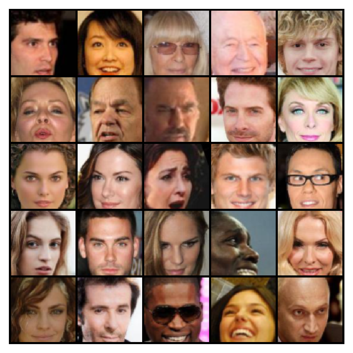
As shown in Figure 6, the gradient penalty the gradient penatly method does not provied an accurate approximation of . On the other hand, the -transform method approximates very accurately. Surprisingly, a good approximation of the batch Wasserstein distance does not correspond to a good generative performance. Figure 7 shows samples obtained from training with the -transform and the gradient penalty as the approximation method. The faces generated by a WGAN using the -transform approximation look very blurry, while the WGAN-GP results look realistic. In particular, the images obtained with WGAN using the -transform do not capture the complexity of the data set as well as WGAN-GP, despite achieving a better approximation of the Wasserstein distance. Moreover the loss function of WGAN-GP doesn’t decrease despite the samples getting better with more training. This is because the loss of WGAN-GP reflects how well the generator performs compared to the discriminator, not the Wasserstein distance.
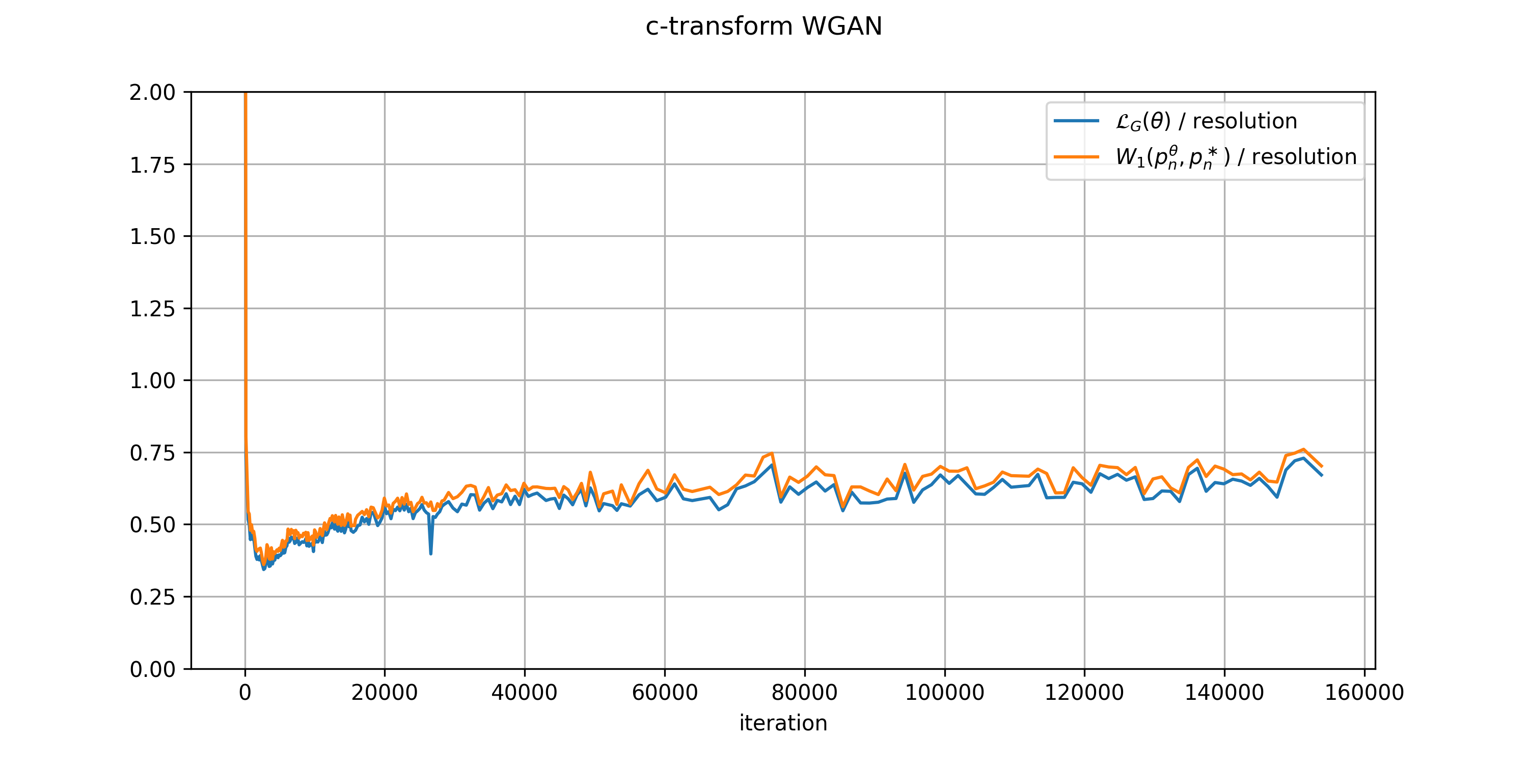


So we are left with a puzzling question: Why does a better approximation of the batch Wasserstein distance result in a worse generative performance?
In next sections, we examine possible explanations based on sample complexity, biased gradients and connections of to the -norm and clustering.
5 Finite sample approximation of
In the following, we analyse problems arising from the fact that we use finite data and minibatch-based optimisation to estimate the Wasserstein distance between high dimensional distributions.
5.1 Sample complexity of Wasserstein distance estimators
Recall that the oracle estimator is defined as
where
In the oracle estimator, the only effect of finite samples is the Monte Carlo approximation of the expectations which has a convergence rate of when samples are considered for . The oracle estimator assumes that we have access to an oracle which provides us with Kantorovich’s potential between and . Therefore, the true sample complexity is moved to the oracle and the above convergence rate is misleading. An efficient oracle does not exist and in practice, one needs huge number of samples to be able to accurately estimate .
For the batch estimator
we have and the sample complexity is well known. As shown in (Weed & Bach 2017), for -dimensional data, the expected error of the estimation of the Wasserstein distance decreases as , i.e.
where and denote the sets of all empirical measures of samples drawn from and , respectively. This decay rate is very slow in high dimensions, and hence, even if the optimal discriminator between and is learned perfectly, the loss function of WGAN is very far away from the actual Wasserstein distance.
In the following sections, we argue that sample complexity issues render the oracle estimator unrealistic and the mini-batch estimator useless.
5.2 Empirical study of sample complexity issues
In this empirical study, we illustrate that the sample size necessary for an accurate Wasserstein approximation is infeasible in the setting of high dimensional deep generative modelling. To this aim, we examine the difference between and numerically where is a standard Gaussian measure in dimensions, and are empirical measures of samples drawn from . Note that decreases to 0 as and the convergence is .
The sample Wasserstein distance concentrates very well around its expectation Weed & Bach 2017. Therefore, the behaviour of the random variable can be understood by examining
where denotes the set of all empirical measures of samples drawn from .
According to the manifold hypothesis Narayanan & Mitter 2010 the distribution which we want to learn is concentrated around a lower dimensional manifold . According to results in Weed & Bach 2017 the dimension of , known as the intrinsic dimension of , is relevant for the sample complexity of the Wasserstein distance and may be smaller than the dimension of the ambient Euclidean space. The dimension of the manifold modeled by a GAN is at most the dimension of its latent space Arjovsky & Bottou 2017. Therefore, ideally we want to set the dimension of to match the dimension of , although, when training GANs in practice, the dimension of is often set to or more Radford et al. 2016; Karras et al. 2018.
Recent research on the intrinsic dimension suggests that benchmark data sets like CIFAR-10 and CelebA could have an intrinsic dimension of around Pope et al. 2021. To illustrate that the sample size necessary for an accurate Wasserstein approximation is infeasible for high-dimensional deep generative modelling, we examine the case of for the Wasserstein distance between two random samples from the standard Gaussian distribution in Figure 8. In our experiments, we sample pairs of batches , for from and calculate the corresponding Wasserstein distance . Then we use a standard Monte Carlo estimator to approximate . Even for very large batches (up to 10,000) and for a simple Gaussian distribution, the estimation of the true Wasserstein distance (=0) is extremely bad.


Using the fact that in log-log space the relationship is linear, we fit a least squares line and extrapolate for larger values of in Figure 9. In this way we establish that in order to bring the approximation error to one would need over samples, which is much larger than any conceivable data set. In order to bring the error down to one would need over samples.

5.3 False minima of the batch Wasserstein distance
Given a target distribution and generated distribution with parameter , the difference between the true Wasserstein distance and its sample estimate may cause the existence of ‘false’ global optima, i.e. may be different from , where and denote the sets of all empirical measures of samples drawn from and , respectively.
An example of this phenomenon has already been pointed out in (Bellemare et al. 2017). The authors demonstrate that false global minima may appear when one tries to learn a Bernoulli measure by minimising the batch Wasserstein distance. For the target Bernoulli measure and the generated Bernoulli measure with parameter , they show that the sample estimate of the Wasserstein gradient is a biased estimator of . These estimation errors can strongly affect the training via stochastic gradient descent (SGD) or SGD-based algorithms like Adam. Their results are summarised in the following theorem:
Theorem 5.3.1.
- 1.
Non-vanishing mini-max bias of the sample gradient. For any there exists a pair of Bernoulli distributions , such that
- 2.
Wrong minimum of the batch Wasserstein loss. For Bernoulli measures , the minimum of the expected sample loss
is in general different from the minimum of the true Wasserstein loss .
While Theorem 5.3.1 shows that minima of the distributional and the batch Wasserstein distance may not coincide, we investigate the existence of ‘false’ minima of the batch Wasserstein distance further in the context of WGAN training and show empirically that false minima can appear while learning synthetic (e.g. Gaussian) and benchmark distributions (e.g. CelebA (Liu et al. 2015)). For this, we consider certain fixed batches (a ‘real batch’ , a ‘mean batch’ and a ‘geometric -medians batch’ ). We show empirically that in sufficiently high dimensions the expected Wasserstein distance between these batches and is largest for , even though are both empirical measures with samples drawn from and . This is achieved by approximating the expectation with the standard Monte Carlo estimator using 100 sample batches from . We conclude that a ‘mean batch’ or a ‘geometric -medians batch’ provide false minima in the case of the CelebA data set.
The results of the above experiment are visualised in the Figure 10 for CelebA. We show that the expected batch Wasserstein distance between two samples from the target distribution is greater than the expected batch Wasserstein distance between a sample from the target distribution and a sample consisting of repeated means (or geometric -medians). Therefore, a perfect generator producing samples from the target distribution would have (on average) a greater loss than a generator which learned a Dirac distribution concentrated at the mean of . Hence, the batch Wasserstein distance can push the generator towards false minima making it an undesirable loss function.
Next we compare and for the case where is the standard Gaussian distribution and is a Dirac distribution concentrated at its mean, as a function of dimension . As before, the expectation is approximated with the standard Monte Carlo estimator using 100 sample batches from . The results are visualized on Figure 11. Again we observe that in sufficiently high dimension () we have . Therefore as in the case of the CelebA dataset, a generator producing samples from the target Gaussian distribution has (on average) a greater batch Wasserstein loss than a generator which learned a Dirac distribution concentrated at the mean of in high dimensions.


5.4 Connection to clustering
As we pointed out in Section 4.2, training a WGAN using the -transform results in a better approximation of the batch Wasserstein distance, but achieves much worse generative performance than WGAN-GP. Moreover, as one can observe in Figure 12, the output of the -transform WGAN looks very similar to geometric -medians clustering.

As discussed in Section 5.2, clustering may provide samples of low batch Wasserstein distance with low visual fidelity. (Canas & Rosasco 2012) show a connection between -medians clustering and the Wasserstein-2 distance. Here, we extend these results to the Wasserstein-1 distance , which is the basis for Wasserstein GANs. Our result establishes a connection between to and geometric -medians clustering.
The well-known -means clustering determines cluster centroids so that the sum of the squared euclidean distances of the cluster elements to their respective centroid is minimal. Suppose we are given a finite set . Given an arbitrary set , let , i.e. consists of points in for which the closest point in is . K-means is the solution to the optimisation problem
If we replace the squared euclidean distance by the (unsquared) euclidean distances, we obtain geometric -medians clustering, given by
Note that for an arbitrary finite subset of an euclidean space
is called the geometric median of . Unlike in the case of squared distances (where the arithmetic mean provides the respective minimiser), iterative algorithms have to be used for computing the geometric median of a set. In this work, we use Weiszfeld’s algorithm (Weiszfeld 1937) to calculate the geometric median.
As for -means clustering, finding the true, globally optimal clustering is infeasible in practice due to the NP-hardness of the problem. We employ the standard LLoyd’s algorithm (Lloyd 1982) for clustering, which is a popular choice for -means clustering. In contrast to -means clustering (where centroids are computed via the arithmetic mean), we use Weiszfeld’s algorithm to compute the centroids, which lie in the geometric medians of the individual clusters. We initialise our clustering method with the -means clustering method in scikit-learn (Pedregosa et al. 2011), as we noticed that the geometric medians lie quite close to the arithmetic means in practice. We used 100 different random initialisations for the -means clustering to find the best loss for the geometric -medians clustering.
Let be an empirical measure formed by geometric -medians centroids. Similarly to the results for the Wasserstein-2 distance (Canas & Rosasco 2012), we show that in fact
in Theorem A.1.3. This means that the distribution concentrated at the centroids of geometric -medians has the smallest distance from the target distribution among all distributions supported on points.
This result could shed some light on why geometric -medians clustering creates undesirable minima for the batch Wasserstein distance. Training data comes in mini-batches and if we set the mini-batch size as , then the batch consisting of geometric -medians centroids is the mini-batch with the smallest possible loss.
There are still some differences between this analysis and the actual WGAN training which is based on the batch Wasserstein distance. We use a sample from the target measure, rather than the full target measure . Hence, when using batch estimator as loss, we actually minimise
wrt. . We leave the problem of formally extending Theorem A.1.3 as a possible objective for further study. We notice that in Section 5.3 we have already seen empirically (in the case of CelebA) that , where are two empirical measures, each formed by i.i.d. samples from .
6 Fundamental issues of the Wasserstein distance with image data
In the previous sections, we have argued several ways, in which WGANs may fail to learn the Wasserstein distance.
- •
In Section 4.1, we saw that WGANs used in practice distinctly fail to approximate the true oracle discriminator , i.e. they fail to minimise the distributional Wasserstein distance.
- •
In Section 4.2, we saw that WGANs with gradient penalties distinctly fail to approximate the batch Wasserstein distance.
- •
As elaborated in Sections 5.1 and 5.2, (batch) Wasserstein estimators require larger data sets than feasible in practice in order to accurately approximate the distributional Wasserstein distance. We further saw that batch Wasserstein estimators may yield false (Section 5.3) or undesirable (Section 5.4) minima.
In this section, we will show that even if some of these problems are mitigated, the resulting generators will produce undesirable images. This observation is based on the fact that the euclidean metric, i.e. the -distance based on pixelwise differences, is used explicitly in the primal formulation of the Wasserstein distance in (1.1) and implicitly in its dual formulation (1.2). We make the following conjecture: The use of the euclidean metric in the definition of the Wasserstein distance (1.1)–(1.2) is fundamentally unsuited for image data in the context of generative models.
6.1 Mitigation of sample complexity issues
In the following, let be the regularized Wasserstein distance introduced by (Cuturi 2013)
where the infimum is taken over all joint distributions with marginals and , denotes the product measure and KL is the Kullback-Leibler divergence.
Since , following (Genevay et al. 2017), we use the Sinkhorn divergence defined as
which is a normalized version of satisfying .
For , converges to the Wasserstein distance, whereas for , it converges to the maximum mean discrepancy (MMD) (Feydy et al. 2018). Since the MMD is insensitive to the curse of dimensionality (Genevay et al. 2019), the Sinkhorn divergence can be viewed as an approximation of the Wasserstein distance, which does not suffer from sample complexity issues. In particular, asymptotically as , we have
where are batches of size from , respectively.

To visualize the effect on regularisation on sample complexity,we repeat the experiments from Section 5.2. The setup is exactly the same as before, except we use Sinkhorn divergence with regularisation parameter instead of the Wasserstain distance. We compute the Sinkhorn divergence between the sample batches using the Sinkhorn iterations Cuturi 2013. The results are visualized in Figure 13. We can see that for sample size the value of expected Sinkhorn divergence is already close to 0 (contrary to what we have seen with Wasserstein distance in Section 5.2).
In (Mallasto et al. 2019b), a method for the estimation of batch Sinkhorn distances during GAN training was introduced, which is called the -transform. Surprisingly, even for high values of and thus despite a better sample complexity, the generative performance remains poor (as already noticed by (Mallasto et al. 2019b)). The generator converges to a geometric -medians-like distribution. The outputs, obtained in the same way as in Section 4.2, except that we replace the -transform by the -transform, are visualised in Figure 14. This demonstrates that mitigating sample complexity issues does not solve the problems with WGANs.

6.2 Mitigation of discriminator suboptimality issues
If we want to use the batch Wasserstein distance or Sinkhorn divergence as a loss for a generative model, we may take advantage of the fact that computation of Sinkhorn divergence admits automatic differentiation Genevay et al. 2017. Therefore we may replace the learnable discriminator by the true batch Sinkhorn distance and still compute the gradients using backpropagation. Moreover for small values of the regularization parameter this will provide a faithful approximation of the Wasserstein distance Feydy et al. 2018. Such framework has been examined in (Fatras et al. 2020). The authors suggest to minimise
wrt. , where the expectation is estimated using mini-batches sampled from and .
We emphasise that is computed exactly for each mini-batch using the Sinkhorn algorithm Cuturi 2013 instead of considering the approximation of the Sinkhorn distance in the discriminator loop as in the -transform WGAN.
We notice that this algorithm is equivalent to training a WGAN, where the discriminator optimisation step, i.e. the inner loop in Algorithm 1, is replaced by the true batch Sinkhorn distance. For sufficiently low values of we obtain a very good approximation of the optimal discriminator dynamics of batch Wasserstein GANs where the discriminator is trained to optimality for each generator update.
The authors in (Fatras et al. 2020) showed that the algorithm is successful in learning 2D euclidean data (8-mode Gaussian mixture), but they did not perform any experiments with image data. Motivated by the failure of batch Wasserstein based losses and the connection to geometric -medians described in the previous sections, we trained their model on image data. The result of the generator for CelebA is shown in Figure 15. Like for the -transform, the -transform and geometric -medians clustering which all result in low batch Wasserstein distances, we obtain non-diverse, blurry images. This demonstrates that mitigating discriminator suboptimality issues does not solve the problems with WGANs.


6.3 Fundamental failures of the -distance as a perceptual distance
Why does a Wasserstein-like distance not produce satisfactory images, even if issues related to sample complexity and suboptimality of the discriminator are mitigated? Our hypothesis is that this is due to the fact that the Wasserstein distance (and the Sinkhorn divergence) between batches of images is based on the -pixelwise distance between images. Similar conjecture has been made in Chen et al. 2019. This can be seen from the primal formulation (1.1) of (in contrast to the dual Kantorovich-Rubenstein formulation (1.2)).
For finite point clouds , we can represent them represented as a list of points and a list of probabilities for each point and allows to write (1.1) as
by (Peyré & Cuturi 2020). Here, denote the entries of the matrix , is the -th image in and is -th image in . is such that is the probability mass at and is such that is the probability mass at .
When and both have supports of size , the Wasserstein distance satisfies
where the minimisation is considered over all permutations .
When optimising the batch Wasserstein distance in the context of WGANs, we consider batches of size , drawn from the target and generated probability densities , respectively. Then, the Wasserstein distance between two batches and is the sum of pixel-wise -distances, after the images in one of the batches are permuted.
In terms of the -distance, two images tend to be similar to one another, when the brightness values of their colour channels are similar. This does not necessarily meet our human perception of two images being similar. For example, while the same person photographed under different lighting conditions would be assigned a low distance by a perceptual ‘human metric’, pixelwise metrics would consider them dissimilar (which is also a reason for the specific centroids found in geometric -medians clustering, cf. Figure 10). Wasserstein metrics on a space of distributions which are computed using pixelwise metrics on the respective sample space thus always exhibit this phenomenon. Examples of failures of the euclidean metric to capture perceptual and semantic distances between images are shown in Figure 16. We gather absurd examples, which have a lower euclidean distance to some reference image than an image, which a human would consider only a slight variation of the reference image.
Moreover, since the Wasserstein distance and the Sinkhorn divergence are metrics based on pixelwise comparisons they disregard inductive bias encoded in convolutional neural networks, which captures spatial structure present in the image data. This inductive bias is essential for the success of deep learning models Mitchell 2017, Cohen & Shashua 2017, Ulyanov et al. 2020. In fact, in our experiments we observed that methods based on accurate approximation of the batch Wasserstein distance perform similarly regardless of training with fully-connected or convolutional architectures.

A possible explanation why WGAN-GP (and in fact other GANs) produce high-fidelity samples is precisely because they do not approximate any statistical divergence which is based on pixelwise metrics. Contrary to those, the training dynamics lead to a discriminator which captures the similarity and dissimilarity between samples better, since they are more flexible than the simple model of pixelwise distances.
7 WGAN-GP in the space of GANs
In the previous sections, we established that the loss function of WGAN-GP does not approximate the Wasserstein distance in any meaningful sense. Moreover, accurate approximations of the Wasserstein distance are not even desirable in minbatch-based training in the typical high-dimensional setup. This leads to a natural question: Why does WGAN-GP achieve such a good performance? There are two possible answers in the literature which will be discussed in the following.
7.1 Lipschitz regularisation
It was suggested in (Kodali et al. 2017) and (Fedus et al. 2017) that controlling the Lipschitz constant of the discriminator may improve GAN training regardless of the statistical distance used, and that the improved performance observed in WGAN-GP was simply due to the gradient penalty term and not connected to the Wasserstein distance.
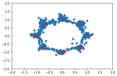
Using the architectures described in (Anil et al. 2018), we trained a WGAN and a vanilla GAN Goodfellow et al. 2014 with a multi-layer perceptron discriminator which is provably a 1-Lipschitz function. We compared this with vanilla GAN and WGAN-GP with an ordinary unconstrained multi-layer perceptron (MLP). In both cases, we observe an improved performance when using Lipschitz constrained discriminator, even though 1-Lipschitz functions have no theoretical connection to estimating the JS-divergence (which is implicitly used in the vanilla GAN). The results on a low-dimensional learning task are visualized in Figures 17 and 18.
The importance of regularising the discriminator regardless of statistical distance used is further supported by Schäfer et al. 2020, where authors argue that if one does not impose regularity on the discriminator, it can achieve the maximal generator loss by exploiting visually imperceptible errors in the generated images.


7.2 Does the loss function even matter?
A large-scale study (Lucic et al. 2017) in which different GAN loss functions were compared showed that GANs are very sensitive to their hyperparameter setup, and that no single loss function consistently outperforms the others. In particular it was shown that given the right hyperparameter configuration, vanilla GAN (refered to as NS GAN in this study) can achieve a comparable or better performance than WGAN-GP. The study examined many different flavors of GANs (MM GAN (Goodfellow et al. 2014), NS GAN (Goodfellow et al. 2014), DRAGAN (Kodali et al. 2017), WGAN (Arjovsky et al. 2017), WGAN GP (Gulrajani et al. 2017), LS GAN (Mao et al. 2017), BEGAN (Berthelot et al. 2017)) on 4 benchmark data sets (MNIST, Fashion-MNIST, CIFAR10, CelebA). Each type of GAN had a different loss function and was trained with 100 different hyperparameter configurations. The hyperparameter configurations were randomly selected from a wide range of possible values. The results of the study show that given the right hyperparameter configuration, vanilla GAN can achieve a performance very close to WGAN-GP. Therefore, the initially reported success of WGAN may be a result of a lucky hyperparmeter configuration and the precise loss function may be less relevant.
8 Conclusions
In this article, we examine several ways in which the theoretical foundations and the practical implementation of WGANs fundamentally differ. We argue that for good WGANs, the loss function typically does not approximate the Wasserstein distance well. Additionally, we gather evidence that good generators do not produce high-quality images despite a poor approximation by the discriminator, but precisely because it does not approximate the batch Wasserstein distance well.
In Section 4, we show that the WGAN-GP loss function (which yields good generators) is not a meaningful approximation of due to the poor approximation of the optimal discriminator. We point out that even if the optimal discriminator is approximated accurately via the -transform, the resulting loss function does not improve the performance of the model, as it exhibits problems such as ‘false’ global minima. We show that these problems are significant in practice and point towards a possible reason, why this is the case (Section 5). Moreover, as we argue in Section 6, even if we eliminate all the practical problems listed above, the Wasserstein distance would still not be a suitable loss function, as the Wasserstein distance is based on a pixelwise distance in sample space which does not pose a perceptual distance metric.
On the contrary, we assume that the flexibility of not approximating a statistical metric based on a pixelwise metric gives rise to better discriminator (critic) networks. We partially attribute the claimed improvement in performance of WGAN over vanilla GAN to a control over the Lipschitz constant of the discriminator (Section 7.1). Moreover, some evidence suggests that the particular choice of the loss function does not impose a significant impact on the model performance (Section 7.2). Due to the above reasons, we conclude that the (true) Wasserstein distance is not a desirable loss function for GANs, and that WGANs should not be thought of as Wasserstein distance minimisers.
In future work, we would like to understand the role of the optimisation dynamics better. This concerns the two-player game between the generator and discriminator. Moreover, we would like to explore if WGANs can be modified so that they minimise a divergence based on a perceptually meaningful metric. A successful algorithm minimising optimal transport based distances needs to simultaneously address the following issues:
- •
Sample complexity: Possibly by regularisation Genevay et al. 2019 or sliced distances Deshpande et al. 2018, Paty & Cuturi 2019.
- •
Replacing the -norm by a perceptually meaningful notion of distance: We intend to explore an optimal transport distance based on between VGG embeddings of the images in future work.
- •
Approximation of optimal discriminator: Possibly by changing the optimisation algorithm.
Acknowledgements
JS, LMK, CE and CBS thank Anton Mallasto for sharing the code used for his experiments. JS, LMK and CBS acknowledge support from the Cantab Capital Institute for the Mathematics of Information. CE and CBS acknowledge support from the Wellcome Innovator Award RG98755. LMK and CBS acknowledge support from the European Union Horizon 2020 research and innovation programmes under the Marie Sklodowska-Curie grant agreement No. 777826 (NoMADS). JS additionally acknowledges the support from Aviva. LMK additionally acknowledges support from the Magdalene College, Cambridge (Nevile Research Fellowship). CBS additionally acknowledges support from the Philip Leverhulme Prize, the Royal Society Wolfson Fellowship, the EPSRC grants EP/S026045/1 and EP/T003553/1, EP/N014588/1, EP/T017961/1 and the Alan Turing Institute.
References
- Anil et al. (2018) Anil, C., Lucas, J., and Grosse, R. Sorting out lipschitz function approximation, 2018. URL https://arxiv.org/abs/1811.05381.
- Arjovsky & Bottou (2017) Arjovsky, M. and Bottou, L. Towards principled methods for training generative adversarial networks, 2017. URL https://arxiv.org/abs/1701.04862.
- Arjovsky et al. (2017) Arjovsky, M., Chintala, S., and Bottou, L. Wasserstein gan, 2017. URL https://arxiv.org/abs/1701.07875.
- Bellemare et al. (2017) Bellemare, M. G., Danihelka, I., Dabney, W., Mohamed, S., Lakshminarayanan, B., Hoyer, S., and Munos, R. The cramer distance as a solution to biased wasserstein gradients, 2017.
- Berthelot et al. (2017) Berthelot, D., Schumm, T., and Metz, L. Began: Boundary equilibrium generative adversarial networks, 2017.
- Biewald (2020) Biewald, L. Experiment tracking with weights and biases, 2020. URL https://www.wandb.com/. Software available from wandb.com.
- Canas & Rosasco (2012) Canas, G. D. and Rosasco, L. Learning probability measures with respect to optimal transport metrics, 2012.
- Chen et al. (2019) Chen, Y., Telgarsky, M., Zhang, C., Bailey, B., Hsu, D., and Peng, J. A gradual, semi-discrete approach to generative network training via explicit wasserstein minimization, 2019.
- Cho & Suh (2019) Cho, J. and Suh, C. Wasserstein gan can perform pca. In 2019 57th Annual Allerton Conference on Communication, Control, and Computing (Allerton), pp. 895–901, 2019. doi: 10.1109/ALLERTON.2019.8919827.
- Cohen & Shashua (2017) Cohen, N. and Shashua, A. Inductive bias of deep convolutional networks through pooling geometry, 2017.
- Cuturi (2013) Cuturi, M. Sinkhorn distances: Lightspeed computation of optimal transportation distances, 2013.
- Deshpande et al. (2018) Deshpande, I., Zhang, Z., and Schwing, A. Generative modeling using the sliced wasserstein distance, 2018. URL https://arxiv.org/abs/1803.11188.
- Erdmann et al. (2018) Erdmann, M., Geiger, L., Glombitza, J., and Schmidt, D. Generating and refining particle detector simulations using the wasserstein distance in adversarial networks, 2018.
- Fatras et al. (2020) Fatras, K., Zine, Y., Flamary, R., Gribonval, R., and Courty, N. Learning with minibatch wasserstein : asymptotic and gradient properties, 2020.
- Fedus et al. (2017) Fedus, W., Rosca, M., Lakshminarayanan, B., Dai, A. M., Mohamed, S., and Goodfellow, I. Many paths to equilibrium: Gans do not need to decrease a divergence at every step, 2017. URL https://arxiv.org/abs/1710.08446.
- Feydy et al. (2018) Feydy, J., Séjourné, T., Vialard, F.-X., Amari, S.-I., Trouvé, A., and Peyré, G. Interpolating between optimal transport and mmd using sinkhorn divergences, 2018.
- Flamary et al. (2021) Flamary, R., Courty, N., Gramfort, A., Alaya, M. Z., Boisbunon, A., Chambon, S., Chapel, L., Corenflos, A., Fatras, K., Fournier, N., Gautheron, L., Gayraud, N. T., Janati, H., Rakotomamonjy, A., Redko, I., Rolet, A., Schutz, A., Seguy, V., Sutherland, D. J., Tavenard, R., Tong, A., and Vayer, T. Pot: Python optimal transport. Journal of Machine Learning Research, 22(78):1–8, 2021. URL http://jmlr.org/papers/v22/20-451.html.
- Genevay et al. (2017) Genevay, A., Peyré, G., and Cuturi, M. Learning generative models with sinkhorn divergences, 2017. URL https://arxiv.org/abs/1706.00292.
- Genevay et al. (2019) Genevay, A., Chizat, L., Bach, F., Cuturi, M., and Peyré, G. Sample complexity of sinkhorn divergences, 2019.
- Goodfellow et al. (2014) Goodfellow, I. J., Pouget-Abadie, J., Mirza, M., Xu, B., Warde-Farley, D., Ozair, S., Courville, A., and Bengio, Y. Generative adversarial networks, 2014. URL https://arxiv.org/abs/1406.2661.
- Graf et al. (2008) Graf, S., Luschgy, H., and Pagès, G. Distortion mismatch in the quantization of probability measures. ESAIM: Probability and Statistics, 12:127–153, 2008. doi: 10.1051/ps:2007044.
- Gulrajani et al. (2017) Gulrajani, I., Ahmed, F., Arjovsky, M., Dumoulin, V., and Courville, A. Improved training of wasserstein gans, 2017. URL https://arxiv.org/abs/1704.00028.
- Huang et al. (2019) Huang, Z., Wu, J., and Gool, L. V. Manifold-valued image generation with wasserstein generative adversarial nets, 2019.
- Karras et al. (2018) Karras, T., Laine, S., and Aila, T. A style-based generator architecture for generative adversarial networks, 2018. URL https://arxiv.org/abs/1812.04948.
- Kodali et al. (2017) Kodali, N., Abernethy, J., Hays, J., and Kira, Z. On convergence and stability of gans, 2017. URL https://arxiv.org/abs/1705.07215.
- Krizhevsky (2009) Krizhevsky, A. Learning multiple layers of features from tiny images. Technical report, University of Toronto, 2009. URL http://www.cs.toronto.edu/~kriz/cifar.html.
- Le et al. (2019a) Le, T.-N., Habrard, A., and Sebban, M. Deep multi-wasserstein unsupervised domain adaptation. Pattern Recognition Letters, 125:249–255, 2019a. ISSN 0167-8655. doi: https://doi.org/10.1016/j.patrec.2019.04.025. URL https://www.sciencedirect.com/science/article/pii/S0167865519301400.
- Le et al. (2019b) Le, T.-N., Habrard, A., and Sebban, M. Deep multi-wasserstein unsupervised domain adaptation. Pattern Recognition Letters, 125:249–255, 2019b. ISSN 0167-8655. doi: https://doi.org/10.1016/j.patrec.2019.04.025. URL https://www.sciencedirect.com/science/article/pii/S0167865519301400.
- Lei et al. (2019) Lei, N., Su, K., Cui, L., Yau, S.-T., and Gu, X. D. A geometric view of optimal transportation and generative model. Computer Aided Geometric Design, 68:1–21, 2019. ISSN 0167-8396. doi: https://doi.org/10.1016/j.cagd.2018.10.005. URL https://www.sciencedirect.com/science/article/pii/S0167839618301249.
- Liu et al. (2015) Liu, Z., Luo, P., Wang, X., and Tang, X. Deep learning face attributes in the wild. In Proceedings of International Conference on Computer Vision (ICCV), December 2015.
- Lloyd (1982) Lloyd, S. Least squares quantization in pcm. IEEE transactions on information theory, 28(2):129–137, 1982.
- Lucic et al. (2017) Lucic, M., Kurach, K., Michalski, M., Gelly, S., and Bousquet, O. Are gans created equal? a large-scale study, 2017. URL https://arxiv.org/abs/1711.10337.
- Lunz et al. (2019) Lunz, S., Öktem, O., and Schönlieb, C.-B. Adversarial regularizers in inverse problems, 2019.
- Mallasto et al. (2019a) Mallasto, A., Frellsen, J., Boomsma, W., and Feragen, A. (q,p)-wasserstein gans: Comparing ground metrics for wasserstein gans, 2019a. URL https://arxiv.org/abs/1902.03642.
- Mallasto et al. (2019b) Mallasto, A., Montúfar, G., and Gerolin, A. How well do wgans estimate the wasserstein metric?, 2019b.
- Mao et al. (2017) Mao, X., Li, Q., Xie, H., Lau, R. Y. K., Wang, Z., and Smolley, S. P. Least squares generative adversarial networks, 2017.
- Mitchell (2017) Mitchell, B. The spatial inductive bias of deep learning, 2017. URL http://jhir.library.jhu.edu/handle/1774.2/40864.
- Miyato et al. (2018) Miyato, T., Kataoka, T., Koyama, M., and Yoshida, Y. Spectral normalization for generative adversarial networks, 2018. URL https://arxiv.org/abs/1802.05957.
- Narayanan & Mitter (2010) Narayanan, H. and Mitter, S. Sample complexity of testing the manifold hypothesis. In Proceedings of the 23rd International Conference on Neural Information Processing Systems - Volume 2, NIPS’10, pp. 1786–1794, Red Hook, NY, USA, 2010. Curran Associates Inc.
- Paty & Cuturi (2019) Paty, F.-P. and Cuturi, M. Subspace robust wasserstein distances, 2019.
- Pedregosa et al. (2011) Pedregosa, F., Varoquaux, G., Gramfort, A., Michel, V., Thirion, B., Grisel, O., Blondel, M., Prettenhofer, P., Weiss, R., Dubourg, V., et al. Scikit-learn: Machine learning in python. the Journal of machine Learning research, 12:2825–2830, 2011.
- Peyré & Cuturi (2020) Peyré, G. and Cuturi, M. Computational optimal transport, 2020.
- Pinetz et al. (2019) Pinetz, T., Soukup, D., and Pock, T. On the estimation of the wasserstein distance in generative models, 2019.
- Pope et al. (2021) Pope, P., Zhu, C., Abdelkader, A., Goldblum, M., and Goldstein, T. The intrinsic dimension of images and its impact on learning, 2021.
- Radford et al. (2016) Radford, A., Metz, L., and Chintala, S. Unsupervised representation learning with deep convolutional generative adversarial networks, 2016.
- Russakovsky et al. (2015) Russakovsky, O., Deng, J., Su, H., Krause, J., Satheesh, S., Ma, S., Huang, Z., Karpathy, A., Khosla, A., Bernstein, M., et al. Imagenet large scale visual recognition challenge. International journal of computer vision, 115(3):211–252, 2015.
- Schäfer et al. (2020) Schäfer, F., Zheng, H., and Anandkumar, A. Implicit competitive regularization in gans, 2020.
- Ulyanov et al. (2020) Ulyanov, D., Vedaldi, A., and Lempitsky, V. Deep image prior. International Journal of Computer Vision, 128(7):1867–1888, Mar 2020. ISSN 1573-1405. doi: 10.1007/s11263-020-01303-4. URL http://dx.doi.org/10.1007/s11263-020-01303-4.
- Weed & Bach (2017) Weed, J. and Bach, F. Sharp asymptotic and finite-sample rates of convergence of empirical measures in wasserstein distance, 2017.
- Weiszfeld (1937) Weiszfeld, E. Sur le point pour lequel la somme des distances de n points donnés est minimum. Tohoku Mathematical Journal, First Series, 43:355–386, 1937.
- Weng (2019) Weng, L. From gan to wgan, 2019.
Appendix A Geometric k-medians
A.1 Formal definitions and proofs
Following Graf et al. 2008, we define the nearest neighbour projection:
Definition A.1.1 (Nearest neighbour projection).
Let be a closed set. A nearest neighbour projection on is denoted by and defined as
where is the indicator function of and is a Borel Voronoi partition of such that .
Interested readers are referred to Graf et al. 2008 for technical details.
Remark 4.
If is a finite set, then maps to a point in with minimal distance from . If is not convex this point may be dependent on the choice of the Voronoi partition .
Definition A.1.2 (Projection measure).
Let be a closed set and let be a nearest neighbour projection on . Moreover, let be a probability distribution on . Then denotes the distribution obtained as a push-forward of by , i.e. for any .
Lemma A.1.1 (Canas & Rosasco 2012).
Fix . Let be a closed set, and let be a probability distribution on with finite p-th moment. We have
where denotes the distance the smallest distance from to and is the Wasserstein-p metric.
Lemma A.1.2 (Canas & Rosasco 2012).
Fix . Let be a closed set, and let be a probability distribution on with finite p-th moment. For all probability distributions with finite p-th moment such that , we have
Definition A.1.3 (Geometric medians).
Let be a data set in . Given an arbitrary set , let , i.e. consists of the points in for which the closest point in is . The geometric k-medians is defined as the set such that
Theorem A.1.3.
Let be a data set in and let be the associated empirical measure. Moreover, let be the geometric k-medians for and let , i.e. the points in for which the closest point in is . Then,
where .
Since is an empirical measure concentrated on , Theorem A.1.3 states that the empirical distribution concentrated on geometric -medians is the minimiser of the Wasserstein-1 distance between the empirical distribution of the data and all distributions with .
Proof.
We can proceed in close analogy with Canas & Rosasco 2012 where a connection between k-means and is examined. We have
where the last equality follows from Lemma A.1.1. Hence,
This means that minimises the Wasserstein distance from among all measures which are projections on a set supported on points. On the other hand, we know that a projection measure always minimises the Wasserstein over all measures with support contained in a set (Lemma A.1.2). Together, this implies that minimises Wasserstein distance among all measures with support contained in a set supported on points. ∎
Appendix B Differences to previous experiments
Here we explain crucial differences between three seemingly similar experiments, which explore different aspects of the approximation of the Wasserstein distance in WGANs. We compare our experiment described in Algorithm 4 with an experiment of Pinetz et al. 2019 described in Algorithm 5 and an experiment of Mallasto et al. 2019b described in Algorithm 6.
Pinetz et al. 2019 take two small batches () of CIFAR-10 images and train the discriminator using to WGAN-GP loss function as described in the Algorithm 5. Then the authors check how well approximates , after the discriminator has been trained. We emphasise that the training is done using full batches and not mini-batches, and that the measures consider small sample sizes ( samples). Contrary to our experiment it does not examine the mini-batch dynamics used in WGAN-GP, where algorithm tries to approximate the distributional Wasserstein distance based on many small batches and .
In contrast we pick two large finitely supported distributions and , each consists of K images from CIFAR-10 Krizhevsky 2009. Then we sample mini-batches of size from and maximise . This is exactly the same procedure as in the WGAN-GP training in Algorithm 1 except that both measures are static (as if the generator in Algorithm 1 was frozen).
The experiment of Mallasto et al. 2019b checks the quality of minbatch estimator rather than the oracle estimator, i.e. how well on average approximates (after the discriminator has been trained) and not how well approximates from which the batches are drawn.