Jamming Aided Covert Communication with Multiple Receivers

Covert communication over practical wireless channels has also been extensively investigated. Due to the openness of wireless media and the randomness of wireless environment, wireless transmissions inevitably suffer from co-channel interference. Though co-channel interference is harmful to normal wireless communication process, it also leads to a poor detection performance at the adversary, and thus its impacts have been studied in many existing works [14, 15, 16, 17, 18, 19, 25, 26, 27, 20, 22, 21, 23, 24].

Covert communication under co-channel interference has been studied in [14, 15, 16, 17, 18, 19]. In [14, 15], the locations of the interferers were modeled as a Possion point process. Subject to a covert outage probability upper bound, the covert throughput was maximized by optimizing the transmit power and the transmission rate. Covert communication in device-to-device (D2D) underlaying cellular networks was studied in [16], where the wireless signals of the cellular users were treated as interference and used to hide the communications between D2D pairs. [17, 18] studied covert communication in one-way relay networks, and the authors maximized the effective covert rate achieved by the relay. In [19], the dynamicity of the interference environment was considered, and the authors studied the covert throughput scaling law with respect to the codeword length and the variation rate of the background interference environment.

The performance of covert communication can be improved by letting a friendly jammer deliberately broadcast jamming signal to degrade the detection performance of the adversary [20, 22, 21, 23, 24]. Remarkably, [20] theoretically showed the existence of constant covert communication rates provided that the adversary does not know the jamming power or the instantaneous realization of the jamming channel. In [21], a truncated channel inversion power adaption scheme was proved to be optimal in term of minimizing the outage probability subject to a covertness constraint. In [22], the covert throughput in a random network was studied, wherein the jammer who is closest to the adversary broadcasts jamming signal. In [23] and [24], a friendly jammer was assumed to have multiple antennas and use beamforming to maximize its ability to degrade the detection performance of the adversary.

Instead of relying on external friendly jammers, the works in [25, 26, 27] assumed that the receiver operates in full-duplex mode, i.e., simultaneously receiving the signal from the transmitter and broadcasting jamming signal to the deteriorate detection performance of the adversary. Due to the imperfect self interference cancellation, the trade-offs between the covertness and the reliability should be carefully designed. In particular, [25] and [26] designed the transmit power of the transmitter and the jamming power of the receiver to maximize the detection error probability at the adversary subject to a lower bound on the effective throughput, and to minimize the outage probability subject to a lower bound on the detection error probability at the adversary, respectively. In [27], an on-off transmission strategy were proposed to optimize the covert communication performance.

Existing works have presented important insights on the achievable performance of covert communication over wireless channels, however, most of them have only discussed the transmissions from a single transmitter to a single receiver. Motivated by this observation, in this paper, we study a covert communication scenario wherein a transmitter simultaneously communicates with multiple receivers over wireless fading channels. Under the help of a friendly jammer, the transmitter communicates with different receivers in different and mutually orthogonal frequency bands (namely the system works in a frequency-division multiplexing manner). The adversary is able to observe all the frequency bands to make a decision on whether communication occurs or not, whereas we let the friendly jammer broadcast jamming signals in all these frequency bands to degrade the detection performance of the adversary.

It is worth noting that compared to the single-receiver case investigated in literature, analyzing the covertness of the communication becomes more challenging in the considered multiple-receiver case. Specifically, in existing works such as [14, 15, 16, 17, 18, 25, 27, 22, 21, 23, 24], the optimal detector of the adversary was shown to be an energy-based detector [20], i.e., comparing the received energy to a predesigned threshold. By exploiting the simple mathematical form of the energy-based detector, the optimal detection performance of the adversary can be accurately characterized by analyzing the false alarm and missed detection probabilities of the optimal energy-based detector. However, in our case, due to the fact that the fading channel coefficients in different frequency bands are different, the energy-based detector becomes strictly suboptimal, which prevents us from analyzing the covertness of the communication by using the methods adopted in existing works.

In addition, the transmit power allocation problem is also a key issue in the considered multiple-receiver scenario. Since the adversary is able to observe all the frequency bands, increasing the transmit power in each single frequency band will lead to an improved detection performance at the side of the adversary. Then, a natural question is that subject to a certain constraint on the covertness, how to allocate the transmit power to the multiple receivers in different frequency bands in order to achieve the optimal communication performance. Based on this observation, the issue of power allocation at the side of the transmitter constitutes the main problem that will be studied in this paper.

The contributions of this paper are summarized as follows,

1. 1.

   We consider that a transmitter covertly communicates with multiple receivers in mutually orthogonal frequency bands under the help of a jammer. Depending on the temporal dynamic properties of the wireless channels, we consider two different situations: 1) the wireless channels vary slowly over time and a single transmission of the transmitter terminates before the wireless channels have changed, and 2) the wireless channels vary fast and during a single transmission period, the wireless channels change several times. For convenience, the wireless channels are said to be quasi-static and fast-varying in these two situations, respectively. For both situations, analytically tractable upper bounds on the total variation distance between $f_{1}$ and $f_{0}$ are derived to characterize the covertness of the communication, where $f_{1}$ and $f_{0}$ denote the probability density functions (PDFs) of the adversary’s channel outputs given that covert communication occurs and does not occur, respectively.

2. 2.

   Under the condition that the channels are quasi-static, we maximize the sum of the effective communication rates of the multiple receivers subject to a constraint on covertness by jointly optimizing the power allocation and the transmission rate for each receiver. The established optimization problem is non-convex, however, by exploiting its monotonic properties, we can obtain the global optimum by using the polyblock outer approximation (POA) method. Besides, we also present a computationally efficient method based on successive convex approximation (SCA) to search for a sub-optimal solution.

3. 3.

   Under the condition that the channels are fast-varying, due to the limited channel coherent time, we take the channel training process into consideration. Accordingly, we maximize the sum of the ergodic rates subject to a constraint on covertness by jointly optimizing the pilot length and the power allocation. An exhaustive search (ES) based method is proposed to calculate the global optimal solution. In addition, we also present an alternating optimization based method to obtain a sub-optimal solution, which has a lower computational complexity than the ES based method but causes little performance loss.

The rest of this paper is organized as follows: in Section II, we introduce the system model; in Section III and Section IV, we study the covert communication performance under the conditions that the channels are quasi-static and fast-varying, respectively; Numerical results are presented in Section V; and finally, Section VI concludes the paper.

Notations: $\mathcal{C}$, $\mathcal{R}$, and $\mathcal{R}_{+}$ denote the set of complex, real, and non-negative numbers, respectively. $(\cdot)^{T}$ and $(\cdot)^{H}$ denote transpose and conjugate transpose, respectively. $\mathbb{E}(\cdot)$ and $\mathbb{P}(\cdot)$ denote mathematical expectation and probability, respectively. $|\cdot|$ and $\|\cdot\|$ denote the absolute value and the norm, respectively. $\mathcal{CN}(\cdot,\cdot)$ and $\mathcal{E}(\cdot)$ denote the complex Gaussian and exponential distributions, respectively. Diagonal matrix is denoted by $\mathrm{diag}(\cdot)$. For any two real vectors $\bm{x},\bm{y}\in\mathcal{R}^{n}$, $\bm{x}\geq\bm{y}$ if $x_{i}\geq y_{i}$ for $\forall i=1,2,\cdots,n$ where $x_{i}$ and $y_{i}$ are the $i$-th elements of $\bm{x}$ and $\bm{y}$, respectively. $\bm{I}_{m}$ denotes the $m$-by-$m$ identity matrix. $f(x)=O(g(x))$ means that $\lim_{x\rightarrow\infty}\frac{f(x)}{g(x)}\leq c$ for some constant $c>0$. $f(x)=o_{x}(1)$ means that $\lim_{x\rightarrow\infty}f(x)=0$. For any two PDFs $f_{1}(\bm{x})$ and $f_{0}(\bm{x})$ defined in $\mathcal{S}\subseteq\mathcal{R}^{n}$ (or $\mathcal{C}^{n}$), the total variation distance between $f_{1}(\bm{x})$ and $f_{0}(\bm{x})$ is defined as $\mathbb{V}(f_{1},f_{0})=\frac{1}{2}\int_{\mathcal{S}}|f_{1}(\bm{x})-f_{0}(\bm{x})|\mathrm{d}\bm{x}$, and the Kullback-Leibler (KL) divergence is defined as $\mathbb{D}(f_{1}||f_{0})=\int_{\mathcal{S}}f_{1}(\bm{x})\ln\frac{f_{1}(\bm{x})}{f_{0}(\bm{x})}\mathrm{d}\bm{x}$.

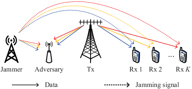
We assume that the transmitter has $M$ ($M\geq 1$) antennas and that the $K$ receivers, the adversary, and the jammer each have a single antenna. For convenience, assume that the transmitter uses the $k$-th orthogonal frequency band to communicate with the $k$-th receiver where $1\leq k\leq K$. We consider a block fading channel model. Specifically, the channel coefficients remain unchanged in each channel coherent time block and are identically and independently distributed (i.i.d.) in different time blocks. Besides, the channel coefficients in different frequency bands are also i.i.d. For simplicity, we assume that all the channels share the same channel coherent time. In the $i$-th ($i\geq 1$) time block, denote by $\bm{h}_{k,i}\sim\mathcal{CN}(\bm{0},\bm{I}_{M})$ and $\phi_{k,i}\sim\mathcal{CN}(0,1)$ the small-scale fading channels from the $k$-th receiver to the transmitter and the jammer, respectively. Denote by $\bm{g}_{k,i}\sim\mathcal{CN}(\bm{0},\bm{I}_{M})$ and $\varphi_{k,i}\sim\mathcal{CN}(0,1)$ the small-scale fading channels from the transmitter and the jammer to the adversary in the $k$-th frequency band, respectively.

We consider that the communication system works in time division duplex mode. In each channel coherent time block, which consists of $N$ ($N>1$) symbol periods, each receiver first sends a pilot sequence of length $N_{t}$ to the transmitter, and the transmitter estimates the channels by exploiting the channel reciprocity. After that, the transmitter uses the remaining $N_{d}=N-N_{t}$ symbol periods to transmit its data to the receivers. In the $i$-th time block, the pilot sequence received by the transmitter in the $k$-th frequency band is

where $P_{{\rm R}_{k}}$ is the transmit power of the $k$-th receiver, $S_{{\rm R}_{k},{\rm T}}$ is the distance-based path loss between the $k$-th receiver and the transmitter, $\bm{x}_{k}^{(p)}\in\mathcal{C}^{N_{t}\times 1}$ is the pilot sequence sent by the $k$-th receiver, and $\bm{Z}_{k,i}\in\mathcal{C}^{M\times N_{t}}$ is the AWGN with each of its elements distributed as $\mathcal{CN}(0,\sigma_{k,\rm{T}}^{2})$. For notation simplicity, we assume that $P_{{\rm R}_{1}}=\cdots=P_{{\rm R}_{K}}=P_{\rm R}$ and $\sigma_{1,\rm{T}}^{2}=\cdots=\sigma_{K,\rm{T}}^{2}=\sigma_{\rm{T}}^{2}$. Based on (1), the minimum mean square error estimation of $\bm{h}_{k,i}$, denoted by $\hat{\bm{h}}_{k,i}$, and the estimation error, denoted by $\tilde{\bm{h}}_{k,i}$, are respectively given by

where $\mu_{k}\triangleq\frac{\sigma_{\rm{T}}^{2}}{P_{\rm R}S_{{\rm R}_{k},{\rm T}}}$. After obtaining $\hat{\bm{h}}_{k,i}$, the transmitter adopts the maximum ratio transmission beamforming scheme to transmits its data to the $k$-th receiver, and the beamforming vector is given by $\bm{b}_{k,i}=\frac{\hat{\bm{h}}_{k,i}}{||\hat{\bm{h}}_{k,i}||}$. Accordingly, the $k$-th receiver receives

where $P_{k}$ is the transmit power allocated for the $k$-th receiver, $\bm{x}_{k,i}^{(d)}\sim\mathcal{CN}(0,\bm{I}_{N_{d}})$ is the data sequence, $Q_{k}$ is the jamming power that the jammer emits in the $k$-th frequency band, $S_{{\rm R}_{k},\rm J}$ is the path loss between the $k$-th receiver and the jammer, $\bm{v}_{k,i}\sim\mathcal{CN}(0,\bm{I}_{N_{d}})$ is a sequence of the jamming signals transmitted by the jammer, and $\bm{z}_{k,i}\sim\mathcal{CN}(0,\sigma_{{\rm R}_{k}}^{2}\bm{I}_{N_{d}})$ is the AWGN. It is worth noting that by (1) and (4), we assume that the jammer keeps silent during the channel training process and jams the $K$ frequency bands during the data transmission process.

From the perspective of the adversary, it does not know whether communication occurs or not, and the signals received by the adversary in the $i$-th time block can be modeled as

where $k\in\{1,2,\cdots,K\}$, $\mathcal{H}_{1}$ and $\mathcal{H}_{0}$ stand for the hypotheses that communication occurs and does not occur, respectively, $\bm{w}_{k}(i)\in\mathcal{C}^{N_{d}\times 1}$ is the signal received in the $k$-th frequency band, $S_{{\rm A},{\rm T}}$ and $S_{\rm A,J}$ are the path losses from the transmitter and the jammer to the adversary, respectively, and $\tilde{\bm{z}}_{k,i}\sim\mathcal{CN}\left(\bm{0},\sigma_{{\rm A}_{k}}^{2}\bm{I}_{M}\right)$ is the AWGN. We assume that the adversary does not know the instantaneous channel realizations, i.e., $\varphi_{k,i}$ and $\bm{g}_{k,i}$ for $1\leq k\leq K$, but knows their statistic distributions. Besides, we assume that the jamming powers, i.e., $Q_{k}$ for $1\leq k\leq K$, are fixed constants.

The goal of the adversary is to determine whether or not communication occurs based on its received signals in the $K$ frequency bands. We consider the following two scenarios depending on the temporal dynamic properties of the wireless channels:

By assumption, the adversary independently runs its detection process in each single time block. In the $i$-th time block, the detection problem at the adversary can be formulated as the following binary hypothesis testing problem,

where $\bm{w}_{k}(i)$, $1\leq k\leq K$, are defined in (5), $f_{1}^{(N_{d})}$ and $f_{0}^{(N_{d})}$ are the PDFs of $\bm{W}(i)$ under the condition that transmission occurs and does not occur in the $i$-th time block, respectively. For notation simplicity, we omit the time block index $i$ in the subsequent part of this section.

Define $U_{k}\triangleq P_{k}S_{{\rm A},{\rm T}}|\bm{g}_{k}^{H}\bm{b}_{k}|^{2}+Q_{k}S_{{\rm A},{\rm J}}|\varphi_{k}|^{2}+\sigma_{{\rm A}_{k}}^{2}$ and $V_{k}\triangleq Q_{k}S_{{\rm A},{\rm J}}|\varphi_{k}|^{2}+\sigma_{{\rm A}_{k}}^{2}$, and then $f_{1}^{(N_{d})}$ and $f_{0}^{(N_{d})}$ can be written as

where $f_{1,k}^{(N_{d})}(\cdot)\triangleq\mathbb{E}_{U_{k}}\left\{f^{(N_{d})}(\cdot|U_{k})\right\}$, $f_{0,k}^{(N_{d})}(\cdot)\triangleq\mathbb{E}_{V_{k}}\left\{f^{(N_{d})}(\cdot|V_{k})\right\}$, and for $x>0$, $f^{(N_{d})}(\bm{w}_{k}|x)\triangleq\frac{1}{\pi^{N_{d}}x^{N_{d}}}\mathrm{e}^{-\frac{\bm{w}_{k}^{H}\bm{w}_{k}}{x}}$ is the PDF of a circular symmetrical complex Gaussian random vector with covariance matrix $x\bm{I}_{N_{d}}$. The PDFs of $U_{k}$ and $V_{k}$ are presented in the following lemma.

In previous subsection, we have presented our method to reformulate the covertness constraint. In this subsection, we maximize the effective sum-rate subject to the covertness constraint (20).

For the case with $K=1$, based on (17), we ensure the covertness of the communication by letting $\chi_{1}^{\frac{1}{1-\chi_{1}}}\leq\epsilon$. As a result, the maximal feasible transmit power is given by $P_{1}^{*}=\frac{\chi^{*}\hat{q}_{1}}{S_{\rm A,T}}$, where $\chi^{*}$ is the unique solution to $x^{\frac{1}{1-x}}=\epsilon$ in $(0,1)$. Substituting $P_{1}^{*}$ into (9), we obtain the following problem,

where $\gamma_{1}\triangleq\mathrm{e}^{r_{1}}-1$ is viewed as the optimization variable, $A_{1}\triangleq\frac{S_{{\rm R}_{k},{\rm T}}S_{\rm A,J}}{S_{{\rm R}_{k},\rm J}S_{\rm A,T}}||\bm{h}_{1}||^{2}$ and $B_{1}\triangleq\mathrm{e}^{\sigma_{{\rm R}_{k}}^{2}/(Q_{1}S_{{\rm R}_{k},\rm J})}$. The optimal solution to (21), denoted by $\gamma_{1}^{*}$, is presented below.

References

- [1] X. You et al.., “Towards 6G wireless communication networks: vision, enabling technologies, and new paradigm shifts,” Sci. China Inf. Sci., vol. 64, no. 1, Jan. 2021, doi: 10.1007/s11432-020-2955-6.
- [2] B. Ai, A. F. Molisch, M. Rupp and Z. -D. Zhong, “5G Key Technologies for Smart Railways,” in Proceedings of the IEEE, vol. 108, no. 6, pp. 856–893, Jun. 2020
- [3] B. A. Bash, D. Goeckel, D. Towsley, and S. Guha, “Hiding information in noise: Fundamental limits of covert wireless communication,” IEEE Commun. Mag., vol. 53, no. 12, pp. 26–31, Dec. 2015.
- [4] S. Yan, X. Zhou, J. Hu, and S. V. Hanly, “Low probability of detection communication: Opportunities and challenges,” IEEE Wireless Commun., vol. 26, no. 5, pp. 19–25, Oct. 2019.
- [5] B. A. Bash, D. Goeckel, and D. Towsley, “Limits of reliable communication with low probability of detection on AWGN channels,” IEEE J. Sel. Areas Commun., vol. 31, no. 9, pp. 1921–1930, Sep. 2013.
- [6] P. H. Che, M. Bakshi, and S. Jaggi, “Reliable deniable communication: Hiding messages in noise,” 2013 IEEE International Symposium on Information Theory, Istanbul, 2013, pp. 2945–2949.
- [7] M. R. Bloch, “Covert communication over noisy channels: A resolvability perspective,” IEEE Trans. Inf. Theory, vol. 62, no. 5, pp. 2334–2354, May 2016.
- [8] L. Wang, G. W. Wornell, and L. Zheng, “Fundamental limits of communication with low probability of detection,” IEEE Trans. Inf. Theory, vol. 62, no. 6, pp. 3493–3503, Jun. 2016.
- [9] S. Lee, R. J. Baxley, M. A. Weitnauer, and B. Walkenhorst, “Achieving undetectable communication,” IEEE J. Sel. Topics Signal Process., vol. 9, no. 7, pp. 1195–1205, Oct. 2015.
- [10] D. Goeckel, B. Bash, S. Guha and D. Towsley, “Covert communications when the warden does not know the background noise power,” IEEE Commun. Let., vol. 20, no. 2, pp. 236-239, Feb. 2016.
- [11] B. A. Bash, D. Goeckel, and D. Towsley, “Covert communication gains from adversary’s ignorance of transmission time,” IEEE Trans. Wireless Commun., vol. 15, no. 12, pp. 8394–8405, Dec. 2016.
- [12] K. S. K. Arumugam and M. R. Bloch, “Keyless asynchronous covert communication,” in Proc. 2016 IEEE Information Theory Workshop (ITW), Cambridge, 2016, pp. 191–195.
- [13] K.-W Huang, H.-M Wang, D. Towsley, and H. V. Poor, “LPD communication: A sequential change-point detection perspective,” IEEE Trans. Commun., vol. 68, no. 4, pp. 2474–2490, April 2020.
- [14] B. He, S. Yan, X. Zhou, and H. Jafarkhani, “Covert wireless communication with a poisson field of interferers,” IEEE Trans. Wireless Commun., vol. 17, no. 9, pp. 6005–6017, Sep. 2018.
- [15] T.-X. Zheng, H.-M. Wang, D. W. K. Ng and J. Yuan, “Multi-antenna covert communications in random wireless networks,” IEEE Trans. Wireless Commun., vol. 18, no. 3, pp. 1974–1987, Mar. 2019.
- [16] Y. Jiang, L. Wang, and H. Chen, “Covert communications in D2D underlaying cellular networks with antenna array assisted artificial noise transmission,” IEEE Trans. Veh. Tech., 2020.
- [17] J. Hu, S. Yan, F. Shu, and J. Wang, “Covert transmission with a self-sustained relay,” IEEE Trans. Wireless Commun., vol. 18, no. 8, pp. 4089–4102, Aug. 2019.
- [18] J. Hu, S. Yan, X. Zhou, F. Shu, J. Li and J. Wang, “Covert communication achieved by a greedy relay in wireless networks,“ IEEE Trans. Wireless Commun., vol. 17, no. 7, pp. 4766–4779, Jul. 2018.
- [19] D. Goeckel, A. Sheikholeslami, T. Sobers, B. A. Bash, O. Towsley, and S. Guha, “Covert communications in a dynamic interference environment,” 2018 IEEE 19th International Workshop on Signal Processing Advances in Wireless Communications (SPAWC), Kalamata, 2018, pp. 1–5.
- [20] T. V. Sobers, B. A. Bash, S. Guha, D. Towsley, and D. Goeckel, “Covert communication in the presence of an uninformed jammer,” IEEE Trans. Wireless Commun., vol. 16, no. 9, pp. 6193–6206, Sep. 2017.
- [21] K. Li, P. A. Kelly and D. Goeckel, “Optimal power adaptation in covert communication with an uninformed jammer,” IEEE Trans. Wireless Commun., vol. 19, no. 5, pp. 3463–3473, May 2020.
- [22] R. Soltani, D. Goeckel, D. Towsley, B. A. Bash and S. Guha, “Covert wireless communication with artificial noise generation,” IEEE Trans. Wireless Commun., vol. 17, no. 11, pp. 7252–7267, Nov. 2018.
- [23] M. Forouzesh, P. Azmi, N. Mokari and D. Goeckel, “Covert communication using null space and 3D beamforming: Uncertainty of Willie’s location information,” IEEE Trans. Veh. Techn., 2020.
- [24] O. Shmuel, A. Cohen, O. Gurewitz and A. Cohen, “Multi-antenna jamming in covert communication,” 2019 IEEE International Symposium on Information Theory (ISIT), Paris, France, 2019, pp. 987-991.
- [25] K. Shahzad, X. Zhou, S. Yan, J. Hu, F. Shu, and J. Li, “Achieving covert wireless communications using a full-duplex receiver,” IEEE Trans. Wireless Commun., vol. 17, no. 12, pp. 8517-8530, Dec. 2018.
- [26] F. Shu, T. Xu, J. Hu, and S. Yan, “Delay-constrained covert communications with a full-duplex receiver,” IEEE Wireless Commun. Let., vol. 8, no. 3, pp. 813-816, June 2019.
- [27] J. Hu, S. Yan, X. Zhou, F. Shu, and J. Li, “Covert wireless communications with channel inversion power control in rayleigh fading,” IEEE Trans. Veh. Tech., vol. 68, no. 12, pp. 12135–12149, Dec. 2019.
- [28] J. Jose, A. Ashikhmin, T. L. Marzetta, and S. Vishwanath, “Pilot contamination and precoding in multi–cell TDD systems,” IEEE Trans. Wireless Commun., vol. 10, no. 8, pp. 2640–2651, Aug. 2011.
- [29] I. S. Gradshteyn, I. M. Ryzhik, A. Jeffrey, D. Zwillinger, and S. Technica, Table of integrals, series, and products, 7th ed. New York, NY, USA: Academic, 2007.
- [30] H. Tuy, F. A. khayya and P. Thach, “Monotonic optimization: Branch and cut methods” in Essays and Surveys in Global Optimization, New York, NY, USA:Springer, pp. 39–78, 2005.
- [31] Y. J. Zhang, L. Qian, and J. Huang, “Monotonic optimization in communication and networking systems,” Now Publishers: Foundations and Trends in Networking, vol. 7, no. 1, 2012.
- [32] A. Beck, A. B. Tal, and L. Tetruashvili, “A sequential parametric convex approximation method with applications to nonconvex truss topology design problems”, J. Global Opt., vol. 47, no. 1, pp. 29–51, 2010.
- [33] M. Razaviyayn, “Successive convex approximation: Analysis and applications,” Ph.D. dissertation, Univ. Minnesota, Minneapolis, MN, USA, 2014.
- [34] E. Lehmann and J. Romano, Testing Statistical Hypotheses, 3rd ed. New York: Springer, 2005.
- [35] E. Stein and R. Shakarchi, Real Analysis: Measure Theory Integration and Hilbert Spaces, NJ, Princeton:Princeton Univ. Press, 2005.
- [36] T. M. Cover and J. A. Thomas, Elements of Information Theory, 2nd ed. John Wiley & Sons, Hoboken, NJ, 2002.
- [37] S. Boyd and L. Vandenberghe, Convex Optimization, Cambridge, U.K.: Cambridge Univ. Press, 2004.
- [38] M. Grant and S. Boyd, CVX: MATLAB Software for Disciplined Convex Programming, [Online]. Available: http://cvxr.com/cvx.