The OPE meets semiclassics
Abstract
We show that the correlator of three large charge operators with minimal scaling dimension can be computed semiclassically in CFTs with a symmetry for arbitrary fixed values of the ratios of their charges. We obtain explicitly the OPE coefficient from the numerical solution of a nonlinear boundary value problem in the conformal superfluid EFT in . The result applies in all three-dimensional CFTs with a symmetry whose large charge sector is a superfluid.
I Introduction
The emergence of classical physics at large quantum numbers is a concept familiar since the early developments of quantum-mechanics landau1958quantum. Well-known examples include the rigid rotor and the hydrogen atom. In both these cases, the path integral computing the wave function of states with large angular momentum is dominated by a classical saddle-point trajectory. The expansion around this classical configuration coincides with an expansion in inverse powers of (see e.g. MoninCFT for an illustration). A similar picture underlies certain simplifications in the study quantum field theories, such as the BMN limit in super-Yang-Mills theory Berenstein:2002jq, the large spin limit of double-trace operators in conformal theories (CFTs) Alday:2007mf; Komargodski:2012ek; Fitzpatrick:2012yx or the effective description of large spin mesons as semiclassical rotating strings Hellerman:2013kba. Recently, the connection between semiclassics and large quantum number has also provided a useful inspiration in the study of operators carrying a large conserved internal charge in conformal field theories.
The interest toward this problem stems from the remarkable fact that the large charge sector of many, otherwise nearly intractable, strongly coupled CFTs has been argued to admit a universal weakly coupled description in terms of a certain number of hydrodynamic Goldstone modes Hellerman. This is because, by the state-operator correspondence, large charge operators are associated with states with large charge density for the theory quantized on the cylinder. Analogously to the aforementioned quantum-mechanical examples, one then expects the path integral describing their time evolution to be dominated by a classical trajectory. This in turn will generically break the internal group as well as certain spacetime symmetries MoninCFT. Taking the internal group to be for concreteness, the simplest possibility for the symmetry-breaking pattern is the one defining a superfluid phase, which admits a simple effective field theory (EFT) description in terms of a single Goldstone mode Son:2002zn. In the EFT, the systematic derivative expansion coincides with an expansion in inverse powers of the charge; this makes it possible to study perturbatively the spectrum of charged operators of the theory. Extensions of this idea have also been applied in related problems in CFTs, such as the study of -charged operators in superconformal theories Hellerman:2017veg; Hellerman:2017sur or the determination of the spectrum of spinning charged operators Cuomo:2017vzg.
The cylinder viewpoint is illuminating in the study of the spectrum of charged operators. However, it does not seem to provide a useful starting point in the study of correlators with more than two large charge operator insertions,11 1 It is trivial to extend the analyses of Hellerman; Badel to compute correlation functions of light operators in between two large charge operators; see e.g. MoninCFT; Jafferis:2017zna or the discussion below Eq. (46). that so far eluded our understanding (in the non-supersymmetric case22 2 For theories with extended supersymmetry a lot of progress has been achieved in the study of protected operators, see e.g. Grassi:2019txd; Bargheer:2019kxb; Bargheer:2019exp; Hellerman:2020sqj in a similar context. ). In fact, from that perspective it is not even clear if correlators of large charge operators should be calculable within EFT. This is because known EFT descriptions of CFT operators are often associated with the existence of an appropriate macroscopic limit Lashkari:2016vgj; Jafferis:2017zna, in which the radius of the sphere is sent to infinity while the local charge and energy densities are kept finite. This limit is most naturally formulated for correlators involving two heavy operators, hence with large scaling dimension, and possibly additional insertions of light operators, whose scaling dimension is much smaller than the heavy ones and whose insertion can be thought as a small perturbation of the heavy states.
However, as we will argue in this paper, the EFT in fact allows also for the controlled calculation of three- and higher-point function of large charge operators. Physically this is because, in radial quantization, each operator creates a superfluid state with charge around the insertion point . The three-point function then describes the transition between the different superfluids, which is associated with a new classical trajectory in the path integral. Since the radial fields are locally gapped around each state, the corresponding modes are not excited by the classical profile, that thus can be reliably computed within EFT.
Let us call the operator with minimal scaling dimension with charge and its hermitian conjugate. Focusing on three-dimensional CFTs, we will show that the calculation of the three-point function , to leading order in the charge and for arbitrary values of the ratio , reduces to the solution of a boundary value problem. Solving this problem numerically, we obtain the operator product expansion (OPE) coefficient. The result takes the form
| (1) |
Here is the unique Wilson coefficient upon which the EFT depends at leading order and the function is plotted in Fig. 2. We expect that the result Eq. (1) applies in several theories. For instance, we expect that Eq. (1) describes the OPE coefficient of the three operators with minimal scaling dimension at fixed large values of their charges in the model, where Monte Carlo simulations found Banerjee:2017fcx. To the best of our knowledge, Eq. (1) represents the only example of a universal correlator of three heavy operators in CFT which has been computed (so far) without supersymmetry in .33 3 For related results in see Gross:1987ar and more recently Cardy:2017qhl; Collier:2019weq; Belin:2020hea.
While the main focus of this paper is on the general superfluid EFT, our ideas might also be of some relevance in the study of weakly coupled theories. It has been recently shown that a semiclassical approach can be used to overcome the breakdown of perturbation theory in the determination of the scaling dimensions of large charge operators in the epsilon expansion Badel. In Appendix A we discuss the semiclassical problem associated with the calculation of the three-point function in the tricritical model in dimension. There we show that our formulation allows to overcome some technical issues with the generalization of the approach of Badel to higher-point functions. The formulation of the problem will make manifest that the calculation reduces to the one in the EFT discussed in the main text in the appropriate regime. A numerical solution can be obtained in more general regimes as well, but we leave a detailed investigation for future work.
The rest of the paper is organized as follows. In Sec. II we briefly review the structure of the EFT and explain how to use it to compute flat space correlators in the large charge regime. In Sec. III we discuss the three-point function. We formulate and solve the associated boundary value problem in Sec. III.1. The result is discussed in Sec. III.2. We comment on future directions in Sec. IV. The Appendix contains a formal discussion of three-point functions of large charge operators in the weakly coupled tricritical model in dimensions.
II Flat space correlators from EFT
We expect that correlators of large charge operators in three-dimensional CFTs admit a universal EFT description in terms of a single Goldstone boson Hellerman; MoninCFT:
| (2) |
Previous works generically considered the action (2) on , which provides a natural starting point to study the spectrum of the theory. However, the Weyl invariance of the action ensures that the same results can be recovered working directly in flat space. As a warmup to the study of the three-point function, here we illustrate this point explicitly for the calculation of the two-point function of the charge operator with minimal scaling dimension.
In order to proceed, we should find a suitable definition of the operator. To this aim, we notice that, by the state-operator correspondence, an insertion of the operator at the point in a generic correlator may be equivalently represented by cutting the path integral around a ball of radius , and specifying appropriate boundary conditions for the fields on the surface Simmons-Duffin:2016gjk. These follow from performing the path integral inside the ball. For the path integral inside is independent of the other operator insertions; hence in this limit we can use the boundary conditions on to fully specify the operator. Notice that the infinitesimal radius of the ball provides a natural regulator for the divergences associated with the wave function renormalization of the operator.
In principle, the appropriate definition of the state on , and hence of the corresponding operator, can always be found solving the functional Schrödinger equation in radial quantization. In practice, for the operator it is easier to just guess the result. Here we just provide the prescription. We will see later that this indeed reproduces the expected form of the two-point function, hence proving that our guess is correct.
To specify an insertion of the operator with minimal scaling dimension with charge at the point , we add to the action a boundary term of the form MoninCFT
| (3) |
where is the volume element on . The boundary term (3) may be thought as a wave functional for the state in radial quantization and fixes its charge to be . Notice that imposing that the variation of the action (2) plus the boundary term (3) vanishes implies that, on the saddle-point solution, the Noether current approaches the form expected from spherical symmetry and Gauss’s law close to the insertion point:
| (4) |
In general, to compute -point functions of the operator , we cut the path integral around different points with balls of infinitesimal radius , and we add a boundary term of the form (3) for each insertion.
We are now ready to compute the two-point function. The leading-order result is given by:
| (5) |
where the action and the boundary terms are calculated on the profile which solves the saddle-point equation:
| (6) |
with boundary conditions (4) for (with the replacement for ). The solution reads:
| (7) |
The physical meaning of this solution is simply understood. Set to be the origin of space and take the limit . Then Eq. (7) reads:
| (8) |
which, unsurprisingly, is nothing but the superfluid profile considered in Hellerman. The conformal equivalence with the solution (8) and the Weyl invariance of the theory ensure that higher derivative corrections are always suppressed with respect to the leading order for .
We may now use the solution (7) to compute the classical action (5). We find:
| (9) |
where and
| (10) |
This agrees with the result for the scaling dimension first obtained in Hellerman. The value of the normalization is unphysical, but it will be important to properly (re)normalize the three-point function and extract the OPE coefficient.
Notice that the form of the solution (7) is totally fixed by conformal invariance. This is because the classical expectation value for the current physically represents a (normalized) correlator of three primary operators:
| (11) |
which is equivalent to Eq. (7) after using the result for the correlator on the right-hand side based on the Ward identities and conformal invariance. This provides an alternative proof that Eq. (3) indeed defines a scalar primary operator.
Finally we remark that a definition analogous to Eq. (3) can be used to simplify the study of flat space correlators of large charge operators directly in the UV theory, when the latter is weakly coupled. In that case, the definition of the operator should be supplemented by appropriate boundary conditions for the radial components of the fields of the model on the surface of the ball. We show an example in Sec. A.3 of the Appendix for the tricritical fixed point in dimensions.
III The three-point function
In the previous section we explained how to compute flat space correlators and we exemplified our approach with the calculation of the two-point function. In this section we formulate and solve the semiclassical problem associated with the three-point function. Though we were only able to obtain a numerical result, we provide approximate analytic expressions in different limits.
Physically, the reason why we can compute -point functions within the EFT is that all the operator insertions specify a superfluid state with large chemical potential . Local excitations of the radial mode are separated by a large gap with respect to the Goldstone modes close to these points. Hence, if the transition between the different superfluid states is sufficiently smooth, these will not be excited by the solution - which can then be computed within EFT. More technically, the calculation of the saddle-point requires control over the full nonlinear structure of the leading-order action (2), but it only receives small corrections from the higher derivative terms.44 4 This is analogous to what happens in gravity, where many interesting solutions follow from the nonlinear structure of the Einstein-Hilbert action, but they are largely unaffected by higher curvature corrections.
III.1 Numerical solution
The general form of the three-point function is:
| (12) |
where is the OPE coefficient and we defined
| (13) |
with , and . Notice that since we can always redefine , with , the phase of the OPE coefficient is unphysical. For concreteness we consider .
According to the prescription explained in Sec. II, to compute the three-point function we need to solve the problem specified by the action:
| (14) |
where
| (15) |
with , and . This is equivalent to solving the equation of motion (6) with boundary conditions in the form (4) close to the insertion points.
To write a convenient ansatz for the solution, we notice that the solution depends on four points ( and the insertion points). Conformal invariance then suggests to introduce cross-ratios as
| (16) | ||||
| (17) |
where . The solution may then be parametrized as:
| (18) |
where is purely real and and are defined in Eq. (16). Formally, this ansatz can be justified by arguments similar to that explained above Eq. (11). The physical meaning of the coordinates (16) is understood noticing that the bulk equation of motion (6) is equivalent to current conservation for the theory on in terms of and .
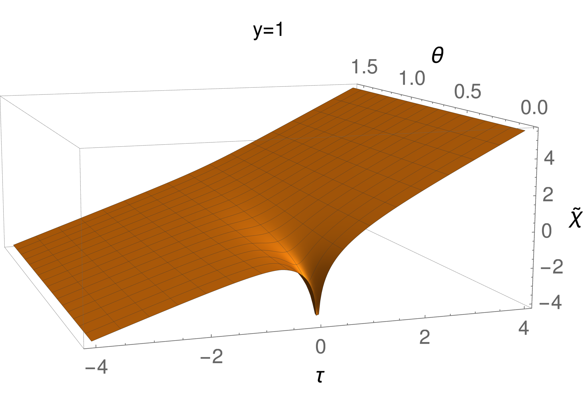
Working with the rescaled field in Eq. (18) is convenient since its value depends on the ratio , but not on . Indeed, the bulk Eq. (6) is independent of any field rescaling, while the boundary conditions for depend only on . Explicitly, the expansion of the field at the boundary points read:
| (19) | ||||
Eq. (19) shows that, in this parametrization, the saddle-point profile takes a superfluid form at . The singularity at provides the source which accounts for the mismatch in the charge fluxes at and . In Eq. (19), besides showing the leading behavior to be imposed in the solution, we also defined the first constant corrections to the field close to the insertion points, whose value is determined solving the equations of motion. Finally we stressed that the additional corrections to the boundary values at decay exponentially fast.55 5 The form of the solution close to the insertion points is obtained linearizing the equation around the profile dictated by the boundary conditions.
Discretizing the equation as explained in Krikun:2018ufr and introducing a sufficiently large cutoff for , it is now possible to solve for the profile numerically. The typical shape of the solution is shown in Fig. 1. As it may be seen from there, is regular everywhere but at the insertion points, where the solution however is conformally equivalent to a superfluid profile. Hence higher derivative corrections to the EFT (2) are always suppressed by with respect to the leading term, provided . This justifies the use of the action (2) a posteriori.
We now use the numerical solution for the profile to extract the OPE coefficient. To this aim we notice that the action (14) on shell reduces to a boundary term. Therefore, we find that the OPE coefficient may be written purely in terms of the boundary coefficients defined in eq. (19):
| (20) |
where . From the behavior of the numerical solution close to the insertion points we determine the ’s and we use them to compute the function . The numerical result is plotted in Fig. 2 for . This range fully determines the OPE coefficient, since by permutation symmetry we must have . We verified that this relation is satisfied within the numerical error for . 66 6 The result plotted in 2 was obtained discretizing the equation on a grid with , uniformly discretized in points. Different choices of the grid provided compatible results within the numerical uncertainty. A fourth-order approximation was used to discretize the derivatives. We also made use of the shift symmetry of to set in Eq. (19). From the variance around the mean value of the field at , we estimated the numerical error on , from which we found the relative uncertainty on to be for all values of .
III.2 Analysis of the result
Eq. (20) with the numerical result plotted in Fig. 2 is the main result of this paper. Here we discus its behaviour for small and for .
In the regime we may compare the result with the EFT prediction for the OPE coefficient of a light operator in between two large charge ones. This is given by MoninCFT; Cuomo:2020rgt:
| (21) |
where is a Wilson coefficient, which may depend on but not on . Such form is compatible with our result (20) for provided the coefficient takes the form:
| (22) |
where is a constant which does not depend on the charge. This implies that the function in Eq. (20) admits the following expansion for small :
| (23) |
This is in good agreement with our numerical result. More precisely, retaining only the leading order we find agreement up to relative for . The comparison of Eq. (23) with our numerical result for can be used to determine . Even including the subleading terms, for , which is equivalent to , the prediction (23) and the numerical results start to differ significantly. In particular, the expansion (23) obviously cannot be extrapolated to . The comparison is summarized in Fig. 3.
For the result (20) can be seen as a resummation of infinite perturbative corrections to the OPE coefficient computed in MoninCFT; Cuomo:2020rgt for . We find and in general for . Hence Eq. (20) predicts that the fusion coefficient for three operators of charge grows faster than exponentially, as . As for the scaling dimension (10), the power just follows from dimensional analysis and semiclassics. In fact the value of the Lagrangian, locally, is naturally set by the largest dimensionful scale for the theory on , which is given by the charge density . Dimensional analysis implies , from which the scaling follows. Notice also that the non-polynomial growth in Eq. (20) is not compatible with a finite macroscopic limit as defined in Jafferis:2017zna.
Eq. (20) is reminiscent of the result of Cardy:2017qhl; Collier:2019weq, where it was shown that the average value of the OPE coefficient for three heavy operators obtained in CFTs grows as , where is an number. As commented in Cardy:2017qhl, this growth is not surprising. Indeed Eq. (20) describes a correlation function with operators located at , and , but this is only a convention. A different choice of the operator positions would change the correlation function by an exponential factor, and could possibly cancel the growth of the result (20).
We may also use permutation symmetry to provide an approximate expression for when . Indeed Taylor expanding the relation we conclude , from which we infer:77 7 In general, the functional equation relates and a linear combination of even derivatives of lower order, . For instance, the value of can be used to improve the approximation (24) with two more terms. Comparing different numerical fits we found a relatively small value for the second derivative , justifying the accuracy of the linear interpolation (24).
| (24) |
Eq. (24) agrees with our numerical result up to relative for .
We summarize the comparison between the approximations that we discussed and the numerical result in Fig. 4. We see that, though we have not been able to compute the OPE coefficient (20) in a closed analytic form, the approximate expressions (23) and (24) combined suffice to give a numerically accurate description of the result up to relative for all values of .
IV Outlook
In this paper we illustrated how to compute semiclassically three-point functions of large charge operator in three-dimensional invariant CFTs. Our main result, Eq. (20), provides a novel general prediction for the OPE coefficient of three large charge operators with minimal scaling dimensions. This prediction applies in all CFTs whose large charge sector is in a superfluid phase. For instance, we expect that it applies in the model, where in principle it may be tested via Monte Carlo simulations, along the lines of Banerjee:2017fcx.
Our work admits some obvious extensions. As already mentioned, it is possible to obtain numerical results for the OPE coefficients directly in weakly coupled models, such as the tricritical model in dimensions discussed in Appendix A, or, via an obvious generalization, in the Wilson-Fisher fixed-point in dimensions. Perhaps, a similar procedure might be applied in the models at large as well (see Alvarez-Gaume:2019biu; Giombi:2020enj for recent progress in the study of large charge operators at large ). It is also possible to study higher-point functions. For instance, generalizing Eq. (18), we expect that the semiclassical solution determining the correlator of four charged operators will depend on five independent cross ratios. Three of them will be given by the independent components of the coordinate , while the other two should coincide with the two physical cross-ratios specifying the configuration in the four-point function. A detailed analysis of this problem within the large charge EFT would allow for the determination of OPE coefficients involving operators corresponding to phonon excitations on top of the superfluid ground state Hellerman. It would also be interesting, but probably technically challenging, to extend our analysis to subleading order in derivatives and to include quantum effects. Notice however that in the EFT quantum corrections to the OPE coefficient scale only as , and are hence quite suppressed with respect to the leading order.
To the best of our knowledge, the result (20) represents the only example of a universal correlator of three heavy operators in CFT which has been computed without supersymmetry in . The universal nature of the result stems from the fact that it has been obtained within the conformal superfluid EFT. Differently from matrix elements of the form heavy-light-heavy, which are obtained considering small perturbations of the heavy state MoninCFT, the result was obtained considering a new saddle point profile, which accounts for the classical nonlinearities of the action exactly. Perhaps a similar approach might extend the existing result on heavy-light-heavy OPE coefficients of generic (not necessarily charged) operators, which are based on thermodynamics and hydrodynamics Lashkari:2016vgj; Delacretaz:2020nit, to the heavy-heavy-heavy regime.
In the case of weakly coupled theories, the semiclassical approach can be used to overcome the breakdown of perturbation theory for multi-legged amplitudes describing large charge operators Badel. For instance, in the tricritical model in dimensions discussed in the Appendix A, the result (20) can be seen as a resummation of infinite Feynman diagrams in the regime , where is the perturbative coupling. The connection between semiclassics and multi-legged amplitudes was first appreciated in the study of multiparticle production processes Rubakov:1995hq, where the physical rate was shown to be associated with the solution of a semiclassical boundary value problem Son:1995wz. Unfortunately, the status on the solution of the latter is still a controversial subject to this date (see e.g. Khoze:2018mey and Monin:2018cbi for the two opposite viewpoints). It is interesting to compare that semiclassical problem with the one considered in this work. Somewhat similarly to the situation considered in Sec. III.1, where the singularity of the solution in Fig. 1 ensures that Gauss’s law holds globally, the solution to the problem of Son:1995wz requires a singular field configuration to account for the change in the energy (the production by a source) between the initial and the final state. However, differently from the case of CFT correlators, the multiparticle production classical problem does not admit a fully Euclidean formulation. Perhaps more importantly, at present there is no clear EFT picture for the corresponding physical process. This is again different from the problem that one encounters in the study of large charge CFT operators in perturbative theories, addressed for the first time in Badel, whose solution was indeed almost completely guided by previous EFT developments in the same context Hellerman; MoninCFT.
Acknowledgements
I thank Zohar Komargodski, Alexander Monin, Sridip Pal and Riccardo Rattazzi for inspiring discussions, and I am especially grateful to João Penedones for collaboration at the early stages of this work. It is also a pleasure to thank my father, Massimo Cuomo, for delightful discussions on numerical methods. My work is supported by the Simons Foundation (Simons Collaboration on the Non-perturbative Bootstrap) grants 488647 and 397411.
Appendix A The three-point function boundary value problem in a weakly coupled model
In this Appendix we generalize the approach in the main text to the calculation of three-point functions of large charge operators in weakly coupled theories, focusing on the tricritical fixed point in dimensions for illustration.
It has been shown in Badel; Badel2 that the scaling dimension of the operator can be computed semiclassically as an expansion in the coupling at arbitrary fixed values of , which plays a role analogous to the ‘t Hooft coupling in large N gauge theories. The same approach has been successfully applied in the calculation of two-point function of charged operators in several different models (see e.g. Antipin:2020abu; Giombi:2020enj), but technical difficulties make the generalization of the method to higher-point functions non-straightforward. Here we show that the calculation of the three-point function in the perturbative model can be reduced, to leading order in but to all orders in and , to the solution of a boundary value problem. This problem enjoys exact conformal symmetry and, crucially, it is formulated in three Euclidean dimensions; this makes it always possible to look for a solution numerically, differently from the existing formulation of the problem based on dimensional regularization. We argue that for the solution can be found within the EFT studied in the main text. We leave for future work a detailed investigation of more general regimes.
A.1 The model
We consider the following (Euclidean) action in dimensions for a complex scalar field :
| (25) |
The beta function of the coupling starts at two-loop order, hence this model is conformal in up to . To higher orders, the theory admits an IR stable fixed point in dimensions with for Pisarski:
| (26) |
We will always work at leading order in the coupling (in the large charge double scaling limit); hence in what follows we set when not specified otherwise.
A.2 Operator insertions as boundary conditions in the double-scaling limit
We consider correlation functions of the lowest dimensional operator of charge , given by within perturbation theory. In Badel it was shown that its two-point function can be computed in the double-scaling limit , with fixed. The result takes the form
| (27) |
where , is the normalization of the operator, including its divergent wave function, and is the scaling dimension. In particular, Eq. (27) implies that the scaling dimension admits the following expansion:
| (28) |
The leading-order term arises as the result of a nontrivial saddle point which accounts for the operator insertions, and hence is purely semiclassical in nature. Formally, the saddle point equation follows from exponentiating the operator insertions and treating them as sources in the action. This leads to the following partial differential equations in :
| (29) |
For small values of we can make sense of these equations working within dimensional regularization and treating the interaction term perturbatively (see e.g. Badel; Arias-Tamargo:2019kfr). Unfortunately, it is less clear how to proceed for more general values of . To appreciate this, notice that the leading-order term in Eq. (27), while it is not affected by the renormalization of the coupling, it does contain the divergences associated with the wave function renormalization of the operator. This implies that the Eqs. (29) must be solved via analytic continuation to dimensions to regularize the result. This procedure breaks scale invariance at intermediate steps of the calculation, and it does not allow for a simple numerical formulation of the problem.88 8 The authors of Giombi:2020enj were able to solve analytically a similar saddle point problem to determine the two-point function of large traceless symmetric operators in the model at large . A similar approach might allow to solve Eqs. (29) as well, but we do not expect it to be easily generalizable to higher-point functions, in which case the saddle point solution might not be expressible in a closed analytic form.
In Badel this issue was solved exploiting the Weyl invariance of the model to map the theory to the cylinder . The state-operator correspondence then maps the operator to the lowest energy state for the theory quantized on .99 9 This is because all the other charge operators have scaling dimension larger than that of , and hence cannot mix with it within perturbation theory. Notice that this argument holds for arbitrary values of , as it follows from the result of Badel2 for the Fock spectrum of charge states on the cylinder. This allows to extract the scaling dimension from the expectation of the Euclidean evolution operator in an arbitrary state of charge , provided this has nonzero overlap with the true ground state. A clever choice of the state then allows to perform the calculation straightforwardly.
While the approach of Badel cannot be generalized to higher-point functions, we may proceed as we did for the EFT in Sec. II. Namely, we define the insertion of the operator at the point cutting the path integral around a ball , with , and specifying boundary conditions on the surface .1010 10 More precisely, this procedure specifies an operator which is equal to up to an unphysical normalization, which cancels out from observable quantities. With a slight abuse of notation, we shall call also this operator in what follows. Since the infinitesimal radius of the ball provides a natural regulator for the divergences associated with the wave function renormalization, we can work exactly in to leading order.
To choose the appropriate boundary conditions, we map to the plane the state chosen in Badel2 to perform the calculation on . To this aim it is convenient to work in polar field coordinates:
| (30) |
To specify an insertion of the operator with minimal scaling dimension with charge at the point , we add to the action a boundary term analogous to Eq. (3),
| (31) |
As in the case of the EFT, imposing that the variation of the action (25) plus the boundary term (31) vanishes implies that the Noether current takes the following form close to :
| (32) |
To fully specify the boundary value problem, and hence the operator, we need to specify another boundary condition on . It turns out that the convenient choice is to demand that takes a fixed value, given by
| (33) |
where is
| (34) |
For small one finds , while in the opposite regime . Finally, we assume that the path integral is supplemented with vanishing boundary conditions for the fields and at infinity.
In the next section we will compute the classical action obtained by expanding the path integral around the classical solution of the boundary value problem specified by two operator insertions. The result will take indeed the form of a two-point function for a primary operator with scaling dimension , hence proving that our definition indeed specifies the desired operator to leading order in the coupling. We will then use this definition to discuss the three-point function.
A.3 The two-point function in flat space
We are now ready to compute the two-point function. The leading-order result is given by:
| (35) |
where the action and the boundary terms are calculated on the profile which solves the saddle point equation:
| (36) |
with boundary conditions (32) and (33) for (with the replacement for ).
In the limit that we consider the semiclassical problem is conformally invariant. It is therefore natural to consider an ansatz in the form of a correlator of three primaries inserted at , and for the classical profile. Therefore we look for solutions of Eqs. (36) in the form:
| (37) |
where we used that has weight and mass dimension . We use a similar ansatz for :
| (38) |
where we reflected with respect to Eq. (37). Using this ansatz in the equations of motion and demanding the boundary conditions we find:
| (39) |
These equations are solved for purely imaginary as:
| (40) |
where and are given in Eqs. (33) and (34). Therefore the solution is totally specified up to rescalings of the form . Indeed, on the solution (40) the fields (37) and (38) are analytically continued away from the contour , and rescalings of the form are a symmetry of the action analytically continued to arbitrary values of the fields.
To understand the physical meaning of this solution, it is convenient to set to be the origin of space and take the limit . Then working in polar coordinates (30) for the field we recast the profile as:
| (41) |
Introducing a time coordinate and performing a Weyl map to the cylinder, Eq. (41) coincides with the superfluid profile considered in Badel2 for the theory on . Of course, this is not surprising, since our definition of the operator coincides with the prescription used to specify the charged state in Badel2.
We may now find the result for the two-point function evaluating the action on the corresponding solution. Upon integrating by parts, we find:
| (42) |
where the bulk integral is over the subtracted space . The explicit evaluation gives:
| (43) |
Overall, using Eqs. (42) and (43) in Eq. (35), we find that the two-point function takes the form (27) expected for the primary operator . The leading-order results in the double-scaling limit (27) for the operator normalization and the scaling dimension read:
| (44) |
| (45) |
The result (45) for the scaling dimension agrees with the one found in Badel2, hence proving that our prescription indeed describes the same primary operator considered there. In the small regime the expansion of may be compared to the diagrammatic result; this check was performed in Jack:2020wvs up to six-loop order, finding perfect agreement. In the regime the result reproduces the EFT result (10) with .
It is worth recalling that the technical reason why the solution to this problem reduces to the EFT for is that, in this regime, the solution (37) satisfies , while the kinetic term for the radial mode is negligible . We may therefore neglect derivatives of in the equations of motion (36), which reduce to the one deriving from (2).
While the field should always transform as a primary with half-integer scaling dimension in , the fact that the solution depends on the insertion points and as specified in Eq. (37) is a consequence of the chosen boundary conditions. This happens because the boundary conditions (32) and (33) specify a primary operator Giombi:2020enj. To appreciate this, notice that the classical expectation value for the field physically represents a (normalized) correlator of three primary operators:
| (46) |
where we stressed with the subscript class. that the left-hand side is evaluated on the saddle point solution. It is then easy to see that Eqs. (37) and (38) ensure that Eq. (46) has the right form to describe a CFT correlator of three primaries. One may similarly check that the form of the solution ensures that higher-point functions of the form are compatible with conformal invariance. Relatedly, as an obvious by-product of our analysis, we can compute an infinite number of three- and higher-point functions of light operators inserted within and .1111 11 This can also be done within the original approach of Badel.
A.4 The triple-scaling limit
As for the two-point function (27), the three-point function can be computed in the triple scaling limit , and with fixed. We assume for definiteness. The result is organized as:
| (47) |
Comparing with the general form for the three-point function (12) and taking into account the normalization of the two-point function (27), this implies that the OPE coefficient admits an expansion of the form:
| (48) |
Proceeding as commented below Eq. (46), we can compute the OPE coefficient in the regime using the classical solution (37) to extract the four-point function and matching the classical result to the OPE decomposition (see e.g. MoninCFT; Giombi:2020enj for similar calculations). The result for the fusion coefficient reads:
| (49) |
where is given by Eq. (34) with . This is equivalent to
| (50) |
Expanding for small , Eq. (49) reproduces the tree-level result (using Stirling’s formula). In the opposite regime, the result takes the form , in agreement with the EFT prediction for the OPE coefficient of a light operator of dimension and two heavy charged operators MoninCFT.
A.5 The boundary value problem
According to the prescription explained in Sec. A.2, to compute the three-point function we need to solve the problem specified by the action:
| (51) |
where
| (52) |
with , and . The boundary conditions for are specified as in Eq. (33):
| (53) |
where is given by (34) with .
To solve the equations of motion, it is natural to generalize the three-point function ansatz (37) and look for solutions which take the form of a four-point function:
| (54) |
Formally, this form of the solution follows from arguments analogous to those explained around Eq. (46).1212 12 From that perspective, the boundary conditions (32) and (33) ensure that correlation functions of light operators obey the correct OPE limits close to , and . Working in polar field coordinates (30), the ansatz (54) reads:
| (55) |
where the constant piece in is irrelevant due to the shift symmetry. The physical meaning of this parametrization is appreciated noticing that the equations of motion for and coincide with those for the theory on
| (56) |
where is the covariant derivative on . The boundary conditions set the value of the fields at and at the point :
| (57) |
The physical interpretation of the semiclassical problem is the same as in the EFT. As below Eq. (19), we defined the first corrections to the field close to the insertion points, whose value is determined solving the equations of motion.
Once the classical profile has been found, the OPE coefficient can be obtained computing the classical value of the action (14). Since the solution cannot develop singularities other than the ones required by the boundary conditions (57),1313 13 This is because, as explained below Eq. (46), the classical solution represents a physical correlator itself, whose only singularities are the ones dictated by the OPE. all the divergent contributions are absorbed by the normalization in Eq. (44) and we are left with a finite result that can be compactly written as
| (58) |
where is the following convergent integral:
| (59) |
Here is obtained subtracting the non-integrable contributions from :
| (60) |
Notice that given the boundary conditions, is purely imaginary on the saddle point, hence so are the and the OPE coefficient is real.
Eqs. (56), (57) and (58) provide an abstract general solution to the problem of finding the OPE coefficient of three large charge operators. In practice an explicit solution can only be found numerically. We leave a detailed analysis for future work. Here we just comment that for the solution satisfies close to all the insertion points. We may hence treat self-consistently the kinetic term of the radial mode as a perturbation, and to leading order the problem reduces to the EFT one studied in Sec. III.1.
References
- (1) L. D. Landau and E. M. Lifshitz, Quantum Mechanics: Non-relativistic Theory. V. 3 of Course of Theoretical Physics. Pergamon Press, 1958.
- (2) A. Monin, D. Pirtskhalava, R. Rattazzi and F. K. Seibold, Semiclassics, Goldstone Bosons and CFT data, JHEP 06 (2017) 011 [1611.02912].
- (3) D. E. Berenstein, J. M. Maldacena and H. S. Nastase, Strings in flat space and pp waves from N=4 superYang-Mills, JHEP 04 (2002) 013 [hep-th/0202021].
- (4) L. F. Alday and J. M. Maldacena, Comments on operators with large spin, JHEP 11 (2007) 019 [0708.0672].
- (5) Z. Komargodski and A. Zhiboedov, Convexity and Liberation at Large Spin, JHEP 11 (2013) 140 [1212.4103].
- (6) A. L. Fitzpatrick, J. Kaplan, D. Poland and D. Simmons-Duffin, The Analytic Bootstrap and AdS Superhorizon Locality, JHEP 12 (2013) 004 [1212.3616].
- (7) S. Hellerman and I. Swanson, String Theory of the Regge Intercept, Phys. Rev. Lett. 114 (2015) 111601 [1312.0999].
- (8) S. Hellerman, D. Orlando, S. Reffert and M. Watanabe, On the CFT Operator Spectrum at Large Global Charge, JHEP 12 (2015) 071 [1505.01537].
- (9) D. T. Son, Low-energy quantum effective action for relativistic superfluids, hep-ph/0204199.
- (10) S. Hellerman, S. Maeda and M. Watanabe, Operator Dimensions from Moduli, JHEP 10 (2017) 089 [1706.05743].
- (11) S. Hellerman and S. Maeda, On the Large -charge Expansion in Superconformal Field Theories, JHEP 12 (2017) 135 [1710.07336].
- (12) G. Cuomo, A. de la Fuente, A. Monin, D. Pirtskhalava and R. Rattazzi, Rotating superfluids and spinning charged operators in conformal field theory, Phys. Rev. D 97 (2018) 045012 [1711.02108].
- (13) G. Badel, G. Cuomo, A. Monin and R. Rattazzi, The Epsilon Expansion Meets Semiclassics, JHEP 11 (2019) 110 [1909.01269].
- (14) D. Jafferis, B. Mukhametzhanov and A. Zhiboedov, Conformal Bootstrap At Large Charge, JHEP 05 (2018) 043 [1710.11161].
- (15) A. Grassi, Z. Komargodski and L. Tizzano, Extremal Correlators and Random Matrix Theory, 1908.10306.
- (16) T. Bargheer, F. Coronado and P. Vieira, Octagons I: Combinatorics and Non-Planar Resummations, JHEP 08 (2019) 162 [1904.00965].
- (17) T. Bargheer, F. Coronado and P. Vieira, Octagons II: Strong Coupling, 1909.04077.
- (18) S. Hellerman, S. Maeda, D. Orlando, S. Reffert and M. Watanabe, S-duality and correlation functions at large R-charge, 2005.03021.
- (19) N. Lashkari, A. Dymarsky and H. Liu, Eigenstate Thermalization Hypothesis in Conformal Field Theory, J. Stat. Mech. 1803 (2018) 033101 [1610.00302].
- (20) D. Banerjee, S. Chandrasekharan and D. Orlando, Conformal dimensions via large charge expansion, Phys. Rev. Lett. 120 (2018) 061603 [1707.00711].
- (21) D. J. Gross and P. F. Mende, String Theory Beyond the Planck Scale, Nucl. Phys. B 303 (1988) 407.
- (22) J. Cardy, A. Maloney and H. Maxfield, A new handle on three-point coefficients: OPE asymptotics from genus two modular invariance, JHEP 10 (2017) 136 [1705.05855].
- (23) S. Collier, A. Maloney, H. Maxfield and I. Tsiares, Universal dynamics of heavy operators in CFT2, JHEP 07 (2020) 074 [1912.00222].
- (24) A. Belin and J. de Boer, Random Statistics of OPE Coefficients and Euclidean Wormholes, 2006.05499.
- (25) D. Simmons-Duffin, The Conformal Bootstrap, in Theoretical Advanced Study Institute in Elementary Particle Physics: New Frontiers in Fields and Strings, pp. 1–74, 2017, 1602.07982, DOI.
- (26) A. Krikun, Numerical Solution of the Boundary Value Problems for Partial Differential Equations. Crash course for holographer, 1, 2018, 1801.01483.
- (27) G. Cuomo, A note on the large charge expansion in 4d CFT, Phys. Lett. B 812 (2021) 136014 [2010.00407].
- (28) L. Alvarez-Gaume, D. Orlando and S. Reffert, Large charge at large N, JHEP 12 (2019) 142 [1909.02571].
- (29) S. Giombi and J. Hyman, On the Large Charge Sector in the Critical Model at Large , 2011.11622.
- (30) L. V. Delacretaz, Heavy Operators and Hydrodynamic Tails, SciPost Phys. 9 (2020) 034 [2006.01139].
- (31) V. A. Rubakov, Nonperturbative aspects of multiparticle production, in 2nd Rencontres du Vietnam: Consisting of 2 parallel conferences: Astrophysics Meeting: From the Sun and Beyond / Particle Physics Meeting: Physics at the Frontiers of the Standard Model, 10, 1995, hep-ph/9511236.
- (32) D. T. Son, Semiclassical approach for multiparticle production in scalar theories, Nucl. Phys. B 477 (1996) 378 [hep-ph/9505338].
- (33) V. V. Khoze and J. Reiness, Review of the semiclassical formalism for multiparticle production at high energies, Phys. Rept. C 822 (2019) 1 [1810.01722].
- (34) A. Monin, Inconsistencies of higgsplosion, 1808.05810.
- (35) G. Badel, G. Cuomo, A. Monin and R. Rattazzi, Feynman diagrams and the large charge expansion in dimensions, Phys. Lett. B 802 (2020) 135202 [1911.08505].
- (36) O. Antipin, J. Bersini, F. Sannino, Z.-W. Wang and C. Zhang, Charging the model, Phys. Rev. D 102 (2020) 045011 [2003.13121].
- (37) R. D. Pisarski, Fixed-point structure of at large , Phys. Rev. Lett. 48 (1982) 574.
- (38) G. Arias-Tamargo, D. Rodriguez-Gomez and J. G. Russo, Correlation functions in scalar field theory at large charge, JHEP 01 (2020) 171 [1912.01623].
- (39) I. Jack and D. R. T. Jones, Anomalous dimensions for in scale invariant theory, Phys. Rev. D 102 (2020) 085012 [2007.07190].