Wide Network Learning with Differential Privacy
Abstract
Despite intense interest and considerable effort, the current generation of neural networks suffers a significant loss of accuracy under most practically relevant privacy training regimes. One particularly challenging class of neural networks are the wide ones, such as those deployed for NLP typeahead prediction or recommender systems.
Observing that these models share something in common—an embedding layer that reduces the dimensionality of the input—we focus on developing a general approach towards training these models that takes advantage of the sparsity of the gradients. More abstractly, we address the problem of differentially private empirical risk minimization (ERM) for models that admit sparse gradients.
We demonstrate that for non-convex ERM problems, the loss is logarithmically dependent on the number of parameters, in contrast with polynomial dependence for the general case. Following the same intuition, we propose a novel algorithm for privately training neural networks. Finally, we provide an empirical study of a DP wide neural network on a real-world dataset, which has been rarely explored in the previous work.
1 Introduction
Deep learning models are often trained on datasets that contain sensitive information, such as location, purchase history, or medical records. There is mounting evidence that, in the absence of specific measures to the contrary, deep learning models may memorize and subsequently leak some of their training samples [FJR15, CTW+20].
Differential privacy (DP) [DMNS06] was proposed as a mathematically rigorous definition of privacy, and has since become the gold standard in privacy-preserving machine learning, with applications across multiple domains. The notable examples include large technology companies, such as Google, Apple, and Microsoft that rely on differential privacy for privacy-preserving telemetry [EPK14, Dif17, DKY17] and the US Census Bureau, which committed to using differential privacy for its 2020 Census data products.
In this paper, we study the problem of deep learning with differential privacy. More broadly, we consider the problem of DP empirical risk minimization (ERM), which provides a framework of unifying various machine learning models, including regression, support vector machine (SVM), and neural network. The problem can be formulated as follows:
ERM:
Given the dataset and a loss function , the goal is to
where the map defines a loss function over a parameter space for each data point .
Our objective is to design a mechanism that satisfies -differential privacy (formally defined in Definition 1) while minimizing the accuracy loss measured as the empirical risk. This problem is termed DP ERM, which is of vital importance in both academia and industry.
This problem has been considered in a line of work starting with Chaudhuri and Hsu [CH11, BST14, KJ16, JT14]. The most general approach to the problem is based on the DP stochastic gradient descent (DP-SGD) [BST14, ACG+16]. For convex and Lipschitz loss functions, Bassily et al. shows that DP-SGD achieves the risk of . For non-convex functions, subsequent work demonstrates that [ZZMW17, WYX17, WJEG19]. In both cases, the risk depends on the dimension , in contrast to the non-private setting. This dependency becomes a significant source of accuracy loss for private algorithms, especially when the input dimensionality is large.
Other papers have studied the problem of sparse DP ERM, which optimizes over sparse outputs ( in our notation) [HT10, TTZ15, CWZ19]. Under this additional constraint, the loss decreases from to . However, this assumption does not hold in many high-dimensional models. For example, in word embedding, the network parameters are evenly important, and artificially reducing the network’s dimensionality (such as the size of the input vocabulary) will negatively affect its accuracy.
This work pursues the orthogonal direction of decreasing the privacy cost of ERM. Motivated by applications to wide neural networks, which have a wide embedding layer that reduces the dimensionality of the input, we consider the setting where the input is inherently sparse. This scenario is common in machine learning tasks. For example, in wide neural networks for language models and recommendation systems [MNHZB19, HMNZ19], the input data is usually extremely sparse, with only a small fraction of parameters “active” in each update. Thus, the input sparsity usually produces a sparse gradient, which holds for a broad class of problems, as shown in Section 4.2.
The question we address in this work is the following: can we utilize the input sparsity (leading to the gradient sparsity) to improve the accuracy of DP deep learning, or broadly, DP ERM?
In this paper, we provide a positive answer to the above question. Our contributions can be summarized as follows:
- 1.
We show that for non-convex ERM with gradient sparsity, the loss is , as compared with for the general case (Section 4).
- 2.
Based on the theoretical analysis, we propose a novel algorithm that leverages the inherent gradient sparsity in wide neural networks (Section 5).
- 3.
We provide an empirical study of DP training of a wide neural network on a real dataset. The experimental results suggest that our method can achieve a much better utility compared to the standard DP-SGD (Section 6).
- 4.
We complement theoretical analysis of the privacy guarantees with empirical estimates of the algorithm’s privacy loss via memorization metrics. Significantly, we demonstrate that these metrics are sufficiently sensitive to inform the choice of parameters for privacy-preserving algorithms (Section 6).
2 Related work
2.1 DP neural networks
The problem of training DP deep learning models was initially addressed by [SS15], followed by [ACG+16] who proposed DP-SGD to train deep neural networks in a centralized setting. Specifically, Abadi et al. clipped each gradient in order to bound the influence of each sample and introduced the moments accountant to track privacy loss. This method has generated substantial interest, and follow-up research, focusing on improving the architecture and applying this approach to different data types, such as images and texts, see, e.g., [AZK+18, AMCDC18, BJWW+19, CXX+18, MAM+18, MRTZ18, TAM19, WBK19, PSM+18, RTM+20, VTJ19, PKP+18, LK20].
However, despite tremendous interest in privacy-preserving training for deep neural networks, there are only few works that explicitly considers wide neural networks. Perhaps the two most relevant works are [SS15] and [ZWB20]. In particular, [SS15] apply the sparse vector technique to select the subset of the gradients. Their approach is different from ours in the following ways. First, their primary motivation is the communication cost, not the model accuracy. In contrast, our objective is to utilize the sparsity in wide neural networks and improve the model accuracy. Second, Shorki and Shmatikov consider only the sparse vector technique for private selection whereas we allow any DP selection technique. Our experimental results and prior work [LSL17] show that the other selection rules (e.g., the exponential mechanism) may outperform the sparse vector techniques.
[ZWB20] consider a setting superficially similar to ours, a non-convex DP ERM over large domain and sparse gradients. However, Zhou et al. additionally require access to public samples, which we don’t assume. Furthermore, Zhou et al.’s theoretical analysis requires roughly the same amount of public and private data, which is hard to get in practice. In addition, their empirical analysis considers training a deep neural network on the MNIST dataset, while we study training a wide neural network on the Brown News corpus, which is a more challenging task.
DP wide neural networks are explicitly or implicitly used in many other previous work, e.g., for word embedding [VTJ19, RTM+20, MRTZ18]. However, these studies either assume the embedding is already available (i.e., pre-trained on a large public dataset), or by training a model with DP-SGD or its modified versions, not leveraging sparsity.
2.2 DP ERM
DP ERM has been subject of many studies [CH11, BST14, JT14, KJ16, ZZMW17, WYX17]. Particularly, [BST14] shows that the maximum risk is in the order of , for convex and Lipschitz loss functions, and contained in the unit ball. It also shows that this bound cannot be improved in general, even for the squared loss function. For non-convex functions, [ZZMW17, WCX19, WJEG19] show that .
2.3 DP selection
Our algorithm also depends on DP selection as a middle step, of which the goal is to select top items out of a set of items. There are three classic algorithms for this problem: exponential mechanism [MT07], the sparse vector algorithm [DNR+09, DR14], and report noisy max [DR14]. In [SU17], the optimal bound has been established for the database setting. [DR19a] proposes an algorithm which can be unaware of the domain, but may not always output components.
3 Preliminaries
3.1 Privacy preliminaries
A dataset is a collection of points from some universe . We say that two datasets and are neighboring, denoted as if they differ in exactly one point. We first provide a formal definition of differential privacy.
Definition 1 (Differential Privacy (DP) [DMNS06]).
A randomized algorithm satisfies -differential privacy (-DP) if for every pair of neighboring datasets , and any event ,
Then we introduce two important properties of differential privacy. The first is the “sampling property”, which reveals that the privacy level can be boosted by sampling.
Lemma 1.
(Privacy amplification via sampling, Theorem 9 in [BBG18]) Over a domain of datasets , if an algorithm is -DP, where , then for any dataset , executing on uniformly random entries of ensures -DP.
Another critically important property of differential privacy is that it can be composed adaptively. By adaptive composition we mean a sequence of algorithms where the algorithm may also depend on the outcomes of the algorithms .
Lemma 2.
(Strong composition theorem, Theorem 3.2 in [KOV15]) For any , , and , the class of -DP mechanisms satisfies -DP under -fold adaptive composition, for
In their original paper, [DMNS06] provides a famous scheme for differential privacy, known as the Gaussian mechanism. This method adds Gaussian noise to a non-private output in order to make it private. We first define the sensitivity, and then state their result. Roughly speaking, the sensitivity measures the maximum difference between the outputs of the algorithm on two neighboring datasets.
Definition 2.
The sensitivity of a non-private algorithm in norm is
Lemma 3 (Gaussian mechanism [DMNS06]).
For any , , and , satisfies -DP, where .
We recall another foundational DP algorithm, Algorithm 1, known as the sparse vector technique [DNR+09, DR14]. Intuitively, the algorithm privately selects the largest coordinates (in absolute value) of the input vector , and outputs their noisy versions.
We also provide its theoretical guarantees. Intuitively, the algorithm outputs at most non-zero coordinates, and with high probability, none of the coordinates with value more than will be output as zero.
Lemma 4.
Algorithm 1 satisfies -DP. Furthermore, let , and . Then with probability at least , the algorithm does not halt when . Furthermore, for all : and for all :
The following lemma can be viewed as a direct corollary.
Lemma 5.
Given all the conditions in Lemma 4, with probability at least ,
Proof.
Let , and be subsets of , with and . Note that , then , where the inequality comes from Lemma 4, and the fact that the algorithm at most outputs non-zero coordinates. ∎
3.2 ERM preliminaries
We introduce the definition of smooth functions.
Definition 3.
We say a function is -smooth, if for all ,
4 Improving DP ERM by sparsity
In Section 4.1, we provide our theoretical results for -DP ERM problems under the assumption of sparse gradients. In Section 4.2, we show that for a broad class of problems, i.e., generalized linear models, sparse input leads to sparse gradients.
4.1 Private ERM with sparse gradients
We consider the following empirical risk minimization problem: given a training data set consisting of data points , where , a constraint set , and a loss function , we want to find satisfying differential privacy.
To characterize the gradient sparsity, we assume the data set has the following structure: can be evenly divided into subsets, such that the sum of the gradients of each subset is sparse. Specifically, we let , where , …, and , such that
| (1) |
Roughly speaking, this assumption requires that the original dataset can be partitioned into several parts, so that each part exhibits some sparsity similarity.
This assumption may appear overly strict. However, we justify that it can be satisfied in many real applications. For example, in recommender systems, samples collected from the same user usually have overlapping supports, leading to input sparsity [HSLH17]. In these scenarios, it is natural to partition the input dataset according to the user ID. Similarity also exists in NLP, where training samples are collected from different sources. In Section 4.2, we show that for a broad class of problems, sparse input always produces sparse gradients.
We note that the sparsity assumption is used to argue the utility guarantee of our algorithm for ERM problems, without being necessary for its privacy.
To this end we propose Algorithm 2. Intuitively, in each iteration the algorithm first selects the most competitive coordinates of the gradient, and only adds noise to them. Finally it updates the model according to the noisy version of the gradient. We provide the privacy guarantee and theoretical guarantees in Theorems 1 and 2.
Theorem 1 (Privacy).
With the assumption that , Algorithm 2 satisfies -DP.
Proof.
Theorem 2 (Utility).
We assume is -smooth; , and . Furthermore, under Assumption (1),
- 1.
If , and we set , then
- 2.
Assume that for all , is convex in , and , . Let , then
Proof.
First by the privacy guarantees of the sparse vector technique (Lemma 5), for each iteration with probability greater than ,
where we remark that the sensitivity upper bound is .
Note that from the assumption for sure. Therefore,
where the second inequality comes from the fact that , and the second term dominates.
Now we need the following lemma. The first half comes from [ASY+18], and we prove the second half of the lemma in Appendix A.
Lemma 6.
Suppose , is -smooth, with . Let satisfy . Let , then after rounds,
Besides, if we further assume , is convex, and , . Let , then after rounds.
where
First we consider the non-convex setting. By the definition of and in Lemma 6, we have , and . Therefore,
Suppose , where . By Lemma 6,
We then consider the case when , where . Note that .
Therefore,
and we have proved the first part of Theorem 2.
Similarly, for convex loss functions,
If we take , and by similar arguments,
∎
4.2 Sparse features lead to sparse gradients
In this section, we show that for generalized linear model (GLM), sparse input always leads to sparse gradients.
GLM: Let a dataset , where , and . Let be a cumulative generating function. The objective of GLM is to minimize .
In the following lemma, we observe that for GLM, sparse input produces sparse gradients.
Lemma 7.
For all with , and ,
Proof.
Note that , and . Therefore, ∎
As a corollary, for a group of samples , assuming the non-zero coordinates are the same for each gives the condition in Equation (1).
5 Improving DP-SGD in neural networks
In this section, we move to a specific problem of privately training neural networks, which is arguably the most important application of DP-ERM. [ACG+16] put forward the DP-SGD algorithm, which has been explored in a variety of domains such as federated learning of language models [MRTZ18] or sharing of clinical data [BJWW+19]. However, DP-SGD suffers from a loss in accuracy compared to its non-private version, especially for smaller datasets and high-dimensional networks [BPS19].
Following the observations from the previous sections, a natural question is how to improve DP-SGD for tasks that exhibit input sparsity, which are ubiquitous—and practically important—in domains where neural network models excel. For example, in language models, the first layer of the neural network is usually an embedding layer, whose input is extremely sparse. Accordingly, only a tiny fraction of parameters are picked up and updated in each round of training.
For models with sparse inputs, applying DP-SGD can lead to a poor performance, since the noise has to be added to all the dimensions. However, we cannot directly apply Algorithm 2 because of the following two reasons. First, there is no upper bound of or . Second, Algorithm 2 has to aggregate mini-batches according to the feature similarity, which is impractical for training large networks. In this section, we develop a modification of the previous algorithm to handle wide neural networks, as outlined in Algorithm 3.
The first gradient clipping:
Similarly to DP-SGD, our algorithm requires a bounded influence of each individual sample. We clip each gradient in the norm: i.e., the gradient is replaced by , which ensures that if , then is scaled down to , else its norm is preserved. Then we aggregate the gradient of each sample and compute , which is the average gradient of the batch.
Private selection:
This is a new step that specifically targets input sparsity. Its objective is to select the most “competitive” coordinates from , which will be updated in the current iteration. It is a key step in our algorithm, since it avoids adding too much noise to the parameters. In this step, is a binary vector, indicating which coordinate is selected, with . can be any differentially private selection algorithm, such as the sparse vector technique, exponential mechanism [DR14], or the algorithm proposed in [DR19b]. It is likely that another clipping is necessary, depending on the output of the private selection algorithm. We describe the exponential mechanism in Algorithm 4 as an example.
The second gradient clipping: We remark that is usually much smaller than , because of the impact of the private selection procedure. Applying the second gradient clipping, we can further reduce the amount of the noise, i.e., the standard deviation of the Gaussian noise. We note that this step is necessary, since we observed that it had a significant influence on the algorithm’s performance in the experiments.
Noise adding and parameter update: We first remark that , so the -sensitivity of is upper bounded by . Second, since we have already picked up the coordinates to be updated, it is no longer necessary to add noise to all the coordinates. Instead, the noise is only added to the dimensions which are chosen by the private selection algorithm.
Finally, we give the formal privacy guarantee of our algorithm, where we defer the proof to the supplement.
Proof.
In each iteration, there are two steps which incur privacy costs: private selection and noise addition. Note that the noise adding satisfies -DP, by the privacy guarantee of the Gaussian mechanism (Lemma 3). Then by the sampling theorem (Lemma 1) and the composition theorem, each iteration satisfies -DP, where . Finally, by the strong composition theorem (Lemma 2), the algorithm satisfies -DP, where
By the assumption that , . ∎
Remark I:
The assumption in the theorem is very weak. For example, if we assume the sample rate , each iteration’s privacy cost is , the algorithm has to run for epochs to violate the assumption!
Remark II:
Except for the private selection, our privacy guarantee is roughly worse than DP-SGD (Theorem 1 in [ACG+16]). However, we do not think our algorithm has a worse privacy guarantee inherently. We observe that we are using the standard adaptive composition technique. An interesting open problem is how to better characterize the privacy cost, similarly to the Rényi privacy accountant, which we leave to future work.
6 Experiments
In this section, we conduct experiments for the word embedding algorithm [MCCD13], where sparsity inherently exists in the gradients. First, we provide our implementation details, and then we present the performance for our sparse algorithm. We show that our sparse algorithm can achieve better utility at the comparable level of privacy.
6.1 Model architecture
The model we consider is the CBOW (Continuous Bag Of Words) version of Word2Vec [MCCD13], which is a popular model in the literature. However, training a CBOW model is extremely slow: all the model parameters have to be updated by every batch of the training samples. To accelerate the process and remove the waste of negligible update of all parameters, we modify the optimization objective with the technique of “Negative Sampling” [MSC+13], where only a small percentage of the parameters are updated in each training iteration. Specifically, for a pair of target and context words, we randomly pick up a set of negative examples from the vocabulary, which we denote by . For each sample, which includes a target word , a context word , and a set of negative words , the loss function is defined as follows:
where , , denote embeddings of , , , respectively, and denotes the sigmoid function.
We run our experiments on the Brown corpus [FK79]11 1 Apache-2.0 License.. In the preprocessing step, we first remove the least frequent and stop words, reducing the vocabulary size to 1,000. The embedding size is set to for each word. Therefore, the overall number of parameters in the model is . We choose a window of size , and set to be 8, which means that each sample contains one target word, one context word, and negative words. Finally, our data contains training, validation, and testing datasets with sizes 200K, 100K, 200K, respectively.
6.2 Hyperparameter tuning
Hyperparameter tuning for neural networks requires training several models with various combinations of hyperparameters, which results in privacy cost increase. For simplicity, we just assume our validation dataset is public in this experiment. In other words, no additional privacy cost is incurred by tuning hyperparameters on the validation dataset.
6.3 Training process
We implement our models with Opacus [Opa20], a library for training differentially private PyTorch models. We set the batch size , and the clipping norm . We train our models for epochs, by an Adam optimizer with learning rate . The experiment is run on a Linux server with 6 CPUs and 50GB RAM, and it takes roughly one day to complete. We did not use any GPUs in this experiment.
6.4 Empirical results


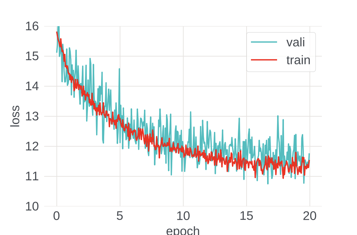
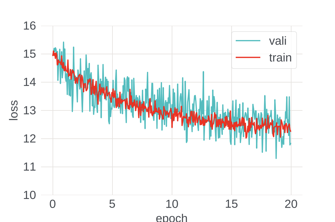
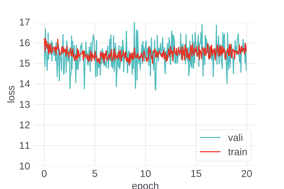
We compare the performance of our sparse models with DP-SGD, after hyperparameter tuning. With respect to privacy, we fix the same privacy parameters and for all the algorithms. For the RDP accountant [MTZ19], we choose the noise multiplier for DP-SGD. For the other sparse algorithms, we divide our privacy budget into two parts: and for noise addition, and for private selection. By Theorem 3, we set for our sparse algorithms. The hyperparameters for the algorithms are summarized in Table 1.
| DP-SGD | DP sparse | |
|---|---|---|
| Batch size | 20 | 20 |
| Learning rate | 0.001 | 0.001 |
| Epoch | 20 | 20 |
| First gradient clipping norm | 15 | 15 |
| First gradient clipping norm | 15 | 15 |
| Second gradient clipping norm | N/A | 1 |
| Sparsity parameter | N/A | 0.001 |
| DP selection clipping norm | N/A | 0.1 |
From Figure 1, we observe that our sparse algorithms have provided much better performance than DP-SGD, both in terms of the training error or test error. Furthermore, the private selection by the exponential mechanism slightly outperforms the sparse vector technique, which is consistent with the results in [LSL17].
One valid complaint is that our algorithms give extremely weak privacy guarantees, since is too large to be practical for most applications. We remark that this value is an upper bound on the privacy loss budget.
As mentioned in Section 5, our computation is quite conservative, and we believe that the true value should be much smaller. Here we justify our conjecture by an empirical method. Note that the gap between the training error and test error (generalization error) can serve as a lower bound on the privacy level, as shown in [DFH+15], and [JLN+20]. From Figure 1, we find that the generalization errors of both DP-SGD and our sparse algorithm are small that are consistent with good privacy guarantees. Furthermore, if we improve the noise multiplier of DP-SGD to the same level of our sparse algorithms (), we observe that the generalization errors are still comparable between our sparse algorithms (Figure 1(d) and Figure 1(e)) and DP-SGD (Figure 1(c)), indicating they share similar privacy guarantees. As a benchmark, non-private algorithm has provided the best training error and test error. However, the huge gap between the training and test error indicates the model has provided almost no privacy guarantees. Besides, the periodic behaviour in the training error also indicates the model has severely memorized the training dataset.
6.5 Evaluation for unintended memorization
In this section, we use another method to estimate the privacy level of our model. Specifically, we follow the Secret Sharer frameworks proposed from [CLE+19], which aims to measure the unintended memorization of rarely-occurring phrases in the dataset. This method has been further explored in recent works [JE19, RTM+20].
First, we randomly generate canaries, each containing three words. The reason we opt for inserting three-word canaries is that computing the ranks for longer canaries is time-consuming. Each word in a canary is uniformly randomly chosen from the 1K vocabulary. This is because we want to measure unintended memorization of our models, i.e., the memorization of atypical phrases in the language model, which is in fact orthogonal to our learning task. Two examples of our canaries are “mother government opportunity” and “prices effort me”.
Next, we insert all these canaries into random positions in our original dataset, each canary appearing exactly times. Then we train our models as before. Note that the canaries have a trivial impact on our models, since the cumulative number of inserted phrases is relatively small relative to the size of the original dataset.
We use the Random Sampling method, as proposed in [CLE+19], to measure whether the canary is memorized by our model. Specifically, for a canary , we define the log-perplexity of the model on as . We define the rank of the canary as , where is the vocabulary. Intuitively, a high rank indicates the model highly favors the canary as compared to random chance. In other words, the model has “memorized” the canary, suggesting a privacy violation. We note that when computing each canary’s rank, it is time-consuming to enumerate all the possible phrases. Therefore, we randomly pick up 10K phrases from the domain and compute ’s rank in the subset instead.
In Figure 2, we show the distributions of the rank when , and . We run the experiments as mentioned above with non-private algorithm, DP-SGD, and Algorithm 3 (instantiated with the exponential mechanism for private selection), where we use the same hyperparameters as in the previous experiments. Note that for DP-SGD and DP Sparse, we are using exactly the same noise parameter . The experiment is designed to validate the hypothesis that the trained models exhibit similar levels of unintended memorization.
As a benchmark, we randomly select phrases that are outside of the training dataset, and we plot the histogram of the rank in Figure 2(d). We find that it is very close to the uniform distribution (confirmed by the chi-squared goodness of fit test). This is indeed expected since the process is equivalent to uniformly randomly drawing one sample from an ordered set, since the phrase is independent of the trained model.
The top two rows of Figure 2 report results for small ( and 9, respectively). Unlike the non-private training, both DP-SGD and DP Sparse result in histograms close to the uniform distribution (Figures 2(b) and 2(c)).
We also compute the chi-squared distance, and the -values of Pearson’s chi-squared tests (Table 2). Where the -values are not statistically significant, the chi-squared test fails to reject the null hypothesis, i.e., that the training procedure preserves privacy. Visually, the non-private algorithm produces a histogram that is highly concentrated to the right, which indicates that the model has indeed memorized the training dataset. Therefore, we argue that our sparse algorithm gives comparable privacy guarantees as DP-SGD, which are much better than the non-private version.
Finally, this method can be part of hyperparameter tuning, where the chi-squared distance can be an excellent metric to measure privacy leakage. For the case of , we observe that Figure 2 is consistent with the empirical being quite small (ranging between and ), following the group property of differential privacy, and the fact that the uniform distribution breaks down at some place between and .
| non-private | DP-SGD | DP Sparse | random | |
| 2.62 (.00) | .007 (.63) | .005 (.85) | .005 (.86) | |
| 3.24 (.00) | .004 (.88) | .007 (.68) | .010 (.33) | |
| 3.27 (.00) | .011 (.31) | .026 (.00) | .002 (.98) |
7 Acknowledgements
The authors thank Milan Shen and Will Bullock for helpful suggestions and support for this work.
References
- [ACG+16] Martin Abadi, Andy Chu, Ian Goodfellow, H Brendan McMahan, Ilya Mironov, Kunal Talwar, and Li Zhang. Deep learning with differential privacy. In Proceedings of the 2016 ACM SIGSAC Conference on Computer and Communications Security, pages 308–318, 2016.
- [AMCDC18] Gergely Acs, Luca Melis, Claude Castelluccia, and Emiliano De Cristofaro. Differentially private mixture of generative neural networks. IEEE Transactions on Knowledge and Data Engineering, 31(6):1109–1121, 2018.
- [ASY+18] Naman Agarwal, Ananda Theertha Suresh, Felix Xinnan X Yu, Sanjiv Kumar, and Brendan McMahan. cpsgd: Communication-efficient and differentially-private distributed sgd. In Advances in Neural Information Processing Systems, pages 7564–7575, 2018.
- [AZK+18] Nazmiye Ceren Abay, Yan Zhou, Murat Kantarcioglu, Bhavani Thuraisingham, and Latanya Sweeney. Privacy preserving synthetic data release using deep learning. In Joint European Conference on Machine Learning and Knowledge Discovery in Databases, pages 510–526. Springer, 2018.
- [BBG18] Borja Balle, Gilles Barthe, and Marco Gaboardi. Privacy amplification by subsampling: Tight analyses via couplings and divergences. In Advances in Neural Information Processing Systems, pages 6277–6287, 2018.
- [BJWW+19] Brett K Beaulieu-Jones, Zhiwei Steven Wu, Chris Williams, Ran Lee, Sanjeev P Bhavnani, James Brian Byrd, and Casey S Greene. Privacy-preserving generative deep neural networks support clinical data sharing. Circulation: Cardiovascular Quality and Outcomes, 12(7):e005122, 2019.
- [BPS19] Eugene Bagdasaryan, Omid Poursaeed, and Vitaly Shmatikov. Differential privacy has disparate impact on model accuracy. In Advances in Neural Information Processing Systems, pages 15479–15488, 2019.
- [BST14] Raef Bassily, Adam Smith, and Abhradeep Thakurta. Private empirical risk minimization: Efficient algorithms and tight error bounds. In Proceedings of the 55th Annual IEEE Symposium on Foundations of Computer Science, FOCS ’14, pages 464–473, Washington, DC, USA, 2014. IEEE Computer Society.
- [CH11] Kamalika Chaudhuri and Daniel Hsu. Sample complexity bounds for differentially private learning. In Proceedings of the 24th Annual Conference on Learning Theory, COLT ’11, pages 155–186, 2011.
- [CLE+19] Nicholas Carlini, Chang Liu, Úlfar Erlingsson, Jernej Kos, and Dawn Song. The secret sharer: Evaluating and testing unintended memorization in neural networks. In 28th USENIX Security Symposium, pages 267–284, 2019.
- [CTW+20] Nicholas Carlini, Florian Tramer, Eric Wallace, Matthew Jagielski, Ariel Herbert-Voss, Katherine Lee, Adam Roberts, Tom Brown, Dawn Song, Ulfar Erlingsson, Alina Oprea, and Colin Raffel. Extracting training data from large language models, 2020.
- [CWZ19] T. Tony Cai, Yichen Wang, and Linjun Zhang. The cost of privacy: Optimal rates of convergence for parameter estimation with differential privacy. arXiv preprint arXiv:1902.04495, 2019.
- [CXX+18] Qingrong Chen, Chong Xiang, Minhui Xue, Bo Li, Nikita Borisov, Dali Kaarfar, and Haojin Zhu. Differentially private data generative models. arXiv preprint arXiv:1812.02274, 2018.
- [DFH+15] Cynthia Dwork, Vitaly Feldman, Moritz Hardt, Toniann Pitassi, Omer Reingold, and Aaron Leon Roth. Preserving statistical validity in adaptive data analysis. In Proceedings of the Forty-Seventh Annual ACM Symposium on Theory of Computing (STOC), page 117–126, 2015.
- [Dif17] Differential Privacy Team, Apple. Learning with privacy at scale. https://machinelearning.apple.com/docs/learning-with-privacy-at-scale/appledifferentialprivacysystem.pdf, December 2017.
- [DKY17] Bolin Ding, Janardhan Kulkarni, and Sergey Yekhanin. Collecting telemetry data privately. In Advances in Neural Information Processing Systems 30, NIPS ’17, pages 3571–3580. Curran Associates, Inc., 2017.
- [DMNS06] Cynthia Dwork, Frank McSherry, Kobbi Nissim, and Adam Smith. Calibrating noise to sensitivity in private data analysis. In Proceedings of the 3rd Conference on Theory of Cryptography, TCC ’06, pages 265–284, Berlin, Heidelberg, 2006. Springer.
- [DNR+09] Cynthia Dwork, Moni Naor, Omer Reingold, Guy N. Rothblum, and Salil Vadhan. On the complexity of differentially private data release: Efficient algorithms and hardness results. In Proceedings of the 41st Annual ACM Symposium on the Theory of Computing, STOC ’09, pages 381–390, New York, NY, USA, 2009. ACM.
- [DR14] Cynthia Dwork and Aaron Roth. The algorithmic foundations of differential privacy. Foundations and Trends in Machine Learning, 9(3–4):211–407, 2014.
- [DR19a] David Durfee and Ryan M Rogers. Practical differentially private top-k selection with pay-what-you-get composition. Advances in Neural Information Processing Systems, 32:3532–3542, 2019.
- [DR19b] David Durfee and Ryan M. Rogers. Practical differentially private top- selection with pay-what-you-get composition. In Advances in Neural Information Processing Systems, pages 3532–3542, 2019.
- [EPK14] Úlfar Erlingsson, Vasyl Pihur, and Aleksandra Korolova. RAPPOR: Randomized aggregatable privacy-preserving ordinal response. In Proceedings of the 2014 ACM Conference on Computer and Communications Security, CCS ’14, pages 1054–1067, New York, NY, USA, 2014. ACM.
- [FJR15] Matt Fredrikson, Somesh Jha, and Thomas Ristenpart. Model inversion attacks that exploit confidence information and basic countermeasures. In Proceedings of the 22nd ACM SIGSAC Conference on Computer and Communications Security, pages 1322–1333, 2015.
- [FK79] W Nelson Francis and Henry Kucera. Brown corpus manual. Letters to the Editor, 5(2):7, 1979.
- [GL13] Saeed Ghadimi and Guanghui Lan. Stochastic first-and zeroth-order methods for nonconvex stochastic programming. SIAM Journal on Optimization, 23(4):2341–2368, 2013.
- [HMNZ19] Meisam Hejazinia, Pavlos Mitsoulis-Ntompos, and Serena Zhang. Deep personalized re-targeting. In 2019 IEEE/ACM International Conference on Advances in Social Networks Analysis and Mining (ASONAM), pages 1148–1154. IEEE, 2019.
- [HSLH17] Yan Hu, Weisong Shi, Hong Li, and Xiaohui Hu. Mitigating data sparsity using similarity reinforcement-enhanced collaborative filtering. ACM Transactions on Internet Technology (TOIT), 17(3):1–20, 2017.
- [HT10] Moritz Hardt and Kunal Talwar. On the geometry of differential privacy. In Proceedings of the 42nd Annual ACM Symposium on the Theory of Computing, STOC ’10, pages 705–714, New York, NY, USA, 2010. ACM.
- [JE19] Bargav Jayaraman and David Evans. Evaluating differentially private machine learning in practice. In 28th USENIX Security Symposium, pages 1895–1912, 2019.
- [JLN+20] Christopher Jung, Katrina Ligett, Seth Neel, Aaron Roth, Saeed Sharifi-Malvajerdi, and Moshe Shenfeld. A new analysis of differential privacy’s generalization guarantees. In Thomas Vidick, editor, 11th Innovations in Theoretical Computer Science Conference, ITCS 2020, January 12-14, 2020, Seattle, Washington, USA, volume 151 of LIPIcs, pages 31:1–31:17, 2020.
- [JT14] Prateek Jain and Abhradeep Guha Thakurta. (Near) dimension independent risk bounds for differentially private learning. In International Conference on Machine Learning, pages 476–484, 2014.
- [KJ16] Shiva Prasad Kasiviswanathan and Hongxia Jin. Efficient private empirical risk minimization for high-dimensional learning. In International Conference on Machine Learning, pages 488–497, 2016.
- [KOV15] Peter Kairouz, Sewoong Oh, and Pramod Viswanath. The composition theorem for differential privacy. In International conference on machine learning, pages 1376–1385, 2015.
- [LK20] Jaewoo Lee and Daniel Kifer. Differentially private deep learning with direct feedback alignment. arXiv preprint arXiv:2010.03701, 2020.
- [LSL17] Min Lyu, Dong Su, and Ninghui Li. Understanding the sparse vector technique for differential privacy. Proceedings of the VLDB Endowment, 10(6), 2017.
- [MAM+18] Brendan McMahan, Galen Andrew, Ilya Mironov, Nicolas Papernot, Peter Kairouz, Steve Chien, and Úlfar Erlingsson. A general approach to adding differential privacy to iterative training procedures. 2018. Workshop on Privacy Preserving Machine Learning (NeurIPS 2018).
- [MCCD13] Tomas Mikolov, Kai Chen, Greg Corrado, and Jeffrey Dean. Efficient estimation of word representations in vector space. arXiv preprint arXiv:1301.3781, 2013.
- [MNHZB19] Pavlos Mitsoulis-Ntompos, Meisam Hejazinia, Serena Zhang, and Travis Brady. A simple deep personalized recommendation system. arXiv preprint arXiv:1906.11336, 2019.
- [MRTZ18] Brendan McMahan, Daniel Ramage, Kunal Talwar, and Li Zhang. Learning differentially private recurrent language models. In International Conference on Learning Representations (ICLR), 2018.
- [MSC+13] Tomas Mikolov, Ilya Sutskever, Kai Chen, Greg S Corrado, and Jeff Dean. Distributed representations of words and phrases and their compositionality. Advances in neural information processing systems, 26:3111–3119, 2013.
- [MT07] Frank McSherry and Kunal Talwar. Mechanism design via differential privacy. In Proceedings of the 48th Annual IEEE Symposium on Foundations of Computer Science, FOCS ’07, pages 94–103, Washington, DC, USA, 2007. IEEE Computer Society.
- [MTZ19] Ilya Mironov, Kunal Talwar, and Li Zhang. R’enyi differential privacy of the sampled gaussian mechanism. arXiv preprint arXiv:1908.10530, 2019.
- [Opa20] Introducing opacus: A high-speed library for training pytorch models with differential privacy. https://github.com/pytorch/opacus, August 2020.
- [PKP+18] Vadim Popov, Mikhail Kudinov, Irina Piontkovskaya, Petr Vytovtov, and Alex Nevidomsky. Distributed fine-tuning of language models on private data. In International Conference on Learning Representations, 2018.
- [PSM+18] Nicolas Papernot, Shuang Song, Ilya Mironov, Ananth Raghunathan, Kunal Talwar, and Ulfar Erlingsson. Scalable private learning with PATE. In International Conference on Learning Representations, 2018.
- [RTM+20] Swaroop Ramaswamy, Om Thakkar, Rajiv Mathews, Galen Andrew, H Brendan McMahan, and Françoise Beaufays. Training production language models without memorizing user data. arXiv preprint arXiv:2009.10031, 2020.
- [SS15] Reza Shokri and Vitaly Shmatikov. Privacy-preserving deep learning. In Proceedings of the 22nd ACM SIGSAC conference on computer and communications security, pages 1310–1321, 2015.
- [SU17] Thomas Steinke and Jonathan Ullman. Tight lower bounds for differentially private selection. In Proceedings of the 58th Annual IEEE Symposium on Foundations of Computer Science, FOCS ’17, pages 552–563, Washington, DC, USA, 2017. IEEE Computer Society.
- [TAM19] Om Thakkar, Galen Andrew, and H Brendan McMahan. Differentially private learning with adaptive clipping. arXiv preprint arXiv:1905.03871, 2019.
- [TTZ15] Kunal Talwar, Abhradeep Thakurta, and Li Zhang. Nearly-optimal private LASSO. In Advances in Neural Information Processing Systems 28, NIPS ’15, pages 3025–3033. Curran Associates, Inc., 2015.
- [VTJ19] XS Vu, SN Tran, and L Jiang. dpugc: Learn differentially private representation for user generated contents. In Proceedings of the 20th International Conference on Computational Linguistics and Intelligent Text Processing, pages 1–16, 2019.
- [WBK19] Yu-Xiang Wang, Borja Balle, and Shiva Prasad Kasiviswanathan. Subsampled Rényi differential privacy and analytical moments accountant. In The 22nd International Conference on Artificial Intelligence and Statistics, pages 1226–1235. PMLR, 2019.
- [WCX19] Di Wang, Changyou Chen, and Jinhui Xu. Differentially private empirical risk minimization with non-convex loss functions. In International Conference on Machine Learning, pages 6526–6535. PMLR, 2019.
- [WJEG19] Lingxiao Wang, Bargav Jayaraman, David Evans, and Quanquan Gu. Efficient privacy-preserving nonconvex optimization. arXiv preprint arXiv:1910.13659, 2019.
- [WYX17] Di Wang, Minwei Ye, and Jinhui Xu. Differentially private empirical risk minimization revisited: Faster and more general. In Advances in Neural Information Processing Systems, volume 30, pages 2722–2731. Curran Associates, Inc., 2017.
- [ZWB20] Yingxue Zhou, Zhiwei Steven Wu, and Arindam Banerjee. Bypassing the ambient dimension: Private SGD with gradient subspace identification. arXiv preprint arXiv:2007.03813, 2020.
- [ZZMW17] Jiaqi Zhang, Kai Zheng, Wenlong Mou, and Liwei Wang. Efficient private erm for smooth objectives. In IJCAI, 2017.
Appendix A Proof of Lemma 6
The first half comes from [ASY+18]. Therefore, it is enough to prove the second half, where we use a similar proof technique with [ASY+18] and [GL13].
First observe that, for any ,
where we define .
By the convexity and smoothness, we have
Combining these, for all ,
where the last inequality uses the convexity and the fact that .
Summing up the above inequalities and re-arranging the terms, we have
Taking the expectation on both sides, we have
We first bound the third term in the parenthesis. According to the definition of in Lemma 6, we have
| (2) |
With respect to the second term,
Note that
where the last equality comes from the fact that is an unbiased estimator of .
By taking , we have , , and . Therefore, by combining them,