Hamiltonian dynamics is given in the two dimensional phase space $(x,p)$, with a single Hamiltonian $H$;

Nambu generalized this to D-dim phase space $(x_{1},x_{2},\cdots,x_{D})$ with D$-$1 Hamiltonians $(H_{1},H_{2},\cdots,H_{D-1})$;

where the r.h.s. is Jacobian, called “Nambu bracket”:

Liouville theorem that the phase space volume is unchanged gives incompressible fluid. The peculiar “advective term”, an origin of non-linearity in hydrodynamics, appears naturally in Nambu dynamics;

since it gives $\dot{v^{i}}=({\bf v}\cdot{\bf\nabla})v_{i}$.

Hamiltonians are equal to the stream functions in hydrodynamics $\{\psi_{1},\psi_{2},\cdots,\psi_{D-1}\}$

which implies $\bm{\nabla\cdot v}=0$, and the velocity points along the intersection line of all the stream functions be constant.

Navier-Stokes equation for incompressive fluid reads

where $p$ is pressure, $\mu$ is shear viscosity with dimension [Pas][s]. We also use $\nu=\mu/\rho$ with dimension [$m^{2}$/s]. $V(x)$ is an external potential of force.

The r.h.s. (force term) can also be written by using Nambu brackets:

In his last work, Nambu proposed “the quantization of space” (2011, 2013), or the introduction of non-commutative space in hydrodynamics [2]. His intension is to understand the empirical “Bode law”, that is, the radius of the n-th planet follows $R_{n}=a\;2^{n}+b$.

We [SaBSu(2014)] interpreted his hydrodynamics as “Hydrodynamics of Granular Material”[3].

To quantize the Nambu bracket, we can use the Moyal product, familiar for non-commutative space. For D=2, 3 hydrodynamics, the Moyal products are given by

Therefore, the quantization is carried out by replacing

and

The Planck constant in our case is the minimum area $\theta_{2}$ in 2D and minimum volume $\theta_{3}$ in 3D of a granular particle which are identified as the particle size.

Then, the additional force $K$ appears, as the finite size effect or the quantum effect of fluid particle,

where $(\psi_{1}(x),\psi_{2}(x))$ are stream functions.

Next, we perform the hydrodynamic simulation in 2D [KaKuNaSaSu(2018)][4].

Fluid flows from the left to the right inside a canal; with a table-shaped obstacle making a upper small and a lower large slits.

Let look at two movies 1 and 2 ²² 2 http://www2.yukawa.kyoto-u.ac.jp/~mayumi.saitou/simulation.html:

1) The size of a canal and an obstacle: 64[cm] (length) $\times$ 21[cm] (width) with small slit=2[cm] and large slit=8[cm], the obstacle size is 4[cm] (width) $\times$ 11[cm] (hight : including semicircles in both sides). Total number of grid point on the canal is 175 $\times$ 71, the minimum size of the grid length is 0.167[cm].

2) A time step is 0.001[s]; totally 2,000[s]. Reynolds number(Re)=700, $\rho=10^{3}[kg/m^{3}],\eta=8.85\times 10^{-4}[Pa][s]$, and a typical velocity is $U_{0}=0.55[cm/s]$.

3) Characteristics of the 1st and the 2nd movies:

[movie 1] (commutative space with zero particle size) Before1000[s], vortices are generated periodically; at 1025 [s] “blue” (anticlockwise vortex) region and “red” (clockwise vortex) region merges to form “two attached eddies”; at 2000[s] flow is stabilized.

[movie 2] (non-commutative space with non-zero particle size) No active periodic production of vortices just after the obstacle, but is active at down stream; “two attached eddies” appear from the beginning; after 1300[s] flow is stabilized.

It is important to note that Nambu’s (hydro-)dynamics in D-dim phase space is equal to the dynamics of (D-2)-dim extended object (D-2)-brane; D=2: particle; D=3: string [Nambu(1980)]; D=4: membrane [Su(1983)]; in general (Takhatajan(1994)] [5] ³³ 3 This section started non-relativistically in the talk, so that there is a gap between this non-realtivistic treatment and the relativistic ones in the following sections. To fill the gap, please follow Nambu and Sugamoto who studied relativistic hydrodynamics with 2-form and 3-form momenta, $p_{\mu\nu}$ and $p_{\mu\nu\rho}$. Then, the non-relativistic 3D acton Eq.(15) can be generalized relativistically as $S^{\prime}_{3}=\int p_{\mu\nu}\;dX^{\mu}\wedge dX^{\nu}+\cdots$, including $\mu,\nu=0$. In deriving the actions, they used the Hamilton-Jacobi (H-J) formalism. The reason is as follows: The H-J is a method to give two actions, differing by total derivatives (or p-forms). They are usually identical, giving the canonical transformation, but sometimes differ due to the non-integrable phase factors. Therefore, Clebsch theory and gauge theories (with p-forms) in general fits to the H-J.

For example, 3D hydrodynaics in (X, Y, Z) phase space can be described by

Its equation of motion reads Nambu dynamics:

This is a generalization of the usual 2D phase space $(x,p)$ case of $S_{2}=\int pdx-\psi_{1}dt$.

Here, time t in 2D becomes “area A” in 3D, namely,

World sheet of string sweeps in (Y, Z), moving in t and parametrized by $(0\leq\sigma\leq 2\pi)$; X is the momentum.

Path integration with weights, $e^{\frac{i}{\hbar}S_{2}}~\mathrm{and}~e^{\frac{i}{\theta_{3}}S_{3}}$, gives quantum mechanics:

$\hat{p}=-i\hbar\frac{\partial}{\partial x},~\mathrm{and}~\frac{\partial}{\partial x}x=1$ for 2D, while for 3D we have

The derivative in 3D is replaced by the functional derivative (in tangential t and normal direction $\mu$):

Now, we have the uncertainty relation in 2D and 3D (see Appendix 2)):

Now, QED and its analog in 3D hydrodynamics read

This is the Schild gauge string theory, coupled to Kalb- Ramond field ⁴⁴ 4 A gap exists again between $S_{\mathrm{string}}$ and $S_{\mathrm{Schild}}$. To fill the gap, please write the former action in terms of $X^{\mu}$ (including $\mu=0$):

where $m$ can be $(\theta_{3})^{1/3}$ and the string tension $\theta_{3}^{-2/3}$.

Our uncertainty relation to give the minimum size for a granular particle is equal to the space-time uncertainty principle claimed by Yoneya [Yoneya(1997)] [6].

$\bullet$ (i, 0) components of Kalb-Ramond field: The wave equation, describing the flow of fluid is

which is equal to the “gauge symmetry of string” in (i, 0) directions:

Therefore, $gW_{i0}(x)=\psi_{1}\frac{\partial}{\partial x^{i}}\psi_{2}$, and the vortex interaction is mediated by the stream functions, or equivalently by (i, 0) component Kalb-Ramond fields.

(see H. Lamb “Hydrodynamics”[7], a favorite book of Nambu. He kept reading it until his death.)

Clebsch started with ${\bf v}=-{\bf\nabla}\phi(x)+\lambda(x){\bf\nabla}\mu(x)$, then $\bm{\omega}=\bm{\nabla}\times\bm{v}=\{\bm{x},\lambda,\mu\}_{NB}={\bf\nabla}\lambda\times{\bf\nabla}\mu$; while Nambu started with ${\bf v}=\{{\bf x},\psi_{1},\psi_{2}\}_{NB}={\bf\nabla}\psi_{1}\times{\bf\nabla}\psi_{2}$.

Nambu and Clebsch are “dually” related, under $(v)\leftrightarrow(\omega)$, and (stream functions) $\leftrightarrow$ functions $(\lambda,\ \mu)$.

Nambu studied the flow along velocity $(v)$, while Clebsch studied the flow along vorticity $(\omega)$.

Consider “string=vortex line or tube”, stretching in $\sigma$ direction, parallel to vorticity $\omega$,

Clebsch easily shows the vorticity theorem by Helmholtz, and also considered the reparametrization transformation $(\sigma,t)\rightarrow(\sigma^{\prime},t^{\prime})$.

This duality is probably “T-duality” (translational mode $\leftrightarrow$ winding mode) in string theory; suggesting a duality in hydrodynamics.

This model was given 40 years ago by Nambu (1977) and by one of the authors (A.S). [Su(1979), Seo-Okawa-Su(1979,1981)] [8].

This Nambu’s relativistic hydrodynamics be Kalb-Ramod theory coupled with vorticity source:

where $W_{\mu\nu}$ is Kalb-Ramond field (1973) (now called B-field or anti-symmetric tensor field), and $V^{\mu}(x)$: fluid velocity, and $\omega^{\mu\nu}(x)$: vorticity source. Then, the realtivistic fluid velocity satisfies the continuity relation naturally, $\sum_{\mu=0}^{3}\partial_{\mu}V^{\mu}=0$.

$\bullet$ A filament of vortex line, extending in Z direction with circulation $\gamma$, gives

so that

$\bullet$ Kalb-Ramond field is a “gauge field” in string. This gauge symmetry is called “Kalb-Ramond symmetry”:

The hybrid model describes the interaction of vortex strings through the fluid field (K-R field):

This is very similar to QED in which electric current couples to photon. That is, in hydrodynamics, the interaction of vortices with fluid can be represented by the coupling of current of string to K-R field:

Understanding of power spectrum of high energy cosmic ray (having Knee and Ankle) can be applicable to power spectrum of vortices?

$\bullet$ An example of string field in the ordinary case: Since $\Psi[C,A]\approx\Psi[{\bf X}(\sigma,t)]$, the mode expansion $X^{i}(\sigma,t)=x^{i}+\frac{\kappa}{\pi}(p^{i}t)+i\sqrt{\frac{\kappa}{4\pi}}\sum_{k\neq 0}\left(x^{i}_{k}e^{-ik(t-\sigma)}+\tilde{x}^{i}_{k}e^{-ik(t+\sigma)}\right),~(\kappa=(\theta_{3})^{2/3})$, gives the functional derivative

Then, the wave equation reads

$\bullet$ String has, in addition to the translational mode, the k-th oscillation mode in the i-th direction with occupation number $\{n^{i}_{k}\}$. The wave functional becomes

where $\hat{A}_{p,\{n^{i}_{k}\}}$ and $\hat{\tilde{A}}_{p,\{\tilde{n}^{i}_{k}\}}$ are annihilation operator of string itself of right- and left-moving, respectively. Here, we have to choose a proper string theory (not necessary to follow the usual examples) so as to reproduce the vortex production rate in a given hydrodynamics.

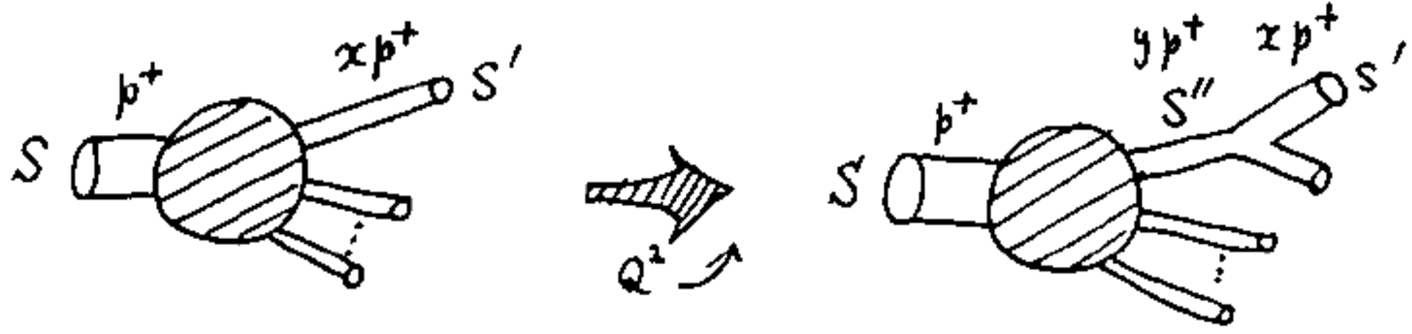
A nucleon is composed of quarks and gluons (partons); having momentum fraction x relative to P of the nucleon. Patrons are probed by photon $\gamma$, with momentum Q. If $Q^{2}$ is increased, the finer structure reveals:

Similarly, a turbulence is composed of vortices (partons) with various sizes and shapes,

The evolution for closed string (vortex) was given 30 years ago by us [MaruiOdaSu(1990)], in a similar manner as the Altarelli and Parisi (1973) equation in QCD [9].

Distribution function $D_{S^{\prime}S}(x,Q^{2})$ of string $S^{\prime}$ inside $S^{\prime}$ with momentum fraction $x$ at the energy scale $Q^{2}$ satisfies

where the splitting function is given in Figure 6.

Using the light-cone field theory of string by Mandelstam (1973) and Kaku-Kikkawa (1974) [10], we obtain

which differs from the usual distribution functions of quarks and gluons,

$\star$ Note: The concept itself is applicable to the turbulence or other vortex phenomena, but we have to choose the more proper string theory (not necessary the usual ones), so that it may reproduce the realistic phenomena in a given hydrodynamics.

Shear viscosity $\eta,~(\eta/\rho=\nu)$ introduces diffusion in velocity field: $\dot{\bm{v}}=\Delta\bm{v}$ (constitutive equation). To include the thermal fluctuations at finite temperature the “constitutive equation” is relaxed by the fluctuation of force, following the Gaussian distribution with width proportional to $T$:

In thermodynamics, $\xi$ plays the same role as the momentum $p$ in quantum mechanics, and hence

We can include the dissipation effects also in string theory, following for example [Aibara et al.(2019)] [11]. In the particle theory we have

under the constraint of $\dot{\bm{x}}=\bm{v}$, or $\left(-i\hbar\bm{\nabla}_{x}+g\bm{A}(\bm{x})-m\bm{v}\right)\psi(\bm{x},\bm{v},t)=0.$

The corresponding equation in string is

with a constraint, representing

where $\frac{\partial C^{t\mu}}{\partial A}(x)=D^{t\mu}(x)$, and $C^{t\mu}=X^{t}\wedge X^{\mu}$.

4D Energy momentum tensor in particle thery $T^{\mu\nu}(x)=\frac{\partial\mathcal{L}}{\partial(\partial_{\mu}\phi(x))}\partial^{\nu}\phi(x)-g^{\mu\nu}(x)\mathcal{L}$ becomes in string

Oscillations give various “strain” to string

Therefore, the derivative expansion is surely modified ?

1. (1)

   Nambu’s hydrodynamics in non-commutative space can be the hydrodynamics of granular material.

2. (2)

   The non-commutativity (or quantization) of space can be introduced, by 1) Moyal product, 2) vortex as string and its coupling to Kalb-Ramond field, or 3) string field theory.

3. (3)

   In applying the string field theory, 1) evolution equation describing the change of energy scale, and 2) Landau’s way of derivative expansion of energy momentum tensor, can be applied.

4. (4)

   Note however: We have to find a proper string theory so as to reproduce a given hydrodynamics.

5. (5)

   Force from the stress tensor should be re-examined.

The authors give their sincere thanks to Professor Yasuhide Fukumoto and Professor Hiroshi Itoyama for inviting one of them (A.S.) to the workshop, where very active discussions were exchanged between the participants. Especially, we are grateful to Yutaka Matsuo for clarifying a number of unclear points in their talk during and after the workshop, which triggers a new insight by Yutaka Matsuo and A.S. to appear in the proceedings.

This work was partly supported by Osaka City University Advanced Mathematical Institute (MEXT Joint Usage/Research Center on Mathematics and Theoretical Physics JPMXP0619217849). Numerical computation in this work was carried out at the Yukawa Institute Computer Facility.

=============================================

(A1-1) : The fractional step method with a tentative $v*$ is used:

Applying the continuity condition for $v_{i}^{(n+1)}$, $p$ can be determined by ${\color[rgb]{0,0,0}{\Delta p}}=\frac{\rho}{\Delta t}\ \nabla\cdot\bm{v}^{*}$.

(A1-2): “The 3rd order upwind difference” is used for the advective term.

(A1-3): About the boundary conditions, since the differential equations are the 3rd order ones, we impose, 1) $\bm{v}=\bm{0},~(\bm{\nabla}p)_{\bot}=\bm{0},~\bm{K}_{\bot}=\bm{0}$ on the boundary, 2) $(\bm{\nabla}p)_{\bot}=\bm{0}$ at the entrance, and 3) $p=0$ at the exit.

See Feynman’s paper (1948), and

insert $\frac{\partial O(\bm{X}(\sigma)}{\partial t}$ and $\frac{\delta A^{23}[C(\sigma)]}{\delta C(\sigma)}$ at the star, and perform integration by parts. Then we have $i\theta_{3}\;\frac{\partial O(\bm{X}(\sigma)}{\partial t}=[O(\bm{X}(\sigma),\oint\psi_{1}d\psi_{2}]$, and $i\theta_{3}\delta(\sigma-\sigma^{\prime})=[A^{23}(\sigma,t),X^{1}((\sigma^{\prime},t)]$, in the same manner as Feynman did for $\frac{dO(t)}{dt}~\mathrm{and}~\frac{dx(t)}{dx}$.

Without viscosity $\bm{v}=\bm{\nabla}\times\bm{\psi}$, we have a constant $\bm{\nabla}\cdot\bm{\psi}$, and $\bm{\omega}=\bm{\nabla}\times\bm{v}=-\Delta\bm{\psi}$. Then, in hydrodynamics

while in QED:

Now we can understand that attraction and repulsion is the same for electric charge and vortex, but is reversal for electric current.

In the hybrid model of hydrodynamics, vortex interaction is mediated by the Kalb-Ramond field:

with the components

Now, the vortex interaction is correctly reproduced:

The vortex interaction is mediated by $e(x)$ which are the Kalb-Ramond fields or the stream functions: $e^{i}(x)=W^{0i}=\psi^{i}(x)$.

$\bullet$ As we know that the massless modes of closed string in our simple case are dilation (D), graviton (G) and Kalb-Ramond (W) fields.

in the first quantized notation, that is,

References

• [1] Nambu dymamics: Y. Nambu, Phys. Rev. D7 (1973) 2405.
• [2] Nambu’s last work: Y. Nambu, Talk at International Workshop: Extra Dimensions
in the Era of the LHC, Dec. 12-14 (2011). https://sites.google.com/a/hetmail.phys.sci.osaka-u.ac.jp/edlhc11/;
Y. Nambu, Talk at Int. Symposium on Research Frontiers on Physics, Earth and Space Science, Dec. 17-18 (2013). http://thmat8.ess.sci.osaka-u.ac.jp/Meeting2013/Talks/YN.pdf
• [3] Hydrodynamics of granular material: M. Saitou, K. Bamba and A. Sugamoto: PTEP 103B03 (2014); M. Saitou: phD thesis, Ochanomizu U., March (2016).
• [4] Hydrodynamic simulation: T. Kawamura, A. Kuwana, Y. Nagata, M. Saitou and A. Sugamoto, PTEP 063J01(2018); T. Kawamura, A. Kuwana, M. Saitou, A. Sugamoto, Y. Nagata, RIMS Kokyuroku (2019), 2117:35-43. http://hdl.handle.net/2433/252120
• [5] Action of Nambu dynamics: Y. Nambu: Phys. Lett. 92B, 327 (1980); A. Sugamoto: Nucl. Phys. B215, 381 (1983); L. Takhtajan: Commun. Math. Phys. 160, 295 (1994).
• [6] Space time uncertainty principle: T. Yoneya, PTP 97, 949 (1997).
• [7] Clebsch’s work (1857,1859): referred in “Hydrodynamics” by Horace Lamb, Cambridge U. Press (1916).
• [8] Hybrid model of hydrodynamics: M. Kalb and P. Ramond, Phys. Rev. D9 (1974) 2273; Y. Nambu: “Quark Confinement and Field Theory”, eds. D. R. Stump and D. H. Weingarten, John Wiley and Sons (1977) 1; A. Sugamoto: Phys. Rev. D19 (1979) 1820; K. Seo and A. Sugamoto: Phys. Rev. D19 (1979) 3744; i.b.d. D24 (1981) 1630; A. Sugamoto, Lecture at Kashikojima Summer Institute, “Old Fashioned Duality Revisited”, arXiv: hep-th/9611051 (1996); R. Endo, K. Seo, A. Sugamoto, Grav. Cosmol. 8 (2002) 56.
• [9] Evolution equation of QCD and string: (QCD) G. Altarelli and G. Parisi, Nucl. Phys. B126 (1977) 298; (string) M. Marui, I. Oda, and A. Sugamoto, Int. J. Mod. Phys. A5 (1990) 4257; A. Sugamoto, Proceedings of the Trieste conference on “Supermembrane and Physics in 2+1 Dimensions” (1989).
• [10] String field theory: S. Mandelstam, Nucl. Phys. B64 (1973) 205; i.b.d.B69 (1974) 77; M. Kaku and K. Kikkawa, Phys. Rev. D10 (1974) 1110, 1823.
• [11] Non-equilibrium thermodynamics: N. Aibara, N. Fujimoto, S. Katagiri, M. Saitou, A. Sugamoto, T. Yamamoto, and T. Yumibayashi, PTEP 073A02 (2019).
• [12] Landau’s fluid dynamics: Sec.XV “Relativistic Fluid Dynamics” in “Fluid Mechanics” by L. Landau and E. M. Lifshitz.
• [13] R. P. Feynman, Rev. Mod. Phys. 20, 367 (1948).
• [14] J. Dulan, “Physics of granuler material” (1997) Editoins Eyrolles, Paris, translated in Japanese by Shu Nakanishi and Ko Okumura, (2001) Yoshioka-Shoten.