A Secure Sensor Fusion Framework for Connected and Automated Vehicles under Sensor Attacks

Our transportation systems are enhancing its intelligence with the surge of connected and automated vehicles (CAVs). With the increasing connectivity and automation, CAVs are expected to provide a safer, more efficient and environmentally friendly transportation systems [1][2]. Compared with traditional ones, CAVs use a variety of sensors to measure the surroundings so that various driving tasks such as lane keeping, collision avoidance, and vehicle following can be fulfilled. Moreover, taking the advantage of wireless communications, CAVs are now able to share their local sensor information with the surrounding vehicles and roadside units to increase traffic efficiency, safety or form vehicle platoonings. Therefore, the accuracy of the on-board sensors has to be guaranteed to achieve safe and secure driving and anomalous sensor values which result from malicious cyberattacks or faulty sensors can lead to severe consequences or fatalities in the worst case [3]. However, sensors of CAVs might be designed without security considerations and hence remain vulnerable to adversarial attacks. For instance, in [4], a self-driving vehicle based on LiDAR was compromised remotely by an attacker who generates more echoes of objects and vehicles. In [5], the authors investigate the vulnerabilities of millimeter-wave radars, ultrasonic sensors and forward-looking cameras to attacks and show that off-the-shelf hardware can be used to perform jamming and spoofing attacks on a Tesla Model S automobile. It has been shown in [6] that inexpensive commodity hardware can be used to perform various types of attacks, e.g., blinding, jamming, replay and spoofing attacks on camera and LiDAR systems. This shows that we need strategic countermeasures for identifying and dealing with sensor attacks on CAVs.

Security and privacy problems for general cyber-physical systems under sensor attacks have been addressed using various methodologies [7] -[14]. Traditional works on autonomous vehicles security focus on the cryptography part, e.g., designing new protocols for device authentication and data transmission [15, 16]. There are only a few results addressing and solving the problem of quantifying (minimizing) the performance degradation induced by attacks on CAVs. In [17, 18], the authors exploit sensor redundancy and provide detection and isolation algorithms for a single vehicle under sensor attacks. The problem of achieving consensus against replay attacks in an operator-vehicle network is solved in [19]. A control scheme is provided in [20] for a vehicle platoon whose communication network, DSRC, is under Denial-of-Service (DoS) attack. In [21], suitable countermeasures to detect replay attack for connected vehicles are provided. The authors of [22] provide an algorithm for detecting sensor attacks on connected vehicles using a set-membership filtering technique. The problem of attack detection and estimation for connected vehicles under sensor attacks is solved using an unbiased finite implulse response (UFIR) estimator in [23]. Shoukry et al. [24] suggest randomly turning off the transmitter for detecting attacks on LiDARs, which however may degrade system performance. Attack-resilient sensor fusion algorithms for cyber-physical systems are proposed in [25][26], where multiple so-called abstract sensors are used to measure the same physical variable and some of them are under attacks. Each abstract sensor provides a set with all possible values for the true state of the variable for the fusion algorithm, and then an attack-free fused measurement is obtained by checking the intersections of these sets. We provide a secure sensor fusion framework for CAVs under sensor attacks, where noise on sensor measurements is assumed to be bounded with unknown bounds, which might be applicable to a large class of security-critical CPSs.

Our sensor fusion approach is inspired by the work in [10], where the problem of state estimation for continuous-time linear time-invariant (LTI) systems is addressed. The authors propose a way of constructing an estimator using a bank of Luenberger observers, that provides a robust state estimation despite the fact that sensor attacks are present. The main idea of their estimation scheme is to place redundant sensors in the system. Sensor redundancy has been proved to be crucial for estimation under attacks [27, 10, 28, 29, 14, 30]. Using redundant sensors/actuators for secure estimation and control is a commonly adopted technique, see, e.g., [27, 10, 28, 29, 11, 31], and references therein. Note that it might be costly to create redundancy, which indicates some of these estimation methods might have conservative applications; however, for security-critical systems, for instance, CAVs, this is the price to pay [6].

In this manuscript, exploiting sensor redundancy, we address the problem of robust sensor fusion, attack detection and isolation, and control for a Cooperative Adaptive Cruise Control (CACC) equipped CAV in a vehicle platoon under sensor attacks. Assuming each vehicle in the platoon is equipped with multiple on-board sensors that measure the same physical variable, we consider the case where all the sensor measurements are subject to bounded noise with unknown bounds and the adversary has limited capability such that only less than half of the sensors are compromised. We assume that the set of attacked sensors are not a priori known to us and can be time-varying. For instance, the time-variance of the set of attacked sensors may be caused by the attack strategy adopted by the attacker with energy-saving considerations [32]. For every subset of sensors, we compute the largest difference between the average value of all the sensor measurements and the measurement of every single sensor in the subset. Then we select the sensors that lead to the smallest difference. If some of the sensors are under attacks, their measurements produces larger difference than the attack-free ones, in general and hence will not be used by the algorithm for estimation. Our fusion algorithm provides estimation errors that are bounded independent of the attack signals. Once we have an attack-free measurement, we provide algorithms for detecting and isolating the attacked sensors under the condition that the noise bounds are known. Finally, for each vehicle in the vehicular platoon, we provide a robust CACC scheme that stabilizes its closed-loop dynamics while minimizing the joint effect of estimation errors and channel noise on the platooning string-stable behavior as well as the tracking performance of each vehicle. Our controller design method is an extension of the results given in [33] by assuming system disturbances are present. In the case of cyberattacks, we show that a separation principle between sensor fusion and control holds and the vehicle platoon can be stabilized by closing the loop with the fusion algorithm and the robust controller. We conclude on stability of the closed-loop dynamics of each vehicle in the platoon from Input-to-State Stability (ISS) [34] of the closed-loop system with respect to the bounded estimation error. The performance of our methods is illustrated in several numerical examples.

The paper is organized as follows. In Section II, some preliminary results needed for the subsequent sections are presented. In Section III, we describe the vehicle platoon system we consider. In Section IV, we show that our fusion scheme provides robust estimates of the sensor measurements despite sensor attacks. In Section V, algorithms for detecting and isolating sensor attacks are presented. The proposed robust CACC scheme and stability analysis are given in Section VI. Simulation results are shown in Section VII. Finally, in Section VIII, concluding remarks are given.

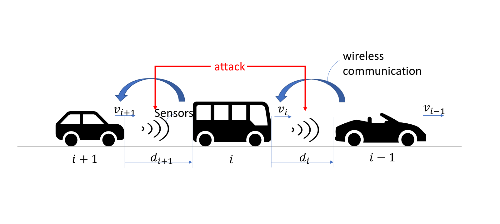
Consider a platoon of $m$ vehicles, shown in Figure 1. Denote the distance between vehicle $i$ and its preceding vehicle $i-1$ as $d_{i}$, and its velocity as $v_{i}$. The objective of each vehicle is to keep a desired distance with its preceding vehicle:

where $h_{i}$ represents the time headway of the $i$-th vehicle, $r_{i}$ is the standstill distance. $S_{m}=\left\{i\in\mathbb{N}|1\leq i\leq m\right\}$ denotes the set of all vehicles in a platoon of length $m\in\mathbb{N}$. The spacing policy adopted here is expected to improve string stability [36, 33]. The spacing error $e_{i}(t)$ is then defined as

where $q_{i}$ denotes the rear-bumper position of vehicle $i$ and $L_{i}$ denotes its length. We consider the following vehicle model adopted in [37],

with $\tau_{i}$ being a time constant representing driveline dynamics of vehicle $i$. $a_{i}$ is the acceleration of vehicle $i$; $u_{i}$ is the desired accelerations of vehicles $i$. We adopt the controller described in [37], where a new input $\xi_{i}$ is defined such that

with $\xi_{i}$ given as follows:

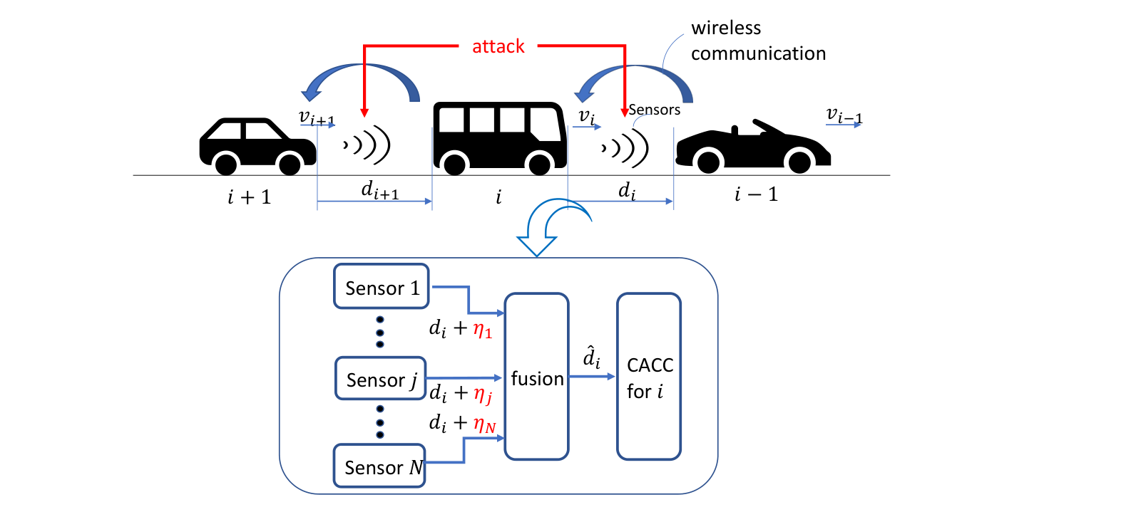
The feedforward term $u_{i-1}$ is transmitted from vehicle $i-1$ to vehicle $i$ through wireless communication channels. $v_{i}$ is measured by a wheel speed sensor of vehicle $i$, $a_{i}$ is measured by its accelerator. $d_{i}$ is measured by e.g, an ultrasonic sensor, a LiDAR, a radar, or a vision sensor.

Compared with the wheel speed sensor and the accelerator, which might require attackers’ physical access to be compromised, these sensors that measure $d_{i}$ are more exposed to the adversarial environment as they can be attacked from a distance [38, 39, 6, 5]. Therefore, we assume each vehicle in the platoon is equipped with $N$ different on-board sensors for measuring $d_{i}$, i.e., at every time $t$, vehicle $i$ has $N$ different measurements of $d_{i}(t)$. These measurements can be provided by a combination of various types of sensors, e.g., a combination of an ultrasonic sensor, a milimeter wave radar and a LiDAR, or multiple same type of sensors, e.g., multiple radars, or multiple LiDARs with different wavelengths etc.. Then, we assume $q$ ($q<N$) measurements are under attacks:

where $\nu_{i}\in\mathbb{R}$ and $\left\{\nu_{i}(t)\right\}\in l_{\infty}$ denotes measurement noise in each sensor, and $\eta\in\mathbb{R}^{N}$ denotes the vector of attack, i.e., if the $i$-th sensor is compromised, then $\eta_{i}(t)\neq 0$ for some $t\geq 0$; otherwise $\eta_{i}(t)=0$ for all $t\geq 0$. Let $W(t)\subset\left\{1,\ldots,N\right\}$ represent the unknown set of attacked sensors at time $t$, i.e.,

We assume an attacker attacks a sensor by modifying its measurement to any arbitrary value.

This definition means that if $d_{i}(t)$ is reconstructible from $D(t)$ under $q$ attacks, then there do not exist two distinct values $d_{i}(t)$ and $\bar{d}_{i}(t)$ that can explain the received data with less than $q$ sensors attacked, hence $d_{i}(t)$ can be reconstructed unambiguously.

Proof:

1) if: Suppose that $q<\frac{N}{2}$. For all $\eta_{a}(t)$ and $\eta_{b}(t)$ with $\card(\supp(\eta_{a}(t)))\leq q$ and $\card(\supp(\eta_{b})(t))\leq q$ and $t\geq 0$, the nonzero elements of $\eta_{b}(t)-\eta_{a}(t)$ cannot exceed $2q$, which is strictly smaller than $N$. Therefore, there do not exist $\eta_{a}(t)\neq\eta_{b}(t)$ such that

for any $t\geq 0$, since the number of nonzero elements on the right side of (10) is equal to $N$. Therefore, there do not exist $d_{i}(t)\neq\bar{d}_{i}(t)$ such that

for any $t\geq 0$, which indicates $d_{i}(t)$ is reconstructible from $D(t)$ for all $t\geq 0$.

2) only if: We prove by contrapositive. Suppose $q\geq\frac{N}{2}$, then for all $W_{a}(t)\subset\left\{1,\ldots,N\right\}$, with $\card(W_{a}(t))=q$ and $t\geq 0$, there must exist another set $W_{b}(t)\subset\left\{1,\ldots,N\right\}$ with $\card(W_{b}(t))=q$ such that $W_{b}(t)\cup W_{a}(t)=\left\{1,\ldots,N\right\}$ since $2q\geq N$. Let $I_{ab}(t)=W_{a}(t)\cap W_{b}(t)$. For all $d_{i}(t)\neq\bar{d}_{i}(t)$ and $t\geq 0$, we choose

then (11) holds with $d_{i}(t)\neq\bar{d}_{i}(t)$ for all $t\geq 0$, which indicates

with $d_{i}(t)\neq\bar{d}_{i}(t)$ for all $t\geq 0$. This contradicts the statement that $d_{i}(t)$ is reconstructible from $D(t)$ under $q$ attacks for all $t\geq 0$. $\blacksquare$.

For every subset $J\subset\left\{1,\ldots,N\right\}$ sensors and $t\geq 0$, we define $\hat{d}_{J}(t)$ as the average value of all the measurements given by subset $J$ of sensors at time $t$, as follows:

Define

Proof: Since

we have

$\blacksquare$

Under Assumption 1, there exists at least one subset $\bar{I}(t)\subset\left\{1,\ldots,N\right\}$ with $\card(\bar{I}(t))=N-q$ such that $\eta^{\bar{I}(t)}(t)=0$ for $t\geq 0$. Then, the difference between $\hat{d}_{\bar{I}(t)}(t)$ and any $D_{i}(t)$, $i\in\bar{I}(t)$ will be smaller than the other subsets $J\subset\left\{1,\ldots,N\right\}$ with $\card(J)=N-q$ and $\eta^{J}(t)\neq 0$, in general. This motivates the following fusion algorithm.

For every subset $J\subset\left\{1,\ldots,N\right\}$ of sensors with $\card(J)=N-q$, define $\pi_{J}(t)$ as the largest difference between $\hat{d}_{J}(t)$ and $D_{i}(t)$ for all $i\in J$, i.e.,

for all $t\geq 0$, and the sequence $\sigma(t)$ is given as,

Then, as proved below, the fused measurement indexed by $\sigma(t)$:

is an attack-free measurement of $d_{i}(t)$. The following result uses the terminology presented above.

Proof: Under Assumption 1, there exists at least one subset $\bar{I}(t)\subset\left\{1,\ldots,N\right\}$ with $\card(\bar{I}(t))=N-q$ such that $\eta^{\bar{I}(t)}(t)=0$ for $t\geq 0$. Then

Moreover, for all $i\in\bar{I}(t)$, $\eta_{i}(t)=0$ and we have

Then we have

From Corollary 1, among every set of $N-q$ sensors, at least one of the sensors is attack free since $N-2q\geq 1$. Therefore, there exists at least one $\bar{i}(t)\in\sigma(t)$ such that $\eta_{\bar{i}(t)}(t)=0$ for $t\geq 0$ and

From (21), we have $\pi_{\sigma(t)}(t)\leq\pi_{\bar{I}(t)}(t)$. From (20), we have

Using the lower bound on $\pi_{\sigma(t)}(t)$ and the triangle inequality, we have that

Inequality (29) is of the form (23) and the result follows. $\blacksquare$

In this section, we now assume the bounds on each sensor measurement noise is known to us, i.e., $||\nu_{i}||_{\infty}$ for all $i\in\left\{1,\ldots,N\right\}$ is known. We first provide a simple technique for detecting sensor attacks. Then, we use the fusion algorithm presented in Section IV to select the attack-free sensors and isolate the ones that are compromised.

We have shown that the error of the proposed fusion algorithm is bounded independent of attacks. In this section, we assume that the on-board sensors of each vehicle in the platoon and the inter-vehicle communication channels are noisy and each vehicle uses the estimation provided by the fusion algorithm for control, as shown in Figure 2. The estimation errors of the fusion algorithm introduce uncertainty into the system loop and may deteriorate the performance of the platooning. For each vehicle in the platoon, we consider designing an $H_{\infty}$ CACC scheme to stabilize its closed-loop dynamics while minimizing the joint effect of communication channel noise, sensor noise and estimation errors on platooning string stability and tracking performance of each vehicle. Adopting the controller described in [33] that fulfills the vehicle-following objective and the string stability, we consider a homogeneous platoon model given in [33] with $h_{i}=h$, $\tau_{i}=\tau$ for all $i\in S_{m}$, and assume that the on-board sensors of vehicle $i$ that measure relative velocity, relative acceleration are perturbed by noise $\omega_{vi}$ and $\omega_{ai}$ respectively, $u_{i-1}$ is perturbed by channel noise $\omega_{ui}$, relative distance information is provided by the fusion algorithm and hence perturbed by $e_{\sigma(t)}$, which is formulated as follows:

The first vehicle, without a preceding vehicle in front, will follow a virtual reference vehicle $(i=0)$, so that the same controller as the other vehicles can be employed to the lead vehicle. We formulate the virtual reference vehicle as follows:

where $\xi_{0}$ denotes external platoon input. Let $\omega_{i}=\begin{bmatrix}e_{\sigma(t)},v_{i-1}+\omega_{vi},a_{i-1}+\omega_{ai},u_{i-1}+\omega_{ui}\end{bmatrix}^{\top}$, $x_{i}=\begin{bmatrix}e_{i}&v_{i}&a_{i}&u_{i}\end{bmatrix}^{\top}$. To implement the design method provided in [33], we formulate system (37) in the following way:

with

where $\tilde{z}_{i}$ represents a vector of performance variables. We are interested in the propagation of $v_{i}$ along the vehicle string, i.e., $z_{i}=v_{i}$ in Definition 1. Hence, to minimize the effect of $\omega_{i}$ on string stability and tracking performance, we let $C_{1}$ in (39) be given as

Then, a static-output feedback $H_{\infty}$ controller can be obtained by running the algorithms 3 and 4 in [40] while letting $k_{p}$, $k_{d}>0$, $k_{dd}>0$ and $k_{d}>k_{p}\tau$ to fulfill the vehicle following control objective [33].

References

- [1] T. Litman, Autonomous vehicle implementation predictions. Victoria Transport Policy Institute Victoria, Canada, 2017.
- [2] J. M. Anderson, K. Nidhi, K. D. Stanley, P. Sorensen, C. Samaras, and O. A. Oluwatola, Autonomous vehicle technology: A guide for policymakers. Rand Corporation, 2014.
- [3] J. Petit and S. E. Shladover, “Potential cyberattacks on automated vehicles,” IEEE Transactions on Intelligent transportation systems, vol. 16, no. 2, pp. 546–556, 2014.
- [4] M. Harris, “Researcher hacks self-driving car sensors,” IEEE Spectrum, vol. 9, 2015.
- [5] C. Yan, W. Xu, and J. Liu, “Can you trust autonomous vehicles: Contactless attacks against sensors of self-driving vehicle,” DEF CON, vol. 24, no. 8, p. 109, 2016.
- [6] J. Petit, B. Stottelaar, M. Feiri, and F. Kargl, “Remote attacks on automated vehicles sensors: Experiments on camera and lidar,” Black Hat Europe, vol. 11, p. 2015, 2015.
- [7] H. Fawzi, P. Tabuada, and S. Diggavi, “Secure estimation and control for cyber-physical systems under adversarial attacks,” IEEE Transactions on Automatic Control, vol. 59, no. 6, pp. 1454–1467, 2014.
- [8] F. Pasqualetti, F. Dorfler, and F. Bullo, “Attack detection and identification in cyber-physical systems,” IEEE Transactions on Automatic Control, vol. 58, pp. 2715–2729, 2013.
- [9] C. Murguia, N. van de Wouw, and J. Ruths, “Reachable sets of hidden CPS sensor attacks: analysis and synthesis tools,” in proceedings of the IFAC World Congress, pp. 2088–2094, 2016.
- [10] M. S. Chong, M. Wakaiki, and P. Hespanha, “Observability of linear systems under adversarial attacks *,” Proc. American Control Conf. (ACC), pp. 2439–2444, 2015.
- [11] T. Yang, C. Murguia, M. Kuijper, and D. Nešić, “A robust circle-criterion observer-based estimator for discrete-time nonlinear systems in the presence of sensor attacks,” IEEE 57th Conference on Decision and Control, CDC, pp. 571–576, 2018.
- [12] M. Showkatbakhsh, Y. Shoukry, R. H. Chen, S. Diggavi, and P. Tabuada, “An SMT-based approach to secure state estimation under sensor and actuator attacks,” 2017 IEEE 56th Annual Conference on Decision and Control (CDC), pp. 157–162, 2017.
- [13] T. Yang, C. Murguia, M. Kuijper, and D. Nešić, “A multi-observer based estimation framework for nonlinear systems under sensor attacks,” Automatica, vol. 119, p. 109043, 2020.
- [14] Z. Tang, M. Kuijper, M. S. Chong, I. Mareels, and C. Leckie, “Linear system security-—detection and correction of adversarial sensor attacks in the noise-free case,” Automatica, vol. 101, pp. 53–59, 2019.
- [15] C.-m. Chen, “A Secure Authentication Protocol for Internet of Vehicles,” IEEE Access, vol. 7, no. March, pp. 12047–12057, 2019.
- [16] J. Contreras-Castillo, S. Zeadally, and J. A. Guerrero-Ibañez, “Internet of vehicles: architecture, protocols, and security,” IEEE internet of things Journal, vol. 5, no. 5, pp. 3701–3709, 2017.
- [17] Q. Liu, Y. Mo, X. Mo, C. Lv, E. Mihankhah, and D. Wang, “Secure Pose Estimation for Autonomous Vehicles under Cyber Attacks,” Intelligent Vehicles Symposium, no. Iv, pp. 1401–1406, 2019.
- [18] F. van Wyk, Y. Wang, A. Khojandi, and N. Masoud, “Real-Time Sensor Anomaly Detection and Identification in Automated Vehicles,” IEEE Transactions on Intelligent Transportation Systems, pp. 1–13, 2019.
- [19] F. Q. Elizabeth, M. Zhu, and S. Mart, “On resilient consensus against replay attacks in operator-vehicle networks,” in American Control Conference, pp. 3553–3558, 2012.
- [20] Z. A. Biron, S. Dey, and P. Pisu, “Resilient control strategy under Denial of Service in connected vehicles,” in American Control Conference, no. September, pp. 4971–4976, 2017.
- [21] R. Merco, Z. A. Biron, and P. Pisu, “Replay Attack Detection in a Platoon of Connected Vehicles with Cooperative Adaptive Cruise Control,” Proceedings of the American Control Conference, vol. 2018-June, no. June, pp. 5582–5587, 2018.
- [22] E. Mousavinejad, F. Yang, Q.-L. Han, X. Ge, and L. Vlacic, “Distributed cyber attacks detection and recovery mechanism for vehicle platooning,” IEEE Transactions on Intelligent Transportation Systems, 2019.
- [23] Z. Ju, H. Zhang, and Y. Tan, “Deception attack detection and estimation for a local vehicle in vehicle platooning based on a modified ufir estimator,” IEEE Internet of Things Journal, vol. 7, no. 5, pp. 3693–3705, 2020.
- [24] Y. Shoukry, P. Martin, Y. Yona, S. Diggavi, and M. Srivastava, “Pycra: Physical challenge-response authentication for active sensors under spoofing attacks,” in Proceedings of the 22nd ACM SIGSAC Conference on Computer and Communications Security, pp. 1004–1015, 2015.
- [25] R. Ivanov, M. Pajic, and I. Lee, “Attack-resilient sensor fusion for safety-critical cyber-physical systems,” ACM Transactions on Embedded Computing Systems (TECS), vol. 15, no. 1, pp. 1–24, 2016.
- [26] K. Yang, R. Wang, Y. Jiang, H. Song, C. Luo, Y. Guan, X. Li, and Z. Shi, “Sensor attack detection using history based pairwise inconsistency,” Future Generation Computer Systems, vol. 86, pp. 392–402, 2018.
- [27] H. Fawzi, P. Tabuada, and S. Diggavi, “Secure estimation and control for cyber-physical systems under adversarial attacks,” IEEE Transactions on Automatic Control, vol. 59, no. 6, pp. 1454–1467, 2014.
- [28] Y. Shoukry, P. Nuzzo, A. Puggelli, A. L. Sangiovanni-Vincentelli, S. A. Seshia, and P. Tabuada, “Secure state estimation for cyber-physical systems under sensor attacks: a satisfiability modulo theory approach,” IEEE Transactions on Automatic Control, vol. 62, pp. 4917–4932, 2017.
- [29] J. Kim, C. Lee, H. Shim, Y. Eun, and J. H. Seo, “Detection of sensor attack and resilient state estimation for uniformly observable nonlinear systems,” IEEE 55th Conference on Decision and Control (CDC), pp. 1297–1302, 2016.
- [30] Y. Mo and B. Sinopoli, “Secure Estimation in the Presence of Integrity Attacks,” IEEE Transactions on Automatic Control, vol. 60, no. 4, pp. 1145–1151, 2015.
- [31] T. Yang, C. Murguia, M. Kuijper, and D. Nešić, “Automatica A multi-observer based estimation framework for nonlinear systems under sensor attacks,” Automatica, vol. 119, 2020.
- [32] M. R. Zakerhaghighi, M. Mivehchy, and M. F. Sabahi, “Implementation and assessment of jamming effectiveness against an fmcw tracking radar based on a novel criterion,” IEEE Transactions on Aerospace and Electronic Systems, vol. 56, no. 6, pp. 4723–4733, 2020.
- [33] J. Ploeg, N. Van De Wouw, and H. Nijmeijer, “Lp string stability of cascaded systems: Application to vehicle platooning,” IEEE Transactions on Control Systems Technology, vol. 22, no. 2, pp. 786–793, 2014.
- [34] E. D. Sontag, “Input to state stability: Basic concepts and results,” Lecture Notes in Mathematics, vol. 1932, pp. 163–220, 2008.
- [35] J. Ploeg, B. T. M. Scheepers, E. V. Nunen, N. V. D. Wouw, and H. Nijmeijer, “Design and experimental evaluation of cooperative adaptive cruise control Design and Experimental Evaluation of Cooperative Adaptive Cruise Control,” in International IEEE Conference on Intelligent Transportation Systems, pp. 260–265, 2011.
- [36] C. Paper and S. Darbha, “String Stability of Interconnected Systems - Automatic Control, IEEE Transactions on,” IEEE Transactions on Automatic Control, vol. 41, pp. 349–357, 1996.
- [37] J. Ploeg, B. T. Scheepers, E. Van Nunen, N. Van de Wouw, and H. Nijmeijer, “Design and experimental evaluation of cooperative adaptive cruise control,” in 2011 14th International IEEE Conference on Intelligent Transportation Systems (ITSC), pp. 260–265, IEEE, 2011.
- [38] Y. Cao, C. Xiao, B. Cyr, Y. Zhou, W. Park, S. Rampazzi, Q. A. Chen, K. Fu, and Z. M. Mao, “Adversarial sensor attack on lidar-based perception in autonomous driving,” in Proceedings of the 2019 ACM SIGSAC Conference on Computer and Communications Security, pp. 2267–2281, 2019.
- [39] H. Bannasch and M. Fegg, “Method and apparatus for spoofing of infrared, radar and dual-mode guided missiles,” July 17 2012. US Patent 8,223,061.
- [40] Y. He and Q.-g. Wang, “An Improved ILMI Method for Static Output Feedback Control With Application to Multivariable PID Control,” vol. 51, no. 10, pp. 1678–1683, 2006.
- [41] E. D. Sontag, “Input to state stability: Basic concepts and results,” in Nonlinear and optimal control theory, pp. 163–220, Springer, 2008.