Improving the output quality of official statistics based on machine learning algorithms

Consider a population $I$ of $N$ objects (households, enterprises, aerial images, company websites or other text documents) and some target classification, or stratum, $s_{i}$ for each object $i\in I$. For now, we restrict ourselves to dichotomous categorical variables, i.e., $s_{i}\in\{0,1\}$, where category $1$ indicates the category of interest. A compelling example is the use of aerial images of rooftops to identify houses (the objects indexed by $i$) with solar panels ($s_{i}=1$) (Curier et al. 2018). From now on, we make three essential. Our first assumption is that there is some (possibly time consuming or otherwise expensive) way to retrieve the true category $s_{i}$ for each $i\in I$, for example by manually inspecting the aerial images and annotating them with a label indicating whether the image contains a solar panel. Our second assumption is that background variables or other features in the data contain sufficient information to estimate $s_{i}$ accurately. We draw a small random sample from the population and determine the true category $s_{i}$ for the objects in the sample. Then, the obtained data are, as usual, split at random into two sets. The first set is used to estimate model parameters (model selection and training). The second set, referred to as the test set $I_{\text{test}}\subset I$, is used to estimate the out-of-sample prediction error of the model. The number of observations in the test set is denoted by $n$ and we assume that $n\ll N$.

Consequently, the model can be used to produce an estimate $\widehat{s}_{i}$ of the true category to which object $i$ belongs. Here, our third assumption is that the success and misclassification probabilities of the model depend on $i$, but only through the true value of $s_{i}$. More precisely, we let $p_{ab}$ be the probability that $\widehat{s}_{i}=b$ given that $s_{i}=a$, for $a,b\in\{0,1\}$. This specifies the classification error model as introduced by Bross 1954, following the notation in Van Delden et al. 2016. In addition, we adopt the notation $\bm{a}_{i}$, which is a 2-vector equal to $(1,0)$ if $s_{i}=1$ and $(0,1)$ if $s_{i}=0$. The estimate $\bm{\widehat{a}}_{i}$ is defined similarly. The sum of all $\bm{a}_{i}$ is the 2-vector of counts $\bm{v}$. The first component of the 2-vector $\bm{\alpha}=\bm{v}/N$ is called the base rate and is denoted by $\alpha$. It is immediate that $\E[\bm{\widehat{\alpha}}]=P^{T}\bm{\alpha}$, where $P$ is the confusion matrix with entries $p_{ab}$ (with $p_{11}$ as the top left entry). In general, $P^{T}\bm{\alpha}\neq\bm{\alpha}$, which indicates that $\widehat{\alpha}$ is a biased estimator for the base rate $\alpha$. The statistical bias of $\widehat{\alpha}$ as estimator for the base rate $\alpha$ is referred to as misclassification bias.

A wide range of correction methods to reduce misclassification bias is available, see Buonaccorsi 2010. As briefly indicated in Section 1, Kloos et al. 2020 compared several correction methods aimed at improving the accuracy of estimators for $\alpha$. Two correction methods were most promising. The first correction method is the misclassification estimator $\widehat{\alpha}_{p}$. It is defined as the first component of the following $2$-vector:

in which $\widehat{P}$ is the row-normalized confusion matrix obtained from the test set, i.e., with entries $\widehat{p}_{ab}~=~n_{ab}/n_{a+}$, where $n_{ab}$ denotes the number of objects $i$ in the test set for which $s_{i}~=~a$ and $\widehat{s}_{i}~=~b$ and where $n_{a+}$ denotes $n_{aa}+n_{ab}$. Moreover, the second correction method is the calibration estimator $\widehat{\alpha}_{c}$. It is defined as the first component of the following $2$-vector:

in which $\widehat{C}$ is the column-normalized confusion matrix obtained from the test set, i.e., with entries $\widehat{c}_{ab}~=~n_{ab}/n_{+b}$, where $n_{+b}$ denotes $n_{ab}+n_{bb}$. Kloos et al. 2020 have shown that if the test set is indeed a random sample from the target population, then the mean squared error of $\widehat{\alpha}_{c}$ is always smaller than that of $\widehat{\alpha}_{p}$.

Official statistics on a particular social or economic indicator are often produced for a certain period of time, at least annually, but often more frequently (quarterly or monthly). For as long as NSIs produce the official statistics on such an indicator, the output quality is required to be high. A challenging element in using classification algorithms in the production process of official statistics is that the target population $I$ changes over time, including the background variables $\bm{x}_{i}$ and the base rate $\alpha$. Therefore, the test set drawn at random from the population at one time period cannot be viewed as a random sample from the population at the next time period. A first solution would be to draw a new test set from the population (and then manually annotate the data) at each time period for as long as the statistical indicator is produced. However, due to cost constraints, such frequent data annotation is infeasible in practice. Thus, we will have to make an additional assumption to further investigate the results achieved by Kloos et al. 2020 in the context of a production process.

The additional assumption that we make is that the out-of-sample prediction accuracy of the model, i.e., the matrix $P$, is stable during a short period of time. More specifically, we assume (1) that $s_{i}$ causally determines the background variables $\bm{x}_{i}$ that are used in the model for $\widehat{s}_{i}$ and (2) that the causal relation does not change between (at least) two consecutive months or quarters. These two assumptions are identical to prior probability shift as defined by Moreno-Torres et al. 2012. The first assumption, i.e., the causal relation between $s_{i}$ and $\bm{x}_{i}$, seems reasonable in many applications. In epidemiology, a disease causally determines the symptoms. In sentiment analysis, the writer’s sentiment causally determines the words that the writer chooses. In land cover mapping, the mapped object causally determines the pixel values in the image. The second assumption (in terms of the classification error model) reads that $\Pr(\widehat{s}_{i}|s_{i})$ does not change between consecutive months or quarters, but that $\alpha$ is allowed to change.

In the setting of prior probability shift, we consider two populations, namely the target population at two different moments in time, indicated by $I$ and $I^{\prime}$, with sizes $N$ and $N^{\prime}$. We assume that the test set $I_{\text{test}}\subset I$ of size $n$ has been obtained as a random sample from the target population $I$ in the first month or quarter, with true base rate $\alpha$. The aim is to estimate the base rate $\alpha^{\prime}$ in the second month or quarter, i.e., within population $I^{\prime}$, using prediction $\widehat{s}_{i}$ for $i\in I^{\prime}$ and the estimates of $p_{ab}$ based on $I_{\text{test}}\subset I$. The type of concept drift that we investigate, prior probability shift, can be quantified by the difference $\delta\coloneqq\alpha^{\prime}-\alpha$, which we will briefly refer to as the drift. In the experimental phase we only consider a single population, which corresponds to putting $\delta=0$. In Subsection 2.3, we investigate the mean squared error of the calibration and misclassification estimator when $\delta\neq 0$.

Expressions for the bias $B$ and variance $V$ of the misclassification estimator $\alpha_{p}$ under drift $\delta$ can be derived easily from the expressions presented by Kloos et al. 2020. It follows that

which is increasing in $\delta$ (but might first decrease in $\delta$ in absolute value). The variance of the misclassification estimator equals

We neglect the terms of order $1/n^{2}$ and use Expressions (8) and (9) from Appendix A to obtain

in which $T\coloneqq(1-\alpha)p_{00}(1-p_{00})+\alpha p_{11}(1-p_{11})$. If $p_{00}\geq p_{11}$, then the variance increases as the drift $\delta$ increases. If $p_{00}<p_{11}$, then the effect of the drift is not immediately clear: increasing $\delta$ might decrease the variance, depending on the values of $\alpha$ and $\delta$. In Section 3, we will analyse the behaviour of $V(\hat{\alpha}_{p})$ as function of $\alpha$ and $\delta$ numerically.

The expressions for the bias and variance of the calibration estimator presented by Kloos et al. 2020 were derived by conditioning on the base rate in the target population. If the drift $\delta$ is nonzero, that proof strategy breaks down. Therefore, we have adapted the proof to hold for nonzero $\delta$, resulting in the following expressions (see Expressions (6) and (1)).

We make the following two observations: (1) the bias and the drift $\delta$ have opposite signs. and (2) the absolute bias is linearly increasing as a function of the absolute drift $|\delta|$. From these observations, the following sharp upper bound and lower bound for the absolute bias in terms of the absolute drift can be derived.

The third observation is that, under prior probability shift, the bias of the misclassification estimator is still of order $1/n$ while that of the calibration estimator is nonzero if $\delta\neq 0$ and does not decrease for increasing $n$. This third observation is the key observation. The implication is that the conclusions drawn by Kloos et al. 2020 for the experimental phase of a machine learning project in official statistics do not hold when the algorithms are implemented in the production process. There, the drift $\delta$ is nonzero and a decision boundary arises. The aim of Section 3 is to investigate the properties of the decision boundary.

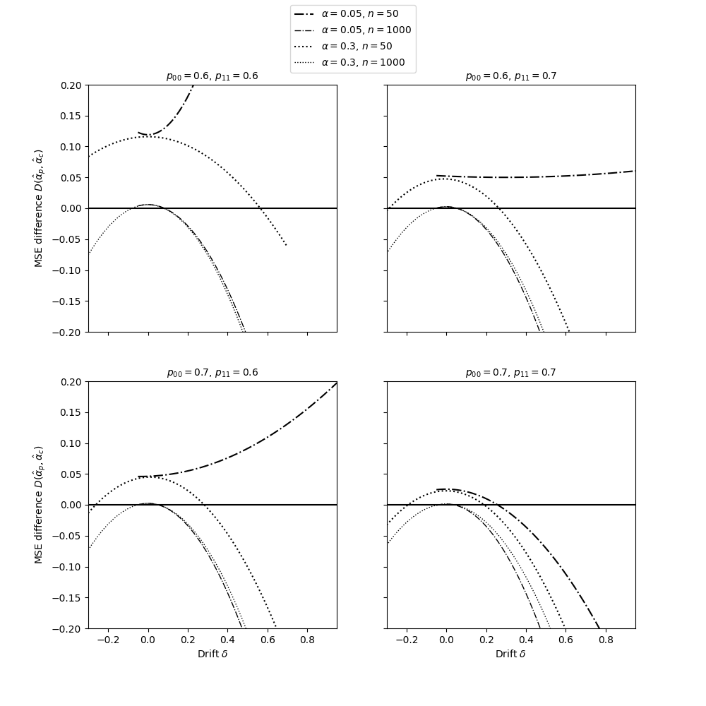
We start plotting $T/(\beta(1-\beta))$, the absolute value of the slope of the bias of the calibration estimator, as a function of the classification probabilities for different values of $\alpha$, i.e., the base rate in the test set. For visualisation purposes, we restrict the function to $p_{00}=p_{11}$, parameterised by $p$. The results are depicted in Figure 1, including the theoretical lower bound stated in Theorem 2. The slope of the bias as a function of $p$ is decreasing from $1$ at $p=0.5$ to $0$ at $p=1$. The smaller the value of $\alpha$, the later the function drops to 0. The reason is that the drift $\delta$ is defined as an absolute number and therefore it is relatively larger for smaller values of $\alpha$. From this observation we may conclude that the impact of (an absolute) drift $\delta$ on the bias of $\hat{\alpha}_{c}$ increases if $\alpha$ is further away from $0.5$, i.e., if the so-called class imbalance increases.

Subsequently, we investigate the difference $D(\hat{\alpha}_{p},\hat{\alpha}_{c})\coloneqq MSE(\hat{\alpha}_{p})-MSE(\hat{\alpha}_{c})$ between the mean squared error of the misclassification estimator and that of the calibration estimator. The value of $D(\hat{\alpha}_{p},\hat{\alpha}_{c})$ as a function of $\delta$ is depicted in Figure 2 for each possible combination of $\alpha\in\{0.05,0.3\}$, $n\in\{50,1000\}$ and $p_{00},p_{11}\in\{0.6,0.7\}$. Note that the drift $\delta$ ranges from $-\alpha$ to $1-\alpha$, because $\alpha^{\prime}=\alpha+\delta$ must lie between 0 and 1. We report the following four observations. First, the difference is positive if $\delta=0$ in any of the line plots, which corresponds to the main conclusion drawn by Kloos et al. 2020. Second, when $n$ is sufficiently large (thin lines), the difference between the line plots are small. The reason is that the contribution of the variance terms is negligible compared to that of the squared bias of $\hat{\alpha}_{c}$, which does not depend on $n$ (see Theorem 1). Third, for highly imbalanced datasets combined with small test sets, i.e., $\alpha$ close to $0$ and $n$ small (thick dash-dotted lines), the variance of $\hat{\alpha}_{p}$ dominates if either $p_{00}$ is close to $0.5$ or $p_{11}$ is close to $0.5$. As a result, the calibration estimator has lowest mean squared error, independent of the magnitude of the drift $\delta$. Fourth, if the class distribution is relatively balanced (dotted lines), the difference $D(\hat{\alpha}_{p},\hat{\alpha}_{c})$ will become negative if $\delta$ increases, but the intersection moves farther away from $\delta=0$ as $n$ decreases.

Finally, we compute, numerically, the unique positive value of $\delta$ (if it exists) at which the mean squared error of the misclassification and calibration estimator are identical. That is, we collect and reorganise the points of intersection $D(\hat{\alpha}_{p},\hat{\alpha}_{c})=0$ as discussed in Subsection 3.2. We view $D(\hat{\alpha}_{p},\hat{\alpha}_{c})$ as a map from $\mathbb{R}^{3}$ to $\mathbb{R}$ by fixing $\alpha$ and $n$ and using $\delta$, $p_{00}$ and $p_{11}$ as variables. Then, we plot the line within the two-dimensional surface $D(\hat{\alpha}_{p},\hat{\alpha}_{c})=0$ where $p_{00}=p_{11}$, resulting in Figure 3. Interestingly, the result is a decreasing function of $p$. At first, the result might seem to contradict the result obtained in the first analysis, cf. Figure 1. There, the absolute slope of the bias as function of $\delta$ decreases with increasing $p$. Hence, the mean squared error of $\hat{\alpha}_{c}$ increases more slowly as a function of $\delta$ with increasing $p$. However, the result in Figure 3 follows from the fact that the difference in variance between $\hat{\alpha}_{c}$ and $\hat{\alpha}_{p}$ rapidly decreases as $p$ increases.

We stress that the lines in Figure 3 can be interpreted as decision boundaries. Each statistical indicator that is based on a classification algorithm plots somewhere in the $(p,\delta)$-plane depicted in Figure 3. Our experimental result then reads as follows. If the plot of the indicator in the $(p,\delta)$-plane ends up above the decision boundary (which depends on $\alpha$ and $n$), then the misclassification estimator should be preferred over the calibration estimator to reduce misclassification bias. Otherwise, the calibration estimator should be preferred over the misclassification estimator. Moreover, in practice one should always compute the (estimated) bias and variance of the applied estimator, for they might still be high, e.g., when $n$ and $p$ are small and $\delta$ is large.

As a final remark, we indicate that these results hold if only the misclassification estimator and calibration estimator are considered. Admittedly, there may exist other estimators that might reduce misclassification bias even further.

References

- Beck et al. (2018) M. Beck, F. Dumpert, and J. Feuerhake. Machine learning in official statistics. arXiv:1812.10422, 2018.
- Bross (1954) I.D.J. Bross. Misclassification in 2 2 tables. Biometrics, 10(4):478–486, 1954. doi: 10.2307/3001619.
- Buelens et al. (2016) B. Buelens, P.-P. de Wolf, and C. Zeelenberg. Model based estimation at Statistics Netherlands. In European Conference on Quality in Official Statistics, Madrid, 2016. URL https://www.ine.es/q2016/docs/q2016Final00196.pdf.
- Buonaccorsi (2010) J.P. Buonaccorsi. Measurement Error: Models, Methods, and Applications. Chapman & Hall/CRC, Boca Raton, Florida, 2010. ISBN 9781420066562.
- Curier et al. (2018) R.L. Curier, T.J.A. De Jong, K. Strauch, K. Cramer, N. Rosenski, C. Schartner, M. Debusschere, H. Ziemons, D. Iren, and S. Bromuri. Monitoring spatial sustainable development: Semi-automated analysis of satellite and aerial images for energy transition and sustainability indicators. arXiv:1810.04881, 2018.
- De Broe et al. (2020) S.M.M.G. De Broe, P. Struijs, P.J.H. Daas, A. van Delden, J. Burger, J.A. van den Brakel, K.O. ten Bosch, C. Zeelenberg, and W.F.H. Ypma. Updating the paradigm of official statistics. CBDS Working Paper 02-20, Statistics Netherlands, The Hague/Heerlen, 2020.
- European Commission (2009) European Commission. Regulation of European Statistics. https://eur-lex.europa.eu/legal-content/EN/ALL/?uri=CELEX%3A32009R0223, 2009. Accessed December, 2020.
- Eurostat (2017) Eurostat. European Statistics Code of Practice. https://ec.europa.eu/eurostat/web/products-catalogues/-/KS-02-18-142, 2017. Accessed December, 2020.
- Forman (2005) G Forman. Counting positives accurately despite inaccurate classification. In J. Gama, R. Camacho, P.B. Brazdil, A.M. Jorge, and L. Torgo, editors, Machine Learning: ECML 2005, Lecture Notes in Computer Science, pages 564–575, Berlin, Heidelberg, 2005. Springer. doi: 10.1007/11564096˙55.
- Gama et al. (2014) J. Gama, I. Žliobaitė, A. Bifet, M. Pechenizkiy, and A. Bouchachia. A survey on concept drift adaptation. ACM Computing Surveys, 46(4):1–37, 2014. doi: 10.1145/2523813.
- Goldenberg and Webb (2019) I. Goldenberg and G.I. Webb. Survey of distance measures for quantifying concept drift and shift in numeric data. Knowledge and Information Systems, 60(2):591–615, 2019. doi: 10.1007/s10115-018-1257-z.
- González et al. (2017) P. González, A. Castaño, N.V. Chawla, and J.J. Del Coz. A review on quantification learning. ACM Computing Surveys, 50(5):74:1–74:40, 2017. doi: 10.1145/3117807.
- Helmbold and Long (1994) D.P. Helmbold and P.M. Long. Tracking drifting concepts by minimizing disagreements. Machine Learning, 14(1):27–45, 1994. doi: 10.1007/BF00993161.
- Kloos et al. (2020) K. Kloos, Q. A. Meertens, S Scholtus, and J. D. Karch. Comparing correction methods to reduce misclassification bias. In L. Cao, W. A. Kosters, and J. Lijffijt, editors, BNAIC/BENELEARN 2020, pages 103–129, Leiden, 2020.
- Kuha and Skinner (1997) J. Kuha and C. J. Skinner. Categorical data analysis and misclassification. In L.E. Lyberg, P.P. Biemer, M. Collins, E.D. de Leeuw, C. Dippo, N. Schwarz, and D. Trewin, editors, Survey Measurement and Process Quality, pages 633–670. Wiley, New York, 1997. doi: 10.1002/9781118490013.
- Lu et al. (2019) J. Lu, A. Liu, F. Dong, F. Gu, J. Gama, and G. Zhang. Learning under concept drift: A review. IEEE Transactions on Knowledge and Data Engineering, 31(12):2346–2363, 2019. doi: 10.1109/TKDE.2018.2876857.
- Moreno-Torres et al. (2012) J.G. Moreno-Torres, T. Raeder, R. Alaiz-Rodríguez, N.V. Chawla, and F. Herrera. A unifying view on dataset shift in classification. Pattern Recognition, 45(1):521–530, 2012. doi: 10.1016/j.patcog.2011.06.019.
- OECD (2011) OECD. Quality Framework for OECD Statistical Activities. https://www.oecd.org/sdd/qualityframeworkforoecdstatisticalactivities.htm, 2011. Accessed December, 2020.
- Schlimmer and Granger (1986) J.C. Schlimmer and R.H. Granger. Incremental learning from noisy data. Machine Learning, 1(3):317–354, 1986. doi: 10.1007/BF00116895.
- Schwartz (1985) J.E. Schwartz. The neglected problem of measurement error in categorical data. Sociological Methods & Research, 13(4):435–466, 1985. doi: 10.1177/0049124185013004001.
- Tenenbein (1970) A. Tenenbein. A double sampling scheme for estimating from binomial data with misclassifications. Journal of the American Statistical Association, 65(331):1350–1361, 1970. doi: 10.1080/01621459.1970.10481170.
- Van Delden et al. (2016) A. Van Delden, S. Scholtus, and J. Burger. Accuracy of mixed-source statistics as affected by classification errors. Journal of Official Statistics, 32(3):619–642, 2016. doi: 10.1515/jos-2016-0032.
- Webb et al. (2016) G.I. Webb, R. Hyde, H. Cao, H.L. Nguyen, and F. Petitjean. Characterizing concept drift. Data Mining and Knowledge Discovery, 30(4):964–994, 2016. doi: 10.1007/s10618-015-0448-4.
- Widmer and Kubat (1996) G. Widmer and M. Kubat. Learning in the presence of concept drift and hidden contexts. Machine Learning, 23(1):69–101, 1996. doi: 10.1023/A:1018046501280.
Appendix A Appendix
This appendix contains the proofs of the theorems presented in the paper titled “Improving the output quality of official statistics based on machine learning algorithms”. For clarity, we will write for the estimator based on the algorithms predictions . In addition to the assumptions described in Section 2, we make two more technical assumptions, namely that is independent of both the and the . It follows that and are uncorrelated and that