Native multiqubit Toffoli gates on ion trap quantum computers

In this work, we choose to be concrete and focus on a specific ion-trap system, as “the devil is often in the details” for these systems. We choose to work with the ¹⁷¹Yb⁺ ion because it is commonly used in many different quantum systems; it is used in ionQ quantum computers [12] and Honeywell quantum computers [6], while calcium is used in the shuttling quantum computers in Mainz [5]. Of course, while the details change for other ions, the general methodology is similar for other systems and it would be too much to try to describe all possible ions here. We follow closely the description given in Ref. [13].

One of the advantages of ion-trap systems is that they work with nearly ideal qubits given by atoms that are employed in atomic clocks—these systems are both well-studied and understood, but they also have coherences for the qubit states that last essentially as long as is needed for any quantum computation. Of course these systems still have significant decoherence, which arises from other mechanisms.

It is common then to use the hyperfine clock states of the ions as the pseudospin states of the quantum computer (these states often have zero total $z$-component of angular momentum, which makes them insensitive to stray magnetic fields, to first-order). The two hyperfine energy levels are the spin up (computational zero) and spin down (computational one) states of the qubit; these states are separated in energy to make it easier to address and measure them. The Hamiltonian that describes the energies of these two levels for an $N$-qubit ion-trap system is then given by

where $i$ refers to the different ion sites and $\hbar\omega_{0}$ is the energy difference between the pseudospin states. The spins are described with Pauli matrices, so that $\hat{S}_{i}^{Z}=\frac{\hbar}{2}\sigma_{i}^{Z}$. In the ¹⁷¹Yb⁺ system, we use the hyperfine clock states with total (nuclear and electronic) $z$-component of angular momentum equal to zero, given by the $\ket{F{=}0,m_{F}{=}0}$ and $\ket{F{=}1,m_{F}{=}0}$ states. The frequency difference between the energy levels is a well-known function of the magnetic field and is given by $\omega_{0}\approx 12.6$ GHz.

Because the ions are trapped in space (typically at the zeros of the effective electromagnetic pseudopotenial of the system), they also have vibrational motion relative to these equilibrium positions (we ignore the micromotion in this work). The phonon Hamiltonian that describes these vibrational modes is expanded in terms of the normal modes of the motion (determined by a simple classical analysis for the pseudopotential) [14, 15]

where $\nu$ is the index of normal mode and $\alpha$ denotes the spatial direction ($x$, $y$, or $z$). Our notation uses $x,y,z$ to represent the spatial directions of the trap and $X,Y,Z$ to indicate the pseudospin directions. The spatial motion separates into longitudinal ($z$) and transverse ($x$ and $y$) oscillations. The longitudinal modes are lower in energy than the transverse modes, and one usually works with the transverse modes in an ion trap (where the center-of-mass normal mode is the highest-energy normal mode). Often the trap has some asymmetry in the transverse direction, so the transverse mode frequencies may not always be degenerate as one would find in a perfect trap, but we ignore this small effect here. Using the raising and lowering operators of the normal modes, we find that the $\alpha^{th}$ spatial component of the position of $i^{th}$ ion is given by $\delta\hat{\textbf{R}}_{i}^{\alpha}=\sum_{\nu}b_{i}^{\alpha\nu}\sqrt{\frac{\hbar}{2m\omega_{\alpha\nu}}}\left[a_{\alpha\nu}+a_{\alpha\nu}^{\dagger}\right]$ where $b_{i}^{\alpha\nu}$ is the $\nu^{th}$ normal mode at the $i^{th}$ ion site and in the $\alpha$ direction.

In the Yb system, one addresses the ions via a spin-dependent force that is implemented with two laser beams detuned from a Raman transition to a third higher-energy atomic state. By detuning away from the precise transition, one can reduce spontaneous emission effects and continuously drive the qubit as if it is being acted on by a Pauli $X$ operator, which flips the spin from up to down (we will drop calling these clock states pseudospins from now on). A typical experimental implementation uses both red and blue detuned lasers. The effective Hamiltonian for the time-evolution is constructed by first going to the interaction representation with respect to the qubit Hamiltonian in Eq. (1), using the rotating-wave approximation and keeping only the “slow” terms, expanding the wavevector dependence in the Lamb-Dicke limit, keeping only the red and blue sideband transitions, and adjusting the phases of the laser beams to an appropriate phase lock (for further details, see Ref. [13]). The net effect, is a laser-ion Hamiltonian which drives the spin-flip transition between the qubits and is given by

where $\Omega_{i}$ is the effective Rabi frequency at the $i^{th}$ ion site and $\mu>0$ is detuning of the laser (also called the beatnote frequency, the phonons are driven to the blue of the transverse center-of-mass mode). Note that in this derivation we dropped a fast oscillating and low amplitude term driven by the carrier transitions.

In addition, we also engineer an additional uniform magnetic field (Zeeman) term by applying two lasers with frequencies separated by $\omega_{0}$. The phases of the lasers are locked to be out of phase by precisely $\pi$, to get rid of the red and blue sidebands. A second phase can then be adjusted to determine the direction of the effective magnetic field, while an acoustic-optical modulator is employed to adjust the amplitude of the field as desired. This Hamiltonian term is then

where we use a nonstandard, but common, notation for the sign of the field-spin coupling. Finally, because we went into the interaction picture with respect to the initial qubit Hamiltonian, the final Hamiltonian for the dynamics of the system is $\hat{\mathcal{H}}(t)=\hat{\mathcal{H}}_{ph}+\hat{\mathcal{H}}_{LI}(t)+\hat{\mathcal{H}}_{B}(t).$ Note that all time dependence with respect to $\hat{\mathcal{H}}_{0}$ has already been incorporated here, so we do not add additional $e^{\pm i\omega_{0}t}$ dependence to the $X$ or $Y$ Pauli spin operators. Our dynamics will now be determined by $\hat{\mathcal{H}}(t)$.

The time evolution of our system is found from the time-evolution operator. Motivated by the interaction picture, we will develop the time evolution in a hierarchical fashion by factorizing the time-evolution operator in steps. First, we develop the time evolution in the interaction picture with respect to the time-independent piece $\hat{\mathcal{H}}_{ph}$. This extracts the factor $\exp(-i\hat{\mathcal{H}}_{ph}t/\hbar)$ to the left, so that

with $\hat{U}_{I}(t)$ the standard interaction-picture time-evolution operator with respect to the phonon Hamiltonian. The interaction-picture time-evolution operator satisfies the following equation of motion

because the magnetic field Hamiltonian commutes with the phonon Hamiltonian. Evaluating the Hadamard lemma on the laser-ion Hamiltonian simply changes the vibrational raising and lowering operators into the interaction picture operators, given by $a_{\alpha\nu}^{I}(t)=a_{\alpha\nu}e^{-i\omega_{\alpha\nu}t}$ and $a_{\alpha\nu}^{\dagger I}(t)=a_{\alpha\nu}^{\dagger}e^{i\omega_{\alpha\nu}t}$. We denote this interaction-picture laser-ion Hamiltonian by $\hat{\mathcal{H}}_{LI}^{I}(t)$.

Now, we can perform a second factorization by following the methodology used in Landau and Lifshitz [16] and in Gottfried [17] for the driven harmonic oscillator. We define an operator $\hat{W}_{I}(t)=\int_{0}^{t}dt^{\prime}\hat{\mathcal{H}}_{LI}^{I}(t^{\prime})$ that has no time ordering to it. Note that $\frac{d}{dt}\hat{W}_{I}(t)=\hat{\mathcal{H}}_{LI}^{I}(t)$. Using this operator we can factorize the unitary operator $\hat{U}_{I}$ as $\hat{U}_{I}(t)=e^{-\frac{i}{\hbar}\hat{W}_{I}(t)}\hat{U}_{II}(t)$. The equation of motion for $\hat{U}_{II}(t)$ becomes

The Hadamard lemma can be evaluated explicitly for two of the three terms because the commutator of the laser-ion Hamiltonian (in the interaction picture) with itself at two different times produces an operator proportional to $\sigma^{X}$, which commutes with the laser-ion Hamiltonian. Details are given in Ref. [13]. We have

this last term is an infinite series that typically does not terminate. For a vanishing transverse magnetic field, given by $B_{Y}(t)=B_{Z}(t)=0$, Eq. (10) simplifies to the Zeeman Hamiltonian of Eq. (4) even in the interaction picture. In such a case, our interaction picture Hamiltonian reduces to a simple spin Hamiltonian $\hat{\mathcal{H}}_{s}(t)=\frac{i}{2\hbar}[\hat{W}_{I}(t),\hat{\mathcal{H}}_{LI}^{I}(t)]+\hat{\mathcal{H}}_{B}(t)$. Because the spin operators $\sigma_{i}^{X}$ in both $\hat{W}_{I}(t)$ and $\hat{\mathcal{H}}_{LI}^{I}(t)$ commute, one can easily derive that the time-dependent Ising spin Hamiltonian is given by

where we have defined $J_{ij}(t)$ as the time-dependent spin-exchange interaction and it is given by [18]

where $J_{ij}^{0}$ is the time-averaged exchange interaction and $\Delta J_{ij}(t)$ is the time-dependent part of the exchange interaction. We introduce the Lamb-Dicke parameter for the $x\nu$ mode, given by $\eta_{x\nu}=\Delta k_{x}\sqrt{\frac{\hbar}{2m\omega_{x\nu}}}$. $\Delta k_{x}$ is the $x$-component of the difference in the wavenumber for the two laser beams applied to the ion crystal. Note that the exchange interactions are generically time-dependent. Yet, most analysis of ion-trap simulators assumes the time-independent exchange interactions only. While this may sound like an extreme approximation, it actually works quite well in many cases. Part of the reason why is the phonons in the system tend to dampen the oscillations from the time-dependent spin exchange. Note further that our summation is over all $i$ and $j$. It is common to remove the (unimportant) constant terms that arise when $i=j$ and to combine the terms with unequal indices into a summation over the neighboring pairs, with an exchange constant that is twice as large. In this work, however, we continue to freely sum over both indices, but we set the diagonal terms to zero, because they are unimportant ($J_{ii}^{0}=0$).

When the transverse field is non-zero (assume here a nonzero field in the Y-direction only), we are left with a residual Hamiltonian given by $\hat{\mathcal{H}}_{res}(t)=e^{\frac{i}{\hbar}\hat{W}_{I}(t)}\hat{\mathcal{H}}_{B}(t)e^{-\frac{i}{\hbar}\hat{W}_{I}(t)}-\hat{\mathcal{H}}_{B}(t)$ after extracting the spin Hamiltonian. This residual Hamiltonian produces the residual spin-phonon interactions and is responsible for additional spin-phonon entanglement (the operator $\hat{W}_{I}(t)$ also entangles spins with phonons). But, we can still factorize $\hat{U}_{II}$ into two terms: $\hat{U}_{II}(t)=\hat{U}_{spin}(t)\hat{U}_{ent}(t)$, where the spin evolution operator is now given by

We defined $\hat{\mathcal{H}}_{spin}(t)=i[\hat{W}_{I}(t),\hat{\mathcal{H}}_{LI}^{I}(t)]/2\hbar+\hat{\mathcal{H}}_{B}(t)$ in the exponent. This factorization gives the following equation of motion for the entanglement evolution operator: $i\hbar\frac{d}{dt}U_{ent}(t)=U_{spin}^{\dagger}(t)\hat{\mathcal{H}}_{res}(t)U_{spin}(t)U_{ent}(t).$

This entanglement operator is generally quite complicated. If the time dependence of the transverse component of the magnetic field is rapid, then this time-evolution operator is close to one. In other cases, one needs to approximate it, or include it exactly, which can be done by solving for the time evolution of the combined spin and phonon systems. We will not do this here, though.

We consider the simplest example of a state selective $i$-Toffoli gate; that is, when $n=2$ (two control qubits, one target qubit), the doubly controlled $i$-Toffoli gate. For this gate, we must have three ions coupled together. Although these ions can be either in the interaction zone of a shuttling ion-trap computer or coupled via tightly focused light on a larger ion-trap quantum computer, we assume the former, so that our entire system consists of just the three ions. We also assume that the laser-spin interaction is given by the form discussed above with realistic parameters for an ion trap. Then, from Eq. (16), when all control qubits are in the up state, we have that $\Delta_{\sigma_{2},\sigma_{3}}=-4(J_{12}+J_{13})$. We detune our laser frequency close to the transverse center-of-mass phonon mode. then we obtain $J_{12}\approx J_{13}$. Note that $J$ is actually time-dependent [see Eq. (12)], but as discussed above, it is often appropriate to work with the time-averaged exchange coefficients, so, we set $B_{x}=-8J_{rms}$, where $J_{rms}=\sqrt{\sum_{i>j}|2J^{0}_{ij}|^{2}/N(N-1)}$ where $N=3$ is the total number of ions.

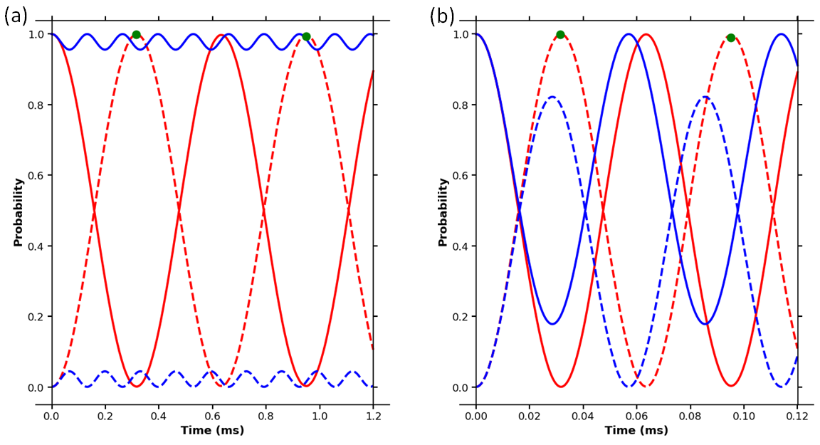
We use the following concrete parameters (all frequencies are angular frequencies) $\omega_{CM}=2\pi\times 4.63975$ MHz, Lambe-Dicke parameter $\eta=0.06$, Rabi Frequency $\Omega=2\pi\times 369.7$ KHz and a detuning of $\mu=1.0095\omega_{CM}$. The trap anisotropy is $0.2092$ for cases where the total number of ions is even and $0.1$ for cases where the total number of ions is odd (which is what we have here). Since, we have excited near the center-of-mass mode, $J_{ij}$ is approximately the same for all exchange couplings and $J_{rms}/\hbar=J^{0}/\hbar\approx 2\pi\times 926.019$ Hz. We perform simulations for two cases: (a) We ignore the time-dependence of the exchange interaction and consider the model with static exchange coupling only and (b) we use the exact form of $J(t)$ as given in Eq. (13). For both cases we take $B_{y}/\hbar=2\pi\times 75.98$ Hz, with case (a) given in Fig. (1) and case (b) in Fig. 2, respectively.

These results clearly show that the best operation occurs for the simple $\pi/2$-pulse. If we extend the simulations to longer times, we find, for example, that for the $21\pi/2$ flip the probability of success decreased to 0.8298 for time-dependent $J$ and 0.9591 for the static case. This confirms that the gate fidelity continues to drop for longer runs.

Experience with other simulations that include the full time-dependent effects of phonons showed that when those full effects were included, results were in between those of the static exchange constants and the time-dependent ones. So, to compute what is hopefully a lower bound on the fidelity, we perform the remaining calculations with time-dependent exchange coefficients (but no phonons).

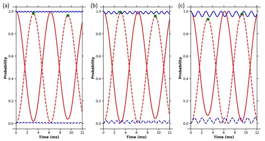
Note that the success of the gate depends on the assumption that $|\Delta-B_{x}|\gg B_{y}$ for the off-resonant spaces. We examine how the gate fidelity varies by increasing $B_{y}$. This makes the gate run faster, at the expense of reduced fidelity. This can be seen in the Fig. 3.

The probability for the target state to flip, $P_{\scriptsize\textrm{flip}}$, (which is required when control is correct) and to not flip, $P_{\scriptsize\textrm{no flip}}$, (required for all other control combinations) for different values of $B_{y}$ are listed in the Table 1. One can see that the probability to flip under the control is nearing $0.999$, but the probability to flip for other control bits, is nearly 4% in the worst case. While this is reasonable operation fidelity, the error is still somewhat high. It may require more engineering of the field, detuning, etc. to achieve better operation.

What is interesting about this approach is that the gate fidelity for the target spin to flip when the control is correct, remains essentially unchanged as $B_{y}$ is increased. The problem we encounter is that faster operation induces target spin flips in cases when the control is such that they should not flip. This will be an unacceptable gate error, as the probabilities for these “false” flips are sizable. We find a good transverse field seems to be equal to be about 1/10th of our $J_{rms}$. Note, however, that because the periods of the oscillations of the target qubit probabilities depend on the different control bit states, it may be possible to engineer a fast gate operation where we have high fidelity for all possible control qubit configurations by engineering the highest fidelity for the other control bit configurations to occur at the sames time as the $\pi/2$ pulse for the all down control. This requires a significant optimization procedure, which is not worthwhile to attempt without having the specific parameters of operation for a specific quantum computer hardware.

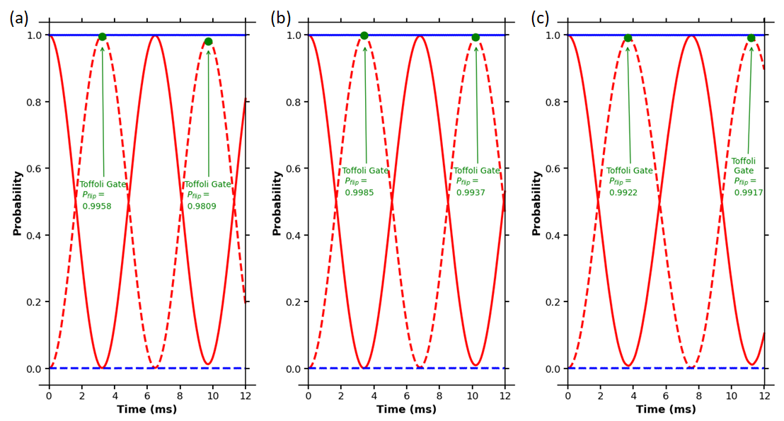
Next, we examine the effect of the detuning, as we move further from the transverse center-of-mass mode frequency (moving further into the blue). For the case where $B_{y}/\hbar=2\pi\times 75.98$ Hz, we find a degradation of the probability to not flip when the control qubits are in the wrong state, and also a degradation of the switching probability, when the control configuration is correct. These results are shown in Fig. 4.

The most likely reason for this is that the energy spacings decrease as the detuning is made larger, which creates a higher probability for an error with respect to the state of the control qubits.

Since we have proposed a method to implement an $n$-bit $i$-Toffoli gate, we also ran simulations for $n=3$, $4$ and $5$ by taking $\mu$ values such that $J_{rms}$ was nearly equal for all cases. These simulations are shown in Fig. 5. The detunings used were:

• •

  n=3: $\mu=1.00713\omega_{CM}$ $\Rightarrow$ $J_{rms}/\hbar=2\pi\times 926.307$ Hz

• •

  n=4: $\mu=1.00571\omega_{CM}$ $\Rightarrow$ $J_{rms}/\hbar=2\pi\times 925.924$ Hz

• •

  n=5: $\mu=1.00476\omega_{CM}$ $\Rightarrow$ $J_{rms}/\hbar=2\pi\times 925.876$ Hz

For these parameters, the probabilities to flip for different combinations of control qubits for n=3, 4 and 5 have been tabulated in Tables 2, 3 and 4. We see from the tables that probability to flip is large only when control is correct; i.e., $\ket{-,-,-}$.

One can see that the fidelity remains quite high for these cases. This means scaling these gates to larger $n$ values should be viable if the gate operation is short enough for efficient use in digital circuits.

A select gate is a more complicated gate than a Toffoli gate. In a select gate, the target will flip for any of the chosen controls and we have a tunable (or programmable) ability to select the control configuration (in this case by adjusting the $B_{x}$ value). The select gate is used for the sum over unitaries algorithm and is likely to have wide application in fault-tolerant quantum computers. Here, we discuss the possible applications in noisy intermediate scale quantum computers.

In the previous $i$-Toffoli gates described above, we used the center-of-mass mode because the longitudinal magnetic field lifts the degeneracy of the control state and detuning to the blue of the transverse modes produces no cross-talk with other phonon modes, since they are all lower in energy. But, when we need to also perform state inversion for control qubits in the $\ket{-,+}$ state, we find that $\Delta_{\sigma_{2},\sigma_{3}}$ is the same for both control configurations $\ket{-,+}$ and $\ket{+,-}$ in this case. Hence, we cannot invert the target qubit for each control-qubit configuration separately. To achieve a true select qubit operation, we can use detuning from the zigzag (ZZ) mode of the 3-ion system, which has $J_{12}=-2J=J_{23}$ and $J_{31}=J$ where $J$ is given by Eq. (13) with the phonon eigenvector given by $b^{ZZ}=\{0.4082,-0.8164,0.4082\}$. In this mode, if we assign site $1$ as the target ion site, we obtain four different values of $\Delta_{\sigma_{2},\sigma_{3}}$ for the four different combinations of control qubits.

We obtain $\Delta\approx 4J$, $12J$, $-12J$ and $-4J$ for control qubit state $\ket{-,-}$, $\ket{-,+}$, $\ket{+,-}$ and $\ket{+,+}$, respectively. Therefore, we can simply adjust our longitudinal magnetic field according to whichever subspace inversion is required and we have created an $i$-select gate. To use the ZZ mode, we used the fact that the transverse phonon mode frequency for zigzag mode is 0.9879 of the CM mode frequency. Thus, $\omega_{ZZ}=2\pi\times 4.58361$ MHz. We used the detuning of $0.9905\omega_{ZZ}$ (to the red of the zigzag mode) to perform the simulations of the select gate. The probabilities of flipping the target state for a given subspace are tabulated in Table 5. The action of select gate for the subspace $\Delta=12J$ has also been plotted in Fig. 6 in which we can see that the target state flips only when control qubits are in $\ket{-,+}$ state. One can see the performance here is excellent, even better than the center-of-mass tuned $i$-Toffoli gates. Of course one does have to be careful when detuning to the red of the transverse zigzag mode not to simultaneously be detuned close to the longitudinal modes, but that does not occur in this case. The longitudinal mode frequency of the zigzag mode is given by $\omega_{ZZ,L}=2.408\omega_{CM,L}$. Since, for $n=2$; i.e., a 3-ion system, our anisotropy is 0.1, we have that $\omega_{CM,L}=0.1\omega_{CM}$ which implies that $\omega_{ZZ,L}=0.2408\omega_{CM}$. This is far from the red-detuned transverse zigzag mode at $0.9879\omega_{CM}$. This means we are unlikely to excite longitudinal modes when we detune to the red of the transverse zig-zag mode.

References

- [1] Rasmussen S E, Groenland K, Gerritsma R, Schoutens K and Zinner N T 2020 Phys Rev A 101 022308
- [2] Mølmer K and Sørensen A 1999 Phys Rev Lett 82 1835
- [3] Wilson A C, Colombe Y, Brown K R, Knill E, Leibfried D and Wineland D J 2014 Nature 512 57
- [4] Mielenz M, Kalis H, Wittemer M, Hakelberg F, Warring U, Schmied R, Blain M, Maunz P, Moehring D L, Leibfried D and Schaetz T 2016 Nature Commun 7 11839
- [5] Kaushal V, Lekitsch B, Stahl A, Hilder J, Pijn D, Schmiegelow C, Bermudez A, Müller M, Schmidt-Kaler F and Poschinger U 2020 AVS Quantum Sci 2 014101
- [6] Pino J M, Dreiling J M, Figgatt C, Gaebler J P, Moses S A, Allman M S, Baldwin C H, Foss-Feig M, Hayes D, Mayer K, Ryan-Anderson C and Neyenhuis B 2020 “Demonstration of the QCCD trapped-ion quantum computer architecture” preprint arXiv:2003.01293
- [7] Berry D W, Childs A M, Cleve R, Kothari R and Somma R D 2015 Phys Rev Lett 114 090502
- [8] Childs A M and Li T 2017 Quant Inform Comp 17 901
- [9] Del Re L, Rost B, Kemper A F and Freericks J K 2020 Phys Rev B 102 125112
- [10] Tornow S, Gehrke W and Helmbrecht U 2020 “Non-Equilibrium Dynamics of a Dissipative Two-Site Hubbard Model Simulated on the IBM Quantum Computer” preprint arXiv:2011.11059
- [11] Xu L, Lee J and Freericks J K 2021 unpublished.
- [12] Grzesiak N, Blümel R, Wright K, Beck K M, Pisenti N C, Li N, Chaplin V, Amini J M, Debnath S, Chen J-S and Nam Y 2020 Nature Commun 11 2963
- [13] Wang C-C J and Freericks J K 2012 Phys Rev A 86 032329
- [14] James D F V 1998 App. Phys B 66, 181
- [15] Marquet C, Schmidt-Kaler F and James D F V 2003 App. Phys B 76 199
- [16] Landau L D and Lifshitz E M (translated by Sykes J M and Bell J S) 1977 Quantum Mechanics: Nonrelativistic Theory, third ed (Oxford: Butterworth-Heinemann)
- [17] Gottfried K 1966 Quantum Mechanics: Vol. 1 Fundamentals (New York: Benjamin)
- [18] Kim K, Chang M-S, Islam R, Korenblit S, Duan L-M and Monroe C 2009 Phys Rev Lett 103 120502
- [19] Kim K, Chang M-S, Korenblit S, Islam R, Edwards E E, Freericks J K, Lin G-D, Duan L-M and Monroe 2010 Nature 465 590
- [20] Islam R, Edwards E E, Kim K, Korenblit S, Noh C, Carmichael H, Lin G-D, Duan L-M, Wang C-C J, Freericks J K and Monroe C 2011, Nature Commun 2 377
- [21] Islam R, Senko C, Campbell W C, Korenblit S, Smith J, Lee A, Edwards E E, Wang C-C J, Freericks J K and Monroe C 2013 Science 340 583