Sensitivity of low-rank matrix recoveryThanks: PB: MPI MiS Leipzig, Inselstr. 22, 04103 Leipzig, Germany. paul.breiding@mis.mpg.de. PB has received funding from the European Research Council (ERC) under the European Union’s Horizon 2020 research and innovation programme (grant agreement No 787840) and from the Deutsche Forschungsgemeinschaft (DFG) – Projektnummer 445466444. Thanks: NV: KU Leuven, Department of Computer Science, Celestijnenlaan 200A, B-3001 Leuven, Belgium; Leuven.AI, KU Leuven Institute for AI, B-3000 Leuven, Belgium, nick.vannieuwenhoven@kuleuven.be. Supported by a Postdoctoral Fellowship of the Research Foundation—Flanders (FWO) with project 12E8119N
Abstract.
We characterize the first-order sensitivity of approximately recovering a low-rank matrix from linear measurements, a standard problem in compressed sensing. A special case covered by our analysis is approximating an incomplete matrix by a low-rank matrix. This is one customary approach to build recommender systems. We give an algorithm for computing the associated condition number and demonstrate experimentally how the number of linear measurements affects it.
In addition, we study the condition number of the rank- matrix approximation problem. It measures in the Frobenius norm by how much an infinitesimal perturbation to an arbitrary input matrix is amplified in the movement of its best rank- approximation. We give an explicit formula for the condition number, which shows that it does depend on the relative singular value gap between the th and th singular values of the input matrix.
2010 Mathematics Subject Classification
15A83, 15A12, 15A23, 65F35, 53B20, 53C42, 65F221. Introduction
Compressed sensing [14, 16, 18, 20, 24] is a general methodology for recovering an unknown but structured signal from a measurement , where can be much smaller than and is a sensing operator. The goal is to recover the unknown signal using only information about the compressed signal. We consider only affine linear maps as sensing operators in this paper.
Low-rank matrix recovery is a specific instance of compressed sensing. Herein, it is assumed that the unknown signal, an matrix , (approximately) exhibits a low-rank structure of known rank . The goal is to find a rank- matrix close to the unknown matrix from the compressed sensing .
A prominent application of low-rank matrix recovery is in collaborative filtering and recommender systems. Consider the so-called Netflix problem [8] for instance. Here, the data consists of an matrix for users and movies and the th entry contains the rating of user for movie . Not all users have rated every movie. Thus, not all entries of the data matrix are available; it is incomplete. Filling in the missing values corresponds to predicting personalized movie ratings for each user. A common assumption is that the rating of movies by users is determined by unobserved latent factors, and that a low-rank factorization reveals these factors. This assumption was exploited by several submissions of the Netflix prize competition, including SVD++ [33], timeSVD++ [35], and the eventual winning solution [34]. Recovering these latent factors from incomplete observations is a low-rank matrix recovery problem. Indeed, if the number of known ratings is , we can arrange the entries of this incomplete matrix in a vector . The projection from matrices to incomplete matrices is then a (linear) coordinate projection .
Problems that can be solved with low-rank matrix recovery include collaborative filtering [7, 44], image inpainting [26, 32, 38], dimensionality reduction [46, 47], embedding problems [39], and multi-class learning [5, 40]. In all of these applications it is important to understand the sensitivity of the output with respect to perturbations in the input. Eisenberg [19] summarizes this as follows:
“‘Many investigations of big data solve inverse problems […]. The sensitivity of results to uncertainties […] is crucial to determine the reliability and thus utility of results.”
For the Netflix problem this translates to the pertinent question of how sensitive the predicted ratings are to small perturbations in the known ratings (which by their nature are never truly exact). The urgency of this question is underlined by recent concerns about reproducibility [23], well-posedness [48], and sensitivity [3] in recommender system technologies. For example, [23] reported that the results of less than half of the considered conference papers could be reproduced. A priori, one potential, source of divergence in predicted ratings can be due to slight differences in the way the input data is centered, e.g., rounding to double, single, or half precision floating-point numbers. This may seem insignificant, but it is known that approximation problems can be very sensitive to changes to the input data due to ill conditioning [12]. How can we ascertain whether these small perturbations are not propagated to large proportions in the final predicted ratings in recommender systems based on low-rank matrix factorization?
In this paper, we consider foregoing question for low-rank matrix recovery in the setting where can be any affine linear map. Formally, the low-rank matrix recovery problem consists of solving the nonlinear least-squares problem
| (R) |
where is the Euclidean norm on . We assume that we are given a well posed problem instance. That is, a solution exists, is unique, and is locally continuous. We will return to discuss this assumption in Section 3. For now, it suffices to know that if , then for almost all (affine) linear maps and almost all incomplete matrices , the least-squares problem Eq. R is well posed by [11, Q&A 7].
Contributions
To answer the previous question for low-rank matrix recovery, we characterize the (first-order) sensitivity of the output, the unknown low-rank matrix , with respect to small perturbations of the input data, the compressed sensing . For this, we compute the condition number of the nonlinear least-squares problem Eq. R. We give a formal definition of this number in Section 3, but at this point it suffices to think about an asymptotically sharp bound
where denotes the Frobenius norm. Here, is the solution of Eq. R for the input , which is a small perturbation of . By asymptotically sharp we mean that the inequality is a sharp inequality in the limit as . We stress that the foregoing bound holds irrespective of the specific algorithm that is employed to obtain the low-rank matrix . It is an intrinsic property of the low-rank matrix recovery problem, a measure of its numerical hardness [9, 13].
Our first main contribution is a numerical linear algebra algorithm for computing the condition number of low-rank matrix recovery. This algorithm is presented in Section 7. We show in Proposition 3 below that for certain structured sensing operators, including coordinate projections, the computational complexity of the algorithm is , where is the problem size11 1 The problem size is defined here as the dimension of the optimization domain in Eq. R. It will be stated formally in Section 3. and , where the oversampling rate is typically a small constant (up to a factor , this is the same complexity as one step of a standard (Riemannian) Newton method [1, 10] for solving optimization problem Eq. R). We apply the algorithm in Section 8 to small-scale matrix recovery problems to assess the impact of oversampling () on the condition number.
Our second contribution is an explicit formula of the condition number for the special case of low-rank approximation. Here, the input data is and the problem is approximating with a matrix of low rank , i.e., solving
| (A) |
where the norm is the Frobenius norm. This problem is the special case of Eq. R when is the identity map. The usual approach for solving the low-rank approximation problem is by computing a compact singular value decomposition (SVD) with . Then, a solution of Eq. A is given by the truncated SVD . We denote the condition number in this case by . Our second main result, Theorem 2, characterizes the condition number of low-rank approximation of :
| (1) |
The sensitivity of approximating with the low-matrix thus depends on the singular value gap between and of . The input is ill-posed, if .
The last statement might seem contradictory to some literature, like [17], that might be interpreted as suggesting that “low-rank matrix approximations do not need a singular value gap” to have a small condition number. An informal example makes it clear, however, that if the recovered low-rank matrix is of interest, rather than the approximation error, then a singular value gap is required for a meaningful interpretation. For the example we denote by the two standard basis vectors and take . The best rank- approximation of is
and we have . Therefore, a large deviation of may be expected when perturbing . For example, perturbing by , results in the matrix . The best rank- approximation of is
Hence, a unit-order change results between and from a perturbation of size , as could have been anticipated from . Another more formal example is given in Example 1 in Section 5 below.
Outline
The outline of this paper is as follows. In the next section, we compare and contrast the perhaps surprising result for low-rank approximation to existing insights from the literature. Thereafter, Section 3 formally states the main results and assumptions of our study. Section 4 investigates the Hessian of the objective function from Eq. A, which provides a crucial contribution to the condition numbers of both problems Eqs. R and A. Armed with insights about the Hessian, we characterize the condition number of Eq. A in Section 5. The condition number of Eq. R is analyzed in Section 6; in this case, we are unfortunately not able to derive a closed expression. For this reason, Section 7 presents a numerical algorithm for computing it. Numerical experiments with both low-rank approximation and recovery are featured in Section 8.
Acknowledgements
We thank Sebastian Krämer for valuable feedback that led to several improvements in the presentation of our results. In particular, formulating Example 1 by formalizing the introductory example was suggested by him.
2. Comparison to prior results
In the literature we did not find results on the sensitivity of low-rank matrix recovery. However, for the special case of low-rank approximation there are several. Some of them might seem to contradict our result, while the final one corroborates it. For this reason, we carefully discuss the prior literature.
2.1. Drineas and Ipsen’s no-gap result
Drineas and Ipsen’s article [17] is titled “Low-rank matrix approximation do not need a singular value gap.” At first sight, this seems to contradict our results, but on closer inspection the paradox quickly disappears. Dirineas and Ipsen study error bounds for the approximation error of a low-rank approximation, as measured by the Schatten -norm of the residual , where is the matrix to approximate and projects onto the orthogonal complement of a fixed -dimensional subspace . That is, they derive error bounds for as either the fixed subspace or the matrix is perturbed in [17, Theorem 1] and [17, Theorem 2], respectively. For example, when perturbing , [17, Theorem 2] states that
Our results, on the other hand, describe what happens to the best rank- approximation of as it is perturbed. That is, using terminology closer to [17], we show that
where projects to the best rank- approximation.22 2 Equivalently, but closer to [17] in formulation, it projects the column space of to , the -dimensional subspace of left singular vectors associated to the largest singular values. Note that in our result both and the projector are perturbed as varies with .
2.2. An error bound of Hackbusch
Next, we discuss the result from [27] by Hackbusch. For this we let and we denote by a perturbation of . If is the best rank- approximation of and if is any other rank- matrix, then Theorem 4.5 in [27] asserts that
| (2) |
where is a constant that does not depend on the input data.
The main rationale for this bound is that could be a cheap approximation of the rank- truncated SVD, e.g., obtained from randomized methods [28] or adaptive cross approximation [6]. The bound states that if the approximation is , then deviates from by at most times . The latter can be computed from the data, so the quality of the computation can be assessed.
The fact that Eq. 2 involves a constant upper bound seems contradictory to Eq. 1. However, our result states that for sufficiently small we have
| (3) |
where is a best rank- approximation of , and are the th and th singular values of . This means that a small perturbation of the input is amplified in the output by the condition number in the worst case. If , this factor is huge.
Assume that is the true matrix we want to compute a rank- approximation of and that is a perturbation of , e.g., due to roundoff or measurement errors. In this case, the bound Eq. 2 does not tell the whole story and could be complemented with Eq. 1. Indeed, even if we can approximate closely by so that is small, the matrix can still be far from the best rank- approximation of the true matrix . Combining Hackbusch’s result with Eq. 1 yields
The first term of the final bound follows from Euclidean geometry, while the second term is the effect of curvature of the manifold of rank- matrices.
2.3. First-order perturbations of the SVD by Hua and Sarkar
The earliest result on the sensitivity of the best low-rank approximation to a matrix we could locate in the literature is by Hua and Sarkar [31]. They show that “the first-order perturbations in the SVD truncated matrices […] can be simply expressed in terms of the perturbations in the original data matrices” and they conclude from their analysis that “the SVD truncations do not affect the first order perturbations”. This also seems to contradict Eq. 1, where we show that a best rank- approximation can change by (much) more than the norm of the perturbation.
The paradox disappears when we take into account that Hua and Sarkar assume that the input is itself a rank- matrix. Thus, the th singular value of is and so, by Eq. 1, we have, once more, , which is fully consistent with their result.
2.4. Perturbation expansions of Vu, Chunikhina, and Raich
The main result of Vu, Chunikhina, and Raich [49, Theorem 1] turns Feppon and Lermusiaux’s analysis [22] into a rigorous perturbation bound for the best rank- approximation for arbitrary input matrices. We also use Feppon and Lermusiaux’s work in Sections 5 and 6. Consequently, the effect of curvature pops up in [49, Theorem 1], consistent with Eq. 1. Nevertheless, we think our first-order error bound
where is a perturbation of and and are the best rank- approximations of and respectively, is more succinct than the bound in [49, Theorem 1]. In addition, our analysis extends to the low-rank matrix recovery problem.
3. Statement of the main results
As in the introduction we consider an affine linear map
| (S) |
which is called the sensing operator. Let
be the set of matrices of rank equal to . It is a smooth embedded submanifold of of dimension [30]. This implies that the set is equipped with a topology and smoothness structure that is inherited from the ambient space . This enables a vast generalization of calculus on such domains [37]. Precisely this smooth structure will make it much easier to compute the desired condition numbers. The set of sensed matrices will be denoted by
We also define the set of matrices of rank bounded by :
It is both the Euclidean closure of and a real algebraic variety in , defined by the vanishing of -minors [29].
The goal of this paper is to determine the first-order sensitivity of Eq. R. The input to this problem is a compressed sensing , while the output is necessarily restricted to be a rank- matrix. The first complication one encounters is that there can be no or several solutions for an input . A priori we should expect to deal with a set-valued solution map The condition number of this map can be analyzed with the general techniques we introduced in [12]. In low-rank recovery, however, the geometry of the problem is more well-behaved than the general case. This allows for a clearer presentation that eliminates the intricacy of solution manifolds in [12]. We explain this next.
The geometry of our setting is depicted in Fig. 1. It illustrates that Eq. R decouples into two subproblems:
- (i)
minimizing the distance from to , and
- (ii)
inverting the map .
Fortunately, under a mild assumption, is a differentiable function almost everywhere in the precise sense of Proposition 1 below. This assumption is the following.
Assumption 1.
We assume that can be generically identified.
Being generically identifiable means that there is a Zariski open algebraic subvariety , such that for all . Q&A 7 in [11] shows that almost all have this property if .
The next result is [11, Q&A 12].
Proposition 1.
Under 1 there exist smooth embedded submanifolds and , which are both dense in their supsets, such that
is a global diffeomorphism.
A global diffeomorphism is a smooth bijective map between manifolds whose inverse map is smooth.
For minimizing the distance from to the input we consider the following open subset of the input space :
where is (the Euclidean closure of) the set of points for which does not have a unique solution (because it has multiple or no solutions). Note that we have replaced by the submanifold here. Since is an embedded33 3 This means that its smooth structure is compatible with the smooth structure on . submanifold of , the existence of a tubular neighborhood [37] of , an open neighborhood containing in , guarantees that contains at least this open subset.44 4 Erdös’s result [21] implies that the set of points which have several infima of the distance function to is of Lebesgue measure zero. However, may not be closed, and so there can be points with no minimizer on . The set of such points can even be full-dimensional. Think of a cusp with the node removed. Recently, explicit examples of nonclosedness were presented in [48] in the context of matrix completion. On we can define , the projection onto .
In summary, the foregoing closer look at the geometry of problem Eq. R allows us to arrive at a recovery map . This is the map
| (4) |
It is a smooth (uni-valued) map!
With the foregoing concessions (1, open dense submanifolds and , removing from the domain) we can apply Rice’s [45] classic definition of the condition number of a map for :
| (5) |
where is the recovered rank- matrix. If is outside the locus, where we can obtain the recovery map (5), we define .
Remark 1.
Note that Eqs. 4 and 5 allow us to study the condition number of the global minimizer of Eq. 4. By considering the graph of , we see that the results of [12] also apply in their general form. This means that the analysis in this paper also covers local minima and critical points with as in [12]. Nevertheless, for concreteness we focus on (local) minima, because they are the main interest in applications.
3.1. Low-rank matrix recovery
The condition number of (well-posed) low-rank matrix recovery in Eq. 4 at with output can be obtained from Theorem 7.3 in [12]:
| (C) |
Herein, is the spectral norm relative to the Frobenius norms on and the Euclidean norm , is the derivative of , and is the Riemannian Hessian of the squared distance function at the point . This Riemannian Hessian generalizes the classic Euclidean Hessian and contains the second derivatives of on ; it is discussed in Section 4.
As one can see from Fig. 1 and also from the formula Eq. C, the condition number is determined by two parts:
- (i)
the sensitivity of the recovery map , and
- (ii)
the curvature of the manifold of sensed rank- matrices at .
The effect of curvature on condition is depicted in Fig. 2. If is a center of curvature with base point of the parabola-shaped manifold, then the Riemannian Hessian is not invertible. In this case we have and we call the input ill-posed. The center of curvature for is shown in Fig. 2 as the gray point in the center of the displayed circle.
3.2. Low-rank matrix approximation
We turn to the special case when is the identity map. This corresponds to the problem of approximating a matrix by a rank- matrix.
The condition number of low-rank approximation is also given by Eq. C, where is the identity and . Our main result in this setting is the following result.
Theorem 2.
Let be an SVD of with ordered singular values . Let be a rank- truncated SVD of . Then, the condition number of finding a best rank- approximation at is
or if .
We prove this theorem in Section 5 below. Note that if and only if .
4. The Riemannian Hessian of the distance function
The Riemannian Hessian [36, 15, 43] generalizes the classic Hessian matrix from multivariate functions to maps on manifolds. We focus on the Riemannian Hessian of the distance function from to the smoothly embedded submanifold . This manifold is equipped with the Riemannian metric inherited from the Euclidean space . That is, every tangent space is equipped with the inner product , where are viewed as vectors in .
The goal of this section is not to provide a rigorous derivation of the Riemannian Hessian in general, but rather present an accessible account for submanifolds of Euclidean space that highlights its connection to classic differential-geometric objects like the second fundamental form and Weingarten map, which will be used in the technical results. An alternative accessible account can be found in [10, Chapter 5].
Ignoring the manifold structure for a moment, in classic multivariate analysis the Hessian of at would be
| (E) | ||||
In the classic setting, is a vector in which bears no particular relationship to . Hence, in Euclidean geometry, the second term involving vanishes.
When is restricted to lie on a manifold , the interpretation of Eq. E changes substantially. The derivative of a smooth map between manifolds at is a linear map between the respective tangent spaces [37]. This means that and are elements of , which we can view in as an affine linear space attached at . Consequently, should be interpreted as the directional derivative of the tangent vector as the base point is infinitesimally moved in the direction of . Based on this interpretation, circumventing vector fields, we could define
where is an integral curve [37] realizing , i.e., is a smooth map from a neighborhood of with and .
Since can be viewed as an affine linear subspace of , we can decompose the latter as , where is the normal space of at , i.e., the orthogonal complement of . Projecting to the normal space yields a fundamental object in Riemannian geometry, the second fundamental form [36, 41, 42, 15, 43]. This is the bilinear map
| (6) |
If we contract the output of this map with a normal vector , we obtain the so-called Weingarten map or shape operator, another classic and well-studied object in Riemannian geometry [36, 41, 42, 15, 43]:
This Weingarten map is a self-adjoint operator .
At a critical point , it follows that we can interpret Eq. E in terms of classic, well-studied objects in Riemannian geometry, namely as the following linear endomorphism on :
| (H) |
where is the identity on and is viewed as linear map . The map , or its matrix representation, is called the Riemannian Hessian.55 5 For arbitrary , the Riemannian Hessian is also defined by Eq. H for [43].
4.1. Principal curvatures
The Riemannian Hessian of contains geometric information about the way curves inside of [43]. Let , , and . The real eigenvalues of the Weingarten map are called the principal curvatures of in the direction . They measure how much curves at in the direction . If is a principal curvature of at with associated unit-norm eigenvector , then in the plane spanned by and , the intersection of the manifold with can be locally approximated to second order at by a segment of an osculating circle with center . This circular arc passes through with derivative ; see Fig. 2.
With this additional terminology, we obtain the following observation from Eq. H.
Lemma 1.
Let . Then,
where the norm is the spectral norm and the are the principal curvatures.
4.2. The second fundamental form as a tensor
By multilinear algebra [25], we can represent the second fundamental form from Eq. 6 by a three-dimensional tensor in , where denotes the dual. This tensor is symmetric in the first two factors; see [12, equation (H)] or [43] for more details.
The dual space is identified with via the standard Euclidean inner product on because is an embedded manifold inheriting the Riemannian structure from . Let and be vectors so we can write
for some ; such an expression exists [25]. The corresponding bilinear map is then Let be a normal vector at . The contraction of with along the third factor is defined by
In the standard basis of , the tensor would be represented by the rank-one matrix , so that the foregoing equation can also be viewed naturally as a matrix. Comparing with the definition of the Weingarten map and Eq. H, we see the latter can also be expressed as
| (H’) |
5. Sensitivity of low-rank approximation
In low-rank matrix approximation the sensing operator in Eq. S is given by being the identity on and . Hence, . It follows from Eq. C that the condition number of low-rank approximation is
where is the Riemannian Hessian of at .
Let and . Since minimizes the distance function , we have , i.e., is a normal vector of at . By Lemma 1, we have
| (7) |
where are the principal curvatures of at and in direction .
The principal curvatures (of open submanifolds) of can be derived from Amelunxen and Bürgisser’s Proposition 6.3 in [4] and were also stated by Feppon and Lermusiaux [22, Theorem 24]. Let be an SVD of with the singular values sorted decreasingly, and let the corresponding truncated rank- SVD be . The principal curvatures at in the normal direction are, on the one hand,
| (8) |
and the other hand principal curvatures are equal to zero [4, 22]. We can now prove Theorem 2.
Remark 2.
In Remark 1 we mentioned that the analysis of condition numbers also carries over the critical points. The critical points of the squared distance function for are all of the form , where is a subset the indices with . It can be shown that the condition number of low-rank approximation at such a critical point is .
Theorem 2 shows that if there is a clear gap between the th and th singular value, then the best rank- approximation problem is well-conditioned. However, if then the problem is nearly ill-conditioned, by Theorem 2.
In the introduction we presented an informal example of an ill-conditioned low-rank approximation. For completeness, this example is formalized next.
Example 1.
Let be fixed and consider the matrix . The condition number at the unique best rank- approximation is Let with . Consider the perturbed matrix . Its eigendecomposition is
with
Let . The unique best rank- approximation of is then
Consequently,
where the second equality is the Taylor series expansion around . Dividing by , we find
The perturbation of size that takes to moves the best rank- approximation from to . The distance between these approximations relative to the distance between the matrices is approximately plus higher-order terms in . As was fixed and arbitrary, the low-rank approximation of can be made as ill-conditioned as wanted. Note that for the condition number tends to , which in this case is caused by the occurrence of a positive-dimensional family of best rank- approximations of .
As a final observation, note that the limit for of is precisely the square of the condition number . That is, the perturbation is exactly the worst direction of perturbation for .
6. Sensitivity of low-rank matrix recovery
We continue with our discussion of low-rank recovery. Here, is a sufficiently general sensing operator for which we assume 1 and Proposition 1 hold. The point is the input data to the recovery problem, is a sensed rank- matrix approximating , and is the recoverable rank- matrix that projects to .
Recall from Eq. C that the condition number of low-rank matrix recovery is
where is the Riemannian Hessian of the squared distance to the manifold at . This section derives a closed expression for . Unfortunately, we are unable to derive a closed expression for . Therefore, we will present a simple and efficient numerical linear algebra algorithm for evaluating in the next section.
Recall from Eq. H’ that the Riemannian Hessian can be expressed in terms of the second fundamental form. Thus, our problem reduces to computing the latter. We can rely on the following lemma, which shows how curvature transforms under affine linear diffeomorphisms. While this is considered an elementary result in differential geometry, we could not locate a suitable reference, so a proof is included in the appendix for self-containedness.
Lemma 2.
Consider Riemannian embedded submanifolds and both of dimension . Let be an affine linear map that restricts to a diffeomorphism from to . For a fixed , let be a basis of . For each let . Then, is a basis of the tangent space at , and we have
This lemma shifts our problem to computing the second fundamental form of (recoverable) rank- matrices . The latter was computed in [2, Section 4.5] and [22, Proposition 22]. In the next subsection we will evaluate the latter at an orthonormal basis, so a succinct matrix representation is obtained.
6.1. Second fundamental form of rank- matrices
Let be a compact SVD of , such that is the diagonal matrix with entries the singular values . Then, by the fact that is an open submanifold of and [30], the tangent and normal spaces to at are
| (9) |
where and are conveniently identified with their column spans, denotes the direct sum of (orthogonal) linear subspaces, and denotes the orthogonal complement of a subspace. Let the columns of be , and let be the columns of . Let be an orthonormal basis of , and one for . Then,
For brevity we define for all and . We also define the rank- matrices
Then, we have the unique decomposition . We obtain the following formula from [22, Proposition 22]:
It can be verified by direct computation that the expression simplifies to
| (10) |
Herein is the Kronecker delta. The fact that restricted to is zero is actually a priori clear from geometric considerations: the second fundamental form measures the curvature of inside of and if , there is a whole linear space contained in passing through , namely . The part of the second fundamental form arising from contravariant differentiation of the basis vectors of thus vanishes completely.
Since the form an orthonormal basis, it can be deduced from Eq. 10 that the following is the second fundamental form of at viewed as element of the tensor space :
| (11) |
see also the discussion in Section 4.2. Note that since our Riemannian metric is the standard Euclidean inner product on , dualization consists of transposition.
6.2. Second fundamental form of sensed rank- matrices
We can now compute the second fundamental form of the sensed manifold .
Let us denote . These are the images of the basis vectors of under the derivative . As before, let . We conclude from Lemmas 2 and 11 that the second fundamental for , viewed as an element of , is
| (12) |
where is the dual basis vector of ; that is, .66 6 It is customary to denote the dual basis by . This dual basis is often defined with respect to an orthonormal basis in . We chose to emphasize that taking the dual of in this way does not result in the dual basis vector . Recall from Eq. H’ that the formula for the Riemannian Hessian is , where . The second term in this formula is thus
| (13) |
As discussed in Section 4.2, this expression can be represented naturally by a matrix in . The transposition on the right-hand side originated from taking duals as can be seen as a bilinear map .
Equation Eq. 13 specifies in abstract terms the contraction of the second fundental form by . We can use this to compute the condition number . Indeed, is the spectral norm of the inverse of . Unfortunately, we were not able to determine a handy expression for the inverse of . For this reason, we explain how the condition number can be computed using standard linear algebra software in the next subsection.
7. An algorithm for computing the condition number
The spectral norm in the definition Eq. C of can be computed efficiently in coordinates if we choose orthonormal bases for respectively the codomain and domain of the operator . In such bases, the spectral norm coincides with the -norm of the coordinate matrix by classic linear algebra. The inverse of the smallest singular value of this matrix representation of is then the condition number .
7.1. Determining the dual basis
First, we express the dual basis in the standard basis of . We assume that computes the coordinates in the standard basis of . Consequently, the basis vectors are given in these coordinates by Let be the matrix formed by placing the ’s as column vectors, where .
The dual basis of , expressed in coordinates with respect to the standard basis of , is then given by the rows of the Moore–Penrose pseudoinverse of ; indeed, so the rows are the dual basis vectors.
7.2. Matrix representation of the Weingarten map
From Eq. 13, we can now conclude that the matrix of the Weingarten map relative to the standard basis of and of is
where denotes an matrix of zeros, is defined in the next paragraph, and all non-displayed entries are zero. Consequently, is a square matrix of size .
We see from Eq. 13 that the foregoing matrix is indexed by a multi-index with and . Its entries are:
| (14) |
compare this with the start of the equations that led to Eq. 11.
Remark 3.
Note that for fixed , the submatrix of formed by is a multiple of the identity. After a suitable symmetric permutation of rows and columns, we thus can write , where and . This observation can be exploited to further simplify computations with . Doing this implies a particular ordering of the basis vectors in , which needs to be respected when computing below. As the computational gains associated with this observation do not lead to an improvement of the asymptotic running time, we decided not to exploit it in the discussion below.
Consider the factorization . As the columns form a basis (recall that ), is an invertible matrix. It follows that . We can thus write
Partitioning conformally with the block structure of the middle matrix, we have
where are unspecified matrices. Consequently, the foregoing expression of can be simplified to
where symmetrizes its input.
7.3. Computing the condition number
Recall that the columns of form an orthonormal basis of . Therefore, the identity is represented with respect to the standard basis on (and its dual) as . By definition, is the change of basis matrix from to represented with respect to the orthonormal basis and the standard basis on . Putting all of this together, and using Eq. H, we find that
| (15) |
where is the identity matrix. Let us write for the matrix in the middle in Eq. 15, so that . This is a matrix representation relative to the standard orthogonal basis of and the orthonormal basis on It follows that
where is the smallest singular value of the matrix and where, as before, . We can ignore because it has orthonormal columns.
7.4. The algorithm
We can now put all components together. We assume that a rank- matrix is given (factored or not). We assume without loss of generality that . We are also given and lies (approximately) in the normal space . As before, .
The numerical algorithm we propose for the condition number proceeds as follows:
- S1.
Compute orthonormal bases and for the orthogonal complements of and respectively via a full SVD of .
- S2.
Construct the change of basis matrix as well as the matrix .
- S3.
Compute the QR decomposition .
- S4.
Ensure that is numerically orthogonal to the tangent space by computing twice.
- S5.
Construct the matrix by the formula Eq. 14 and the precomputed .
- S6.
Compute the matrix following Eq. 15, and then compute .
- S7.
Compute the smallest singular value of .
- S7.
Output .
The cost of computing the condition number with the foregoing algorithm depends on the cost of applying the linear part of the sensing operator to the basis vectors . Let us denote the maximal cost by . The cost is
where in the last step we used and . For practical sensing operators with and a small constant, this usually means the cost is dominated by the cost for computing the QR-factorization of the change-of-basis matrix .
A general sensing operator has cost . As we have , this implies the overall cost for computing the condition number would be a rather impressive . Fortunately, many sensing operator are structured. Consider, for example, the structured sensing operator
| (16) |
which is defined by the matrix , the matrix and a vector . In the foregoing, is the (columnwise) Khatri–Rao product of its arguments. The derivative of is the map . Hence, if , we see that the derivative can be applied effectively by , where is the Hadamard or elementwise product. The computational complexity is only in this case. With such a sensing operator, the condition number can be computed in operations. In conclusion, we proved the next result.
Proposition 3.
Let the sampling operator be as in Eq. 16 and . Then, the condition number where and can be computed in operations, where .
This complexity is cubic in the problem size . This means that computing the solution’s condition number is as expensive as one step of a Riemannian Newton method for solving the recovery problem.
An example of such a structured sensing operator appears in the Netflix problem from the introduction. Herein, the sensing operator selects coordinates of and the other elements are unknown. This can be expressed as in Eq. 16 by taking , and .
8. Numerical experiment
We present an experiment to study the condition number of low-rank matrix recovery. It was performed on a computer running Ubuntu 18.04.5 LTS, comprising a quad-core Intel Core i7-4770K CPU (3.5GHz clockspeed) and 32GB main memory. Our Julia implementation including experiments is available from the repository https://gitlab.kuleuven.be/u0072863/MatrixRecoverySensitivity.
We investigate the sensitivity of low-rank matrix recovery where the sensing operator is a random low-rank sensing operator. The th measurement of the sensing operator performs where and are vectors whose elements are drawn i.i.d. from a standard Gauss distribution. We investigate the influence of the number of measurements
Here, is the oversampling rate: is expected to suffice for finite recoverability; see [11, Section 3].
We also investigate the influence the relative distance of the input matrix
from the sensed input manifold . Herein, is the image under of a randomly chosen rank- matrix with and random Gaussian matrices, and is a random unit-norm normal vector at . The normal vector is chosen as follows: we sample as a random Gaussian vector in and orthogonally project onto the normal space so that .
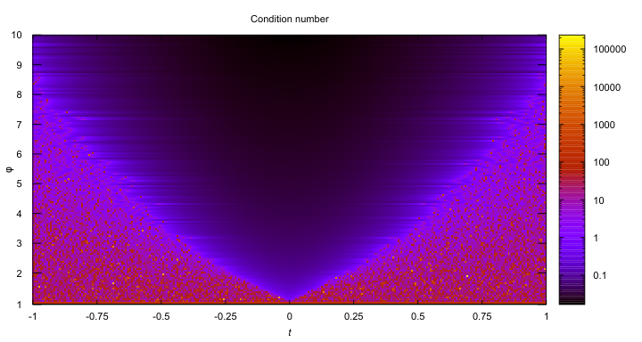
In our experiment, we took . For we took linearly spaced samples between and , and linearly spread samples between and were chosen. The corresponding number of measurements was the integer part of . Note that all vectors and are generated beforehand and we always use the first measurements for a particular . We are thus only adding measurements as is increased.
The base- logarithm of the condition number of low-rank recovery at is visualized in Fig. 3. By considering a vertical column in the figure, we can see the effect of adding additional measurements on the condition number. A phase transition can be made out in the figure. The very dark area in the figure corresponds to the cases where is a local minimizer of the distance to . In the purple–red area, on the other hand, is no longer a local minimizer and the condition numbers can be significantly higher; anywhere from around to .
The key feature Fig. 3 demonstrates is that some amount of oversampling in the measurements is necessary for very well-conditioned local minimizers, i.e., , especially when the input matrix does not lie on the manifold of sensed matrices , i.e., . In many practical applications this is true, such as in the Netflix problem, because it is only assumed that the output can be well-approximated by a low-rank matrix on . Consequently, the sensed matrix is not expected to lie on the sensed manifold either.
Appendix A Proof of Lemma 2.
We restate Lemma 2 in terms of vector fields, as required by the proof, and then we prove it.
Lemma 2 (The second fundamental form under affine linear diffeomorphisms)
Consider Riemannian embedded submanifolds and both of dimension . Let be an affine linear map that restricts to a diffeomorphism from to . For a fixed let be a local smooth frame of in the neighborhood of . For each let be the vector field on that is -related to . Then is a smooth frame on in the neighborhood of , and we have
Herein, should be viewed as an element of the tensor space by dualization relative to the Riemannian metric, and likewise for .
Proof.
Our assumption of being a diffeomorphism implies that is a smooth frame. Let , and be the integral curve of starting at (see [37, Chapter 9]). Let be the corresponding integral curve on at . Since is -related to , we have
where is the derivative of at restricted to the tangent space . On the other hand, , so that
| (17) |
The fact that the derivative of is constant is the key part in the proof. Interpreting as a smooth curve in and as a smooth curve in , we can take the usual derivatives at on both sides of Eq. 17:
Recall that . We can decompose the right hand side into tangent and normal part at , so that
Observe that that , where . Projecting both sides to the normal space of at yields
The claim follows by applying the Gauss formula for curves [36, Lemma 8.5] on both sides. ∎
References
- [1] P.-A. Absil, R. Mahony, and R. Sepulchre, Optimization Algorithms on Matrix Manifolds, Princeton University Press, 2008.
- [2] P.-A. Absil, R. Mahony, and J. Trumpf, An extrinsic look at the Riemannian Hessian, Geometric Science of Information, Lecture Notes in Computer Science, Springer, Berlin, Heidelberg, 2013.
- [3] B. Adcock and N. Dexter, The gap between theory and practice in function approximation with deep neural networks, SIAM J. Math. Data Sci. 3 (2021), 624–655.
- [4] D. Amelunxen and P. Bürgisser, Intrinsic volumes of symmetric cones and applications in convex programming, Math. Program. 149, Ser. A (2015), 105–130.
- [5] A. Argyriou, T. Evgeniou, and M. Pontil, Convex multi-task feature learning, Mach. Learn. 73 (2008), no. 3, 243–272.
- [6] M. Bebendorf and S. Rjasanow, Matrix compression for the radiation heat transfer in exhaust pipes, pp. 183–192, 2000.
- [7] R. Bell, Y. Koren, and C. Volinsky, Matrix factorization techniques for recommender systems, Computer 42 (2009), no. 8, 30–37.
- [8] J. Bennett and S. Lanning, The Netflix Prize, Proceedings of KDD Cup and Workshop, 2009.
- [9] L. Blum, F. Cucker, M. Shub, and S. Smale, Complexity and Real Computation, Springer-Verlag, New York, 1998.
- [10] N. Boumal, An Introduction to Optimization on Smooth Manifolds, Available online, 2020.
- [11] P. Breiding, F. Gesmundo, M. Michalek, and Vannieuwenhoven, Algebraic compressed sensing, arXiv:2108.13208 (2021).
- [12] P. Breiding and N. Vannieuwenhoven, The condition number of Riemannian approximation problems, SIAM J. Optim. 31 (2020), 1049–1077.
- [13] P. Bürgisser and F. Cucker, Condition: The Geometry of Numerical Algorithms, Springer, Heidelberg, 2013.
- [14] E. J. Candès, J. K. Romberg, and T. Tao, Stable signal recovery from incomplete and inaccurate measurements, Comm. Pure Appl. Math. 59 (2006), no. 8, 1207–1223.
- [15] M. do Carmo, Riemannian Geometry, Birhäuser, 1993.
- [16] D. L. Donoho, Compressed sensing, IEEE Trans. Inform. Theory 52 (2006), no. 4, 1289–1306.
- [17] P. Drineas and I.C.F. Ipsen, Low-rank matrix approximations do not need a singular value gap, SIAM J. Matrix Anal. Appl. 40 (2019), no. 1, 299–319.
- [18] M. F. Duarte and Y. C. Eldar, Structured compressed sensing: From theory to applications, IEEE Trans. Signal Process. 59 (2011), no. 9, 4053–4085.
- [19] R. Eisenberg, Reflections on Big Data and Sensitivity of Results, SIAM News 53 (2020).
- [20] Y. C. Eldar and G. Kutyniok (eds.), Compressed Sensing: Theory and Applications, Cambridge University Press, 2012.
- [21] P. Erdös, Some remarks on the measurability of certain sets, Bull. Amer. Math. Soc. 52 (1945), 107–109.
- [22] F. Feppon and P. F. J. Lermusiaux, A geometric approach to dynamical model order reduction, SIAM J. Matrix Anal. Appl. 39 (2018), 510–538.
- [23] M. Ferrari Dacrema, S. Boglio, P. Cremonesi, and D. Jannach, A troubling analysis of reproducibility and progress in recommender systems research, ACM Trans. Inform. Sys. 39 (2021), no. 20.
- [24] S. Foucart and H. Rauhut, A Mathematical Introduction to Compressive Sensing, Birkhäuser, New York, NY, 2013.
- [25] W. Greub, Multilinear Algebra, 2 ed., Springer-Verlag, 1978.
- [26] Ch. Guillemot and O. Le Meur, Image inpainting: Overview and recent advances, IEEE Signal Process. Magazine 31 (2014), 127–144.
- [27] W. Hackbusch, New estimates for the recursive low-rank truncation of block-structured matrices, Numer. Math. 132 (2016), 303–328.
- [28] N. Halko, P. G. Martinsson, and J. A. Tropp, Finding structure with randomness: Probabilistic algorithms for constructing approximate matrix decompositions, SIAM Review 53 (2011), no. 2, 217–288.
- [29] J. Harris, Algebraic Geometry, A First Course, Graduate Text in Mathematics, vol. 133, Springer-Verlag, 1992.
- [30] U. Helmke and J. B. Moore, Optimization and Dynamical Systems, Springer, 1994.
- [31] Y. Hua and T. K. Sarkar, A perturbation theorem for sensitivity analysis of SVD based algorithms, Proceedings of the 32nd Midwest Symposium on Circuits and Systems, 1989, pp. 398–401.
- [32] J.-H. Kim, J.-Y. Sim, and C.-S. Kim, Video deraining and desnowing using temporal correlation and low-rank matrix completion, IEEE Trans. Image Process. 24 (2015), 2658–2670.
- [33] Y. Koren, Factorization meets the neighborhood: A multifaceted collaborative filtering model, Proceedings of the 14th ACM SIGKDD International Conference on Knowledge Discovery and Data Mining (New York, NY, USA), KDD ’08, 2008, pp. 426–434.
- [34] by same author, The BellKor solution to the netflix grand prize, 2009.
- [35] by same author, Collaborative filtering with temporal dynamics, Proceedings of the 15th ACM SIGKDD International Conference on Knowledge Discovery and Data Mining (New York, NY, USA), KDD ’09, 2009, pp. 447–456.
- [36] J. M. Lee, Riemannian Manifolds: Introduction to Curvature, Springer-Verlag, 1997.
- [37] J. M. Lee, Introduction to Smooth Manifolds, 2 ed., Springer, New York, USA, 2013.
- [38] W. Li, L. Zhao, Z. Lin, D. Xu, and D. Lu, Non-local image inpainting using low-rank matrix completion, Comput. Graph. Forum 34 (2015), 111–122.
- [39] N. Linial, E. London, and Y. Rabinovich, The geometry of graphs and some of its algorithmic applications, Combinatorica 15 (1995), no. 2, 215–245.
- [40] G. Obozinski, B. Taskar, and M.I. Jordan, Joint covariate selection and joint subspace selection for multiple classification problems, Stat. Comput. 20 (2010), no. 2, 231–252.
- [41] B. O’Neill, Semi-Riemannian Geometry, Academic Press, 1983.
- [42] by same author, Elementary Differential Geometry, revised second edition ed., Elsevier, 2001.
- [43] P. Petersen, Riemannian Geometry, second ed., Graduate Texts in Mathematics, vol. 171, Springer, New York, 2006.
- [44] J.D.M Rennie and N. Srebro, Fast maximum margin matrix factorization for collaborative prediction, Proceedings of the International Conference of Machine Learning (2005).
- [45] J. R. Rice, A theory of condition, SIAM J. Numer. Anal. 3 (1966), no. 2, 287–310.
- [46] L.K. Saul and K.Q. Weinberger, Unsupervised learning of image manifolds by semidefinite programming, Int. J. of Computer Vision 70 (2006), no. 1, 77–90.
- [47] A. So and Y. Ye, Theory of semidefinite programming for sensor network localization, Math. Program. 109 (2007), no. 2-3, Ser. B, 367–384.
- [48] J. Tanner, A. Thompson, and S. Vary, Matrix rigidity and the ill-posedness of robust PCA and matrix completion, SIAM J. Math. Data Sci. 1 (2019), 537–554.
- [49] T. Vu, E. Chunikhina, and R. Raich, Perturbation expansions and error bounds for the truncated singular value decomposition, Linear Algebra Appl. 627 (2021), 94–139.