See pages 1 of titlepage00.pdfSee pages 1 of titlepage.pdf
Statement of Originality
I hereby certify that the work embodied in this thesis is the result of original research done by me except where otherwise stated in this thesis. The thesis work has not been submitted for a degree or professional qualification to any other university or institution. I declare that this thesis is written by myself and is free of plagiarism and of sufficient grammatical clarity to be examined. I confirm that the investigations were conducted in accord with the ethics policies and integrity standards of Nanyang Technological University and that the research data are presented honestly and without prejudice.
13/08/2020 ![[Uncaptioned image]](2103.00401v1/DhimanSignV2.PNG)
. .
Date Dhiman Bhowmick
Supervisor Declaration Statement
I have reviewed the content and presentation style of this thesis and declare it of sufficient grammatical clarity to be examined. To the best of my knowledge, the thesis is free of plagiarism and the research and writing are those of the candidate’s except as acknowledged in the Author Attribution Statement. I confirm that the investigations were conducted in accord with the ethics policies and integrity standards of Nanyang Technological University and that the research data are presented honestly and without prejudice.
13/08/2020 ![[Uncaptioned image]](2103.00401v1/PinakiSign.PNG)
. .
Date Pinaki Sengupta
Authorship Attribution Statement
This thesis contains material from two papers published in the following peer-reviewed journals.
Chapter-3 is published as D. Bhowmick and P. Sengupta. Antichiral edge states in Heisenberg ferromagnet on a honeycomb lattice. Physical Review B 101, 195133 (2020). DOI: 10.1103/PhysRevB.101.195133.
Chapter-4 is published as D. Bhowmick and P. Sengupta. Topological magnon bands in the flux state of Shastry-Sutherland lattice model. Physical Review B 101, 214403 (2020). DOI: 10.1103/PhysRevB.101.214403.
Chapter-5 is on the arXiv repository as D. Bhowmick and P. Sengupta. Weyl-triplons in . arXiv identifier: arXiv:2004.11551. (under review)
The contributions of the co-authors in all papers are as follows:
- •
I and Pinaki Sengupta provided the initial project direction.
- •
All analytical calculations and programming codes were done by me, and I performed the numerical simulations.
- •
The results were analyzed by me with the help of Professor Sengupta.
- •
I and Professor Sengupta prepared the manuscript drafts.
13/08/2020
. .
Date Dhiman Bhowmick
Abstract
The study of topological magnetic excitations have attracted widespread attention in the past few years. The wide variety of ground state phases realized in different two-dimensional magnets have emerged as versatile platforms for realizing magnetic analogues of topological phases uncovered in electronic systems over the past two decades. Dzyaloshinskii-Moriya(DM) interactions, that are ubiquitous in many quantum magnets, and has been demonstrated to induce a non-trivial topology in the magnetic excitations in many quantum magnets. In particular, signatures of DM-interaction induced topological features observed in the dispersion of magnetic excitations in the geometrically frustrated Shastry-Sutherland compound and honeycomb ferromagnet have provided the motivation behind the bulk of the research presented in this thesis. In the first chapter we introduce the background and motivation of our study. We showed that the vastly available materials with a possibility of non-zero symmetry allowed DM-interaction motivate us to study the minimal models of interacting spins related to the materials.
In the second chapter we have described the methods that is used to study the spin systems. To describe the spin excitations in the long-range ordered system and dimerized system, we use Holstein-Primakoff transformation and bond-operator formalism respectively. The Schwinger Boson mean field theory is applicable for any generic magnetic ground state and useful to study the system at high temperatures compared with Holstein-Primakoff transformation. After transforming the Hamiltonian into a quadratic bosonic Hamiltonian, it is diagonalized by using Bogoliubov-Valatin transformation. Different observables like Berry-curvature, Chern-number, Dynamical Spin structure factor etc. are calculated by using the single particle wave-function obtained from Bogoliubov-Valatin transformation. A non-zero Berry curvature is a signature of topologically protected edge states in a stripe geometry of a lattice and a systematic way of calculating edge states is also explained in the second chapter. Moreover in the second chapter the usefulness of symmetry in obtaining band degeneracies and the allowed spin-spin interaction terms are also described.
The past theoretical studies show the presence of topological magnons in honeycomb ferromagnetic models due to presence of DM-interaction on a next-nearest neighbour bonds. Recently this kind of DM-interaction is detected in the honeycomb ferromagnet . This type of DM-interaction induces chiral edge states of magnon in the system and so we named it as chiral DM-interaction. In the third chapter we show that breaking of inversion symmetry at the center of honeycomb structure gives rise to a extra DM-interaction which we named as anti-chiral DM-interaction. We studied the system by using Schwinger Boson mean field theory and Holstein-Primakoff transformation and show that when the antichiral DM-interaction dominates over the chiral DM-interaction, the direction of velocity of the edge states become in the same direction (antichiral edge states). Due to conservation of total number of spins in the system a bulk current flows in the opposite direction relative to the antichiral edge current. In this study we suggested the way to break the inversion symmetries in the materials , , (A=Ba, Cs, K, La) to achieve antichiral DM-interaction. The presence of antichiral edge states can be detected by using inelastic neutron scattering by detecting the band tilting at and points of magnon bands. Moreover we showed that spin noise spectroscopy at the edges is useful measurements to detect the presence of antichiral edge modes. Magnetic force microscopy is also a promising tool to detect the antichiral magnons at edges.
The underlying spin-Hamiltonian of the antiferromagnetic systems in the materials like rare-earth tetraborides(, R=Er,Tm) and can be described by using extended Shastry-Sutherland models. In previous theoretical studies it is shown that there is a non-collinear spin-state known as flux state exists in the Shastry-Sutherland model in presence of out of plane DM-interaction. Although the presence of perpendicular component of DM-interactions in the rare-earth materials are not known, it can be induced artificially by using circularly polarized light or using heavy-metal alloys. In the fourth chapter, we studied the magnetic excitations in the flux state on Shastry-Sutherland lattice incorporating realistic in-plane DM-interactions (using the DM-interactions present in the low symmetry crystal structure of ) by using Holstein-Primakoff transformation and showed the presence of topological magnon bands with non zero Chern-numbers in the system. We found a variety of band topological transitions and showed that each band-topological transition is associated with the logarithmic divergence in the derivative of the thermal Hall conductance. We derived a analytical expression for the temperature dependence of the derivative of thermal Hall conductivity near band topological transition point for a generic spin model. This is useful to extrapolate the energy of band touching point during the band topological phase transition by using thermal Hall effect experiment.
In the fifth chapter the spin systems related to Shatry-Sutherland lattice is described. There are three possible phases in Shastry-Sutherland model and those are (i) dimer-phase, (ii) plaquette order phase and (iii) Nèel phase. The dimer-phase material possesses two crystal symmetries; one is low symmetry phase (at low temperature) in which case both the in plane and out of plane DM-interactions are allowed; another is high symmetry phase (at high temperature) in which only the out of plane DM-interaction is allowed. We use bond operator formalism to show the existence of Weyl-triplons in low crystal symmetry structures of Shastry-Sutherland lattice. We predict that the low symmetry phase of at low temperature should contain Weyl-triplons in presence of any finite interlayer perpendicular DM-interactions and at low temperature the Weyl-triplon phenomenon is not altered in presence interlayer in-plane DM-interaction and Heisenberg interaction. There are several band topological transitions happen by changing the external magnetic field and interlayer DM-interaction (which might be varied by applying a pressure). The topological nature of Weyl triplons are confirmed by the presence of the non-zero Berry-curvature and monopole charge of Weyl-point in the bulk system. Again topological non-triviality is further confirmed by showing that at the surface of the material the Weyl-points are connected by Fermi-arc like surface states which is possible to detect by neutron scattering. Using Kubo-formula of thermal conductivity it is shown that the thermal Hall conductivity of the triplons has a quasi-linear dependence as a function of magnetic field in the Weyl-triplon region and this functional feature is absent in topologically trivial or non-trivial gapped triplon bands.
Acknowledgements
First of all, I would like to thank my research supervisor Prof. Pinaki Sengupta for his continuous support and guidance throughout my Ph.D. study on and off the field. whenever I went to his office with a problem he always welcomed me and assisted me. He has encouraged and inspired me to become an independent researcher and developed my critical thinking. I am really grateful to him as a person who introduced me the field of research. Moreover my scientific writing and presentation skills also improved due to his suggestions. I am really very thankful for being so flexible and allowing me to choose the work and project which interests me most. I am really lucky to have such fabulous supervisor.
I met many professors and lecturers in my life who inspired me and shaped my thinking through the journey from high school to masters. I have completed my secondary and higher secondary education from Barisha High School in Kolkata. I am very glad to be student under the teachers Anup Maity(Math), Brindaban Sardar(English), Arindam Mandal(Physics), Indranil Dutta (Computer Science), Prabir Roy(Biology). I have achieved my Bachelors degree in physics from Vivekananda College under Calcutta university. I am also very proud to be a student under former professor Chapal Kumar Chattopadhyay, associate professor Arivind Pan. I am really motivated by the teaching of former professor Chapal Kumar Chattopadhyay. According to him, it is easier to forget the equations in physics and the only way to remember physics is to understand the physics in your own way or language. I always have a motivation to make myself a influential physics professor like him. I pursued my masters degree in physics from Indian Institute of Technology(IIT), Kharagpur. I am very happy to be student under Professors Sugata Pratik Khastgir, Sayan Kar, Debraj Choudhury, Shivkiran B.N. Bhaktha, Ajay Kumar Singh, Somnath Bharadwaj, Maruthi Manoj Brundavanam, Samudra Roy, Samit Kumar Ray, Krishna Kumar and others. Special thanks to professor Sugata Pratik Khastgir for his advice on choosing coursework in my Master’s before pursuing a Ph.D., and thanks for his suggestion on understanding any formalism in physics through examples and thanks for his teaching in group-theory. Thanks to all other professors and teachers whom I have not mentioned in the acknowledgment, but they are equally important for my learning experience throughout my student life.
I would also like to thank Prof. Justin Song and Prof. Shengyuan Yang for being my thesis advisory committee members. I would like to acknowledge, in no particular order, the current and ex-members of our group as good friends, colleagues and well-wisher, Munir Shahzad, Ong Teng Siang Ernest, Rakesh Kumar, Nyayabanta Swain, Bobby Tan, Ho-Kin Tang. I am thankful to my friends, in no particular order, Shampy Mansha, Md Shafiqur Rahman, Bivas Mondal, Deblin Jana, Jit Sarkar, Mrinmoy Das, Bapi Dutta, Pankaj Majhi, Sourav Mitra, Rakesh Maiti for making my stay at NTU memorable and fruitful. Again I like to thank my friends Bhartendu Satywali and Subhaskar Mandal, sharing their knowledge particularly in the field of my study. In four years of staying in Singapore it was also a great experience making friends with Singaporean, again in no particular order, Ong Teng Siang Ernest, Eugene Tay, Png Kee Seng, Zhao Zhuo, Alex Lim; again thanks to them being part of my journey as a Ph.D. student in Singapore. Moreover I am thankful to Jareena being a special part of my life; taking care and supporting me through this Ph.D. journey. Finally, I would like to express my deepest appreciation to my Family- my mother Minati Bhowmick, my father Dhanu Kumar Bhowmick, my cousin Mampi Guha Majumder and my aunty Jharna Guha Majumder, for their endless support and unconditional love all the way long. I appreciate it a lot and love you all!!!
Glossary
Abbreviations
Chapter 1 Introduction
1.1 Background and Motivations
Condensed Matter physics is the branch of physics devoted to understanding the emergence of macroscopic properties of matter from (local) microscopic interactions between constituent particles and their arrangement. These can be molecules, atoms, electrons or quasi-particles such as phonons or magnons. On the theoretical front, this involves constructing microscopic Hamiltonians and solving for the emergent properties using exact or (more often) approximate analytica methods, and numerical simulations. On the experimental front, this involves measuring definitive physical properties and interpreting them in terms of microscopic modeling. Although the fundamental building block that make up all materials are atoms, different arrangements of the atoms in different materials give rise to different properties, this is known as principle of emergence. Landau [2] discovered that the key to understand different phases of the materials are related to different symmetries of the system and phase transitions are associated with change in symmetry of that system. Later Ginzburg and Landau [3] developed a general theory for phase transition based on the idea of order parameter which transforms non-trivially under phase transition or change in the symmetry. In last three decades a different picture has emerges following the discovery of integer quantum Hall effect which was experimentally detected in two-dimensional electron gas in MOSFET at low temperature and at high magnetic field [4], just after theoretical prediction of this novel phenomenon in two-dimensional material [5]. The phase transitions of different plateaus observed in the integer quantum Hall effect can not be described in the framework of Landau’s symmetry breaking theory, because in different plateau neither the symmetry of the material changes nor any local order-parameter of the system alters. Following the work of Laughlin, we know that the integer quantum Hall states arise due to the presence of the edge states present at the boundary of the system. These edge states emerges due to non-trivial topology of the bulk wave function of the system which is quantified by using Chern or Thouless– Kohmoto–Nightingale–den Nijs number [6, 7]. This topological invariant can only be changed by closing bulk energy gap of the system and that is why the bulk of the integer Hall quantum system become conducting during the transitions between two plateau regions. It was long thought that topological states are rare and it is only possible under extreme conditions. However, with the advent of spin-orbit induced topological insulators, it became clear that topological quantum states are more abundant than previously thought. Haldane’s paradigmatic model [8] showed the possibility of topological bands with non-zero Chern-numbers in the band-structure for a tight binding model of spinless particles on a honeycomb lattice with complex next-nearest-neighbor hopping. Later Kane and Mele [9] illustrated that the complex hopping term naturally emerges from spin-orbit interactions in the electron system and at the same time it was realized experimentally in the materials HgTe/CdTe semiconductor quantum wells [10, 11], in InAs/GaSb heterojunctions sandwiched by AlSb [12, 13], in BiSb alloys [14], in Bi2Se3 [15, 16], and in many other systems [17, 18]. Unlike Haldane’s model, the spin orbit induced topological electronic band systems are protected by timer-reversal symmetry i.e. in the absence of time-reversal symmetry, it is possible to adiabatically transform the spin-orbit-induced topological insulators into a topologically trivial state without closing the bulk gap. The topological invariant that correspond to these time-reversal symmetry protected topological state is -invariant and the boundary of the system manifests gap-less Helical edge modes which consists pair of counter propagating electronic states. The experimental manifestation of these Helical edge modes is the novel quantum spin Hall effect. In case of three dimensional materials, topological nodal semimetals are gapless systems which exhibits band topology even when the bulk band gap closes at certain points in the Brillouin zone. Dirac-semimetals ( [19]), Weyl-semimetals (TaAs [20, 21]), nodal-line semimetals [22, 23, 24] are the examples of gapless topological semimetals.
Band topological systems such as those mentioned above can be realized within a free electron system without any electron-electron interaction, where spin orbit coupling plays an important role to induce topology. Interactions also play an important role to generate a avenue of new kinds of topological states, like fractional topological insulators [25, 26, 27, 28], interaction induced topological insulators [29, 30, 31, 32], quantum spin-liquids [33, 34, 35], Haldane spin- chain [36, 37, 38] and so on.
A promising place to look for the interplay between interaction and spin-orbit interaction induced topological states is to study the physics of widely available magnetic ground states in different lattices. In these systems, the electron’s charge degrees of freedom are frozen due to large on-site and neighbouring site electron-electron interactions, but spin degrees of freedom of electrons remain due to the quantum fluctuations present in the system. These separated spin-degrees of freedoms are represented as bosonic quasi-particles known as spinon. At low temperature specific flavour of spinons Bose-Einstein condensate to form the magnetic ground state of the system and remaining spinonflavours constitute magnetic excitations above the magnetic ground state, which are known as spin-waves or magnons. In magnetic systems the spin-orbit coupling shows up in the form of Dzyaloshinskii-Moriya Interaction (DMI)and anisotropic interactions [39, 40]. Presence of the DMIintroduces non-trivial topology in the magnonbands. The charge neutral magnons carry information in the form of magnetic moment and being a charge neutral particle magnons do not respond to an external electric field and consequently, do not exhibit conventional Hall effect. However a temperature gradient across the topological magnon material induces transverse thermal magnon Hall conductivity. Thus the study of toplogical magnons is very important in the emerging field of magnon based spintronic devices. Transport of magnons does not produce any Joule heating effect in the device because of its’ charge neutral nature. So the magnonbased spintronic devices are very attractive with regard to low waste energy production and power consumption. For their successful engineering, it is necessary to understand the fundamental transport properties of magnons.
All of the particles electrons, phonons and magnons can cause a non-zero thermal Hall effect. The magnoninduced Thermal Hall effect was first proposed by Katsura et al. [41] in presence of interaction due to spin-chirality (order of , where is the hopping amplitude and is the onsite repulsion in Hubbard model) in the Kagome lattice. Later on Onose et al. [42] first discovered the DMIinduced magnonthermal Hall effect of the insulator , which is basically a pyrochlore lattice made of ferromagnetically ordered spins on vanadium atoms below the Curie temperature . Afterwards, several pyrochlore materials , [43] are observed to exhibit the thermal magnonHall effect phenomenon below Curie temperature. The two-dimensional projection of a pyrochlore lattice along -plane forms the geometrically frustrated kagome lattice. However topological magnonbands in collinear ground-states in a Kagome lattice have also been discovered in the material Cu(1-3,bdc) [44, 45]. Generally the Curie-temperatures of most of the magnetic materials are lower than room-temperature and even at higher temperature (less than Curie-temperature) the width of the magnonbands broden and possibly a topological phase transition can occur due to band-gap closing. So, it was thought previously that topological magnonHall effect is only possible at low temperatures, until recently the discovery of topological magnonHall-effect in Kagome ferromagnet at room temperature [46]. Kagome lattice with antiferromagnetic nearest neighbour Heisenberg interaction is a frustrated magnetic system and frustration of magnetic lattices is a key ingredient to generate non-coplanar magnetic ground states (e.g. antiferromagnetic order with a out of plane magnetic field). The non-coplanar magnetic structure produces non-zero scalar spin chirality which acts as a source of Berry-phase for magnons [47, 48]. Scalar spin chirality induced topological magnonbands are theoretically shown to be present in the -antiferromagnetic order of the frustrated kagome [49], honeycomb [50] and triangular lattices [50, 51]. It is also fascinating that several magnon-band-topological transitions occur in a non-coplanar magnetically ordered system because change in parameters are responsible for change in the scalar spin chirality resulting in a different Berry-phase of the magnons [51]. Furthermore Lu et al. [52] demonstrate that even in absence of scalar spin chirality in the antiferromagnetic systems, the topological Berry-phase of magnons can be generated via quantum fluctuations of scalar spin-chirality. Other studied frustrated lattice systems for topological magnonsystem are frustrated star-lattice [53] and Shastry Sutherland (SS)-lattice [54] with ferromagnetic ground state.

In chapter Ch. 4, we discuss the toplogical magnonband system in a non-coplanar magnetic ground state on the frustrated SS-lattice (see Fig. 1.1(a)). The rare-earth tetraborides are the material realization for frustrated SS-lattices because the antiferromagnetic Heisenberg-interactions on the dimer and axial bonds are nearly equal () [55, 56, 57]. Shahzad et al. [58] show that for a classical spin systems in , crystal-symmetry allowed perpendicular DMIon the axial bond gives rise to coplanar flux state (see Fig. 1.1(b)). If the crystal structure is such that the dimer bonds are out of plane as shown in the dimer-bonds are out of plane as shown in the figure Fig. 1.1(c), then in plane DM-interactions are symmetry allowed. In presence any in-plane DMI, the co-planar flux state become a non-coplanar canted-flux state (see Fig. 1.1(d)) and in presence of magnetic field the magnonbands in this state become topologically non-trivial. The topology of the magnonbands in the system is due to the interplay among DMI, scalar-spin chirality and quantum fluctuation of scalar spin chirality. This results in a wealth of band topological transitions with varying parameter which gives us the opportunity to study the behaviour of thermal Hall conductivity at band topological transition point. It was already known that the derivative thermal Hall conductivity shows a logarithmic divergence at the band topological transition Dirac-point [51], but here we found that the logarithmic divergence is quite universal independent of the type of band touching point. Finally we derived a simple algebraic equation for Thermal Hall conductivity as a function of temperature, which is applicable for any generic spin model and experimentally useful for determining the band-touching point during band topological transition.
On the other hand honeycomb lattice is an important lattice that supports Dirac electrons and gained much attention after the discovery of graphene by using mechanical exfoliation [59]. The magnonversion of Dirac-semimetal can also be realized in the honeycomb ferromagnets [60, 61]. Similar to the electronic Dirac-point, the magnonDirac-point in these systems are robust against magnon-magnoninteractions [62]. The Dirac-magnonis possible to gap out by breaking the inversion symmetry resulting in a next-nearest neighbour DMIand the low temperature tight binding model of magnons transform into Haldane model [63] where the complex next nearest neighbour originates from DMI. The gapped magnonbands are topologically non-trivial and thermal magnonHall effect can be realized in this model [64]. Experimentally the honeycomb ferromagnet [65] is detected to have Dirac magnonpoint, whereas the honeycomb ferromagnet [66] is discovered to be an topological magnonmaterial due to presence of DMI. The DMIinduced thermal magnonHall effect is also theoretically shown to be present in the antiferromagnetic Néel [67], zigzag and stripe phases [68] in honeycomb lattice. It has been shown that a bilayer honeycomb lattice with antiferromagnetic inter-layer Heisenberg interaction realizes both thermal magnonHall effect and magnonspin Nernst effect [69]. The spin Nernst effect is also possible in two dimensional honeycomb ferromagnet at higher temperature when the system is theoretically described in terms of spinons. At higher temperature The two dimensional honeycomb ferromagnetic system transforms into paramagnet with short range correlations and the spinons with up and down magnetic moment hop around the lattice making the spinontight binding model equivalent to Kane-Mele model in presence of second nearest neighbour DMI [70]. Thus honeycomb ferromagnet is a very fascinating system where both Haldane model in terms of magnons and Kane-Mele model in terms of spinons can be realized [70]. Similarly, in paramagnetic regime spinoninduced spin Nernst effect can also be observed in Néel ordered honeycomb antiferromagnet [71].
Recently Colomés et al. [72] theoretically study the presence of anti-chiral edge states in the fermionic modified Haldane model. In the Haldane model the chiral edge states propagate in the opposite directions at the opposite edges, whereas in modified Haldane model the two edge states propagate in the same direction. The realization of these topological edge states in electron system is very unrealistic. So, is it possible to realize the antichiral edge states in a realistic spin systems? If it is possible how to engineer the material and how to detect it experimentally?
In chapter Ch. 3 we answered the questions. We showed that breaking of inversion symmetry at the center of the hexagonal plateau in honeycomb ferromagnet give rise to two different kinds of DMI, chiral and anti-chiral DMI. The chiral DMIand anti-chiral DMIterms are the source of complex hopping terms in Haldane and modified-Haldane model in the magnonor spinonpicture respectively. We showed how to engineering the materials , and (A=Ba, Cs, K, La) to achieve anti-chiral DMIin the system. Moreover we proposed that inelastic neutron scattering, magnetic force microscopy and spin Hall noise spectroscopy are the promising experimental techniques by which the anti-chiral edge states can be detected.
In two dimension, the topological band structures are always gapped, whereas in three dimension the underlying topological band-structure have more variations and topological bands might be degenerate forming 0D Weyl-point, 1D nodal-line or 2D nodal-surface. These different dimensional degeneracies carry a topological charge and they are topologically protected. Moreover the topological nodal systems might also be protected by non-spatial or spatial symmetries. Due to bulk-edge correspondence, the topological surface state is also associated with the topological nodal systems. The magnonic analogue of the topological nodal systems has recently attracted heightened attention. The Weyl magnons are theoretically shown to be present in pyrochlore ferromagnet [73], breathing pyrochlore anti-ferromagnet [74] as well as in pyrochlore all-in-all-out ordering [75]. Pyrochlore ferromagnets are also proposed to be host of nodal line magnons [76]. Weyl magnons also theoretically proposed to be present in the stacked kagome antiferromagnets [77]. The presence of both Weyl and nodal line magnons are theoretically shown in the pyrochlore iridates [78], 3D honeycomb lattice [79] and 3D kitaev magnets (non-symmorphic symmetry protected) [80]. Moreover the -symmetry protected magnon nodal-line and loop was proposed to be present in material [81], which was experimentally probed to be exist in this material later [82, 83]. Weyl magnons are also detected experimentally in the multiferroic ferrimagnet [84].
In the past studies, the Weyl-magnetic excitations were realized for a long-range ordered ferromagnetic or antiferromagnetic ground states. There have been theoretical and experimental studies of topological magnetic excitations in one-dimensional [85, 86] and two-dimensional [1, 87, 88, 89, 90, 91] dimerized quantum magnets. However the topological Weyl-point in the magnetic excitations for a ground state as dimerized quantum magnets has not been shown to be exist. In chapter 5 for the first-time, we proposed the presence of Weyl-triplons in stacked dimerized Shastry-Sutherland material . We showed that a interlayer perpendicular-DMItransforms the Dirac-nodal line material into magnonic version of Weyl-semimetal. Moreover, neither inter-layer Heisenberg interaction nor interlayer in-plane-DMIhas any effect in low temperature physics of this material. Furthermore we study the canonical model in a extended parameter region by varying the interlayer perpendicular-DMIand out-of-plane magnetic field. We found a rich topological phase diagram which contains regions with multiple Weyl-points as well gapped topological triplon bands. Furthermore, we calculated the thermal Hall conductivity and show the thermal Hall conductivity is quasilinear as a function of magnetic field in presence of Weyl-triplon.
1.2 Outline
The chapters and their contents are arranged in the following manner.
Model, Methods and Physical Observables
The chapter Ch. 2 is organized in a way that first generic spin models of a quantum magnets are discussed; then the methods to study the spins and spin-excitations are illustrated; next the analytic and computational methods to calculate physical observables and their physical significances are discussed in a broader sense; finally the influence of symmetry and breaking of symmetry in the quantum magnet and its’ excitations are discussed. The chapter does not only describe the method of calculations, but also provides the physical significance and relations of physical observables and methods in contexts of physics in a broader sense. Firstly spin-exchange-Hamiltonians and their physical origins are explained in section Sec. 2.1. Next we discuss the methods of transformations Holstein-Primakoff transformation, bond-operator formalism, Schwinger Boson mean field theory (SBMFT)which transforms spin Hamiltonian to another bosonic Hamiltonian to study the spin and spin-excitation physics of the system in the section Sec. 2.3. Then, the methods of diagonalization of a quadratic Hamiltonian is discussed in absence and in presence of pair-creation-annihilation terms in the section 2.3. In presence of pair-creation-annihilation terms Bogoliubov-Valatin transformation is explained in section Sec. 2.3.2 and in absence of the pair-creation-annihilation terms the procedure of diagonalization become simpler and discussed in section Sec. 2.3.1. We maintain the similarities of both the sections for diagonalization in terms of physical origin behind the formulations. Next, the way of calculations of the physical observables Berry-curvature, Chern-number, edge-states, velocity of edge-states, Thermal Hall conductance, spin-Nernst effect and dynamical-structure factor are discussed in section Sec. 2.4. The presence of non-zero Berry curvature or Chern number in the magnetic excitations is the reason behind all the non-trivial phenomena like Hall-effect, spin-Nernst effect, edge state etc. So in the section Sec. 2.4.1 we illustrate that in any systems with non-trivial topology is associated with fibre-bundle geometry (in case of condensed matter, k-space is the base space and eigenstates are fibres) of the parameter space and Berry-phase is the holonomy of non-trivial fibre bundle. Finally in the section Sec. 2.5, the importance of symmetry in band degeneracy and determination DMIin magnetic system is explained.
Engineering antichiral edgestates in ferromagnetic honeycomb lattices
Chapter Ch. 3 shows the presence of antichiral edge states in a honeycomb ferromagnet. In the introduction section Sec. 3.1 the past-studies and importance for antichiral edge states have been discussed. The model section Sec. 3.2 introduces the definitions of chiral and anti-chiral DMIfor a honeycomb ferromagnet along with the nearest neighbour Heisenberg exchange interaction. In the next-section Sec. 3.3 the calculations of the system in spinon-picture as well as in magnon-picture are shown. In spinon-picture the spin operators are transformed into Schwinger bosons and in comparison with Holstein-Primakoff transformation the Schwinger boson formalism is valid at higher temperature. Using spinon picture (in section Sec. 3.3.1) we showed that interplay between chiral and anti-chiral DMIchanges chiral edge magnetic edge states into anti-chiral and vice-versa. The edge state phenomenon should exists for a temperature range . In section Sec. 3.3.2, we showed that the magnonpicture correctly overlaps with the spinon picture at low temperature. The spin-Nernst effect is not effected by the anti-chiral DMIas shown in section 3.3.1 and so we proposed some experimental techniques to detect antichiral edge states in section Sec. 3.3.3. We propose magnetic force microscopy as well as inelastic neutron scattering experiments are useful to detect the antichiral edge states. Furthermore we show dynamical spin structure factor of the two edges of honeycomb nano-ribbon is a key signature to detect antichiral edge states and it can be measured using spin Hall noise spectroscopy. Next we propose the ideal material structures for realization of antichiral edge states in honeycomb ferromagnet in section Sec. 3.3.4. Then, in section Sec. 3.4 using more realistic model show that the antichiral edge phenomenon will be still valid in presence of other realistic Hamiltonian terms. Finally the conclusion is discussed in section Sec. 3.5.
The topological magnon bands in the Flux state in Sashtry-Sutherland lattice
The chapter Ch. 4 illustrates the topological magnonbands in the flux state of SS-lattice. The introductory section Sec. 4.1 describes the background and motivations behind the study of the topological magnonbands in the flux state of SS-lattice. In the next section Sec. 4.2 the model and realization of the model in a realistic material related to rare-earth tetraborides are explained. Moreover in that chapter the k-space Hamiltonian in terms Holstein-Primakoff bosons is shown. Then in the section Sec. 4.3 the topological characteristic of the magnonbands for the magnetic ground states flux-state and canted-flux state is discussed. In the section Sec. 4.3.1, the magnonbands in the flux state is shown to topologically non-trivial. However in-plane DMIinduced canted-flux state has topologically non-trivial magnonbands as shown in section Sec. 4.3.2. There are many possible topological phase transitions that occur in the parameter space of the Hamiltonian and the derivative of the thermal Hall conductivity is shown to be logarithmically divergent at the point of band-topological transition. Moreover we derived a analytical expression for the temperature dependence of thermal Hall conductivity which is applicable to any generic spin model and the expression might be useful in determining the energy of band-touching during band-topological transition. At last in the section Sec. 4.4 the conclusions are discussed.
Weyl-triplons in
We propose the presence of Weyl-triplons in the in the chapter Ch. 5. The introductory section Sec. 5.1 explains the background and motivation for the research. In the result section Sec. 5.2, the topological Weyl-points are shown to be present in the material . Generally, the low energy magnetic property of is well described by using the quasi two-dimensional spin-exchange interactions, although the inter-layer interactions are nonzero and specifically the inter-layer DMIs are symmetry allowed. Taking into account realistic interlayer symmetric and assymetric exchange interactions along with quasi two-dimensional spin-exchange model, we propose a new microscopic model in the section Sec. 5.2.1. The ground state of the model is well described as a product states of dimers and the low-lying magnetic excitations are described in terms of triplons, as illustrated in the section Sec. 5.2.2. In section Sec. 5.2.3, we show that the model exhibits different phase regions categorized by the numbers and the position of Weyl-points, in the phase space of inter-layer DMIand perpendicular magnetic field. In the next section Sec. 5.2.4, we verified the presence of Fermi-arc like surface states at the surface of the material which in turn proves the Bulk-edge correspondence of the topological system. Moreover in the section Sec. 5.2.5, we theoretically show that the quasilinear dependence of the thermal Hall conductance as a function of magnetic field is a experimental signature of the Weyl-triplons in the system. Finally the conclusion of the study is elaborated in the section Sec. 5.3.
Chapter 2 Model, Methods and Physical Observables
2.1 Spin-Hamiltonian
In the Mott insulating phase of a material the charge degrees of freedom of electron is frozen to a local lattice-site and the ground state of the material is magnetic and described by the electron spin. It is well known that the magnetic ground state (e.g. ferromagnetic, antiferromagnetic etc.) of a material is governed by the spin-spin interactions of magnetic ions. The dominant spin-spin interaction in many magnetic materials is described by the Heisenberg Hamiltonian, which is given by,
| (2.1) |
where and are the vector array of spin-operator components at site- and Heisenberg-exchange coupling constant between sites and respectively. The factor- is multiplied to avoid double counting of same bonds between and in the summation. There are two kinds of Heisenberg exchange interactions, (i) Direct exchange [92, 93] and (ii) Superexchange interaction [94, 93] and they are purely quantum mechanical. In both cases the physical origin of the exchange interactions is from Coulomb interaction between the electrons and the Pauili exclusion principle. Direct exchange interaction is due to nearest neighbour Coulomb repulsion and favours ferromagnetism. On the other hand Superexchange originates due to onsite Coulomb repulsion and favours antiferrmagnetism.
From observation of the mathematical structure of Eq. 2.1, we may can generalise the spin Hamiltonian to the following Hamiltonian (in order to include a broader range of interactions) [95],
| (2.2) |
where is a -matrix and is a vector-array of spin-operator components. The symmetric and anti-symmetric part of the matrix is given by,
| (2.3) |
where the symmetric part represents the Heisenberg exchange coupling and single-ion anisotropies. The single-ion anisotropies denote that the material consist a preferred direction for the spins to be aligned and arise from the crystal field effects in the quantum magnets. If the easy axis of the material is along z-direction, the single ion anisotropy takes the mathematical form of . Further details of the term can be found in reference Ref. [93].
The anti-symmetric part of the matrix- can be rearranged in a mathematical form as,
| (2.4) |
where is the DMI. The DMIwas first proposed by the Dzyaloshinsky on the basis of symmetry of a crystal structure [39]. Moriya showed that spin-orbit coupling in the Superexchange interaction proposed by Anderson describes the microscopic origin of the DMI [40]. There is a symmetric anisotropy tensor in Moriya’s derivation, but it can be neglected for any physical system 11 1 As an exception, the Kitaev-honeycomb magnet - is proposed to have a symmetric-anisotropic tensor with order of magnitude similar to Heisnberg-exchange interaction and Kitaev interaction. Moriya’s derivation is based on single band Hubbard model for electrons which results in antiferromagnetic Heisenberg interaction along with symmetric and anti-symmetric anisotrpic spin exchange interaction. Thus the order of magnitude provided in Moriya’s work may not be suitable for all magnetic materials. because the order of magnitude of the term is , where is the gyromagnetic ratio, is the deviation of it from the free electron value and is the Heisenberg-exchange coupling. On the other hand the order of magnitude of the DMIis [40],
| (2.5) |
So, the order of magnitude of DMIis generally small compared with the Heisenberg-interaction for a physical system and thus in general the DMIoften plays a sub-dominant role in determining the ground state of the system. However, the DMIplays an important role to make magnetic excitations topologically non-trivial which will be further described in the models and results of chapters Chap. 3 and Chap. 4.
The Heisenberg-exchange interaction is independent of the symmetry of crystal structure and present in any magnetic material. But the nature DMIdepends on the symmetry of the crystal and sometime it vanishes on the bond which has a inversion center at the middle. The symmetry dependence of the DMIis further elaborated in the section Sec. 2.5.
2.2 Spins and spin-wave quasiparticle
In an insulating quantum magnet due to quantum fluctuation the spin degrees of freedom can traverse through the system without any movement of the charge degrees of freedom of an electron. This is very important in spintronic applications, because Joule heating effect is absent in case of transport of only spins and so dissipation is reduced during transportation. In this section, we describe different formalisms to describe the spins and spin-excitations as bosonic quasi-particles and obtain a tight binding model of these quasi-particles in the mean field limit to investigate the properties of the spin systems in quantum magnets. These quasi-particles carry a finite quantized magnetic moment and thus the transportation of the quasi-particles is equivalent to the spin-transportation.
2.2.1 Holstein-Primakoff transformation
We use the standard Holstein-Primakoff (HP)-transformation to investigate the low lying magnetic excitations above a long range magnetically ordered ground state. The HPtransformations map these quantized excitations into a system of (interacting) quasiparticles, viz., magnons that obey Bose-Einstein statistics. The well-known HP-method transforms the spin-operators to a single species of boson operators, as follows [96, 93],
| (2.6) |
where and are the creation and annihilation operators of the HP-bosons respectively and , . The HP-bosons are known as magnons and magnons are low energy spin wave excitations above a magnetically ordered ground state and constitute slowly varying spin configurations. The number of magnons follows a non-holonomic constraint . A magnoncarries a magnetic moment of value , where g is the Lande g-factor, is the spin at each site and is Bohr magneton (which follows simply from the third equation of Eq. 2.6, because presence of one magnonchanges the quntum number by one). Thus magnonis equivalent to a spin one particle. The presence of square root in the expression in Eq. 2.6 makes the use of HP-method trickier to be applied and we need to make assumptions for concrete calculations. At low temperature, it is natural to assume that number of magnons is small so that . With this assumption the terms under square root is expanded in a series expansion and the series expansion is known as -expansion or spin-wave expansion. The first two terms of -expansion is given as,
| (2.7) |
where is number of magnons at lattice site-i. Collecting the first terms of the expansion,
| (2.8) |
this expressions are called Linear Spin Wave Theory (LSWT).

For spin-wave expansion we have approximated that the number of magnons is small i.e. , which is true at low temperature. But to make this assumption to be true there is another underlying assumption that is local z-axis at each lattice site is aligned along the local spin-axis. In other words we can perform the HP-transformation in any arbitrary co-ordinate system, but the derived HP-bosons in this transformation do not necessarily represent the magnetic excitations. One needs a co-ordinate transformation to map the HP bosons to localised quasiparticles. The co-ordinate transformation before HP-transformation is illustarted in the figure Fig. 2.1. There are two spins at site-1 and site-2. The unprimed and primed co-ordinates denote the global and local co-ordinates respectively. The spin at site-1 is aligned along the direction of the z-axis of global co-ordinate and so the local co-ordinate is same as the global co-ordinate. On the other hand, the spin at site-2 align in the opposite direction of the z-axis of the global co-ordinate and so the global co-ordinates are rotated about the x-axis to obtain the local co-ordinates of site-2. The transformation relation among the spin components in the global and local co-ordinates are given by,
| (2.9) |
Accordingly the HP-transformation of each site is given by,
| (2.10) |
In case of HP-transformation the knowledge of the directions of local spin moments are necessary. Thus the ground state of the spin-system should have a classical counterpart. In brief in the HP-method the spins are treated as classical spins and quantum fluctuations are perturbatively added through the spin-wave expansion. The following flowchart describes the formalism of LSWT,
- 1.
Determine the classical ground state of the spin system.
- 2.
Align the z-direction of the local co-ordinate along the direction of the classical spins at each sites.
- 3.
Perform the HP-transformation on the spin operators in local co-ordinate system.
2.2.2 Bond-operator formalism

The bond operator formalism was first introduced by Sachdev and Bhatt to describe the phase transitions between dimerized and magnetically ordered phases in antiferromagnets [97]. A dimerized state means a product state of singlet states on a particular bonds and a singlet (Eq. 2.11) is formed due to antiferromagnetic interaction between spin- sites of those bonds. As an example of dimerized state of an orthogonal dimer chain is shown in Fig. 2.2(a) [98]. The thick-blue bonds in the figure represent that the antiferromagnetic Heisenberg interactions on those bonds are stronger compared with the ferromagnetic or antiferromagnetic interactions on other bonds represented by dotted double lines. Thus singlet states exist on each bold bonds, making the system as dimerized state. The wave-function of the singlet state is given by,
| (2.11) |
There are three degenerate states which are higher in energy compared to singlet, which are known as triplets. The triplets are degenerate in energy unless any other interactions (e.g. DMI) on the dimer bond or external magnetic field present. The wavefunction of the triplet state is given as,
| (2.12) |
where due to degeneracy the triplet wavefunction can be represented in any linear combination of the defined wavefunctions in Eq. 2.12 and the wavefunctions must be orthogonal with respect to each other. The triplet wavefunctions in eq. 2.12 are chosen to be time-reversal invariant [99].
The spin operators in the bond operator formalism are given by,
| (2.13) |
where , and indices represent , or . Again is the -th component of the spin operator at -th site of the -th dimer-bond. and are singlet and triplet states at -th bond. After evaluating the matrix elements (e.g. , etc.) the explicit form of the spin operators in terms of bond operators are given by,
| (2.14) |
where and are the singlet and triplet creation operator at -th bond and creates singlet and triplons from vacuum state ,
| (2.15) |
in literature the triplet states are known as triplonquasi-particle in bond operator formalism.
The singlets are essentially spin- particle. On the other hand, the triplons are equivalent to spin-1 particle which means it carries a magnetic moment , where g is Lande g-factor and is the Bohr magneton. The bond-operator formalism transforms the dimer-bonds into an effective lattice site, transforming the lattice to a new lattice. This is illustrated in the figure Fig. 2.2(b). In the figure the orthogonal dimer lattice transforms into a effective one dimensional lattice. The singlets and triplons reside on each site of this effective lattice. Furthermore the number of triplons and siglet qusiparticles on each effective lattice site follows a hard-core boson constraint,
| (2.16) |
because there is only one possible triplet or singlet possible on each dimer bond. For further simplification at low temperature, we assume that the number of triplonis low and the ground state is vacuum state made of singlets and so,
| (2.17) |
where is mean-field parameter and for more simplification we assume .
The dimension of Hilbert-space of N spin-half sites is , because only two states are possible at each spin-half sites which are . After bond-operator transformation each strong antiferromagnetically coupled bonds turns into one site with 4 possible states (one singlet and three triplons). So the dimension of Hilbert space in bond operator formalism is equal to . Thus the bond operator formalism transforms the spin Hamiltonian to a new Hamiltonian which represents the same spin system without any approximation. This is further discussed in Ref. [97] in a Group theoretical manner and here it is also discussed briefly. A spin operator of non-relativistic spin-half particle is given by a two dimensional representation of group (in which the Pauli matrices are the basis of Lie algebra of ). Thus the tensor product of two spin half operators is representation of group. There is a well known ismorphism between the groups and (i.e. ). The translational and rotational generators of group are and , where and are spin operators at the two sites of a dimer. From equations in 2.14, it is noticeable that the bond operators and form the representations of generators of group. Thus bond operators canonically transforms the spin Hamiltonian into a equivalent Hamiltonian which is easier to treat in mean-field level for the dimerized phase a system.
There are many other formalisms which are based on the similar idea of bond operator formalism. For example, plaquette-operator formalism is used to analyse the plaquette phase of Shastry-Sutherland model which is an intermediate phase between the dimer-phase and Neel phase [100]. Furthermore, similar formalism is also applied to study the trimarized phase of Kagome lattice [101]. Moreover, sometimes the bond operator formalism needs to be modified, if any other kinds of interaction like DMIis present on the dimer bonds. In this case the singlet and triplet wavefunctions deviates from their actual form and as a consequence the equation Eq. 2.14 needs to be modified. This modified bond operator formalism is applied due to presence of DMIon the dimer bonds for the material [99, 1] and this modified formalism is also adapted for the study of Weyl-triplons in in chapter Ch. 5.
2.2.3 Schwinger-Boson mean field theory
Similar to HP-method, the SBMFTis well known in the study of quantum spin systems [102, 103, 104, 105, 106]. While the magnon picture is valid at low temperatures where the system is ordered, it fails at higher temperatures comparable to the exchange strength . In this regime, the Schwinger boson representation provides an alternative framework to study the topological features of the spin excitations. In contrast with the HP-method, the spin operators are defined in terms of two species of boson operators as,
| (2.18) |
where and are creation operators of the two species of Schwinger bosons at i-th site of the lattice. The Schwinger bosons are also known as spinons, which carries a magnetic moment equivalent , making them spin-half bosons. In a more compact form the spin operators in terms of Schwinger boson can be written as,
| (2.19) |
Furthermore the number of Schwinger boson is constrained by the following holonomic constraint,
| (2.20) |
So, the constraint on the number of bosons in SBMFTis holonomic making it easier to handle, whereas in HP-method the constraint was non-holonomic. A holonomic constraint can be taken into account in the Hamiltonian by using Larange’s undetermined multiplier, which is further discussed later.
In comparison with HP-transformation (Eq. 2.6), the Schwinger boson transformation does not involve the square root. The HP-method is applicable only for broken symmetry phases of a magnetic system, because in those phases the ground state of the system can be represented classically. However, SBMFTis applicable for short range ordered as well as for long range ordered system, the magnetic phase does not need to be broken symmetry phase. The long range magnetic order in a magnetic system is described as the condensation of the Schwinger bosons.
Generally a spin Hamiltonian is quadratic in terms of spin operators. In this situation, the Hamiltonian contains only quartic terms in terms of Schwinger boson operators. The main tricky part of this formalism is to decouple the quartic terms into quadratic terms of bosonic operators to treat the Hamiltonian in a mean-field level. Here, three types of Hamiltonians are discussed for the decoupling from the quartic to quadratic forms. The Hamiltonians which are discussed here are,
- (1)
Isotropic Heisenberg model,
- (2)
Heisenberg model,
- (3)
Isotropic ferromagnetic Heisenberg model with DMI-interaction along -direction.
A isotropic Heisenberg Hamiltonian on a lattice is given as,
| (2.21) |
where can take values positive or negative values giving rise to antiferromagntic and ferromagnetic Heisenberg exchange interaction. Moreover denote the nearest neighbour bonds. There are two possible choices of quadratic operators, which preserves the -symmetry of a isotropic Heisenberg Hamiltonian, which are,
| (2.22) |
where and are bond operators because the operators contain operators of two sites of a bond. To avoid the ambiguity among the bond operators of bond operator formalism and Schwinger boson formalism, in this text we call it Schwinger boson bond operator. In the appendix. A, the -invariance of the Schwinger boson bond operators is shown. Moreover, the two bond operators in eq. 2.22 are related to two complementary phases of a magnetic system. In the appendix. A, it has been shown that,
| (2.23) |
where, “” denotes the normal ordering. Thus the bond operator is related to ferromagnetism and the bond operator is related to antiferromagnetism. Using the equations Eq. 2.22, the Heisenberg Hamiltonian Eq. 2.21 in terms of Schwinger boson bond operators can be represented in the following forms,
| (2.24a) | ||||
| (2.24b) | ||||
| (2.24c) |
The different forms of the Hamiltonian are applicable to different magnetic systems and the different forms can be achieved by using equations Eq. 2.23, which is shown in appendix. A. Different forms of the Hamiltonian are related to each other through the relation, , which is also derived from the equations Eq. 2.23. The equations Eq. 2.24a and Eq. 2.24b are useful particularly for ferromagnetic and antiferromagnetic ground states respectively. Wheareas, the equation Eq. 2.24c is compatible for any magnetic ground state.
A more general case is -Heisenberg model, which is described by,
| (2.24) |
where we assume and so denotes ferromagnetic phase, whereas represents antiferromagnetic phase. In the reference Ref. [102], it has been shown that the -Heisenberg model in terms of bond operators can be represented as,
| (2.25) |
It is noticeable that in -model the -symmetry is not present, but it is still possible to represent the spin Hamiltonian using the -symmetric bond operators. It is because in the limiting case , the Heisenberg Hamiltonian retains it’s -symmetry and in the limiting cases it merges exactly with the limiting forms described by the equations Eq. 2.24a and Eq. 2.24b.
Finally, the DMI-terms which preserves the -symmetry are discussed here. The Hamiltonian with both the ferromagnetic Heisenberg interaction and DMIalong the -direction is given as,
| (2.26) |
where both interactions are on the nearest-neighbour bonds and . In presence of DMIalong the -direction the -symmetry of the Hamiltonian is broken, but the -symmetry of Hamiltonian (which denotes -quantum number conservation) still preserved. In such case we define the following bond-operators,
| (2.27) |
where the bond operators preserves the -symmetry. In terms of these bond operators the Hamiltonian Eq. 2.26 transforms as,
| (2.28) |
where depending on the directionality of the bond connected which is associated with the DMI. This directionality of the bonds will be further clear in the model sections of the chapters Ch. 3 and Ch. 4. Again and are the co-ordination number and number of lattice sites respectively. In absence of DMI, the Hamiltonian Eq. 2.26 should automatically transform into Eq 2.24a which is the case of ferromagnetic limit. The ferromagnetic bond operators are connected with the bond operators in the following way,
| (2.29) |
thus the limiting ferromagnetic form of the Hamiltonian Eq. 2.26 is automatically achieved.
There are more complicated Hamiltonians including more general types of DMI. In this text the methods of transformation from the spin Hamiltonian to the Schwinger boson bond operator transformation is not further discussed for other cases. Interested readers are referred to the references Ref. [107, 108, 109, 110, 71].
The constraint in the equation Eq. 2.20 can also be taken into account by adding it into Hamiltonian using the Lagrange’s undetermined multiplier in the following way,
| (2.30) |
where is the Lagrange’s undetermined multiplier and is the number of atoms in the lattice. It is noticeable that, generally the multiplier is assumed static and constant at each site i.e. and so the system retains it’s translational invariance. The is added with the Hamiltonian and is a free parameter which is varied along with other mean-field parameters associated with the Schwinger boson bond operators to minimize the free energy of the system.
The SBMFTis discussed here for -spins. There are approaches which treats spin system as either or spin system with a large -limit. A or system consists of -flavours of Schwinger boson. In the limit, the mean-field parameters and constraints are globally static throughout the system. But for a large but finite , there are quantum-fluctuations in the mean-field parameters and constraints. There is one or several parameter (mean-field parameter asscosiated with Schwinger boson bond operators and Lagrange’s undetermined multiplier) sets in which case the mean-field parameters become static throughout the system. These sets of parameters define the saddle points of the system. The quantum fluctuations are added to the system through the -expansion about this saddle point, which is also known as large- or saddle point expansion. The reason of using a saddle point expansion or -expansion, instead of using a perturbative expansion as in case of -expansion in HP-method is that each terms in -expansion respect the symmetry of the spin system. Further details of the large--expansion or -expansion or saddle-point expansion can be found in references Ref. [111, 112, 113].
2.3 Diagonalization of quadratic Hamiltonian
2.3.1 Tight binding Hamiltonian and it’s diagonalization

In this section the way to diagonalize a tight binding Hamiltonian for non-interacting particles is described using simple examples and after that the generic formalisms are described. First of all, a simple tight binding Hamiltonian as described in figure Fig. 2.3(a), is described in the following way,
| (2.31) |
where the first term is represents hopping of particles between two sites with a hopping amplitude , as shown in figure Fig. 2.3(a). The second term in the Hamiltonian represents on-site potential at each site. The particle might be either fermion or boson. This kind of Hamiltonian is used to describe the motion of electrons in band-insulator, semiconductor or a semimetal. This origin of this kind of Hamiltonian for electrons in graphene is well described in the section Sec.4 of the reference Ref [114]. The Hilbert space of the system is of dimension and the convenient choice of basis is shown in the figure Fig. 2.3(b). The basises in the Dirac braket notation are , , , , where the first and second number in the braket denote the occupation number of the first and the second site respectively.
Now, we re-arrange the Hamiltonian Eq. 2.31 in the following way,
| (2.32) |
A single particle Hamiltonian can be represented very simply in the form of Eq. 2.32 because the single particle states are related with the vacuum state (zero-particle state) in the following way,
| (2.33) |
All other eigenstates are just product states of the single particle eigenstates, because of the absence of interaction among particles in the Hamiltonian . So, these single particle states provide all the physics of the system.
Thus for any tight binding Hamiltonian of the following form,
| (2.34) |
a matrix similar to (in Eq. 2.32) is achieved by taking the row matrix of creation operators and column matrix of annihilation operators at the left and right side respectively, as shown in Eq. 2.32 for a simpler Hamiltonian . Here are site indices and represents different species of particles.
Diagonalization in k-space
For simplicity a single particle system is assumed to be periodic and so the system retains it’s translational symmetry. Due to the periodicity the creation and annihilation operators can be Fourier transformed as follows,
| (2.35) |
where is the wave-vector and take specific discrete values depending on the periodicity. denotes the position of i-th site of the lattice and is the total number of lattice sites.
Let’s assume that a Hamiltonian in k-space is represented in the following way,
| (2.36) |
where, and is the number of species or degrees of freedom a particle. is matrix. According to Bloch’s theorem is conserved quantity for a non-interacting system with translational invariance and the Hamiltonian can be diagonalized in the following form,
| (2.37) |
where the energies are given by the eigenvalues of the matrix in equation Eq. 2.36 (see Appendix. B). is the creation operator for the single particle state correspond to the energy . The operators can be written as linear superposition of the operators (in other words the single particle eigenstates of the system are linear superposition of the conventional single particle basis in),
| (2.38) |
where the coefficients is given by -th element of the -th eigenvector (which corresponds to the eigenvalue ) of (see Appendix. B).
2.3.2 Bogoliubov Hamiltonian and Bogoliubov-Valatin transformation
In this section, a diagonalization formalism of a much more general Hamiltonian compared with the tight-binding Hamiltonian in previous section is treated. Before going into the procedure, we revisit the historical reasons behind the nomenclature of the diagonalization method and the Hamiltonian. The formalism to diagonalize the bosonic quadratic Hamiltonian which appears in case of super-fluidity was first introduced by Bogoliubov in 1947 [115]. Later, this formalism was used to diagonalize the Hamiltonian for fermions in superconductors by Bogoliubov [116, 117] as well as Valatin [118, 119]. So the procedure to diagonalize the Hamiltonian is known as Bogoliubov-Valatin transformation. This procedure of diagonalization is applied in many other fields of physics [120, 121]. A superconducting state is a many body state with Hilbert space of dimension , where is the number lattice site. Using mean field approximations the Hamiltonian is transformed into quadratic Hamiltonian with a Hilbert space of dimension and this mean-field quadratic Hamiltonian for superconductors is known as Bogoliubov-de Gennes(BdG) Hamiltonian [122].
The Bogoliubov Hamiltonian is same as the tight binding Hamiltonian with extra pair-creation and pair annihilation operators as discussed later. More technical details of Bogoliubov transformation is discussed in the reference Ref. [123] and in the appendix of the reference Ref. [99] and also in the method section of reference Ref. [124]. In this section, a simple example is first discussed to gain more insight into the physics and then generic formalism is derived. A simple Bogoliubov Hamiltonian of a single site superconductor is given by,
| (2.39) |
where and are creation operators of the up-spin and down-spin electrons respectively. The first term in Hamiltonian denotes the onsite potential. The second term represents Zeeman-coupling between electron-spin and magnetic field. The third and fourth term are the Cooper-pair creation and annihilation term in the system. The Cooper-pairs of the electrons are possible due to phonon-electron coupling at low temperature and further details of the Hamiltonian can be found in any standerd text-book [125]. The Hilbert space of the system is spanned by four basis states,, , , . Thus the Hamiltonian of the system is given by the following matrix-form,
| (2.40) |
The parity of the system is conserved which means the states and can not mix with the states and . The parity conservation is always true for any general Bogoliubov Hamiltonian. Diagonalizing the matrix , we get the following eigenvalues and corresponding eigenvectors of the Hamiltonian as,
| (2.41) |
where . The energy levels are schematically represented in the figure Fig. 2.4. The Hamiltonian in Eq. 2.40 is a many-body Hamiltonian. However, the quadratic nature of the Hamiltonian assures that the system can be described using single-particle states due to absence of interaction between the up- and down-spins on the same site. (which is also true for the Hamiltonian in section Sec. 2.3.1).

The Hamiltonian in Eq. 2.39 can be rearranged as follows,
| (2.42) |
This way of representing a Hamiltonian is called Bogoliubov representation and the matrix is called coefficient matrix. After diagonalizing the coefficient matrices , we get the eigenvalues and eigenvectors as,
| (2.43) |
It is noticeable that the energy difference in figure Fig. 2.4 look similar to the eigenvalues. So the transformation gives the relative energies.
For example for the case , and are the positive energy difference. The corresponding single particle operators are and respectively. So the energies and many-body states are given for the case ,
| (2.44) |
If we use and then the eigenstates and eigenvalues of Eq. 2.44 matches exactly with the eigenstates and eigenvalues as in the figure Fig. 2.4(a). The procedure can also be verified for the case as in figure Fig. 2.4(b). For bosonic particles the Bogoliubov transformation is different due to commutation relations.
A most generic form of quadratic Hamiltonian independent of particle statistics is given by,
| (2.45) |
The coefficient matrix for the fermions and bosons are respectively,
| (2.46) |
Thus the dynamical matrices for fermions and bosons are and respectively where,
| (2.47) |
If the coefficient matrix is , then is identity matrix. The Bogoliubov-Valatin transformation is given by diagonalizing the dynamic matrices.
Bogoliubov-Valatin transformation in k-space
As discussed in the section Sec. 2.3.1, due to translational invariance of the non-interacting periodic system the creation and annihilation operators can be Fourier transformed. A general quadratic Hamiltonian in k-space is given by,
| (2.48) |
The positive and negative signs in the equation is for the bosons and fermions respectively. The Bogoliubov representation of the Hamiltonian is given as,
| (2.49) |
where is coefficient matrix and
| (2.50) |
The condition is for simplicity to define the Bogolibov-Valatin transformation and the condition is due to hermiticity of the Hamiltonian. Even if the first condition is not valid then it is easy to construct a new matrix following and then construct the coefficient matrix using in place of .
The justification of choosing the Bogoliubov representation as in Eq. 2.49 can be understood in the following way. The single particle operator after diagonalization is linear combination of the operators as follows,
| (2.51) |
The operations and are equivalent, in the sense that creation of particle at momentum is equivalent to the annihilation of particle at momentum . Thus according to Bloch’s theorem this two operators can be linearly superimposed to create the Bloch’s state. But the third and fourth contributions in Eq. 2.51 should be zero and the summation over is also reduce to a single term at . So the operator after diagonalization should be of the following form,
| (2.52) |
The choice of Bogoliubov representation in Eq. 2.49 can be understood from observation of equation Eq. 2.52. The Hamiltonian in diagonalized form is,
| (2.53) |
The energies in Eq. 2.53 and the matrix in Eq. 2.52 are the eigenvalues and eigenvectors of a dynamic matrix. In Appendix. B, it is shown that dynamic matrix of fermions is same as coefficient matrix , but the dynamic matrix of the bosons is where, is the -dimensional Pauli matrix defined in the equation Eq. 2.47.
Bogoliubov-Valatin transformation of Bosons as para-unitary transformation
In this section a more technical details of Bogoliubov-Valatin transformation specifically shown for the bosons as para-unitary transformation. In presence of pair-creation and annihilation operator in the Hamiltonian, the Hamiltonian can be represented as,
| (2.54) |
where, is the Nambu-spinor. Here is the set of all annihilation operator.
Any Matrix is diagonalized by using a similarity transformation as,
| (2.55) |
In case of Bogoliubov-Valatin transformation for the Bosons the matrix is a para-unitary matrix which follows the relations,
| (2.56) |
After para-unitary transformation the Eigen-values are given as,
| (2.57) |
where is the number of sub-lattices multiplied by the number of types of bosons at each site and denotes a diagonal matrix. Using the equation Eq. 2.56, the Eq. 2.55 is transformed as,
| (2.58) |
It is noticeable that according to the the above equation the dynamic matrix of is the matrix which is discussed in the previous section.
The equation Eq. 2.58 takes the following form (see Appendix. B),
| (2.59) |
where is the -th column of the paraunitary matrix i.e. it represents the eigen-vectors after diagonalization. The transpose-conjugate of the equation gives,
| (2.60) |
where is the -th row of the paraunitary matrix i.e. it represents the eigen-vectors in reciprocal Hilbert-space. According to equation 2.56, the eigenvectors follow the orthonormality relation,
| (2.61) |
The completeness relations of eigenvectors are (see Appendix. B) ,
| (2.62) |
2.4 Physical Observable
2.4.1 Berry Phase, Berry-curvature and Chern-number
In this section the concepts of Berry phase, Berry-curvature and Chern-number are discussed for different contexts in physics to provide a in depth physical insight of these quantities. First the concepts are discussed for the case of closed 2D-manifolds embedded in 3D-space (e.g. sphere, toroid, etc.). Secondly I discuss the origin of the phenomenon in the context of quantum mechanics. In the end of the section, it is shown that the physical quantities are related to the non-trivial fibre-bundle structure of parameter space and so phenomenon related to Berry-phase can arise even in classical system.
Firstly, we discuss the concepts in case of closed 2D-manifolds (Riemannian manifold) embedded inside a 3D-space. The words in italics inside the parenthesis are the corresponding physical quantities in quantum mechanics and that will be discussed later. A sphere is the simplest closed 2D-manifold embedded inside 3D-space as shown in figure 2.5(a). Let us assume that the sphere represent the earth. If a vector from north-pole to equator is transported using the way described in figure Fig. 2.5(a), then for the local resident of the sphere or earth the two vectors are not same, because at the north-pole the vector is parallel to the earth surface and at the equator the vector is pointing towards the sky (Fig. 2.5(a)). So, a different process of transport is defined which is known as parallel transport (adiabatic process). The parallel transport (adiabatic process) is defined in such a way that the covariant derivative (see Ref. [126] for details) of the vector during the transport is zero (Fig. 2.5(b)). The intuitive definition of covariant derivative is that the rate of change of the vector along a certain direction on the manifold subtracted less the component of the rate of change of the vector along the normal direction of the surface. The logic of the subtracting the normal component is to avoid the situation as in Fig. 2.5(a), where the vector at north-pole is parallel to the surface, but at equator the vector is perpendicular to the surface. In figure Fig. 2.5(c), a vector is parallel transported along a closed loop on the surface of the earth.

The fascinating outcome of this parallel transport is that the final vector at end of the parallel transport is not the same as the initial vector, although locally the transportation is such that the nearby vectors are parallel to each other. The initial and final vector after parallel transport differs by an angle known as deficit angle (Berry phase). The deficit angle (Berry phase) is intuitively understood by using a cone on the sphere as in figure Fig. 2.5(c). The cone touches the latitude of the sphere and describes the local tangent plane of the sphere near to the latitude. It is easy to understand the origin of the deficit angle by parallel transport by projecting the cone to a 2D-plane as in the right figure in Fig. 2.5(c). According to Gauss-Bonnet theorem the deficit angle is given by, [127],
| (2.63) |
where is the Gaussian-curvature (Berry-curvature) and the integration is over the surface closed by the loop along which the parallel transport (adiabatic process) is done. For the case of sphere the Gaussian curvature at each point is equal to , where is the radius of the sphere. Thus from equation Eq. 2.63, the deficit angle (Berry phase) is just the solid angle at the center of the sphere produced by the loop for the parallel transportation (adiabatic process) (see figure Fig. 2.5(c)). Furthermore, according to Gauss-Bonnet theorem if the integration in equation Eq. 2.63 is done over a whole 2D-manifold (e.g. sphere or toroid) then it provides a integer number which defines the topology of the 2D manifold,
| (2.64) |
The integer is known as Euler-characteristic (Chern-number) of the 2D manifold. The Euler-characteristic for a sphere, because the total solid angle traversed by a whole sphere is . Moreover, the Euler-characteristic (Chern-number) is related with the number of genus or hole (e.g. sphere has no hole so , but toroid has one hole so ) present in the 2D-manifold by the following relationship, .
The adiabatic process, wave-function, Berry phase, Berry curvature and Chern-number in quantum mechanics are equivalent to the Parallel-transport, vector(which is parallel transported), deficit angle, Gaussian curvature and Euler-characteristic in 2D-manifold embedded in 3D-space respectively. The definition of Chern-number which is equivalent to the Euler-characteristic only exists in the closed parameter space, for example a sphere is represented as a closed parameter space of polar angle () and azimuthal angle (). Similarly the Brillouin-zone is a toroid in terms of crystal momentum due to periodicity and so Chern-number can be defined in the k-space, which is further discussed in the section Sec. 2.4.2.
An adiabatic process (parallel transport) in quantum mechanics is a type of process to evolve the Hamiltonian in a way that the eigenstates in the system do not change locally. The process of evolution is adiabatic (parallel transport) if the following condition is fulfilled (see Appendix C) ,
| (2.65) |
where , and is the -th eigenstate of the system. The left hand side of the expression is the characteristic time of transition between the -th and -th state. The condition need to be fulfilled for all the states and . The condition require an energy-gap among all the eigen-states as well as requires no enrgy level crossing (or mixing) during the evoluion of the Hamiltonian. So we assume all the eigenstates of the system are gapped. If the eigenstates are not gapped then a net non-abelian Berry-phase can be calculated for the degenerate states, which is not discussed here.
If initially the quantum system is in the state such that,
| (2.66) |
then the evolved state of the system under adiabatic process is (see Appendix C),
| (2.67) |
where represents a set of parameters of the Hamiltonian and the system is adiabatically evolved by varying the parameters of the Hamiltonian. The phases and are known as the dynamical phase and geometric phase respectively,
| (2.68) |
where is the Berry-connection. It is interesting to note that the dynamic phase changes with time, but the geometric phase only depends on the path of the adiabatic process in the parameter space and so theoretically the geometric-phase does need to be associated with a dynamical process with change in real time. That is why the name is geometric phase. The geometric phase under adiabatic approximation is known as the Berry-phase (deficit angle). In general Berry phase as well as Berry connections are not physical observable because the quantity is not Gauge invariant. The Berry-connection and Berry-phase after gauge transformation are given as,
| (2.69) |
where is the -gauge transformation introduced as . But it is obvious that for a closed path (because for a closed path) and so the Berry-phase is gauge invariant for a closed path (see equation Eq. 2.69). Thus Berry-phase is a physical quantity for a cyclic or closed adiabatic process. For a closed loop in three-dimensional parameter space the expression for geometric phase in equation Eq. 2.68 is re-expressed using Stoke’s theorem as,
| (2.70) |
where is the surface closed by the loop in 3D-parameter space. The quantity is known as Berry-curvature (Gaussian curvature). The Berry curvature (Gaussian curvature) is gauge invariant quantity as can be seen by taking curl () at the both sides of the first equation in Eq. 2.69. For a 2D-parameter space the expression of Berry curvature simply become,
| (2.71) |
Furthermore there is no definition of Berry-curvature in one-dimensional parameter space. But Berry-phase in one dimension still exists if the wave-function is complex [128]. However for the one-dimensional material the Berry-phase exists which is known as Zak phase which is no-zero for a complex wave-function for a one-dimensional tight-binding model with real hopping parameters and this is to have more than one sub-lattice in the material. So the most simplest example is one dimensional bipartite lattice where Zak phase exists [129].

To further illustrate the concepts of Berry-phase, here the Aharonov–Bohm effect is discussed. A more experimental and theoretical description of this effect can be foun in reference Ref. [130]. The Aharnov-Bohm effect is a quantum mechanical phenomenon in which a charged particle gains a phase while travelling around a infinite solenoid, as shown in the figure Fig. 2.6(a) for an electron. The interesting feature of the effect is that even if outside a infinite solenoid there is no magnetic field, but the charged particle gains a phase after traversing a closed loop around the solenoid. The physical observable phase-difference of the charged particle is solely due to the presence of physical non-observable (because not a gauge invariant) magnetic vector potential outside the infinite solenoid. After solving the Schrödinger’s equation of a particle in a zero magnetic field but with a non-zero magnetic potential (where ) the wave-function is given by (see Appendix C),
| (2.72) |
where is the wave function in absence of magnetic vector potential and the phase,
| (2.73) |
It is well known that magnetic-vector potential is not a gauge-invariant quantity and it can also be shown that the phase is also not a gauge invariant quantity similar to the Berry-phase. Comparing the equations Eq. 2.68 and Eq. 2.73, we find that the magnetic vector potential and the phase are equivalent to the Berry-connection and the Berry-phase. For a closed path the Berry-phase,
| (2.74) |
Thus the total Berry-phase for a closed loop is proportional to the flux of the magnetic field through the infinite solenoid which is a physical observable. This effect is experimentally observed in a double slit experiment for electrons as shown in figure Fig. 2.6(b). In between the double slit there is an infinite solenoid. When the magnetic flux through the solenoid is finite the interference fringes are shifted with respect to the interference fringes in absence of magnetic flux.
In case of magnetic systems, magnons can also acquire Berry-phase in presence of non-trivial electric field through Aharonov-Casher effect. If a circularly polarized light is implemented on a magnetic material a Berry-phase is acquired by the magnon which is given by [131],
| (2.75) |
where is a vector potential with and the electric field is given by . It can be shown that the circularly polarized light driven magnetic system with zero DMI, can be mapped into a effective time-independent spin-system with a non-zero DMI [132].

The phenomena of parallel transport on a 2D manifold and adiabatic process in Hilbert space is very similar. The similarity arises because both of the phenomena can be described using a mathematical structure known as fibre-bundle. The details of the fibre-bundle and its connection with the geometric phase are elaborately described in the following references Ref. [133, 134, 135] A fibre bundle is locally a product space, but globally it may or may not be a product space (For example sphere is locally flat () but globally different). A fibre-bundle is non-trivial when globally it can not be described as a product space and the Berry phase can be interpreted as holonomy of a non-trivial fibre bundle. The fibre bundle contains the following elements,
- •
Manifolds: A total space , A base space and a fibre .
- •
A structure Lie group which acts freely on and homeomorphically transforms into itself. The elements of give a way to traverse from one fibre to another fibre or one point to another point on the same fibre.
- •
A bundle projection which is a surjective map . The inverse image is homeomorphic to and is fibre at .
Again fibre-bundle follows the condition of local trivialization,
- •
If is open-covering of base then there is a mapping .
A cylinder as fibre bundle is shown in the figure Fig. 2.7(a). The base-space of cylinder is (circle) and the fibre is a set of real numbers . So the cylinder is a fibre bundle . The local trivialization of cylinder is which is valid globally, so cylinder is a trivial fibre-bundle.
The deficit-angle between initial and final tangent vectors on a sphere after parallel transport as in figure Fig. 2.5(c) and Fig. 2.5(d) is a result of non-trivial tangent-bundle of the sphere. A tangent plan at point of a sphere schematically shown in figure Fig. 2.7(b). The sphere is the base space and the tangent-space at point is fibre . The tangent vectors are the elements of fibre . The union of all tangent planes gives the tangent-bundle of the sphere. The local trivialization of the tangent-bundle of sphere is which is equivalent to say that the locally the sphere is a flat-surface. However the tangent bundle of the sphere globally can not be represented as product space , so tangent bundle of sphere is a non-trivial fibre-bundle. That is why, in figure Fig. 2.5(c) and Fig. 2.5(d) the final tangent vector and initial tangent vector are different after the parallel transport around a closed loop. In terms of fibre-bundle the initial and final points on the fibre after parallel transport are different. Another important concept in fibre-bundle is bundle-connection which gives the notion of parallel transportation on the manifold. In case of Riemannian manifold (like sphere, toroid are 2D-Riemannian manifold), the bundle connection is given by Levi-Civita connection (Berry-connection). Using the tangent-bundle the Euler-characteristic can be defined for a any even-dimensional or -diemnsional () manifold and given by,
| (2.76) |
where is Pfaffian 2k-form and is curvature 2-form for any Levi-Civita connection on its’ tangent-bundle.
In quantum-mechanics the Hilbert-space is a fibre bundle structure with parameter space as base space. All the eigenstates as well as eigenstates with relative phase-difference are the elements of the same fibre at a particular point in parameter or bas-space. This is exactly like the tangent bundle where the tangent vectors (eiegnstate with relative -phases) are elements of the tangent-space which is the fibre at point of base . The Bloch-sphere is a good example to illustrate the context of the fibre-bundles in quantum mechanics maintaining the comparison with parallel transport on a sphere. Bloch-sphere is a unit-sphere which represents parameter space of the parameters and as shown in figure Fig. 2.7(c). At each point of the sphere a fibre is attached and each point of the fibre is an eigenstate,
| (2.77) |
where and are the spin up and spin down states of a spin-half. The north and south-pole of Bloch sphere represents the up-spin and down-spin states respectively. The phase is a global phase and for each value of the eigenstate is a point on the fibre at a particular point on the base. In general the equation Eq. 2.77 represents the eigenstate for any two level quantum system which is known as qubit. The Berry-connection is the bundle-connection in case of quantum mechanics which provides the way for parallel transport (adiabatic process) along a path in fibre-bundle. Using equation Eq. 2.68 and Eq. 2.77 we get the following Berry-connection for Bloch sphere,
| (2.78) |
Because Berry-connection is not a gauge invariant quantity the Berry curvature is calculated using the equation Eq. 2.71 and the Berry-curvature is given by,
| (2.79) |
Due to non-zero Berry-curvature, if a closed path is traversed on the Bloch-sphere a Berry-phase is expected, as shown in figure Fig. 2.7(c). For spin-half system a closed path is traversed on the Bloch-sphere by rotating a uniform magnetic field in a closed manner. Using equation Eq. 2.70 and Eq. 2.79 we get the Berry-phase,
| (2.80) |
where is the solid angle made by the surface at the center of the sphere. The solid-angle on the Bloch sphere is equivalent to the solid angle made by an classical-spin around a loop due to rotation of a uniform magnetic field. It is further noted that the deficit angle for parallel transport on a sphere is equal to solid angle due to the surface of the loop, see figure Fig. 2.5(d). However a factor- in equation Eq. 2.80 is due to spin-half particle. In terms of fibre-bundle, after parallel transport the end point (eigenvector with final global phase) on the fibre is different compared with initial point (eigenvector with initial global phase). This is because the fibre-bundle of Bloch sphere (base-space) and eigen-vectors () is non-trivial and which is equivalent to -sphere. A sphere is made of base-space (Bloch-sphere) and fibre (eigenvectors along with their different global phase counterparts) which is given by Hopf-fibration. According to Hopf-fibration local trivialization of is but globally it is not a product space. That is the reason of non-zero Berry phase (deficit angle) in the adiabatic process (parallel transport) governed by the Berry-connection (bundle-connection).
In case of non-interacting electrons or magnons in two dimensional system, the reciprocal space is a fibre bundle space. The base-space is made of parameters , where and are and -component of crystal-momentum. The eigen-states in the reciprocal space forms the fibre. If the fibre-bundle in the reciprocal space is non-trivial then non-trivial topological effect is expected to be observed in these systems. Generally topological invariant like Chern-number denotes the nature of fibre-bundle in reciprocal space.
The physical phenomena related to Berry phase is not limited to the quantum mechanics. The phenomenon can also be observed in classical systems like photonics, acoustics and mechanics [136, 137, 138, 139, 140]. The reason that the phenomena also appear in classical mechanics is that the parameter space in all this system are base space and the the normal-modes along with their global phase counterpart are the points on the fibre. If the fibre-bundles constructed in this classical systems are non-trivial then a Berry-phase is expected for closed adiabatic process.
2.4.2 Numerical calculation of Berry-curvature and Chern-number in k-space
According to Bloch’s theorem the eigenstates of a particle in a periodic crystal system is given by,
| (2.81) |
The form of the eigenstate is same as the plane waves but modulated by a function which has a periodicity same as the lattice. is the reciprocal lattice vector. is the band-index, which denotes the -th eigenstate at a particular crystal momentum (reduced-zone scheme). From the discussion of the section 2.4.1 the expression of Berry-curvature should be of the form . However the Berry connection in reciprocal space in a condensed matter system is given by,
| (2.82) |
The position operator in reciprocal-space and the semi-classical equation of motion of the position for a particle at -th band at crystal-momentum with a band dispersion are respectively (see Appendix. C),
| (2.83) |
which is similar to the momentum operator in presence of magnetic vector potential and the equation of motion of a charged particle in free space in presence of electric and magnetic field respectively,
| (2.84) |
The similarity of magnetic vector-potential and Berry-connection is discussed in the section Sec. 2.4.1 for the case of Aharnov-Bohm effect. Comparing the equations Eq. 2.83 and Eq. 2.84, the Berry-connection in equation Eq. 2.82 is the correct definition in reciprocal space.
The Berry-connection is not a gauge invariant quantity but Berry-curvature is a gauge invariant physical quantity. The form of Berry-curvature for 2D-materials is given by,
| (2.85) |
For this thesis most of the calculations of Berry-curvature is done using equation Eq. 2.85. If the Hamiltonian in -space can be diagonalized analytically and the analytical expressions of eigen-values and eigen-vectors are available then the equation Eq. 2.85 gives the analytical expression of the Berry-curvature. But Eq. 2.85 can not be implemented directly to calculate the Berry-curvature for a numerical calculation. In a numerical calculation the reciprocal-space Hamiltonian is diagonalized independently for each -point independently and so the gauge degrees of freedom of the eigenstates or eigenvectors for different -points are arbitrary and not related with each other. So the numerical derivative of eigenvectors can not be calculated correctly. The equation Eq. 2.85 can be transformed into the following equation (see Appendix. C),
| (2.86) |
The above equation is independent of the choice of the gauge as the terms like and are present, any choice of phase factor or -gauge cancels out.
For Bogoliubov Valatin transformation the Berry-curvature for 2D-materials is given by [141],
| (2.87) |
where is the para-unitary matrix for the transformation and each column of the matrix represents the eigenvectors of both positive and negative energy eigenvalues after the transformation as discussed in section Sec. 2.3.2. is z-component of the Paulli matrix as defined in equation Eq. 2.47. Eq. 2.87 is not suitable for the numerical calculation for the same reason of unsuitability of the equation Eq. 2.85 discussed before. The gauge-independent form the equation Eq. 2.87 is given by (see Appendix. C),
| (2.88) |
The sum is over all the eigenstates with positive and negative eigenvalues of dynamic matrix of bosonic Bogoliubov-Hamiltonian.
Furthermore the first Brillouin-zone has a toroidal geometry which is similar to the closed 2D-manifold discussed in the section Sec. 2.4.1. For a closed parameter space a topological invariant like Euler-characteristic can be defined. The topological invariant defined for each band in the Brillouin-zone is known as Chern number which is given as,
| (2.89) |
The Chern-number is always is a positive or negative integer for a band. However when the gap between two band is finite but very small, in general the Berry-curvature is mostly concentrated around the point of direct-gap between the bands (see equation Eq. 2.88). So in this situation, to calculate a integer-valued Chern-number a very fine grid of momentum space is necessary in the numerical calculation which increases the computational complexity. This problem of calculating Chern-number can be avoided by using the method described in the reference [142]. The Chern number is given by,
| (2.90) |
where,
| (2.91) |
Here is -link variable for -th band. is the discretized Brillouin-zone and is the -point next to the point in the direction , where denoting or direction for a square-lattice Brillouin-zone (This can be generalized to Brillouin-zone of any lattice). In this method, the critical number of points required in Brillouin zone to calculate the Chern number is,
| (2.92) |
where and is the periodicity of the lattice in and direction respectively.
If two bands are degenerate, it is not possible to define the Chern number for the bands separately. However the Chern number of the multiple bands can be calculated simultaneously, it is known as non-abelian Chern number. The same equation Eq. 2.90 is used to calculate the non-abelian Chern number with the following definition of -link variable,
| (2.93) |
where is a row matrix which contains for M-degenerate bands and given by .
2.4.3 Edge states on a strip geometry

For a non-trivial topology of bulk band structure, edge-states are present in the band structure for a strip-geometry of a system (Fig. 2.8), which consists of periodic (open) boundary condition along the length (width) of the (two dimensional) lattice. The number of surface or edge-states are related to the bulk topological invariants (e.g. Chern number) and it is known as Bulk edge correspondence. Although the formalism for calculating the band structure for a strip geometry is similar to the section Sec. 2.3.1 and Sec. 2.3.2, a more organized approach for making a matrix-form for a Hamiltonian is described in this section [114]. The Hamiltonian in tight binding form can be written as,
| (2.94) |
where, i and j are the sites of lattice and is the hopping amplitude. More explicitly the Hamiltonian can be written as a matrix form as [114],
| (2.95) |
where, and is the number of sites along the stripe(the sites inside the red circle of Fig. 2.8 makes one stripe) and denotes the stripe index. and are matrices. Matrix- contains all the on-site and intra-stripe hopping elements(inside the red circle of Fig. 2.8) and matrix- contains all the inter-stripe hopping elements. Imposing periodic boundary condition along the x-direction as shown in the figure Fig. 2.8, one can Fourier transform the Hamiltonian with a 1D Bloch-wave vector, given by , where is the number of stripes along the x-direction in Fig. 2.8. After Fourier transform the Hamiltonian is given by,
| (2.96) |
The Hamiltonian is diagonalized as,
| (2.97) |
where, is an unitary matrix and the corresponding eigenvector is given by,
| (2.98) |
Diagonalizing the momentum space Hamiltonian, we obtain the bands for the strip geometry. Presence of edge states (eigenstates confined to the edges of the system) in the band-structure signifies a non-trivial topology of the bulk system.
In two dimensional band-topological system there are mainly two types of edge-state. One is known as helical edge-state and another is known as chiral edge state. In case of chiral edge-modes, there is one edge state at each edges and the velocity at the two edges are equal and opposite. On the other hand, Helical edge-states are two copies of chiral edge-modes with opposite velocity and in general each chiral edge modes are associated with opposite spin degrees of freedom.
The velocity operator is expressed in terms of the k-space eigenstates as [143, 144],
| (2.99) |
where the coefficients is given by,
| (2.100) |
Using the velocity operator the velocity distribution across the width of the strip can be determined. The contribution to -component of the velocity at co-ordinate from the eigenstate at -point of -th band is expressed as,
| (2.101) |
where is the velocity eigenvalue, is the Bose-Einstein distribution, is the probability of the eigenstate at -coordinate along the strip. Thus the total velocity in -direction of particles at -coordinate is given by,
| (2.102) |
A similar formalism can be developed for a Bogoliubov Hamiltonian, where
and a factor need to be multiplied in the equation Eq 2.95 to avoid double counting of the terms in the summation.
2.4.4 Thermal Hall Conductance and Spin Nernst effect

Being charge neutral particles, magnons are not effected by external electric field and so conventional electric field driven Hall-effect can not be observed. But a thermal gradient along a topological magnon system would drive a transverse magnon current known as thermal magnonHall effect (see Fig. 2.9(b)). The reason of transverse current can be explained by the presence of chiral-edge states. The occupation number of magnons in the edge-state at edge at high temperature increases compared with the edge-state at edge at low temperature. In turn a transverse current flows in the direction of the edge state with higher occupation number. Here we recall the derivation of the thermal Hall conductance following the references Ref. [145, 146, 147, 148]. Assuming perturbations in the system is small such that inter-band transition can be neglected and semi-classical dynamics of a wave-packet formed by the wave-functions of -th band can be studied independent of the other bands and the wave-function of the wave-packet is given by,
| (2.103) |
where Bloch function . The complex function is an envelope function such that the peak of the wave-packet in the momentum and real-space are at and respectively. Thus,
| (2.104) |
where Berry-connection,. The equation of motion of the wave-packet is given by (see Appendix. D for the derivation and the subscript from and is dropped),
| (2.105) |
The schematic of the equation of motion is depicted in the figure. 2.9(a). If we assume the potential throughout the system is uniform, the Berry-curvature contribution to the velocity exists only near the edges due to potential gradient and so in presence of non-zero Berry-curvature the wave-packet gains a rotational motion around the edge. The thermal orbital magnetization per unit volume due to the rotational motion along the edge is given as (see Appendix. D, here chemical potential for magnons),
| (2.106) |
where is the volume of the system and is the Bose-Einstein distribution. Moreover the wave-packet self-rotates around itself as shown in the figure Fig. 2.9(a). As a consequence the total thermal current of magnonhas two contributions, one from the motion of center of mass of wave-packet and another from rotational motion of the wave packet, which is expressed as,
| (2.107) |
The part (where ) of the total current is divergence free and this divergence-less part does not contribute to the current measured by conventional transport experiment [149]. Therefore, the transport current is given by,
| (2.108) |
If a linear temperature gradient is applied, the transverse current is achieved due to the second term in the expression as it can be re-expressed as . Therefore, the thermal Hall conductance is given by,
| (2.109) | ||||
| (2.110) |
The scaled thermal Hall conductivity for a two-dimensional material is given by [42, 150] (where the summation is omitted and , where is area.),
| (2.111) |
where is the thermal Hall conductivity for a two-dimensional material, is the scaled temperature, , and is the Bose-Einstein distribution function with as the energy of the -th magnonband at -point in Brillouin zone, is the Berry-curvature of the n-th band at the -point and where is a polylogarithmic function.
The thermal Hall effect in a magnetic system is equivalent to the quantum Hall effect in an electronic system with one species of electron (either spin-up or spin-down). In a similar manner, spin Nernst effect in a spin system is similar to the quantum spin Hall effect in a electron system (see Fig. 2.9(c)). As described before that the thermal Hall effect is a consequence of chiral edge states. In a similar manner spin-Nernst effect is result of the Helical edge states. The Nernst conductivity for a two-dimensional material is calculated using the expression [151],
| (2.112) |
where is the area or volume of the system. Again, and are the Bose-Einstein distribution and Berry-curvature of -th band respectively. represents a spin quasi-particle. The function . The Nernst conductivity can also be derived using semi-classical formalism in a similar manner and it can be shown that Nernst conductivity is proportional to the temperature derivative of particle orbital magnetization instead of thermal orbital magnetization as in equation Eq. 2.109 [145].
2.4.5 Dynamical Spin Structure Factor

The non-trivial topology of the bulk of a system denotes presence of states at the edges or surfaces of that system. The reference Ref. [152] shows that the edge states can be detected via spin Hall noise spectroscopy. The experimental arrangement of spin Hall noise spectroscopy is shown in the figure Fig. 2.10. The quantum fluctuations of spins at the edges generate a fluctuating pure spin current in the metal and as a result of inverse spin Hall effect a fluctuating transverse charge current is generated. If the x-axis is perpendicular to the common edge of the metal and spin system, the double derivative of noise spectrum of charge current in the z (or y) direction in the metal is proportional to the Dynamical Spin Structure Factor (DSSF) in the following way,
| (2.113) |
where,
| (2.114) |
The sign denotes equilibrium thermal average and is the -th component of spin-operator at site-.
In this section, we briefly outline the derivation of Eq. 2.113 following the reference Ref. [152]. The quantum spin-fluctuation at edge gives rise to a spin current in metal in the direction perpendicular to the magnet-metal interface (-direction in Fig.2.10) and at the current is given by,
| (2.115) |
where denotes the direction of spin-polarization. The magnitude of the spin-current decays towards the other boundary of the metal (boundary at in Fig. 2.10) and considering vanishing spin-current at , the spin current-density profile throughout the metal is given by,
| (2.116) |
where is the interfacial area between metal and magnet, is the spin-diffusion length of isotropic metal. The fluctuating spin-current induces a fluctuating charge current in the metal due to inverse spin Hall effect and the direction of charge current is perpendicular to both direction of spin-current and spin-polarization. The charge current at time is obtained by integrating the spin current-density in Eq. 2.116 over the volume of metal and multiplying appropriate factor related to spin-Hall effect and written as,
| (2.117) |
where is the area perpendicular to the charge current and is the spin-Hall angle. The noise spectrum for spin-current and charge current respectively,
| (2.118) |
where denotes equilibrium thermal average. The interaction between metal and magnet is considered as isotropic Heisenberg interaction,
| (2.119) |
and are the local spin-density operator in metal and spin-operator in magnet respectively. is the electronic field operator in metal, is the vector representing Pauli-matrices, is the exchange constant and is the lattice scaling in the metal. Considering the spin-quantization axis in metal (axis for ) aligned along the spin-polarization axis in quantum magnet, the -component of spin current operator entering into the metal is calculated using Hamiltonian Eq. 2.119 (see Appendix. E),
| (2.120) |
Using equations Eq. 2.120 and Eq. 2.118 the noise spectrum in spin current is given by (see Appendix. E),
| (2.121) |
where, is the DSSFas defined in Eq. 2.114 and is the Fermi-vector for the metal and is the mass of electron. The double-derivative of spin-noise spectrum is given by,
| (2.122) |
where it is assumed that the double derivative at the right hand side is a Dirac-delta function because at low temperature it is highly peaked at . According to equations Eq. 2.118 the double-derivative of the noise spectrum of charge current is proportional to the double derivative of noise spectrum of spin-current and so the proportionality between double-derivative of charge noise spectrum and DSSFas in equation Eq.2.113 is proved.
The non-zero DSSFat the edges not only proves the presence of edge states, but also it gives the information of the dispersion of the edge states. If the edge state is dispersionless then DSSFhas a single Dirac delta peak at the energy equal to the energy of edge state (considering the edge has only one edge state). Otherwise the DSSFhas a distribution in the frequency space with a finite width. This is due to many Dirac delta peaks at each (quasi-continuous) energy levels of the edge state. The width of the distribution denotes that the energy levels of the edge state is within that energy range.
2.5 Symmetry
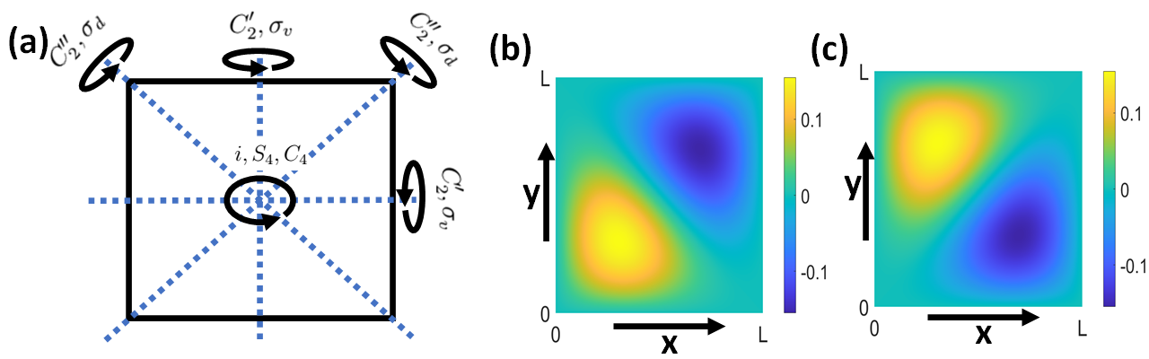
The symmetry of a system is paramount in understanding its mathematical structure. In the classical systems symmetry of the system defines conserved quantities (Noether’s theorem) and in quantum mechanics it translates into the conserved quantum numbers. For example one of the most important result in condensed matter physics is the Bloch’s theorem which states that in a periodic crystal the crystal momentum is conserved and eigenstates of the system is associated with a specific crystal momentum. The conservation of crystal momentum is a consequence of translational symmetry of the periodic system.
In quantum mechanics the energies of a system are discrete in general. Degeneracies may arise due to certain symmetry protection or be accidental in nature (which, in turn may or may not reflect some hidden symmetry). The symmetry protected degenerate eigenstates of the quantum system is related to the two or higher dimensional irreducible representation of the symmetry-group of the system. For example a square box can be classified by point group symmetry (see Fig. 2.11(a)), where a point group is a group of symmetry operations which do not alter the position of particular point. Moreover the energies and wavefunctions of particle in a square box is given by the following expression and respectively. So the energy levels for unequal and are two-fold degenerate. This degeneracy is due to two dimensional irreducible representation of the point group . As an example the linear superposition of wave-functions for the states , and , are shown in the figure Fig. 2.11(b). The wave-functions has the same symmetry as the square box. The traces of the matrices correspond to the symmetry operators assuming the wavefunctions as the basis is equal to the characters of representation of the point group as shown below in the table,
| +2 | 0 | -2 | 0 | 0 | -2 | 0 | +2 | 0 | 0 |
So the degeneracy of the states is protected by the symmetry group of the system. Additionally there is an accidental degeneracy between the states , and , .
In crystal there are several point groups associated with different points on the lattice. All these point groups along with the translational symmetries form a group known as space group. There are 32 possible point groups and 230 possible space groups. Moreover it is possible to include time-reversal symmetry operation for a magnetic system, which flips the spins on the sites. Inclusion of antiunitary time-reversal operation extends the 32 point groups into 122 magnetic point group(32 point group, 32 grey group, 58 color point group) and 230 space group into 1651 magnetic space group (230 space group, 230 grey group, 1191 color space group). The degenerate states at the high symmetry points are due to the two or higher dimensional irreducible representations(corepresentation) of the little-group(little-magnetic group), where little-group(little magnetic group) is the point-group(magnetic-point group) valid for the high symmetric point in the Brillouin zone [153, 154, 155, 156]. Sometimes the presence of anti-unitary symmetry in the system gives rise to the Kramers degeneracy if the square of the operator is negative one at certain points of the Brillouin-zone. Sometimes the energies at the Brillouin zone boundary are degenerate, this is due to presence of nonsymmorphic space group. The Herring’s method is useful to show the nonsymmorphic symmetry protection of band degeneracies [157, 158].

Breaking of symmetry plays an important role from fundamental physics to applied physics. For example presence of Higgs boson is a consequence of spontaneous breaking of electroweak symmetry and the fundamental particles gain mass due to interaction with the Higgs boson field. In a similar manner in a magnetic system breaking of inversion symmetry in the lattice introduces DMI(see Eq. 2.4). As an example the DMIon the bonds of the square shaped molecule as in the figure Fig. 2.12(a) is determined here by considering symmetries of the molecule. Firstly the bonds do not posses any inversion symmetry due to two different atoms denoted by blue and red sphere. On the bond-a the DMIis given by,
where, is the horizontal-mirror symmetry operator.
| (2.123) |
Similarly the and components of DMIat all bonds are zero. Further presence of the mirror symmetry at the diagonal of the square structure transforms the DMIon the bond-a to bond-b in the following way,
| (2.124) |
Similarly using other symmetry operators the DMIat other bonds,
| (2.125) |
The figure Fig. 2.12(b) shows the resultant DMIdue to the symmetry of the system.
Chapter 3 Engineering antichiral edgestates in ferromagnetic honeycomb lattices
The results in this chapter is published as D. Bhowmick and P. Sengupta. Antichiral edge states in Heisenberg ferromagnet on a honeycomb lattice. Physical Review B 101, 195133 (2020). DOI: 10.1103/PhysRevB.101.195133
3.1 Introduction
Haldane’s paradigmatic model [8] of tight binding on a honeycomb lattice with complex next-nearest neighbor hopping – constitutes the foundation of many of the electronic topological phases. It has a natural realization in (quasi-) 2D insulating ferromagnets such as [66] and (A=Ba,Cs,K,La) [159] in terms of magnetic excitations called magnons. In many of these materials, the dominant Heisenberg exchange is supplemented by a next-nearest neighbour anti-symmetric DMI. Furthermore these systems can be described by two species of quasi-particles known as spinons with up and down spins. The spin model translates into the Kane Mele model for spinons – has been proposed to describe the dynamics of the system for a wide range of temperatures [70]. The spinonbands acquire a non-trivial topology due to Berry phase arising from the DMI. This results in a spin Nernst effect (SNE) where a thermal gradient drives a transverse spin current, a spinonversion of the spin Hall effect [70, 160, 161, 71]. In a finite sample, the up(or down) spinonspecies generate two counter propagating spin currents along the edges that are protected by chiral symmetry of the Hamiltonian – analogous to two copies of the thermal Hall effect (THE) of magnons that has been observed in many insulating magnets [42, 150, 43, 162].
Recently, there has been growing interest in engineering systems with co-propagating edge currents [72, 163, 164], through an ingenious, yet physically unrealistic, modification of the Haldane model. The conservation of net current is satisfied by counter propagating bulk current. So in contrast to conventional topological insulators the bulk is not insulating anymore. In this work, we demonstrate that anti-chiral states arise naturally in spinons on a honeycomb magnet comprised of two different magnetic ions, with unequal DMIfor the two sublattices. In the absence of DMI, the spinondispersion consists of two doubly degenerate bands with linear band crossings at K and K′ [62]. The degeneracy between the two spinonbranches are lifted for a finite symmetric DMI [64, 165, 166]. For asymmetric DMI, The two bands for each spinonspecies are shifted in opposite directions relative to each other at the K and K′ points in the Brillouin zone. As a consequence gapless edge modes in up-spinonor down-spinonsector achieve similar dispersion at both edges, giving rise to co-propagating edge states for each spinon-sectors. The spin current due to up-spinonand down-spinonchannels at a particular edge are in opposite directions. Thus the two edges contribute to the net flow of spin-momentum in the same direction (see Fig. 3.3(b)). So, this yields effective anti-chiral edge states for the spinons in addition to normal chiral ones. We present a detailed characterization of the nature of the edge and bulk spinonstates and suggest suitable experimental signatures to detect these novel topological states.
3.2 Model
We consider a Heisenberg ferromagnet on the honeycomb lattice with unequal DMI( and ) on the two sub-lattices. Introducing the symmetric and anti-symmetric combinations of and as, , – termed chiral and anti-chiral DMIrespectively for reasons that will become clear later – the Hamiltonian is given by,
| (3.1) |
where, is the nearest neighbor Heisenberg interaction and when and are along the cyclic arrows shown in Fig. 3.1(b). Again, and denote the nearest-neighbour and next-nearest neighbour bonds respectively. Moreover, () represents the next-nearest neighbour bonds with among sublattice-A (sublattice-B). Finally, for sublattice-A and for sublattice-B (Fig. 3.1(c)). The zero-temperature ground state of the Hamiltonian (Eq. 3.1) is ferromagnetic for in absence of magnetic field. The magnetic field is introduced in a Zeeman coupling term to stabilize the ferromagnetic ground state at finite temperature. The energy scale is set by choosing – all other parameters in the Hamiltonian are in units of .

3.3 Results
3.3.1 Spinon-Picture
The Hamiltonian ( 3.1) has a ferromagnetic ground state. This can be described as the condensation of one of the spin species. At low temperatures (), the only dynamics comes from magnonexcitations that carry the opposite spin. However, at finite temperatures (), both spin species contribute to the dynamics of the system. We start the discussion of our results with the general consideration of both spins contributing to the dynamics and later demonstrate that this naturally reduces to the magnonpicture at low temperatures. We apply the SBMFTto study the topological character of the magnetic system at finite temperatures. A detailed description of SBMFTis given in the section Sec. 2.2.3 in ”Model and Numerical Methods” chapter. The spinonrepresentation consists of the mapping the spin operators into spinons as, , , where and are the annihilation and creation operators of spin-1/2 up or down spinons respectively. The constraint , on the bosonic operators ensures the fulfillment of the spin-S algebra.
Defining the bond-operators, and , we can re-write the Hamiltonian in terms of Schwinger bosons bond operators as,
| (3.2) |
The bond operators is chosen such that the total number of spinonis conserved in the mean field Hamiltoian which is equivalent to -conservation in terms of spin [109]. Furthermore new bond operators are defined so that corresponding mean field parameters are real: , , . is the Lagrange undetermined multiplier introduced to implement the local constraint. We define mean field parameters , , , .
Thus applying Schwinger Boson transformation along with the constraint, and using a mean field approximation to reduce the 4-body operators to bilinear forms, the spin model Eq. 3.1 is mapped to the the mean field hamiltonian,
| (3.3) |
where the mean field parameters are defined as, evaluated on the nearest neighbour-bonds, and , and , evaluated on next nearest neighbour bonds. The terms associated with the parmeters of spinonHamiltonian Eq 3.3 constitute the Kane-Mele model [70]. The term with parameter corresponds to the anti-chiral hopping term introduced in Ref. [72]. The terms with the parameters and have no effect on the energy or the topological character of the bands, as the parameters are found to be much smaller compared to other mean field parameters. The constraint is considered uniform throughout the lattice to retain the translational symmetry of the lattice. Fourier transformation of the mean field Hamiltonian in momentum-space yields,
| (3.4) |
where, . and are the creation operators for spinons on sublattice-A and sublattice-B (see Fig. 3.1(a)), respectively. () represents the Pauli matrices. The other terms are given by,
| (3.5) |
where, and the vectors and are shown in figure Fig. 3.1(a). is the number of unit cells in lattice. is the energy of the ground state and the energies of spinons are considered with respect to the ground state energy. The mean field parameters are obtained by solving a set of self-consistent equations, derived by minimizing the Helmholtz free energy at a particular temperature.
After diagonalizing the k-space Hamiltonian we get,
| (3.6) |
where, the relative energies,
| (3.7) |
refer to the upper () and the lower () band for each spinonsectors .
From this we get the internal energy and the entropy of the non-interacting bosonic system as,
| (3.8) |
where, is the Bose-Einstein distribution of spin-s spinons in the -band. The Helmohltz-free-energy is given by,
| (3.9) |
After minimizing the Helmholtz free energy with respect to the mean field parameters, we get six self consistent equations, given by,
| (3.10) |
The mean field parameters are obtained by solving these six self-consistent equations. It is notable that the mean field parameter can be chosen as real, absorbing the complex phase factor into operator . All other mean field parameters are defined in a way that those are real valued. Using the parameters, we plot the band structure and evaluate corresponding topological information. For a fixed set of , the mean field parameters are solved and plotted against temperature in Fig 3.2. The parameters and represent short range correlations identifying magnetic ordering and serve as order parameters for the transition from paramagnet with short-range correlations to completely uncorrelated paramagnet.

At low temperatures, finite, non-zero values of and denote finite ferromagnetic short-range correlations. A positive determines that the spins are all aligned along the +ve z-direction at . In other words, the system is populated with up-spinons. As the temperature increases, thermally excited down-spinons are generated, resulting in a finite, non-zero . Finally, at high temperatures, a vanishing of all the mean field parameters denotes a transition from paramagnetic phase with finite short range correlations to a totally uncorrelated paramagnetic phase. The paramagnetic phase transition with all zero correlations to be expected to be an outcome of large-N expansion. It has been shown for Heisenberg model that taking into account of the quantum fluctuations in the mean field parameter removes the phase transition [167].

Band structure for spinons at a temperature T=0.25J is shown in Fig. 3.3(a). In the absence of DMI, the two bands cross linearly at the Dirac points K and K′ [62]. A finite DMIopens up a gap with magnitude in each spinonsector at K and K′ [64, 165, 166, 70]. For anisotropic system () considered here, the gap opening is not symmetric and leads to a tilting of the spinonbands near the Dirac momenta. The band tilting for each band in each spinonsector, defined as the energy difference between two Dirac-points in the same band, is given by, . While the anti-chiral DMIdrives the tilting of the bands, it has no effect on the magnitude of the band gap. Crucially, the tilting is opposite for the two species of spinons. For the parameters chosen in Fig. 3.3(a), the gap and tilting for the up-spinonbands are smaller than those for the down spinonbands. This is because in the presence of positive magnetic field considered here, there are fewer down spinons and consequently, .
Nernst effect
The bands in each spinonsector carry non-zero Berry curvature, given by.
| (3.11) |
where represents upper(lower) band and denotes the up-spinon(down-spinon) sector. () is the eigen-vector (energy) of -th band at reciprocal space point- for spinonsetor-. Detecting Berry curvature of spinonbands is more challenging than that for electrons. The absence of Pauli exclusion principle for the (bosonic) quasiparticles as well as their charge neutral character make the standard approaches used for electronic systems inapplicable. Spin Nernst effect has been proposed as a physical phenomenon to identify Berry curvature of spinonbands when there are comparable numbers of up and down spinons. Here we explore whether it can detect the existence of anti-chiral DMI. The Nernst conductivity has been calculated using the equation Eq. 2.112 in the ”Model and Numerical Methods” chapter. The results are plotted in Fig. 3.3(c) for some representative values of and . Increase in increases the band gap as well as the Berry curvature away from the Dirac-points. As a result, the Nernst conductivity is substantially affected by (Fig. 3.3(c)). Conversely, since the Berry curvature is independent of , the anti-chiral DMIhas very little effect in the Nernst conductivity. The effect of on Nernst conductivity can be observed at low temperature due to tilting of the band structure(inset of Fig. 3.3(c)). But at higher temperature, the has no influence in Nernst conductivity, because the contributions from higher bands overshadows the effects of band tilting. So, the presence of in the system is very hard to detect using Nernst conductivity. Instead, we suggest an alternative way to detect the presence of antichiral DMI.
Spin current
The gapped bands are topologically non-trivial with Chern numbers [142]. Due to bulk-edge correspondence, we expect to observe edge states in a finite

system. In the isotropic limit (, i.e., ), the edge states are topologically protected by a chiral symmetry. The spinoncurrents along the two edges are equal and opposite for the up and down spinons. This results in a net flow of spins along the two edges in opposite directions – any scattering to the bulk states is prevented by symmetry constraints. For the asymmetric system considered here, induces an anti-chiral edge current of spinons where each species of spinonflows in the same direction along the two edges. This is balanced by counterflow current of spinons in the opposite direction carried by the bulk modes. The anti-chiral DMIbreaks the chiral symmetry protecting the edge states and enables scattering between edge and bulk states. This edge-to-bulk scattering produces the bulk current that balances the anti-chiral edge current. In the following we discuss how the bulk and edge state dispersion changes due to interplay between the chiral and anti-chiral DMI.
Fig. 3.4 shows the spinonbands for a honeycomb nano-ribbon with dimension lattice sites with zigzag edges, together with the spin current profile along the width of the ribbon. The procedure of numerical calculations for band structures and spin current profile is described in Sec. 2.4.3 in chapter ”Model and Numerical Methods”. Three different sets of are chosen to illustrate the evolution of band dispersion and spin currents with changing DMI. For clarity of presentation, only one species of spinons is shown. Along with the total spin current, the contributions from the bulk and two edge modes are calculated separately to identify the effects of on each component. The spinonbands and the individual spin currents are color coded for easy identification. Green represents the bulk bands and their contribution to the spin current at each position along the width of the ribbon; red (blue) denotes the localized spinonmode and the associated spin current at the top (bottom) edge. A negative (positive) value of the spin current denotes spinontransport to the left (right) along the length of the ribbon.
For , the tilting of the bands is small and the dispersion of edge states at upper and lower edges are opposite, as shown in the Fig. 3.4(b). The edge states are predominantly chiral in nature, and the spin current at the two edges are opposite in direction (Fig. 3.4(c), though not equal in magnitude since breaks chiral symmetry). For large (), the tilting of the bands at the Dirac points is much greater and yields identical dispersion for the two edge states (Fig. 3.4(e)). This results in anti-chiral edge states where the spin current is in the same direction along both edges of the ribbon (Fig. 3.4(f)). Finally, when , one of the edge states (the top edge in the present case) acquires a dispersionless character (Fig. 3.4(h)). In other words, the edge state at the top is localized with no spinontransport while the bottom edge has a finite dispersion with a finite edge current (Fig. 3.4(i)). Because of -symmetry of each spinonsector, there is a counter-propagating bulk current to compensate the imbalance between edge states. The bulk current is not uniform across the width of the ribbon. Instead, it is primarily confined to a small region near the edges. At each edge, the bulk current opposes the edge current, with its magnitude decreasing rapidly away from the edges. To summarize, a non-zero net spin current along the two edges is a definitive signature of the existence of anti-chiral edge states. In principle, the anti-chiral edge states persist over the entire temperature range for which the short range correlations exist for the system (). However, at very high temperature the short range correlations and are very small (see Fig. 3.2), which in turn makes the antichiral edge phenomenon experimentally undetectable at this limits. So we suggest the temperature range is ideal for experimental detection of Anti-chiral edge modes.
3.3.2 Magnon Picture
At low temperature one of the spinonspecies (say, the up-spinon) condense at the lowest energy and form the ferromagnetic ground state. The down-spinons are now excitations above the ground state. In contrast to the high temperature para-magnetic regime, at low temperatures only spin-excitations above the ground state contribute to the dynamics of the system. Thus the system at low temperature can be described more simply using linearized HPbosons, which is given as,
| (3.12) |
where, is the annihilation operator of HPBoson. The HP-transformation is discussed in detail in the section Sec. 2.2.1 in the chapter ”Model and Numerical Method”. The real space Hamiltonian in terms of HPBoson is given by,
| (3.13) |

In Fourier space the Hamiltonian is given by,
| (3.14) |
where, . and are the creation operators for HPBoson on sublattice-A and sublattice-B (see Fig.1(a) of main text), respectively. () represents the Pauli matrices. The other terms are given by,
| (3.15) |
where, and the vectors and are shown in figure Fig.1(a). The magnonHamiltonian is identical to the down-spinonHamiltonian at low temperatures, as the mean field parameters of the spinonHamiltonian reduces to the following values, , , (see Fig. 3.2) and the Lagrange’s undetermined multiplier becomes . In other words, the spinonHamiltonian naturally converges to the magnonHamiltonian at low . The figure Fig. 3.5 shows the results obtained using magnonpicture. The results agree well with those for the down spinonsector in the spinonpicture.
3.3.3 Experimental detection
How does one detect anti-chiral spin currents experimentally? We suggest a suite of experimental probes that, taken together, can provide a ”smoking-gun” signature of the existence of anti-chiral edge states. First, magnetic force microscopy(MFM) offers a promising experimental technique to measure the spinoncurrent across the nano-ribbon and hence can detect the presence of anti-chiral edge states. A non-zero value of net spin current along the two edges provides a direct evidence of anti-chiral edge states. Current MFM techniques can probe the local spin current in a finite sample to a resolution of a few nm. Since the topological character of the spinonbands for the different ranges of anisotropic DMIis reflected in distinct current profile across the ribbon, we believe MFM provides a promising experimental technique to identify anti-chiral edge states in real quasi-2D materials. Second, inelastic neutron scattering spectra can indirectly detect the presence of anti-chiral edge modes, by probing the magnonband structure. If the bands are tilted or the energy at and -point are unequal, it will suggest the presence of anti-chiral edge modes.

Finally, we show that the probing the low energy excitation spectrum offers a powerful probe to detect the asymmetry of the two edges in the limit of , when one of the edge state acquire a dispersionless character compared to the other edge. This low energy spectrum is readily obtained from calculating the DSSF. The DSSFat the edge of a finite system is defined in the equation Eq. 2.114 and the schematic of experimental set-up to measure DSSFvia spin-Hall-noise-spectroscopy is shown in the the figure Fig. 3.6(c) which is further explained in the section Sec. 2.4.5 in ”Model and Numerical Methods” chapter. This experimental technique offers a promising route for detecting anti-chiral edge states. The DSSF (), shown in the figure Fig. 3.6(a)-(b) for different edges, can be interpreted as the number of edge magnons present in a given energy level, and is proportional to the product of the density of states and Bose-Einstein distribution for the corresponding energy level. The signature of the edge states is reflected in the features of the DSSFnear , which is the energy of the edge states in the absence of any DMI. Our results show that is dramatically different for the two edges for strong anti-chiral edge states, viz., when (equivalently or ).
For simplicity, to calculate the dynamical spin structure factor, we have used the HPtransformation as in Eq. 3.12. For the case of ferromagnet with up spin at each site, the HPboson represents the down-spinons in spinonpicture at low temperature. The DSSFis calculated at the edges of the stripe geometry as in figure Fig. 3.4(a). For the site-1 of m-th stripe,
| (3.16) |
where, is the unitary matrix for diagonalization of Hamiltonian and is the bosonic operator after diagonalization and is the periodicity of the stripe along x-direction. The Hamiltonian can be written as,
| (3.17) |
Using the above relation and Heisenberg’s equation of motion it can be proved that,
| (3.18) |
The dynamical spin structure factor is given by,
| (3.19) |
Similarly,
| (3.21) |
3.3.4 Material realization
Symmetry plays an important role in determining the DMIof a spin system as discussed in the section Sec. 2.5. The presence of anti-chiral DMIrequires two in-equivalent sub-lattices in the 2D-honeycomb lattice, as shown in Fig. 3.6(d). The presence of two different types of atoms will result in asymmetric DMI, leading to a broken inversion symmetry and non-zero . Mirror symmetry along the dotted lines prevents any non-zero perpendicular DMIon nearest-neighbour bonds, whereas in-plane mirror symmetry suppresses any in-plane DMI. While we are not aware of any such material at present, the recent discovery of ferromagnetic order in 2D limit of several Cr-based compounds including [66], [168, 169, 170], [170] and [171] as well as the Fe-based family of compounds (A=Ba,Cs,K,La) [159] offer great promise. These quasi-2D materials consist of weakly Van Der Waals-coupled honeycomb ferromagets. Presence of chiral DMIin some members of this family [66]has been established using inelastic neutron scattering spectroscopy. In materials like and , presence of inversion center at the center of honeycomb cell makes the two sub-lattices equivalent. The inversion symmetry can be removed by replacing every other Ge atom by an Si atom as depicted in Fig. 3.6(e). In a similar vein, replacement of P atom by another Group V element in (A=Ba,Cs,K,La) [159] will break the inversion symmetry of the lattice. The breaking of inversion symmetry may, in principle, give rise to additional interactions in these materials, e.g., nearest neighbor DMI. However, we have verified that inclusion of additional interactions, including nearest neighbor DMIas well as 2nd and 3rd nearest neighbor Heisenberg interactions only modifies the linear dispersion of the edge states, and does not suppress the appearance of anti-chiral edge states as shown in the next section.
3.4 Modulation of edge state dispersion in presence of other interactions in a honeycomb ferromagnet

The spin model discussed so far is very ideal. For example, the long range Heisenberg interactions are neglected. Moreover, the criteria to get the anti-chiral DM-term is to break the inversion symmetry at the center of each honeycomb plaquette. The breaking of such symmetry might arise the nearest neighbour out of plane DM-interactions and also in plane DM-interactions. At low temperature, the in plane interactions can be neglected, which gives rise to three magnoninteractions in terms of HPBosons. But, at high temperature, where the spin-system can be treated in terms of spinons, the in plane DM-interaction gives rise to the mixing of two spinonsectors, in presence of which the quasi-particles are mixed eigenstates of spin-up and spin-down sectors. Neglecting, any presence of in plane DM-intration at low temperature, we can re-write a more general Hamiltonian of the material as,
| (3.23) |
where, the DM-interactions and are defined on the nearest neighbour bonds and as shown in Fig. 3.7. Furthermore, single ion anisotropy like terms acts as chemical potential for the spin-excitation, which is taken into account into the magnetic field. To consider more realsitic situation,

we have fixed the Hesenberg interactions present in the material [66], meV, meV, meV. The nearest neighbour DM-terms and magentic field are fixed as meV, meV, meV. We transformed the spin Hamiltonian into magnonHamiltonian using HPtransformation defined in Eq. 3.14. Then, plotted the band structure and dynamical spin structure factor in Fig 3.8. It is noticeable, the qualitative behaviour of the edge states is mostly depend on the DM-interactions and . The presence of other interaction terms in the Hamiltonian just distorts the linear dispersion of the edge states.
3.5 Conclusion
In conclusion, we have studied a Heisenberg ferromagnet with additional next nearest neighbor DMIs on a honeycomb lattice with broken sublattice symmetry. The unequal DMIbetween atoms on different sublattices, together with the broken chiral symmetry results in the emergence of anti-chiral edge states, in addition to the normal chiral modes. This is manifested in unique spin current distribution across the width of a finite system with ribbon geometry. Interestingly, a uncompensated anti-chiral edge current exists, when antichiral DM-interaction is larger than the chiral DM-interaction at a temperature compared to the ferromagnetic Heisenberg interaction (i.e. ). We have shown that the anti-chiral edges states result in a number of observable physical signatures, including a non-zero net spin current along the edges (that is only compensated by counter-flowing bulk spin current) and strong anisotropy in the dynamic spin structure factor at the opposite edges. These unique features serve as smoking-gun signatures for the existence of anti-chiral edge states. We propose experimental probes to detect the presence of anti-chiral edge states via these features as well as a potential material where such states may be realized experimentally. In this work, the stability of the ferromagnetism in the proposed material is not studied. So in future, further studies need to be done to identify the presence of ferromagnetism and anti-chiral DM-interaction in the proposed materials.
Chapter 4 The topological magnon bands in the Flux state in Shastry-Sutherland lattice
The results in this chapter is published as D. Bhowmick and P. Sengupta. Topological magnon bands in the flux state of Shastry-Sutherland lattice model. Physical Review B 101, 214403 (2020). DOI: 10.1103/PhysRevB.101.214403.
4.1 Introduction
Quantum magnets have served as a versatile test bed for realizing novel bosonic phases, including bosonic topological phases. The topological character of the magnetic phase is manifested through the behavior of magnons. Magnons are charge neutral quasi-particle which represent the magnetic excitations of a condensed matter system. Analogous to electrons in standard topological insulators, magnons in magnetic insulators exhibit thermal Hall effect [172], spin-Nernst effect [173, 174, 175], and magnon-driven spin Seebeck effect [176]. The interest in these systems is driven by both fundamental reasons and potential for technological applications. The recent use of Skyrmions in spintronics for efficient magnetic storage and read/write devices with minimal Joule heating effect [177, 178] underscores the potential practical applications of topologically no-trivial magnetic states. The wide range of quantum magnets with varying interactions and lattice structures as well as the ability to control the number of quantized excitations with an external magnetic field make them ideal for exploring novel magnetic phases. Geometrically frustrated quantum magnets are particulalry promising in realizing and controlling topologically non-trivial spin textures [179, 180, 58, 181, 182, 183]. The interplay between competing interactions, geometric frustration and external magnetic field result in a wide variety of magnetic phases that are not commonly observed in their non-frustrated counterparts. In most cases, topological excitations in quantum magnets are driven by DMI [63, 174, 173, 67], although topological magnonbands can exist without DMIas well [180, 51] due to non-coplaner chiral spin-texture. Most strikingly, the change in spin-texture by changing the parameters in the non-coplanar spin systems, gives rise to variety of topological magnonbands in the same system [51, 184].
The SSmodel is a paradigmatic model for the study of frustrated magnetism. Since the degree of frustration can be tuned by varying the ratio of the diagonal and axial bonds, the model exhibits a wide range of novel magnetic phases [185, 186, 187]. The existence of a number of materials with underlying SSgeometry of the magnetic ions offers the prospect of observing theoretically predicted phases and phenomena in real materials [188, 55, 56, 57]. Since DMIis ubiquitous in all of these materials, it is natural to supplement the canonical SSmodel with DMI. This results in an even richer variety of magnetic orderings including collinear, coplanar and non-coplanar spin configurations, several of which host topological magnons [58, 189]. Previous studies of topological magnons for the SSlattice were restricted to the dimer [1] and the ferro-magnetic phases [54]. In recent past there has been a growing interest in studying topological magnons in non-collinear spin configurations in frustrated lattices. Here we present the results of our investigation of topological magnons in the recently proposed flux state, that is stabilised by DMIperpendicular to the lattice plane in the SSlattice [58].In presence of in plane DMI, this evolves to the canted flux state – the resulting magnonbands in an external longitudinal magnetic field, carry non-zero Chern numbers that determine the topological character of the magnonbands. Varying the different components of the DMIresult in a sequence of band topological transitions where the Chern number for the magnonbands change over a wide range of possible values.
The transitions in the band topology of the system can be detected from the first derivative of the thermal Hall conductivity which exhibits a logarithmic divergence at the transition [51, 190]. The peak height of the logarithmic divergence increases with temperature following an algebraic relation. The interpolation of the first derivative of the thermal Hall conductance as a function of temperature yields information on the nature of band touching (gap closing) at the band topological transition.
4.2 Model Hamiltonian and Method

We study a generic microscopic Hamiltonian describing the magnetic properties of the family of SScompounds including the rare earth tetraborides and . We have carefully restricted our choice of Hamiltonian parameters to realistic ranges. We use nearly equal Heisenberg exchange interactions on the diagonal and axial bonds() as observed in the rare earth tetraborides (, R=Er,Tm) [55, 56, 57]. The choice is motivated by the large magnitude of effective localized moments in these compounds which render the HPapproach applicable. The nature of DM-interaction chosen for the study(Fig. 4.1(b)) is based on the symmetry of the SSlattice. We have used a realistic range of the magnitudes of different DM vectors to stabilize the flux state as the magnetic ground state. The possibility of forming Van der Waals heterostructures with heavy metals offers the ability to induce and tune DM interactions over a extended range. The bonds along the two inequivalent diagonals of the unit cell are shifted out of the plane in opposite directions as shown in Fig. 4.1(a) as observed in the canonical SS-compound, in its low temperature phase [99, 191, 1]. The model Hamiltonian is given by,
| (4.1) |
where and () are anti-ferromagnetic Heisenberg spin-exchange on the axial and diagonal bonds of the SSlattice respectively (henceforth referred to as SSbonds). and are DM-vectors on the SSbonds as shown in Fig. 4.1(b). As discussed above, the nature of DM interactions are chosen consistent with the symmetry constraints of the SSlattice Fig. 4.1(a) [1, 87, 88].
We start with a classical ground state and investigate quantized low energy excitations, magnons, focusing on identifying any topological character of the magnonbands. The classical ground state of the Hamiltonian Eq. 4.1 is derived by replacing the local spin moments by classical vectors of unit magnitude. The state of each spin is specified by the polar co-ordinates,
| (4.2) |
The ground state spin configuration is obtained by minimizing the energy of the Hamiltonian w.r.t the angles and . For the ground state phases of interest, viz., the flux and the canted flux states, the magnetic unit cell is of the same size as the unit cell of the SSlattice and consists of four sites as shown in Fig. 4.1.
The classical phases are further discussed in Sec. 4.3. Since we are primarily interested in the flux (Fig. 4.2(a)) and the (in-plane DMI-induced) canted flux states (Fig. 4.3(a)), we start by identifying the parameter ranges where these are realized. The ground state phases of the Hamiltonian Eq.( 4.1) for classical spins has been investigated in Ref. [58] – with vanishing in-plane component of DMI, the flux state (Fig. 4.2(a)) is stabilized above a critical value of the normal component of the DMIalong the axial bonds, (Fig. 4.1(b)) (the DMIon the diagonal bonds are constrained by the symmetry of the lattice to lie on the plane of the lattice). The continuous symmetry of the Hamiltonian is spontaneously broken in the flux state and Fig. 4.2(a) shows one of the degenerate ground states. Interestingly, the flux state state is also realized on the square lattice, but for a much stronger DMI. The geometric frustration of the SSlattice facilitates the appearance of the flux state at a more moderate (and realistic) strength of DM interaction. Moreover, DM-interactions can also be induced by incident circularly polarized optical wave [132], further enhancing the possibility of stabilizing the flux state. However, the symmetry of the SSlattice also allows additional in-plane components of DMI, denoted in this work by on the diagonal bonds and , on the axial bonds (see Fig. 4.1(b)). Any non-zero in-plane DMItilts the spins out of plane keeping the in-plane spin component of nearest-neighbour sites perpendicular to each other. The spins on the two distinct diagonal bonds cant in opposite direction – for one of the diagonals, the spins cant out of the plane, whereas for the other diagonal, they cant into the plane of the lattice. The in-plane components are aligned along the diagonal bonds, as depicted in Fig. 4.3(a). This ground state spin configuration is referred to as the canted-flux state. In the presence of the in-plane components of DMI, the U(1) symmetry of the Hamiltonian is explicitly broken and there is no spontaneous breaking of U(1) symmetry in the in-plane DMIdriven canted flux state. The flux state and canted flux states have not been observed in any real material yet, but recent advances in enhancing DMIby interfacing with heavy-metal thin-films holds the promise to realize such systems in artificial hetero-structures.
To study low energy excitations (magnons) above the magnetic ground state, we have used the linearized HPtransformation [63, 67]. The HPtransformation is a versatile and extensively used approach to study low energy magnons [192, 193, 63, 54, 180, 67, 173, 71, 68]. In this work, we have extended the HPapproach to study magnonexcitations above complex magnetic orders with longer periodicity. Here we present a brief discussion of the method. First, the local co-ordinate axis at each site of the lattice is rotated such that the axis is aligned along the local spin direction. For low temperature excitations the linearized HPtransformation is given by, where, we consider and represent creation (annihilation) operators for quantized excitations above the magnetic ground state at site . These obey bosonic commutation relations, and . Since the unit cell consists of 4 sites, there are four species of bosons corresponding to each inequivalent lattice site. The quadratic magnonHamiltonian is given by,
| (4.3) |
where,
| (4.4) |
where and are the (different) canting angles made by the spins into and out of the plane of the lattice (see Fig. 4.3(a)). The Hamiltonian equation Eq. 4.3 is diagonalized by using Bogoliubov-Valatin transformation as described in section Sec. 2.3.2. In the next section, the detailed classical ground state and corresponding magnonbands and their topological properties are discussed.
4.3 Results and Discussion
4.3.1 Flux State
The flux state is stabilized as the ground state when the component of the DMInormal to the plane of the lattice on the axial bonds, , exceeds a critical magnitude (e.g. when , flux state is stable for ) and the in-plane components vanish for all DMI(the DMIon the diagonal bonds are constrained by symmetry requirements to be strictly in-plane). The flux state is comprised of the nearest-neighbour spins aligned perpendicular to each other and parallel to the plane of the lattice (Fig. 4.2(a)), which is energetically favored by the perpendicular DM-component . The state is characterized by the spontaneous breaking of continuous U(1) spin-rotation symmetry about the z-axis. In the bosonic (magnon) language, the ground state (flux state) is the vacuum and the HPbosons represent quantized low energy excitations above this ground state. The magnonbands at zero magnetic field are shown in the Fig. 4.2(b). At the point the lowest band becomes gapless revealing the presence of Goldstone-mode associated with U(1) symmetry breaking. The bands along line- are

twofold degenerate – these can be understood in terms of Kramer’s degeneracy [68, 194]. The operator commutes with the Hamiltonian where is the reflection operator along the axis and is the translation by have lattice parameter along the same axis, as shown in Fig. 4.2(a); is the time-reversal operator. But, is not the symmetry operator for the classical ground state shown in the Fig. 4.2(a). Instead, symmetry operator for the ground state is given by , which contains an additional rotation of spin by about the axis. On the line- in the Brillouin zone, . Hence is anti-unitary operator with a squared value of , which in turn, results in the Kramer’s degeneracy. maps one Kramer’s degenerate wavefunction along the -line to the other Kramer’s degenerate wavefunction along the -line. Further, the symmetry operation , maps the Kramer’s degenerate state from to , where is the two-fold rotation about the axis and as shown in the Fig. 4.2(a). Thus, the band degeneracy along -line is protected by symmetries and . Additionally, there is four-fold degeneracy at the M-point due to the presence of the symmetry , where is the reflection operator about the axis as shown in Fig. 4.2(a). The symmetry maps one pair of Kramer’s degenerate state to the other pair of Kramer’s degenerate state at M-point. The Berry-curvature is not well defined for bands, because the bands are degenerate.
Application of magnetic field results in a ground state with a finite out of plane spin component, which breaks the -symmetry. The band structure in the presence of an external longitudinal magnetic field is shown in Fig. 4.2(c). The four-fold degeneracy reduces to two fold degeneracy at the M-point, due to the breaking of the -symmetry, as shown in the inset of Fig. 4.2(c). But the band sticking along -line and Goldstone modes at -point are preserved. The degeneracy of the bands prevents the calculation of the standard Berry curvature and Chern numbers of the bands, although there is no symmetry constraints to make Berry curvature zero. One can, however, calculate the non-abelian Berry-curvature and non-abelian Chern number of the degenerate bands following the procedure outlined in Ref. [142](see section Sec. 2.4.2 for details). The results for the non-abelian Berry curvature of the lowest and second-lowest band is shown in Fig. 4.2(d). The negative part of Berry-curvature is highly concentrated at the M-point and the positive berry curvature is distributed in the remaining Brillouin zone. The inversion symmetry of the system with an inversion center at point-c in Fig. 4.2(a) is also reflected in the Berry-curvature. Our results show that the negative and positive contribution of the non-abelian Berry curvature cancels, yielding a vanishing non-abelian Chern number for the lower (or the upper) pair of bands.
4.3.2 Canted flux state
Topological magnonbands and topological phase diagram

When in-plane components of the DM-interactions (both along the axial as well as the diagonal bonds) are included, a canted-flux state, as shown in the Fig. 4.3(a), is realized as the ground state, even in the absence of a magnetic field. The in-plane components of spins are directed along the diagonal bonds; additionally, the spins acquire an out-of-plane component. There is two-fold degeneracy in the ground state configuration – one of them is shown in Fig. 4.3(a) with the spins pointing inwards along the diagonal bonds; the other degenerate state is obtained by flipping the spins so that they point outward along the diagonal bonds and the out-of-plane spin components are also flipped. The spins are canted away of the plane of lattice at an angle given by ,
| (4.5) |
where the spins along one diagonal are canted out of the plane while those along the other diagonal are canted into the plane.
The magnonbands for the zero-field canted-flux state is shown in the Fig. 4.3(b), where the bands are observed to be degenerate at , M and X-point in the Brillouin zone. These degeneracies are protected by symmetries as discussed here. The symmetry protection of the band sticking at X-point in the Brillouin zone in the canted flux state without magnetic field is explained using Herring’s method [157, 158]. The symmetry operators which keep the X-point in the Brillouin zone invariant or change it by a reciprocal lattice vector are,
where,
The symmetry operators , and are mirror reflection along axis-, reflection along axis- and twofold rotation around z-axis at the sublattice-c respectively(Fig. 4.2(a)). The set of translational operators makes the invariant subgroup,
| (4.6) |
where the translational operator follows the constraint at X-point(). Then the factor group can be obtained by deriving the coset of invariant subgroup , where is the set of non-translational symmetry operators which keeps the X-point invariant or change it by reciprocal lattice vector. The factor group is given by,
where , odd and integer. Next, we have derived the character table using package named ”GAP” [195], where the code has been written below, with redefined symbols
The derived character table is given by,
| 1 | 1 | 1 | 1 | 1 | |
| 1 | 1 | -1 | -1 | 1 | |
| 1 | 1 | 1 | -1 | -1 | |
| 1 | 1 | -1 | 1 | -1 | |
| 2 | -2 | 0 | 0 | 0 |
The only valid representation is , since the translational operator should follow the relation,
where, is the identity matrix with a dimension equals to the dimension of representation. Because the only valid representation is which is two dimensional, the bands are doubly degenerate at the X-point. In the similar manner, it can be shown that the degeneracy at the and M-points are also symmetry protected.
In the presence of an external longitudinal magnetic field, the canting angles of the two pairs of spins are no longer identical. The energy of the canted flux state in a magnetic field is given by,
| (4.7) |
where and are the (different) canting angles made by the spins into and out of the plane of the lattice. The energy is minimized for – the application of magnetic field not only lifts the non-symmorphic symmetries but also renders the magnetic symmetry group of the ground state trivial. As a consequence, all the four bands are gapped out, as shown in Fig. 4.3(c). The magnonHamiltonian in presence of all DM-interactions and magnetic field can be found in the equation Eq. 4.3.

The lifting of the symmetry-protected degeneracies in the energy bands allows us to calculate the Berry curvature and Chern number associated with each band separately in the usual manner(see section Sec. 2.4.2). The results reveal that the energy bands acquire topological character for the parameter set chosen in Fig. 4.3. A representative Berry-curvature distribution for the third band is shown in Fig. 4.3(d). The Berry curvature is concentrated near the M and M’ points of the Brillouin zone. The existence of the two-fold rotational symmetry at the center of the diagonal bond is reflected in the Berry-curvature. Unlike the flux state, the Berry curvature across the entire Brillouin zone do not cancel and this results in a non-zero Chern number of the four bands(Fig. 4.3(c))(see section Sec. 2.4.2 for details).
The interplay between competing Heisenberg and DM interactions, together with geometric frustration and external magnetic field results in topologically ordered energy eigenstates. As the relative strengths of the different competing interactions are varied, the energy levels shift and the bands cross / touch in pairs at different points in the Brillouin zone. The accompanying phase transitions are topological in nature as they are characterized by the change in Chern number of the pair of bands involved. By identifying the state of the system with the band topology [180], we find a wide variety of topological magnonbands in different parameter regimes, shown in Fig. 4.4. The four numbers in the figure represent the four Chern numbers from lower to upper magnonbands. The bar above the number denotes the negative Chern number. The color of the boundaries identify the pair of bands involved in the transition. Most strikingly, tuning the strength of the different components of the DMIand applied magnetic field over a small range result in multitude of topologically distinct set of single magnonbands, even though the ground state remains the unaltered (canted flux state). While this is driven by the non-coplanarity of the ground state spin configuration, the exact mechanism of the change in topology of the magnonbands, or their robustness against interaction effects is not clear [180].
Transition in band topology occurs due to gap reopening after closing at the the high symmetry points , X, M and points along line and . Except for the -point, all other k-points in the Brillouin zone can be mapped into another k-point using two-fold rotational symmetry. Thus, the Chern number of the bands changes by , if band touching happens at the -point. It is noticeable that this kind of transition happen in the upper right region of Fig. 4.4(b). Otherwise, the the Chern numbers changes by , because accidental band touching take places at two points in the Brillouin zone due to two-fold rotational symmetry of the system. Most of the topological transition is associated with change in Chern number in Fig. 4.4.
Thermal Hall conductance and its derivative
The non-trivial topology of magnonbands give rise to thermal Hall effect in the magnetic system. The expression of scaled thermal Hall conductivity is given by [196, 197],
| (4.8) |
where is the thermal Hall conductivity, is the scaled temperature, , and is the Bose-Einstein distribution function with as the energy of the -th magnonband at -point in Brillouin zone, is the Berry-curvature of the n-th band at the -point and where is a polylogarithmic function. The scaled temperature , magnonenergies as well as scaled-thermal Hall conductivity are normalized in unit of . The calculation of Berry-curvature is further discussed in section Sec. 2.4.2. In Fig. 4.5(a) and 4.5(b), the results for the scaled thermal Hall conductivity is plotted as a function of Magnetic field and respectively, along the purple lines in Fig. 4.4(b) and Fig. 4.4(d). The different coloured regions in Fig 4.5(a) and 4.5(b) denote distinct topological regions along the purple lines in Fig. 4.4(d) and Fig. 4.4(b) respectively. At the boundary of the different topological regions the band gap closes as shown in the inset of the figures. Generically, band closing occurs at the Dirac point, but sometime a semi-Dirac point is encountered. The type of semi-Dirac point at the boundary between green and purple topological regions in Fig. 4.5(b) is also reported in the reference Ref. [198].
Figs. 4.5(c) and 4.5(d) present the derivative of scaled thermal Hall conductivity with respect to magnetic field and DMI as a function of and the symmetric component of the in-plane DMI respectively. At the boundary between two distinct topological phases, the derivative in the thermal Hall conductance has a logarithmic divergence. The origin of the divergence on the basis of Weyl-point also discussed in Ref. [51]. It is observed from the figures that the logarithmic divergence is universal and independent of the type of band touching. We also have been shown analytically in the next subsections that the nature of divergence is same for tilted Dirac point and Semi-Dirac point. Furthermore, it also can be seen from the figure that the peak height of divergence grows faster, if the band touching happens at the lower pair of bands, due to the larger contribution to the thermal Hall conductivity from magnons in the lower bands. Finally, the sign of the divergence is positive (negative) if Chern number of lower band increases (decreases) at the band topological transition. In the next subsections we show that the nature of logarithmic divergence remain unchanged for different types of band-touching point.

Tilted Dirac point or Generalized Weyl point:
The Hamiltonian corresponds to the tilted Dirac point or generalized Weyl point is given by,
| (4.9) |
where , are the momentum with respect to the band touching point. () are the Pauli’s matrices. is a perturbation to open the gap. denotes the energy of band touching point. The Hamiltonian is general Hamiltonian for any linear dispersions. The energies correspond to the Hamiltonian,
| (4.10) |
where and the corresponding eigenvectors are,
| (4.11) |
where are the normalization constant. The expression of the Berry curvature of the lower band is given by,
| (4.12) |
where Im denotes imaginary part of . Using Eq. 4.9, Eq. 4.10 and Eq. 4.11,
| (4.13) |
Similarly,
| (4.14) |
Using Eq. 4.13 and Eq. 4.14 in Eq. 4.12, the Berry curvature of the lower band,
| (4.15) |
Similarly, for the upper band . The Thermal Hall conductivity expression is given by,
| (4.16) |
Using equations Eq. 4.15 and , we get,
| (4.17) |
From Eq. 4.16, integrating around the band touching points , we get,
| (4.18) |
Semi-Dirac point:
The dispersion of semi-Dirac point,
| (4.19) |
Out of many possibilities, two different possible Hamiltonians are,
| (4.20) |
The Berry curvatures of the both Hamiltonian is given by,
| (4.21) |
Thus, the second Hamiltonian in Eq. 4.20 does not produce any Berry curvature and so topological phase transition can not happen with this kind of Hamiltonian. It can be shown for the first Hamiltonian in equation Eq. 4.20,
| (4.22) |
Particularly, in our study, we got semi-Dirac points with dispersion,
| (4.23) |
Again particularly for phase transition point, near in Fig. 4.5(d) is associated with Semi-Dirac dispersion with , which is also encountered in reference Ref. [198].

Here we show that that the logarithmic divergence follows simple analytical expression as a function of temperature. The main contribution of derivative of thermal Hall conductance comes from the band touching point at energy . Near this point at phase transition the Berry curvature is equal and opposite for the two bands. Near the band touching point,
| (4.24) |
where, . is a constant independent of temperature and proportional to , is a parameter of system(e.g. magnetic field etc.) and is the band topological transition point. Moreover, at a temperature, lower compared with the energy of band touching point, the equation 4.24 transforms into,
| (4.25) |
To demonstrate the validity of Eq. 4.24, we have chosen the band topological transition points near and of Fig. 4.5(c) and Fig. 4.5(d) respectively. The numerically calculation Berry-curvature around the transition point is computationally expensive and in-accurate. So, to correctly calculate the derivative of thermal Hall-conductivity, first the thermal Hall conductivity has been calculated near the transition point and fitted using the expression,
| (4.26) |
where is the band topological transition point. Then the derivative of the expression has been plotted and shown in Fig. 4.6(a) and Fig. 4.6(b). The divergent peak and nearby points increase with the temperature. In Fig. 4.6(c) and 4.6(d), the derivative of conductivity is plotted and fitted as a function of temperature using the Eq. 4.24, considering and as fitting parameter. The band touches at for the band topological transition at in Fig. 4.6(a) and at for the band topological transition at in Fig. 4.6(b). The values of fitting parameter described in Fig. 4.6(c) and Fig. 4.6(d) is quite near the band touching points.
4.4 Conclusion
In conclusion we consider the flux state of SSlattice and showed that in presence of in plane DMIand magnetic field, the system gives rise to non-trivial topological magnonbands. The canted flux state is a non-coplanar spin structure. This leads to a various topologically distinct magnonband structure. Again, we observed the nature of first derivative of thermal Hall conductance is logarithmic divergent at the band topological transition, independent of the type of band touching. We have presented a simple temperature dependent parametric relation for the derivative of thermal Hall conductance, which might be useful to extract the energy of band touching during band topological transition for any generic spin Hamiltonian. We have also suggested an experimental realization of the model studied. In the present work, we have assumed a dilute gas of magnons without any interaction. At finite temperatures, as the density of thermally excited magnons increase, effects of interaction gain importance. Interaction between magnons further re-normalizes the bands and impart a finite life-time, which in turn can change the topological phase diagram obtained in this study. The study of the topological magnonbands for this model in presence of interaction is planned for the future.
Chapter 5 Weyl-triplons in
The results in this chapter is on the arXiv repository as D. Bhowmick and P. Sengupta. Weyl-triplons in . arXiv identifier: arXiv:2004.11551. (under review)
5.1 Introduction
The successful detection of Weyl fermions in TaAs [20], following theoretical prediction of the same [199, 200], marks one of the latest milestones in the study of topological phases of matter, currently the most active frontier in Condensed Matter Physics [201, 202, 203, 204, 205, 206, 207, 21, 208]. Weyl fermions are massless, linearly dispersing quasiparticles with finite chirality, first proposed as solutions to massless Dirac equation in relativistic particle physics [209]. Pairs of Weyl fermions with opposite chirality may combine to form Dirac fermion. In condensed matter systems, non-relativistic analog of Weyl quasiparticles emerge at linear crossing of non-degenerate, topologically protected bands in three dimensional reciprocal space. Interest in these special band crossings have increased since they act as sources of Berry flux and impart topological character to the associated energy bands. Weyl nodes appear in pairs with opposite chirality and can be separated in momentum space in systems with broken time reversal [204, 205, 206, 207] or inversion symmetry [21, 208] or both [210].
The appearance of Weyl points is governed by the geometry of the band structure and symmetries of the Hamiltonian and lattice. As such, it is possible to observe bosonic analogs of Weyl points. This has already been achieved in artificially designed photonic [211, 212, 213, 214] and phononic crystals [215, 216], and proposed for magnons [77, 73, 217, 218, 219, 220]. Weyl-points with toplogical charges are found in the phonon spectra [221, 222] and excitation spectra in phononic [223, 224] and photonic crystals [225, 226] which have no counterpart in high-energy physics. But no such unconventional Weyl-points have been reported in electronic or magnonic systems. Our results reveal that magnetic excitations in the real quantum magnet is a promising platform to realise this unique doubly charged Weyl-points in magnetic excitations for the first time.
Quantum magnets are particularly promising since they have for long been a versatile platform to realise complex quantum states of matter including bosonic analogs of novel fermionic phases. The wide range of available quantum magnets with different lattice geometries and the ability to tune their properties readily by external magnetic field make them ideal testbed for realising bosonic analogs of topological states of matter [63, 227, 54, 193, 228, 89, 68, 70, 229, 230, 231, 232, 233, 234, 77, 73, 217, 218, 219, 220]. However, despite theoretical predictions, experimental observation of Weyl magnons have remained elusive. In this work, we present evidence for the existence of Weyl triplons in the geometrically frustrated Shastry Sutherland compound, . In contrast to previous studies that considered idealized Hamiltonians based on families of quantum magnets [77, 73, 217, 219], we focus on a realistic microscopic Hamiltonian of the extensively studied geometrically frustrated quantum magnet, [1, 87, 88]. In this work, we have used experimentally determined Hamiltonian parameters [235] for the microscopic model that have been demonstrated to reproduce faithfully the experimentally observed behavior of the material [87].
5.2 Results
5.2.1 Microscopic model.
The figure Fig. 5.1(a) illustrates the three dimensional arrangements of Cu-atoms of as a coupled layers of Shastry-Sutherland lattice. The Hamiltonian of the system is given by,
| (5.1) |
where, and denote the summation over the sites belonging to intra-dimer and inter-dimer, bonds respectively in each layer and denotes pairs of adjacent layers. The first four terms describe the intra-layer coupling terms and are depicted in Fig. 5.1(b), where and are the intra-dimer and inter-dimer Heisenberg terms. and denote the intra-dimer and inter-dimer Dzyaloshinskii–Moriya (DM-interaction or DMI). Finally, and are the inter-layer Heisenberg terms and DM-interactions along the green dotted bonds in Fig. 5.1(a). The fifth term is a Zeeman coupling of the spins with a magnetic field perpendicular to the Shastry-Sutherland layer. We include DM-interactions that are symmetry allowed for at temperatures below K [236, 191, 1] in its low-symmetry phase. In-plane components of the inter-layer DM-interaction is neglected, even though it is allowed by the symmetry of the lattice, since it does not contribute to the low energy physics of the magnetic system. The 2D Hamiltonian describing the magnetic properties of each layer have been extensively studied in the past and the

nature of triplon excitations above dimerized ground state and their topological characters delineated using the bond operator formalism [1, 87, 88]. We study the system with additional physically reliable interlayer Heisenberg and DM-interaction terms included in the Hamiltonian. The interlayer DM-interaction shown in Fig. 5.1(c), is taken in the z-direction and also symmetry allowed by the low temperature crystal-symmetry of . For simplicity, we assume . The presence of interlayer DM-interaction drives a variety of topological phases in the system.
5.2.2 Triplon picture.
The ground state is a product of singlet-dimer states on the red and blue-bonds(Fig. 5.1(a)) in a pure Shastry-Sutherland lattice. A singlet state is an entangled state of two spins such that the wave-function is defined by . The lowest excitations above the ground states are direct product of triplets, which are , , . In presence of the small perturbative DM-interaction the ground state is the product state of the rotated-singlets and . The rotated singlets and rotated triplets are related to the original singlet and triplets, as written below,
| (5.2) |
where, . To study the low temperature excitation above the ground state, we used bond operator formalism [99, 1], which is discussed in the section Sec. 2.2.2. In this formalism, we consider the product state of singlets as the vacuum-state and we treat triplets as the quasi-particle excitations named as triplon. The triplon quasi-particles hop around the effective square lattice consisting of two different sub-lattices as shown in Fig. 5.1(d). The low energy effective Hamiltonian in terms of triplons, is further transformed using unitary transformation, such that the two sub-lattices of the effective squared lattice become equivalent. The real-space triplon-Hamiltonian after neglecting the terms of order of is given by,
| (5.3) |
The coupling terms and do not effect the energy of order of magnitude less than . Again the term consists the interaction terms and , such that . The interplay between the DM-interactions and generates different kinds of Weyl-triplons in the system. In the following sub-section, we discuss about the momentum space Hamiltonian and the toplogical Weyl-triplons in the system.
5.2.3 Topological Weyl-triplons.
The momentum space triplon-Hamiltonian is given as,
| (5.4) |
where the matrix is given by,
| (5.5) |
where, , , , . The matrix can be expressed in terms of Gell-Mann matrices,
| (5.6) |
where , , and , , are the Gell-Mann matrices,
| (5.7) |
The eigen-values of the matrix are , and , where . The Gell-Mann matrices span the Lie-algebra of -group. The -matrix of the form in equation Eq. 5.6 contains only Gell-Mann matrices , , , which assures that the for a fixed if the bands are gapped then the Chern-number of the three-bands are of the following form , where is any integer [1, 233]. In this study and so the Chern number from lower to upper band is given by the set .
We study the model fixing the parameters GHz, GHz, GHz and [1, 235] and varying the parameters and . At low energies, the system has three different triplon bands and the possible points at which the band-crossing happens are the high-symmetry points on the - plane, which are , , , . The Weyl-points at the high symmetry points are triply degenerate, which has no equivalence in the high energy physics, because the quasi-paticle excitation triplons in this system do not follow the Poincare symmetry [237, 238].
The schematic figure of different types of Weyl-points in the Brillouin-zone(BZ) is shown in Fig. 5.2(a). The red-dotes illustrates the Weyl-points at positions and , where . The blue dotes denote the Weyl-points at position , where . Again, the green-points are Weyl-points at position , where .

To verify the band crossings are topological Weyl-points, we plot the direction of Berry curvature and change in Chern-number within the first-BZ in Fig. 5.2(b)-(f), for different parameter regions. We note that the Chern number is defined strictly for a two dimensional band; in this study, the Chern number is defined for the lower band in two-dimensional planes at a fixed -value in the 3D Brillouin zone and it is defined for -th band as,
| (5.8) |
where, is -component of Berry-curvature of n-th band (n=1 denotes lowest band) at -point in Brillouin-zone which is given by,
| (5.9) |
where and denote the eigen-value and eigen-state of -th band at -point in Brillouin zone respectively. Three-band tight binding models have previously been studied for two-dimensional systems and found to be have topologically gapped bands with Chern-numbers of three bands or with [233, 1, 239, 240, 241]. In this study, the calculated Chern-numbers of the three gapped bands at a fixed -plane are found to be with or which is similar to the two-dimensional counterpart of the model studied in the reference Ref. [1]. Weyl-points are band-topological transition points in three dimensional Brillouin zone resulting in change in Chern-numbers . It is found that the Chern number changes by for the Weyl-points present at and which indicates that the monopole charge associated with these Weyl-points are . At momenta at and , the Chern-number changes by due to the joint contributions from the Weyl-points , each of which carries a monopole charge of .

Based on the number of Weyl-points and their positions in the - plane, we categorize the - parameter space in to several regions in Fig. 5.3(a). Regions I and II contain no Weyl-points, but in region-II the triplon bands carry non-zero Chern numbers ( and for bands with increasing energy) whereas in region-I, they are topologically trivial. For , the transition in band topology from region-I to region-II occurs at critical magnetic field [1]. The remaining regions III, IV, V and VI feature multiple Weyl points (appearing in pairs), ranging from one pair in region IV to four pairs in region VI. The locations of the Weyl points and their nature are listed in the table in figure Fig. 5.3(b). The Weyl-points at different sub-regions (a), (b), (c), (d) are at the same position but, the monopole charges of some of the Weyl-points change by a sign.

5.2.4 Surface arcs and surface states.
The topological nature of the system is revealed by the presence of the surface states in the material. In Fig. 5.4(a)-(d), we plot the surface spectral function of a slab geometry of a system extended along - direction. Each of the projected bulk Weyl-points on the surface emits two triplon-arcs, which divulge that the monopole charge of a Weyl-point is . The surface triplon-arcs of the system is quite different in the different regions of parameter space, because of the different position and different numbers of Weyl-points present in different sector in the parameter phase. The Fig. 5.4(a), (b), (c), (d) illustrates the surface triplon-arcs for the topological phase regime III, IV, V, VI respectively. For illustration, we describe the Fig. 5.4(a), which corresponds to the region-IIIa in phase diagram Fig. 5.3. There are two-pairs of Weyl-triplon in this region, at positions and . So the projected Weyl-point on the - surface exists at the positions and . The pair of points along axis is connected by two surface triplon-arcs. The existence of surface triplon-arcs in the system can be detected using inelastic neutron scattering. The Fig. 5.4(e)-(h), describes that the surface states are chiral gap-less state present within the bulk gap in the system.
5.2.5 Thermal Hall effect for experimental detection.
Thermal Hall effect is the key experimental signature to detect topological excitations in a magnetic system. The characteristic features of Thermal Hall conductance of an Weyl-magnon is different from the usual gapped topological magnon bands, making it an ideal probe to detect Weyl points. We calculate the thermal Hall effect in different regimes with Weyl points (phases III, IV, V or VI in Fig. 5.3), gapped topological triplons (phases I, II in Fig. 5.3) and gapped topologically trivial triplon excitations to show that the thermal Hall conductivity exhibits distinct features identifying the different regimes. Since the Weyl-points in this system always occur in pairs aligned along the -direction, a transverse current cannot be created along the -axis. Similarly, a temperature gradient along this direction cannot produce a transverse current along any other direction [77]. However, a transverse triplon current can be induced in (or )-direction by applying a temperature gradient along the (or )-direction. The thermal Hall conductance of the system in the plane is given by [41, 197, 196, 141],
| (5.10) |
where is the 2D-thermal Hall conductance contribution from the -plane of fixed -value in the Brillouin Zone, which is given by,
| (5.11) |
where, and , with as bilogarithmic function.

While the nature and magnitude of interlayer DM-interaction () in has not been determined experimentally, it is reasonable to expect finite as its presence is allowed by symmetry of the lattice. We assume a small, but finite, interlayer DMI parallel to the layers (as allowed by the symmetry of the lattice), such that the triplon bands of the system lies in region III(a) of Fig. 5.3. Assuming the thermal Hall conductivity is plotted as a function of magnetic field in Fig. 5.5(a) for . The triplon bands undergo several topological phase transitions in this range of applied field – in Fig. 5.3. The triplon bands in region III(a) contains two pairs of Weyl points at and , while there is one pair of Weyl points at in the region V(a). The triplon bands are fully gapped and topological in nature in region , whereas they are gapped and topologically trivial in region . It is noted that, although the Berry curvature at the Weyl point is ill-defined, the thermal Hall conductance is a continuous function of , because the left and right hand limit and the left hand limit as are equal, where denotes the position of the Weyl-point. The thermal Hall conductance exhibits a unique quasi-linear dependence as a function of magnetic field for a region with Weyl-points, and quite different from the phase region without Weyl points. Moreover the two-dimensional counterpart of the model without inter-layer interaction has no Weyl-points and the thermal Hall conductance for the two-dimensional model does not show any linear dependence as a function of magnetic-field as in figure Fig. 5.5(b). This is because the thermal Hall conductance of magnetic excitations magnons or triplons is proportional to the distance between the Weyl-nodes in momentum space [77], analogous to that of (electrical) Hall conductance observed in Weyl semimetals [242], as a consequence the thermal Hall conductivity exhibits a quasi-linear dependence as a function of magnetic field. In regions III(a) and V(a) the distance between the pair of Weyl-nodes are and respectively. The inset of the Fig. 5.5(a) shows the distance between the Weyl-nodes as a function of magnetic field has point of inflection at the points and , which gives rise to the quasi-linear behaviour of the thermal Hall conductance. To show the quasi-linear dependence of the thermal Hall conductance in Weyl-triplon region as a function of magnetic field, the thermal conductivity is fitted with the analytical expression , where and are fitting parameters and or . The quasi-linear characteristic in thermal Hall conductance in this system is solely due to the presence of the Weyl-nodes. On the other hand, the field dependence of the thermal Hall conductance is markedly different in region were the triplon bands are fully gapped and carry finite Chern numbers, consistent with previous studies [1, 88]. Thus the presence of quasi-linearity in the thermal Hall conductance as a function of magnetic field is a direct evidence of the presence of Weyl-nodes. Finally, in region with topologically trivial, gapped triplon bands, the thermall hall conductivity vanishes.
5.3 Conclusion and Discussion
In conclusion we have demonstrated that is a possible host of Weyl-triplons. Our study shows that interlayer perpendicular DM-interaction (even if very small in magnitude) naturally give rise to the Weyl-triplons. Furthermore the nature of triplon bands at low temperature depends neither on the interlayer Heisenberg interation (because of orthogonal Dimer arrangement) nor on the interlayer in-plane DM-interactions, which makes the appearance of Weyl nodes robust against small deviations from the idealized model. Finally, We have shown that the quasi-linear behaviour of thermal Hall conductance as a function of magnetic field is a possible experimental signature to detect the presence of Weyl nodes.
We also propose neutron scattering experiment as an alternative way to explore the Weyl-nodes in the triplon bands. The neutron scattering spectra is already studied in the reference Ref.[87], which shows that triplon bound state contribution is important under their experimental conditions, which we have neglected in this study. In presence of triplon bound state the three-fold degeneracy is absent at zero magnetic field. But band-topological transitions still exist in the material as a function of magnetic field similar to that reported in Ref.[1] and so the band touching happens as magnetic field is varied. This band touching in 2D model is expected to translate into a Weyl-point in the 3D model in presence of interlayer Dzyaloshinskii–Moriya interaction (DMI). Similar Weyl-triplon phases can also be investigated in the dimer phases of materials [243, 244] and [245].
Chapter 6 Conclusions and future-work
6.1 Conclusions
Throughout this thesis we have considered the two-dimensional Heisenberg model with DMI, which in the LSWT, SBMFTor bond-operator formalism transformed into another bosonic Hamiltonian representing a system of spin-excitations or spin quasi-particles. In this final chapter of the dissertation, we summarize the preceding chapters and present conclusions and outlook. In chapter Ch. 1, we discuss about past studies and the open-questions, which is the starting point of the study. We describe the generic spin models and different methods to study the spin models in chapter Ch. 2. The rest of the section is devoted in the discussion of the chapters Ch. 3, Ch. 4 and Ch. 5, which contains the main findings of our study.
In chapter Ch. 3, we investigate the presence of antichiral edge states in the honeycomb ferromagnets. We find that unequal DMIfor the two sublattices lead to an additional antichiral-DMIand using spinon-picture we determined the temperature range between which the antichiral edge states can be probed experimentally. Antichiral edge states in the system is found when antichiral-DMIis dominant in compared with the chiral-DMI. We show the way to engineer the materials , , (A=Ba, Cs, K, La) to break the inversion symmetry at the center of the hexagon of honeycomb material which in turn induces the antichiral-DMI. Moreover the linear dispersion of antichiral edge states is only distorted in presence of other realistic interactions, but the presence of antichiral edge modes are not destroyed. Moreover we show the possible experimental measurements to explore the existence of antichiral-edge-modes in the material. We investigated that the antichiral DMIdoes not effect the spin Nernst effect qualitatively or quantitatively, thus spin-Nernst effect is not ideal measurement to detect this novel phenomenon. So we proposed some alternative techniques such as magnetic force microscopy, inelastic neutron scattering technique and inverse spin-Hall noise spectroscopy, which are the promising experimental technique to detect the anti-chiral edge states in the system.
In chapter Ch. 4, we studied the topological magnons in the non-coplanar magnetic canted-flux state in the frustrated Shastry-Sutherland lattice. We propose a model spin-Hamiltonian correspond to a distorted rare-earth tetraboride such that in-plane DMIbecome symmetry allowed. In presence of perpendicular DMI(greater than a critical value) and zero in-plane DMIthe ground state is described as a flux state and we find that the magnonbands of this ground state is topologically trivial. But in presence of in-plane DMIalong with out of plane DMIthe magnetic ground state become a non-coplanar canted flux state. In canted flux state, presence of out of plane magnetic field lifts the degeneracy of magnonbands and the gapped out magnonbands are topologically non-trivial due to non-zero Chern number of the bands. We find many band-topological phase transitions in the parameter space due to non-coplanar spin configuration, in-plane DMIand out of plane DMI. The thermal magnonHall effect and non-zero thermal Hall conductance are the signatures for topological magnonbands in different band topological regions. We further show that the derivative of thermal Hall conductance is logarithmic divergent at the band-topological transition point and independent of the type of the band touching point. Moreover we derived a simple analytical expression for derivative of thermal Hall conductance as a function of temperature and propose that fitting of derivative of thermal Hall conductivity with the analytical expression near the band topological transition point gives the energy of the band touching point in experiments.
In chapter Ch. 5 for the first time we show that Weyl-magnetic excitation exists for a dimerized ground states. We propose a extended Shatry-Sutherland lattice with a interlayer coupling and show that is the ideal material for realization of Weyl-triplons. We investigate the whole parameter space of the interlayer DMIand perpendicular magnetic field fixing the other parameter values same as of the material . Any non-zero interlayer perpendicular DMIensures that the triplonexcitations must exhibit a Weyl-triplonand the other realistic interlayer interaction like Heisenberg-interaction and in-plane DMIdo not alter the result. It is found that there are many triplonband topological phases and the phase are categorized by the numbers and positions of the Weyl-triplons present in the system. We show that each Weyl-triploncarries a topological charge . Again Fermi-arc like structure connecting pairs of Weyl-point is also present at the surface of the system denoting the topological Bulk-edge correspondence. Moreover we studied the thermal Hall conductivity as a function of magnetic field. The system undergoes a several topological band transitions as the magnetic field is changed and specifically for the Weyl-triplonregion the thermal Hall conductance has a quasi-linear behaviour, which is a possible experimental signature for Weyl-triplonregion.
In conclusion we investigated various magnetic systems with different lattices to explore the topological magnetic excitations above the ground state. Our result indicates emergence of antichiral edge states in honeycomb ferromagnets, topological magnetic excitations in the flux state of a distorted Shastry-Sutherland lattice and Weyl-triplons in the stacked Shastry-Sutherlnd material . We study different spin models but as well as proposed material realizations and experimental techniques for detection.
6.2 Future-Work
The research in topological magnetic excitation is accelerating in last few years, denoting that there are much more to explore. There are many studies showing the magnonic analogue of phenomena which are generally observed in topological electronic system. For example Hofstadter butterfly [246], Moiré magnons [247] can also observed in the magnetic excitations of the ground state. However further study by varying the magnetic ground state and lattices is necessary to understand the in depth physics. On the other hand Einstein-de Haas effect is theoretically proposed in the magnetic systems due to topological magnons [248]. However the effect is shown to be strong in the ferromagnetically ordered square-octagon lattice system which has no experimental counterpart and thus it is a challenging task to propose a experimentally possible magnetic material with a significant Einstein-de Haas effect. Moreover, the studies of topological magnons are limited to the single-particle treatment of the magnon. At high temperature the magnon-magnon interaction become important and the protection of the edge states against the magnon-magnon interaction is not well studied. The topological protection of the edge states against interaction can be explored by using Landau-Lifsitz-Gilbert equation for ferromagnets [249], whereas a non-equilibrium-Green function technique is suitable for any ground state [250].
The topological magnonincs is a useful branch of magnon based spintronics. But, to improve the applicability of the topological magnonics, it is important to understand how to increase the device efficiency and how to manipulate it externally. DMIis one of the key ingredient for the realization of topological magnon bands. However the magnitude of DMIis quite low for some magnetic system. It is shown that, when a circularly polarized incident perpendicularly on the honeycomb or Kagome lattice Heisenberg magnets, it induces synthetic DMI [251, 252, 253, 254]. Thus circularly polarized light is a useful tool for manipulate a band topological transition. This method can be extended for other lattices for the future work. Another practical limitation of topological magnonic system is the small signal strength from the edge modes and it is theoretically shown that the edge modes can be selectively populated by external light source [255]. This technique of amplification can also be applied in the system studied in this dissertation to understand the mechanism of amplification in each different magnetic system. Magnon based interferometry also become popular [256, 257] and the use of topological systems in magnon interferometry is also needed to be explored. Phonon driven topological magnons is also a interesting phenomena to understand in various systems [231, 232, 233, 234, 258]. Moreover recently the magnon based valleytronics is theoretically proposed [259], however many prospects of the field need to be understood in details.
Chapter A Appendix A : The properties of Schwinger boson bond operators
There are two Schwinger boson bond operators that obeys symmetries of the isotropic Heisenberg Hamiltonian which are discussed in section 2.2.3. The -symmetric bond operators in terms of Schwinger boson operators are of the following form,
| (A.1) |
In this appendix we will discuss the properties of these bond operators.
-symmetry of the bond operators
The derivation is done for spin-half particles and it can be generalized for any spin. A general spin- state can be rotated by an angle about -axis using the following operator,
| (A.2) |
where and are identity operator and y-component of Pauli matrix respectively.
The Schwinger boson operators create the spin up or spin down state operating on a vacuum state basis,
| (A.3) |
So the transformation of operator by rotation of spin about -axis,
Similarly deriving for the operator we get the following sets of relations,
| (A.4) |
Thus,
Using this relations A.4 it is easy to prove that,
| (A.5) |
So the bond operators obeys the -symmetry.
Bond operators as ferromagnetic or antiferromagnetic order parameter
Some basic relations
Before jumping into the derivation, here are some basic relations provided for the derivation. The Schwinger boson transformation is given by,
| (A.6) |
where and are the two species of Schwinger boson at i-th site of the lattice. Using the Schwinger boson transformation the following basic relations are derived,
| (A.7) | ||||
| (A.8) | ||||
| (A.9) | ||||
| (A.10) | ||||
| (A.11) | ||||
| (A.12) |
The relations Eq. A.10, Eq. A.11, Eq. A.12 are equivalent and they are connected by the equation denoting constraint over boson number,
| (A.13) |
For example the equation Eq. A.11 from Eq. A.10 is derived in the following way,
In a similar way we can derive the equation Eq. A.12 by transforming the second and third quartic terms of equation Eq. A.10 using the constraint Eq. A.13.
Bond operators as ferromagnetic order parameter
The -symmetric Schwinger boson bond operators which is suitable for a ferromagnetic phase is given as,
| (A.14) |
So,
Thus the bond operator is related with the ferromagnet order parameter.
Bond operators as antiferromagnetic order parameter
The -symmetric Schwinger boson bond operators which is suitable for a antiferromagnetic phase is given as,
| (A.15) |
So,
Thus the bond operator is related with the antiferromagnet order parameter.
Different forms of isotropic Heisenberg Hamiltonian
A isotropic Heisenberg Hamiltonian is given as,
| (A.16) |
In the previous section we derived,
| (A.17) |
From this we achieve,
| (A.18) |
Chapter B Appendix B : Diagonalization of quadratic Hamiltonianin in k-space
Tight binding Hamiltonian
A tight binding Hamiltonian in k-space can be represented in the following form,
| (B.1) |
where, and is the number of species or degrees of freedom of a particle. is matrix. According to Bloch’s theorem is conserved quantity for a non-interacting system with translational invariance and so after digonalization the Hamiltonian can be written as,
| (B.2) |
where is the creation operator for the single particle state correspond to the energy . The operators after diagonalization can be written as linear superposition of the operators before diagonalization,
| (B.3) |
Using equation Eq. B.2, we prove that,
| (B.4) |
The L.H.S of the equation Eq. B.4,
| L.H.S(B4) | ||||
| (B.5) |
From the R.H.S of the equation Eq. B.4, we get,
| R.H.S(B4) | ||||
| (B.6) |
Equating equations Eq. B.5 and Eq. B.6, we get,
| (B.7) |
Thus the diagonalization of a tight binding Hamiltonian Eq. B.1 is simply a diagonalization problem of matrix .
Bogoliubov Hamiltonian
In this section we show the procedure to diagonalize the Bogoliubov Hamiltonian for the bosons. A general quadratic bosonic Hamiltonian in k-space is given by,
| (B.8) |
Matrix is called the coefficient matrix. The explicit form of the Hamiltonian is given by,
| (B.9) |
According to Bloch’s theorem the diagonalized form of the Hamiltonian is given as,
| (B.10) |
As discussed in the section Sec. 2.3.2, the operator can be expressed as linear combinations of the operators,
| (B.11) |
The equation eq. B.4 is still valid in this case and rewriting the equation,
| (B.12) |
The R.H.S. of the equation Eq. B.12,
| R.H.S(B11) | ||||
| (B.13) |
The L.H.S. of the equation Eq. B.12,
| L.H.S(B11) | ||||
| (B.14) |
Equating Eq. B.13 and Eq. B.14,
| (B.15) |
Thus the dynamic matrix in terms of coefficient matrix is , where,
| (B.16) |
is the identity matrix of size if the coefficient matrix is of dimension . Making complex conjugate of the both sides of equation Eq. B.15, we get,
| (B.17) |
Thus if there is a positive eigen-value present, then a negative eigen-value . Moreover the eigenvectors of the two energies are also related with each other as in equations Eq. B.15 and Eq. B.17. The negative eigenvalues have no physical significance as discussed in the section Sec. 2.3.2. However in numerical calculation presence of the equal negative eigenvalues verifies the correctness of the constructed Hamiltonian. The coefficient matrix should be positive definite (A positive definite matrix is a Hermitian matrix with eigenvalues greater than zero), so that the dynamic matrix to be diagonalizable and that is the reason of the presence of negative and positive eigenvalues.
Furthermore the normalization condition of the eigenvectors can be derived by using the bosonic commutation relation and equation Eq. B.12. The normalization condition is given by,
| (B.18) |
In a same manner using the anti-commutation relations of fermions, a similar Bogolubov-Valatin formalism can be developed and it can be shown that the coefficient matrix and dynamic matrix is same.
Bogoliubov-Valatin transformation of Bosons as para-unitary transformation
In presence of pair-creation and annihilation operator in the Hamiltonian, the Hamiltonian can be represented as,
| (B.19) |
where, is the Nambu-spinor. Here is the set of all annihilation operator.
The Hamiltonian is diagonalized by using para-unitary transformation as,
| (B.20) |
where,
| (B.21) |
where is the number of sub-lattices multiplied by the number of types of bosons at each site. Moreover the para-unitary matrices follow the following rule,
| (B.22) |
using the above relation, we can re-write Eq. B.20 as,
| (B.23) |
Taking the -element of the matrix of the Eq. B.23, we get,
| , | |||
Define and ,
So, we have,
| (B.24) |
The transpose of the equation gives,
| (B.25) |
The completeness relation of the Bogoliubov-Nambu spinors
From Eq. B.22 we get the following ortho-normality relation,
| (B.26) |
Thus, we can expand any state in the Hilbert space as,
| (B.27) |
Multiplying at the both sides,
Using the above equation in Eq. B.27, we get,
So the completeness relation,
| (B.28) |
The equation also can be re-writen as,
| (B.29) |
Chapter C Appendix C : Berry-phase, Berry-curvature and Chern number
Berry-phase in quantum system
The Schrödinger’s equation provides the time-evolution of the wave-function of a system with a Hamiltonian as,
| (C.1) |
The adiabatic process is a slow-process of evolving the Hamiltonian such that the eigenstates do not change and so an n-th eigen-state of the system is an instantaneous eigenstate of the system and follows the equation,
| (C.2) |
where represents the set of time-dependent parameters of the Hamiltonian. The above equation is equivalent to the time-independent Schrödinger’s equation for a time . Differentiating both sides of the equation Eq.C.2 we get,
| (C.3) |
According to adiabatic assumption the state should not change to another state and so which gives,
| (C.4) |
The L.H.S. term is called characteristic time of transition from m-th eigenstate to n-th eigenstate and vice-versa. For an adiabatic process the characteristic time of transition should be zero.
We assume the following ansatz is the solution of the time-dependent Schrödinger’s equation Eq. C.1,
| (C.5) |
Substituting the ansatz into the equation Eq. C.1 we get,
| (C.6) |
According to adiabatic assumption the last term of Eq. C.6 drops out (see Eq. C.5 and Eq. C.4)and the solution of is given by,
| (C.7) |
where,
| (C.8) |
So for an adiabatic process the wavefunction of system gains only a phase factor , which is known as Berry-phase. The berry-phase is independent of time, but depends on the path in the parameter space along which the system evolves, as shown below,
| (C.9) |
where is the path in the parameter space along which the system is evolving.
Phase in Aharnov-Bohm effect
In presence of magnetic vector potential , the time dependent Schrödinger’s equation is,
| (C.10) |
where is a non-electric or non-magnetic potential. Let us assume the solution of the equation in presence of magnetic vector potential,
| (C.11) |
where is the wavefunction in absence of the magnetic vector potential and
| (C.12) |
It is important to note that when the particle moving in a space without a magnetic field i.e. is irrotational. So, is independent of the path of the integration in Eq. C.12 and only a function of position imposing that the gauge of is fixed over the space. Using the Leibniz integral rule, the gradient of is,
| (C.13) |
Taking gradient of both sides of equation Eq. C.10 and using Eq, C.13,
| (C.14) |
Again taking gradient of both sides,
| (C.15) |
Using Eq. C.15 in Eq. C.10 we get,
| (C.16) |
Thus we proved that is the wave-function in absence of magnetic potential. So the relations Eq. C.12 correctly relates the wavefunctions in absence and in presence of magnetic vector potential (note that the magnetic field is considered zero) respectively.
Berry-connection and Berry-curvature in k-space
The derivations in this section are from the reference Ref.[260]. Similar to the Fourier transformation the real-space wave function can be expressed in reciprocal space using Bloch-wave-functions as,
| (C.17) |
Operating position-operator,
Thus the position operator in reciprocal space representation for a particle at -th band in momentum space under adiabatic assumption is given by,
| (C.18) |
The equation of motion of the position operator,
The equation of motion become,
| (C.19) |
Gauge-independent equations for Berry-curvature of 2D-materials
The Berry-curvature for 2D-lattices is,
Because Berry curvature is single component for the case of 2D-materials so we can write down,
| (C.21) |
This formula of Berry curvature is not a gauge independent as discussed in the section Sec. 2.4.2. Using the completeness relation , in the above expression we get,
| (C.22) |
where the summation over is neglected. Because, when , the expression at the R.H.S. become,
where the following equation at the second step is used,
Again we have,
| [Taking derivative of both sides w.r.t ] | |||
| [Multiplying on the both sides] | |||
Similarly we get,
| (C.23) |
Using Eq. C.23 in Eq. C.22, we get,
| (C.24) |
Gauge-independent equations for Berry-curvature for Bogoliubov-Valatin transformation
The Bogoliubov-Valatin transformation is discussed in the section Sec. 2.3.2 and Appendix. B. The expression of the Berry curvature is given by[141],
| (C.25) |
For 2D-lattice, it can be re-written as,
Using the definitions and as in the last subsection of Appendix. B, we get,
| (C.26) |
Using the completeness-relation B.29,
| (C.27) |
The terms are zero and it can be shown using orthonormality relation Eq. 2.61. Using Eq. 2.59,
| [Taking derivative of both sides w.r.t. ] | |||
| [Multiplying on both sides] | |||
| (C.28) |
Similarly,
| (C.29) |
Using Eq. C.29 and Eq. C.28 in Eq. C.27, we get,
| (C.30) |
Chapter D Appendix D : Derivation of thermal Hall conductivity
The out-line of the derivation of thermal Hall conductivity is provided in the section Sec. 2.4.4. In this appendix, the details of the derivation of some specific quantities are given.
Equation of motion of wave-packet
The equation of motion of a wave-packet as in equation Eq. 2.103 is derived by using Lagrangian mechanics. is the envelope function such that the peak of the wave-packet in the real and momentum space are and respectively. Thus can be approximated as and so for an arbitrary function ,
| (D.1) |
The Lagrangian of the system is given by,
One of the equation of motions,
| (D.3) |
Another equation of motion,
| (D.4) |
Thermal Orbital Magnetization due to rotational current along the edge

The origin of the magnetization is schematically shown in the figure Fig. D.1. The thermal orbital magnetization due to motion of wave-packets along the edge is given by,
| (D.5) |
where thermal orbital magnetization from a wave-packet at momentum and at position and at -th band is given by (using equation of motion Eq. D.4),
| (D.6) |
where is the chemical potential. Using the fact that,
| (D.7) |
and using equations D.5 and D.6 and using we get,
| (D.8) |
Chapter E Appendix D : Derivation for spin-Hall-noise-spectroscopy
The out-line of the derivation of spin Hall noise spectrum is provided in the section Sec. 2.4.5. In this appendix, the details of the derivation of some specific equations are given.
spin-Current operator in metal
The interaction between metal and magnet is considered as isotropic Heisenberg interaction,
| (E.1) |
and are the local spin-density operator in metal and spin-operator in magnet respectively. is the electronic field operator in metal and is the vector representing Pauli-matrices. Moreover is the exchange constant and is the lattice scaling in the metal.
Considering the spin-quantization axis in metal (axis for ) aligned along the spin-polarization axis (), the Hamiltonian can be explicitly written as,
| (E.2) |
The spin-current operator for -component of spin is [261],
| (E.3) |
where, .
Derivation for noise spectrum for spin current in metal
The noise spectrum for -component of spin-current in metal is given as,
| (E.4) |
The term can be explicitly given by,
| (E.5) |
where and is the DSSFdefined in equation Eq. 2.114. Moreover the Fourier transformations with periodic boundary condition along direction and open boundary condition along -direction for Green’s functions are defined as,
In a similar way, the term in equation Eq. E.4 can be derived and given by,
| (E.6) |
Using equations Eq. E.4, Eq. E.5, Eq. E.6, we get,
| (E.7) |
The retarded and advanced Green’s function are related to spectral function respectively as [260],
| (E.8) |
where for non-interacting system the spectral function and is the Fermi-Dirac distribution. Using equation Eq. E.8 in equation Eq. E.7 we get,
| (E.9) | ||||
References
- Romhányi et al. [2015] J. Romhányi, K. Penc, and R. Ganesh, Nature Communications 6 (2015), 10.1038/ncomms7805.
- Landau [1937] L. Landau, Zh. Eksp. Teor. Fiz 7, 19 (1937).
- Ginzburg and Landau [1950] V. L. Ginzburg and L. D. Landau, Zh. Eksp. Teor. Fiz. 20, 1064 (1950).
- Klitzing et al. [1980] K. v. Klitzing, G. Dorda, and M. Pepper, Phys. Rev. Lett. 45, 494 (1980).
- Ando et al. [1975] T. Ando, Y. Matsumoto, and Y. Uemura, Journal of the Physical Society of Japan 39, 279 (1975), https://doi.org/10.1143/JPSJ.39.279 .
- Thouless et al. [1982] D. J. Thouless, M. Kohmoto, M. P. Nightingale, and M. den Nijs, Phys. Rev. Lett. 49, 405 (1982).
- Kohmoto [1985] M. Kohmoto, Annals of Physics 160, 343 (1985).
- Haldane [1988] F. D. M. Haldane, Phys. Rev. Lett. 61, 1029 (1988).
- Kane and Mele [2005] C. L. Kane and E. J. Mele, Phys. Rev. Lett. 95, 226801 (2005).
- Bernevig et al. [2006] B. A. Bernevig, T. L. Hughes, and S.-C. Zhang, Science 314, 1757 (2006), https://science.sciencemag.org/content/314/5806/1757.full.pdf .
- König et al. [2007] M. König, S. Wiedmann, C. Brüne, A. Roth, H. Buhmann, L. W. Molenkamp, X.-L. Qi, and S.-C. Zhang, Science 318, 766 (2007), https://science.sciencemag.org/content/318/5851/766.full.pdf .
- Liu et al. [2008] C. Liu, T. L. Hughes, X.-L. Qi, K. Wang, and S.-C. Zhang, Phys. Rev. Lett. 100, 236601 (2008).
- Knez et al. [2011] I. Knez, R.-R. Du, and G. Sullivan, Phys. Rev. Lett. 107, 136603 (2011).
- Hsieh et al. [2008] D. Hsieh, D. Qian, L. Wray, Y. Xia, Y. Hor, R. Cava, and M. Z. Hasan, Nature 452, 970 (2008).
- Hsieh et al. [2009] D. Hsieh, Y. Xia, D. Qian, L. Wray, H. Dil, F. Meier, J. Osterwalder, L. Patthey, J. Checkelsky, N. Ong, A. Fedorov, H.-H. Lin, A. Bansil, D. Grauer, Y. Hor, R. Cava, and M. Z. Hasan, Nature 460, 1101 (2009).
- Xia et al. [2009] Y. Xia, D. Qian, D. Hsieh, L. Wray, A. Pal, H.-H. Lin, A. Bansil, D. Grauer, Y. Hor, R. Cava, and M. Z. Hasan, Nature Physics 5, 398 (2009).
- Hasan and Moore [2011] M. Z. Hasan and J. E. Moore, Annual Review of Condensed Matter Physics 2, 55 (2011), https://doi.org/10.1146/annurev-conmatphys-062910-140432 .
- Ando [2013] Y. Ando, Journal of the Physical Society of Japan 82, 102001 (2013), https://doi.org/10.7566/JPSJ.82.102001 .
- Liu et al. [2014] Z. K. Liu, B. Zhou, Y. Zhang, Z. J. Wang, H. M. Weng, D. Prabhakaran, S.-K. Mo, Z. X. Shen, Z. Fang, X. Dai, Z. Hussain, and Y. L. Chen, Science 343, 864 (2014), https://science.sciencemag.org/content/343/6173/864.full.pdf .
- Lv et al. [2015] B. Q. Lv, H. M. Weng, B. B. Fu, X. P. Wang, H. Miao, J. Ma, P. Richard, X. C. Huang, L. X. Zhao, G. F. Chen, Z. Fang, X. Dai, T. Qian, and H. Ding, Phys. Rev. X 5, 031013 (2015).
- Xu et al. [2015] S.-Y. Xu, I. Belopolski, N. Alidoust, M. Neupane, G. Bian, C. Zhang, R. Sankar, G. Chang, Z. Yuan, C.-C. Lee, S.-M. Huang, H. Zheng, J. Ma, D. S. Sanchez, B. Wang, A. Bansil, F. Chou, P. P. Shibayev, H. Lin, S. Jia, and M. Z. Hasan, Science 349, 613 (2015), https://science.sciencemag.org/content/349/6248/613.full.pdf .
- Kim et al. [2015] Y. Kim, B. J. Wieder, C. L. Kane, and A. M. Rappe, Phys. Rev. Lett. 115, 036806 (2015).
- Fang et al. [2015] C. Fang, Y. Chen, H.-Y. Kee, and L. Fu, Phys. Rev. B 92, 081201 (2015).
- Jin et al. [2019] K.-H. Jin, H. Huang, Z. Wang, and F. Liu, Nanoscale 11, 7256 (2019).
- Levin and Stern [2009] M. Levin and A. Stern, Phys. Rev. Lett. 103, 196803 (2009).
- Maciejko et al. [2014] J. Maciejko, V. Chua, and G. A. Fiete, Phys. Rev. Lett. 112, 016404 (2014).
- Maciejko and Fiete [2015] J. Maciejko and G. A. Fiete, Nature Physics 11, 385–388 (2015).
- Maciejko et al. [2010] J. Maciejko, X.-L. Qi, A. Karch, and S.-C. Zhang, Phys. Rev. Lett. 105, 246809 (2010).
- Raghu et al. [2008] S. Raghu, X.-L. Qi, C. Honerkamp, and S.-C. Zhang, Phys. Rev. Lett. 100, 156401 (2008).
- Rüegg and Fiete [2011] A. Rüegg and G. A. Fiete, Phys. Rev. B 84, 201103 (2011).
- Wang et al. [2015] Y. Wang, Z. Wang, Z. Fang, and X. Dai, Phys. Rev. B 91, 125139 (2015).
- Wen et al. [2010] J. Wen, A. Rüegg, C.-C. J. Wang, and G. A. Fiete, Phys. Rev. B 82, 075125 (2010).
- Maciejko and Rüegg [2013] J. Maciejko and A. Rüegg, Phys. Rev. B 88, 241101 (2013).
- Gong et al. [2014] S.-S. Gong, W. Zhu, and D. N. Sheng, Scientific Reports 4 (2014), 10.1038/srep06317.
- Savary and Balents [2016] L. Savary and L. Balents, Reports on Progress in Physics 80, 016502 (2016).
- Haldane [1983a] F. D. M. Haldane, Phys. Rev. Lett. 50, 1153 (1983a).
- Haldane [1983b] F. Haldane, Physics Letters A 93, 464 (1983b).
- Jolicoeur and Golinelli [2019] T. Jolicoeur and O. Golinelli, Comptes Rendus Chimie 22, 445 (2019), forty years of exchange interactions on the occasion of the 75th birthday of Michel Verdaguer.
- Dzyaloshinsky [1958] I. Dzyaloshinsky, Journal of Physics and Chemistry of Solids 4, 241 (1958).
- Moriya [1960] T. Moriya, Phys. Rev. 120, 91 (1960).
- Katsura et al. [2010] H. Katsura, N. Nagaosa, and P. A. Lee, Phys. Rev. Lett. 104, 066403 (2010).
- Onose et al. [2010] Y. Onose, T. Ideue, H. Katsura, Y. Shiomi, N. Nagaosa, and Y. Tokura, Science 329, 297 (2010).
- Ideue et al. [2012] T. Ideue, Y. Onose, H. Katsura, Y. Shiomi, S. Ishiwata, N. Nagaosa, and Y. Tokura, Phys. Rev. B 85, 134411 (2012).
- Chisnell et al. [2016] R. Chisnell, J. S. Helton, D. E. Freedman, D. K. Singh, F. Demmel, C. Stock, D. G. Nocera, and Y. S. Lee, Phys. Rev. B 93, 214403 (2016).
- Hirschberger et al. [2015a] M. Hirschberger, R. Chisnell, Y. S. Lee, and N. P. Ong, Phys. Rev. Lett. 115, 106603 (2015a).
- Zhang et al. [2020a] H. Zhang, X. Feng, T. Heitmann, A. I. Kolesnikov, M. B. Stone, Y.-M. Lu, and X. Ke, Phys. Rev. B 101, 100405 (2020a).
- Dugaev et al. [2005] V. K. Dugaev, P. Bruno, B. Canals, and C. Lacroix, Phys. Rev. B 72, 024456 (2005).
- Han and Lee [2017] J. H. Han and H. Lee, Journal of the Physical Society of Japan 86, 011007 (2017), https://doi.org/10.7566/JPSJ.86.011007 .
- Owerre [2016] S. A. Owerre, Journal of Physics: Condensed Matter 29, 03LT01 (2016).
- Owerre [2017a] S. A. Owerre, Journal of Physics: Condensed Matter 29, 385801 (2017a).
- Kim et al. [2018] K.-S. Kim, K. H. Lee, S. B. Chung, and J.-G. Park, arXiv e-prints , arXiv:1811.11201 (2018), arXiv:1811.11201 [cond-mat.mes-hall] .
- Lu et al. [2019] Y. Lu, X. Guo, V. Koval, and C. Jia, Phys. Rev. B 99, 054409 (2019).
- Owerre [2017b] S. A. Owerre, Journal of Physics: Condensed Matter 29, 185801 (2017b).
- Malki and Uhrig [2019] M. Malki and G. S. Uhrig, prb 99, 174412 (2019), arXiv:1811.08981 [cond-mat.str-el] .
- Siemensmeyer et al. [2008] K. Siemensmeyer, E. Wulf, H.-J. Mikeska, K. Flachbart, S. Gabáni, S. Mat’a, P. Priputen, A. Efdokimova, and N. Shitsevalova, Phys. Rev. Lett. 101, 177201 (2008).
- Wierschem and Sengupta [2013] K. Wierschem and P. Sengupta, Phys. Rev. Lett. 110, 207207 (2013).
- Ye et al. [2017] L. Ye, T. Suzuki, and J. G. Checkelsky, Physical Review B 95, 174405 (2017), arXiv:1606.04003 [cond-mat.mtrl-sci] .
- Shahzad and Sengupta [2017] M. Shahzad and P. Sengupta, prb 96, 224401 (2017), arXiv:1701.04297 [cond-mat.str-el] .
- Geim and Novoselov [2007] A. Geim and K. Novoselov, Nature materials 6, 183 (2007).
- Owerre [2017c] S. A. Owerre, Journal of Physics Communications 1, 025007 (2017c).
- Kumar et al. [2020] P. S. Kumar, I. F. Herbut, and R. Ganesh, Phys. Rev. Research 2, 033035 (2020).
- Pershoguba et al. [2018] S. S. Pershoguba, S. Banerjee, J. C. Lashley, J. Park, H. Ågren, G. Aeppli, and A. V. Balatsky, Phys. Rev. X 8, 011010 (2018).
- Owerre [2016a] S. A. Owerre, Journal of Physics Condensed Matter 28, 386001 (2016a), arXiv:1602.06772 [cond-mat.str-el] .
- Owerre [2016b] S. A. Owerre, Journal of Applied Physics 120, 043903 (2016b).
- Yuan et al. [2020] B. Yuan, I. Khait, G.-J. Shu, F. C. Chou, M. B. Stone, J. P. Clancy, A. Paramekanti, and Y.-J. Kim, Phys. Rev. X 10, 011062 (2020).
- Chen et al. [2018] L. Chen, J.-H. Chung, B. Gao, T. Chen, M. B. Stone, A. I. Kolesnikov, Q. Huang, and P. Dai, Phys. Rev. X 8, 041028 (2018).
- Owerre [2017] S. A. Owerre, Journal of Applied Physics 121, 223904 (2017), arXiv:1608.00545 [cond-mat.mes-hall] .
- Lee et al. [2018] K. H. Lee, S. B. Chung, K. Park, and J.-G. Park, prb 97, 180401 (2018), arXiv:1712.09801 [cond-mat.mes-hall] .
- Owerre [2016] S. A. Owerre, Phys. Rev. B 94, 094405 (2016).
- Kim et al. [2016] S. K. Kim, H. Ochoa, R. Zarzuela, and Y. Tserkovnyak, prl 117, 227201 (2016).
- Zhang et al. [2018a] Y. Zhang, S. Okamoto, and D. Xiao, Phys. Rev. B 98, 035424 (2018a).
- Colomés and Franz [2018] E. Colomés and M. Franz, Phys. Rev. Lett. 120, 086603 (2018).
- Mook et al. [2016] A. Mook, J. Henk, and I. Mertig, Phys. Rev. Lett. 117, 157204 (2016).
- Li et al. [2016] F.-Y. Li, Y.-D. Li, Y. B. Kim, L. Balents, Y. Yu, and G. Chen, Nature Communications 7 (2016), 10.1038/ncomms12691.
- Jian and Nie [2018] S.-K. Jian and W. Nie, Phys. Rev. B 97, 115162 (2018).
- Mook et al. [2017] A. Mook, J. Henk, and I. Mertig, Phys. Rev. B 95, 014418 (2017).
- Owerre [2018a] S. A. Owerre, Phys. Rev. B 97, 094412 (2018a).
- Hwang et al. [2017] K. Hwang, N. Trivedi, and M. Randeria, “Topological magnons with nodal-line and triple-point degeneracies: Implications for thermal hall effect in pyrochlore iridates,” (2017), arXiv:1712.08170 [cond-mat.str-el] .
- Li and Hu [2017] K.-K. Li and J.-P. Hu, Chinese Physics Letters 34, 077501 (2017).
- Choi et al. [2019] W. Choi, T. Mizoguchi, and Y. B. Kim, Phys. Rev. Lett. 123, 227202 (2019).
- Li et al. [2017] K. Li, C. Li, J. Hu, Y. Li, and C. Fang, Phys. Rev. Lett. 119, 247202 (2017).
- Bao et al. [2018] S. Bao, J. Wang, W. Wang, Z. Cai, S. Li, Z. Ma, D. Wang, K. Ran, Z.-Y. Dong, D. Abernathy, S.-L. Yu, X. Wan, J.-X. Li, and J. Wen, Nature Communications 9 (2018), 10.1038/s41467-018-05054-2.
- Yao et al. [2018] W. Yao, C. Li, L. Wang, S. Xue, Y. Dan, K. Iida, K. Kamazawa, K. Li, C. Fang, and Y. Li, Nature Physics 14, 1011–1015 (2018).
- Zhang et al. [2020b] L.-C. Zhang, Y. A. Onykiienko, P. M. Buhl, Y. V. Tymoshenko, P. Čermák, A. Schneidewind, J. R. Stewart, A. Henschel, M. Schmidt, S. Blügel, and et al., Physical Review Research 2 (2020b), 10.1103/physrevresearch.2.013063.
- Malki et al. [2019] M. Malki, L. Müller, and G. S. Uhrig, Phys. Rev. Research 1, 033197 (2019).
- Joshi and Schnyder [2017] D. G. Joshi and A. P. Schnyder, Phys. Rev. B 96, 220405 (2017).
- McClarty et al. [2017] P. A. McClarty, F. Krüger, T. Guidi, S. F. Parker, K. Refson, A. W. Parker, D. Prabhakaran, and R. Coldea, Nature Physics 13, 736 (2017), arXiv:1609.01922 [cond-mat.str-el] .
- Malki and Schmidt [2017] M. Malki and K. P. Schmidt, Phys. Rev. B 95, 195137 (2017).
- Joshi and Schnyder [2019] D. G. Joshi and A. P. Schnyder, Phys. Rev. B 100, 020407 (2019).
- Anisimov et al. [2019] P. S. Anisimov, F. Aust, G. Khaliullin, and M. Daghofer, Phys. Rev. Lett. 122, 177201 (2019).
- Nawa et al. [2019] K. Nawa, K. Tanaka, N. Kurita, T. J. Sato, H. Sugiyama, H. Uekusa, S. Ohira-Kawamura, K. Nakajima, and H. Tanaka, Nature Communications 10 (2019), 10.1038/s41467-019-10091-6.
- Heisenberg [1928] W. Heisenberg, Journal of Physics 49, 619 (1928).
- Yosida [1997] K. Yosida, “Theory of magnetism,” (Springer-Verlag Berlin Heidelberg, Berlin, Heidelberg, 1997).
- Anderson [1959] P. W. Anderson, Phys. Rev. 115, 2 (1959).
- Sandratskii [2016] L. M. Sandratskii, Phys. Rev. B 94, 184414 (2016).
- Holstein and Primakoff [1940] T. Holstein and H. Primakoff, Phys. Rev. 58, 1098 (1940).
- Sachdev and Bhatt [1990] S. Sachdev and R. N. Bhatt, Phys. Rev. B 41, 9323 (1990).
- Koga et al. [2000] A. Koga, K. Okunishi, and N. Kawakami, Phys. Rev. B 62, 5558 (2000).
- Romhányi et al. [2011] J. Romhányi, K. Totsuka, and K. Penc, Phys. Rev. B 83, 024413 (2011).
- Zhang and Sengupta [2015] Z. Zhang and P. Sengupta, Phys. Rev. B 92, 094440 (2015).
- Ghosh et al. [2016] P. Ghosh, A. K. Verma, and B. Kumar, Phys. Rev. B 93, 014427 (2016).
- Fukumoto [1996] Y. Fukumoto, Journal of the Physical Society of Japan 65, 569 (1996), https://doi.org/10.1143/JPSJ.65.569 .
- De Silva et al. [2002] T. N. De Silva, M. Ma, and F. C. Zhang, Phys. Rev. B 66, 104417 (2002).
- Arovas and Auerbach [1988] D. P. Arovas and A. Auerbach, Phys. Rev. B 38, 316 (1988).
- Sarker et al. [1989] S. Sarker, C. Jayaprakash, H. R. Krishnamurthy, and M. Ma, Phys. Rev. B 40, 5028 (1989).
- Yoshioka [1989] D. Yoshioka, Journal of the Physical Society of Japan 58, 3733 (1989), https://doi.org/10.1143/JPSJ.58.3733 .
- Manuel et al. [1996] L. O. Manuel, C. J. Gazza, A. E. Trumper, and H. A. Ceccatto, Phys. Rev. B 54, 12946 (1996).
- Mondal and Kadolkar [2017] K. Mondal and C. Kadolkar, Physical Review B 95 (2017), 10.1103/physrevb.95.134404.
- Lee et al. [2015] H. Lee, J. H. Han, and P. A. Lee, Phys. Rev. B 91, 125413 (2015).
- Samajdar et al. [2019] R. Samajdar, S. Chatterjee, S. Sachdev, and M. S. Scheurer, Phys. Rev. B 99, 165126 (2019).
- Auerbach [1994] A. Auerbach, “Interacting electrons and quantum magnetism,” (Springer New York, New York, NY, 1994).
- Chalker [2011] J. T. Chalker, Introduction to Frustrated Magnetism: Materials, Experiments, Theory, edited by C. Lacroix, P. Mendels, and F. Mila (Springer Berlin Heidelberg, Berlin, Heidelberg, 2011).
- Auerbach and Arovas [2011] A. Auerbach and D. P. Arovas, “Schwinger bosons approaches to quantum antiferromagnetism,” in Introduction to Frustrated Magnetism: Materials, Experiments, Theory, edited by C. Lacroix, P. Mendels, and F. Mila (Springer Berlin Heidelberg, Berlin, Heidelberg, 2011) pp. 365–377.
- Güçlü et al. [2014] A. D. Güçlü, P. Potasz, M. Korkusinski, and P. Hawrylak, Graphene Quantum Dots (Springer Berlin Heidelberg, Berlin, Heidelberg, 2014).
- Bogolyubov [1947] N. Bogolyubov, J. Phys. (USSR) 11, 23 (1947).
- Bogolyubov [1958a] N. Bogolyubov, J. Exp. Theor. Phys 34, 58 (1958a).
- Bogolyubov [1958b] N. Bogolyubov, Nuovo Cimento 7, 794 (1958b).
- Valatin and Butler [1958] J. Valatin and D. Butler, Nuovo Cim 10, 37 (1958).
- Valatin [1968] J. G. Valatin, “Density matrix methods and superconductivity theory,” in Mathematical Methods in Solid State and Superfluid Theory: Scottish Universities’ Summer School, edited by R. C. Clark and G. H. Derrick (Springer US, Boston, MA, 1968) pp. 194–232.
- Wagner [1986] M. Wagner, Mod. Probl. Condens. Matter Sci. 15, 1 (1986).
- Nambu [2009] Y. Nambu, Rev. Mod. Phys. 81, 1015 (2009).
- Gennes [1966] P.-G. Gennes, “Superconductivity of metals and alloys,” (W.A. Benjamin, New York, 1966).
- wen Xiao [2009] M. wen Xiao, “Theory of transformation for the diagonalization of quadratic hamiltonians,” (2009), arXiv:0908.0787 [math-ph] .
- Peano et al. [2015] V. Peano, M. Houde, C. Brendel, F. Marquardt, and A. Clerk, Nature Communications 7 (2015), 10.1038/ncomms10779.
- Tinkham [1975] M. Tinkham, “Introduction to superconductivity,” (McGraw-Hill, New York, 1975).
- eigenchris [2018] eigenchris, “Tensor calculus 18: Covariant derivative (extrinsic) and parallel transport,” https://www.youtube.com/watch?v=Af9JUiQtV1k#t=33m50s (2018).
- Stoytchev [2017] O. Stoytchev, “From foucault’s pendulum to the gauss–bonnet theorem,” (2017), arXiv:1701.01666 [math.HO] .
- Zwiebach [2019] B. Zwiebach, “Properties of berry’s phase,” https://www.youtube.com/watch?v=RWPfOV0CV5Y&t=330s (2019).
- Chen et al. [2019] H.-T. Chen, C.-H. Chang, and H. chung Kao, “The zak phase and winding number,” (2019), arXiv:1908.06700 [cond-mat.mes-hall] .
- Kregar [2011] A. Kregar, Aharonov-Bohm effect, Lecture note, University of Ljubljana (2011).
- Aharonov and Casher [1984] Y. Aharonov and A. Casher, Phys. Rev. Lett. 53, 319 (1984).
- Owerre [2017a] S. A. Owerre, Journal of Physics Communications 1, 021002 (2017a).
- Chruściński and Jamiołkowski [2004] D. Chruściński and A. Jamiołkowski, Geometric Phases in Classical and Quantum Mechanics (Birkhäuser Boston, Boston, MA, 2004).
- Sheng [2014] T. Z. Sheng, Non-Cyclic Geometric Phase, PhD dissertation, NATIONAL UNIVERSITY OF SINGAPORE (2014).
- Hassan [2012] S. M. Hassan, Berry Phase and Holonomy, Lecture note, School of Science and Engineering , LUMS (2012).
- Lu et al. [2014] L. Lu, J. D. Joannopoulos, and M. Soljačić, Nature Photonics 8, 821–829 (2014).
- Yang et al. [2015] Z. Yang, F. Gao, X. Shi, X. Lin, Z. Gao, Y. Chong, and B. Zhang, Phys. Rev. Lett. 114, 114301 (2015).
- Khanikaev and Shvets [2017] A. Khanikaev and G. Shvets, Nature Photonics 11 (2017), 10.1038/s41566-017-0048-5.
- Ozawa et al. [2019] T. Ozawa, H. M. Price, A. Amo, N. Goldman, M. Hafezi, L. Lu, M. C. Rechtsman, D. Schuster, J. Simon, O. Zilberberg, and I. Carusotto, Rev. Mod. Phys. 91, 015006 (2019).
- Ma et al. [2019] G. Ma, M. Xiao, and C. Chan, Nature Reviews Physics (2019), 10.1038/s42254-019-0030-x.
- Matsumoto et al. [2014] R. Matsumoto, R. Shindou, and S. Murakami, Phys. Rev. B 89, 054420 (2014).
- Fukui et al. [2005] T. Fukui, Y. Hatsugai, and H. Suzuki, Journal of the Physical Society of Japan 74, 1674 (2005), https://doi.org/10.1143/JPSJ.74.1674 .
- D. Mahan [2000] G. D. Mahan, Many-Particle Physics (Springer US, Boston, MA, 2000).
- Laurent [2013] Laurent, “Typical operators in tight binding,” (2013), https://physics.stackexchange.com/q/53270.
- Zhang [2016] L. Zhang, New Journal of Physics 18, 103039 (2016).
- Xiao et al. [2010] D. Xiao, M.-C. Chang, and Q. Niu, Rev. Mod. Phys. 82, 1959 (2010).
- Matsumoto and Murakami [2011a] R. Matsumoto and S. Murakami, Phys. Rev. Lett. 106, 197202 (2011a).
- Sundaram and Niu [1999] G. Sundaram and Q. Niu, Phys. Rev. B 59, 14915 (1999).
- Cooper et al. [1997] N. R. Cooper, B. I. Halperin, and I. M. Ruzin, Phys. Rev. B 55, 2344 (1997).
- Hirschberger et al. [2015b] M. Hirschberger, J. W. Krizan, R. J. Cava, and N. P. Ong, Science 348, 106 (2015b).
- Kovalev and Zyuzin [2016] A. A. Kovalev and V. Zyuzin, Phys. Rev. B 93, 161106 (2016).
- Joshi et al. [2018] D. G. Joshi, A. P. Schnyder, and S. Takei, Phys. Rev. B 98, 064401 (2018).
- Hamermesh [1915] M. Hamermesh, Group theory and its application to physical problems (Dover Publications, United States of America, 1915).
- Newmarch and Golding [1982] J. D. Newmarch and R. M. Golding, Journal of Mathematical Physics 23, 695 (1982), https://doi.org/10.1063/1.525423 .
- Zhang and Liu [2015] R.-X. Zhang and C.-X. Liu, Physical Review B 91 (2015), 10.1103/physrevb.91.115317.
- BRADLEY and DAVIES [1968] C. J. BRADLEY and B. L. DAVIES, Rev. Mod. Phys. 40, 359 (1968).
- Herring [1942] C. Herring, Journal of the Franklin Institute 233, 525 (1942).
- Liao [2012] B. Liao, Nonsymmorphic Symmetries and Their Consequences (2012).
- Kim and Kee [2017] H.-S. Kim and H.-Y. Kee, npj Quantum Materials 2, 20 (2017).
- Zyuzin and Kovalev [2016a] V. A. Zyuzin and A. A. Kovalev, Phys. Rev. Lett. 117, 217203 (2016a).
- Cheng et al. [2016a] R. Cheng, S. Okamoto, and D. Xiao, Phys. Rev. Lett. 117, 217202 (2016a).
- Hentrich et al. [2019] R. Hentrich, M. Roslova, A. Isaeva, T. Doert, W. Brenig, B. Büchner, and C. Hess, Phys. Rev. B 99, 085136 (2019).
- Mandal et al. [2019] S. Mandal, R. Ge, and T. C. H. Liew, Phys. Rev. B 99, 115423 (2019).
- Vila et al. [2019] M. Vila, N. T. Hung, S. Roche, and R. Saito, Phys. Rev. B 99, 161404 (2019).
- Owerre [2017b] S. A. Owerre, Journal of Physics Communications 1, 021002 (2017b).
- Pantaleón et al. [2019] P. A. Pantaleón, R. Carrillo-Bastos, and Y. Xian, Journal of Physics: Condensed Matter 31, 085802 (2019).
- Tchernyshyov and Sondhi [2002] O. Tchernyshyov and S. Sondhi, Nuclear Physics B 639, 429 (2002).
- Samuelsen et al. [1971] E. J. Samuelsen, R. Silberglitt, G. Shirane, and J. P. Remeika, Phys. Rev. B 3, 157 (1971).
- Tsubokawa [1960] I. Tsubokawa, Journal of the Physical Society of Japan 15, 1664 (1960).
- Williams et al. [2015] T. J. Williams, A. A. Aczel, M. D. Lumsden, S. E. Nagler, M. B. Stone, J.-Q. Yan, and D. Mandrus, Phys. Rev. B 92, 144404 (2015).
- Gong et al. [2017] C. Gong, L. Li, Z. Li, H. Ji, A. Stern, Y. Xia, T. Cao, W. Bao, C. Wang, Y. Wang, Z. Qiu, R. Cava, S. G. Louie, J. Xia, and X. Zhang, Nature 546, 265 (2017).
- Murakami and Okamoto [2017] S. Murakami and A. Okamoto, Journal of the Physical Society of Japan 86, 011010 (2017), https://doi.org/10.7566/JPSJ.86.011010 .
- Cheng et al. [2016b] R. Cheng, S. Okamoto, and D. Xiao, Phys. Rev. Lett. 117, 217202 (2016b).
- Zyuzin and Kovalev [2016b] V. A. Zyuzin and A. A. Kovalev, Phys. Rev. Lett. 117, 217203 (2016b).
- Shiomi et al. [2017] Y. Shiomi, R. Takashima, and E. Saitoh, Phys. Rev. B 96, 134425 (2017).
- Jin et al. [2015] H. Jin, S. R. Boona, Z. Yang, R. C. Myers, and J. P. Heremans, Phys. Rev. B 92, 054436 (2015).
- Fert et al. [2013] A. Fert, V. Cros, and J. Sampaio, Nature nanotechnology 8 3, 152 (2013).
- Jonietz et al. [2010] F. Jonietz, S. Mühlbauer, C. Pfleiderer, A. Neubauer, W. Münzer, A. Bauer, T. Adams, R. Georgii, P. Böni, R. Duine, K. Everschor-Sitte, M. Garst, and A. Rosch, Science (New York, N.Y.) 330, 1648 (2010).
- Lee et al. [2008] S. Lee, A. Pirogov, M. Kang, K.-H. Jang, M. Yonemura, T. Kamiyama, S.-W. Cheong, F. Gozzo, N. Shin, H. Kimura, Y. Noda, and J.-G. Park, Nature 451, 805 (2008).
- Owerre [2017] S. A. Owerre, Journal of Physics Condensed Matter 29, 03LT01 (2017), arXiv:1608.08605 [cond-mat.str-el] .
- Tomiyasu et al. [2012] K. Tomiyasu, K. Matsuhira, K. Iwasa, M. Watahiki, S. Takagi, M. Wakeshima, Y. Hinatsu, M. Yokoyama, K. Ohoyama, and K. Yamada, Journal of the Physical Society of Japan 81, 034709 (2012), https://doi.org/10.1143/JPSJ.81.034709 .
- Sagayama et al. [2013] H. Sagayama, D. Uematsu, T. Arima, K. Sugimoto, J. J. Ishikawa, E. O’Farrell, and S. Nakatsuji, Phys. Rev. B 87, 100403 (2013).
- Disseler [2014] S. M. Disseler, Phys. Rev. B 89, 140413 (2014).
- Laurell and Fiete [2018] P. Laurell and G. A. Fiete, prb 98, 094419 (2018), arXiv:1804.09783 [cond-mat.str-el] .
- Miyahara and Ueda [1999] S. Miyahara and K. Ueda, Phys. Rev. Lett. 82, 3701 (1999).
- Koga and Kawakami [2000] A. Koga and N. Kawakami, Phys. Rev. Lett. 84, 4461 (2000).
- Läuchli et al. [2002] A. Läuchli, S. Wessel, and M. Sigrist, Phys. Rev. B 66, 014401 (2002).
- Kageyama et al. [1999] H. Kageyama, K. Yoshimura, R. Stern, N. V. Mushnikov, K. Onizuka, M. Kato, K. Kosuge, C. P. Slichter, T. Goto, and Y. Ueda, Phys. Rev. Lett. 82, 3168 (1999).
- Shahzad and Sengupta [2017] M. Shahzad and P. Sengupta, Journal of Physics: Condensed Matter 29, 305802 (2017).
- Zhang et al. [2010] L. Zhang, J. Ren, J.-S. Wang, and B. Li, Phys. Rev. Lett. 105, 225901 (2010).
- Sparta et al. [2001] K. Sparta, G. J. Redhammer, P. Roussel, G. Heger, G. Roth, P. Lemmens, A. Ionescu, M. Grove, G. Güntherodt, F. Hüning, H. Lueken, H. Kageyama, K. Onizuka, and Y. Ueda, European Physical Journal B 19, 507 (2001), arXiv:cond-mat/0012383 [cond-mat.str-el] .
- Jolicoeur and Le Guillou [1989] T. Jolicoeur and J. C. Le Guillou, Phys. Rev. B 40, 2727 (1989).
- Kawano and Hotta [2019] M. Kawano and C. Hotta, Phys. Rev. B 99, 054422 (2019).
- Young and Kane [2015] S. M. Young and C. L. Kane, Phys. Rev. Lett. 115, 126803 (2015).
- [195] GAP, GAP – Groups, Algorithms, and Programming, Version 4.10.1, The GAP Group (2019).
- Matsumoto and Murakami [2011b] R. Matsumoto and S. Murakami, Phys. Rev. B 84, 184406 (2011b).
- Matsumoto and Murakami [2011c] R. Matsumoto and S. Murakami, Phys. Rev. Lett. 106, 197202 (2011c).
- Wu [2014] Y. Wu, Opt. Express 22, 1906 (2014).
- Weng et al. [2015] H. Weng, C. Fang, Z. Fang, B. A. Bernevig, and X. Dai, Phys. Rev. X 5, 011029 (2015).
- Huang et al. [2015] S.-M. Huang, S.-Y. Xu, I. Belopolski, C.-C. Lee, G. Chang, B. Wang, N. Alidoust, G. Bian, M. Neupane, C. Zhang, S. Jia, A. Bansil, H. Lin, and M. Z. Hasan, Nature Communications 6, 7373 (2015).
- Liu et al. [2019] D. F. Liu, A. J. Liang, E. K. Liu, Q. N. Xu, Y. W. Li, C. Chen, D. Pei, W. J. Shi, S. K. Mo, P. Dudin, T. Kim, C. Cacho, G. Li, Y. Sun, L. X. Yang, Z. K. Liu, S. S. P. Parkin, C. Felser, and Y. L. Chen, Science 365, 1282 (2019), https://science.sciencemag.org/content/365/6459/1282.full.pdf .
- Belopolski et al. [2019] I. Belopolski, K. Manna, D. S. Sanchez, G. Chang, B. Ernst, J. Yin, S. S. Zhang, T. Cochran, N. Shumiya, H. Zheng, B. Singh, G. Bian, D. Multer, M. Litskevich, X. Zhou, S.-M. Huang, B. Wang, T.-R. Chang, S.-Y. Xu, A. Bansil, C. Felser, H. Lin, and M. Z. Hasan, Science 365, 1278 (2019), https://science.sciencemag.org/content/365/6459/1278.full.pdf .
- Liu et al. [2018] E. Liu, Y. Sun, N. Kumar, L. Muechler, A. Sun, L. Jiao, S.-Y. Yang, D. Liu, A. Liang, Q. Xu, and et al., Nature Physics 14, 1125–1131 (2018).
- Armitage et al. [2018] N. P. Armitage, E. J. Mele, and A. Vishwanath, Rev. Mod. Phys. 90, 015001 (2018).
- Wan et al. [2011] X. Wan, A. M. Turner, A. Vishwanath, and S. Y. Savrasov, Phys. Rev. B 83, 205101 (2011).
- Xu et al. [2011] G. Xu, H. Weng, Z. Wang, X. Dai, and Z. Fang, Phys. Rev. Lett. 107, 186806 (2011).
- Wang et al. [2016] Z. Wang, M. G. Vergniory, S. Kushwaha, M. Hirschberger, E. V. Chulkov, A. Ernst, N. P. Ong, R. J. Cava, and B. A. Bernevig, Phys. Rev. Lett. 117, 236401 (2016).
- Soluyanov et al. [2015] A. Soluyanov, D. Gresch, Z. Wang, Q.-S. Wu, M. Troyer, X. Dai, and B. Bernevig, Nature 527, 495 (2015).
- Weyl [1929] H. Weyl, Z. Phys. 56, 330 (1929).
- Chang et al. [2018] G. Chang, B. Singh, S.-Y. Xu, G. Bian, S.-M. Huang, C.-H. Hsu, I. Belopolski, N. Alidoust, D. S. Sanchez, H. Zheng, H. Lu, X. Zhang, Y. Bian, T.-R. Chang, H.-T. Jeng, A. Bansil, H. Hsu, S. Jia, T. Neupert, H. Lin, and M. Z. Hasan, Phys. Rev. B 97, 041104 (2018).
- Lu et al. [2013] L. Lu, L. Fu, J. D. Joannopoulos, and M. Soljačić, Nature Photonics 7, 294–299 (2013).
- Lu et al. [2015] L. Lu, Z. Wang, D. Ye, L. Ran, L. Fu, J. D. Joannopoulos, and M. Soljaić, Science 349, 622 (2015), https://science.sciencemag.org/content/349/6248/622.full.pdf .
- Goi et al. [2018] E. Goi, Z. Yue, B. P. Cumming, and M. Gu, Laser & Photonics Reviews 12, 1700271 (2018), https://onlinelibrary.wiley.com/doi/pdf/10.1002/lpor.201700271 .
- Vaidya et al. [2020] S. Vaidya, J. Noh, A. Cerjan, and M. C. Rechtsman, “Observation of a charge-2 photonic weyl point in the infrared,” (2020), arXiv:2002.03215 [physics.optics] .
- He et al. [2018] C. He, S.-Y. Yu, H. Ge, H. Wang, Y. Tian, H. Zhang, X.-C. Sun, Y. Chen, J. Zhou, M.-H. Lu, and Y.-F. Chen, Nature Communications 9 (2018), 10.1038/s41467-018-07030-2.
- Xiao et al. [2015] M. Xiao, W.-J. Chen, W.-Y. He, and C. Chan, Nature Physics 11 (2015), 10.1038/nphys3458.
- Owerre [2018b] S. Owerre, Scientific Reports 8 (2018b), 10.1038/s41598-018-28508-5.
- Liu and Shi [2019] T. Liu and Z. Shi, Phys. Rev. B 99, 214413 (2019).
- Owerre [2018c] S. A. Owerre, “Topological transitions of spin-excitations in insulating chiral antiferromagnets,” (2018c), arXiv:1811.01946 [cond-mat.str-el] .
- Su and Wang [2017] Y. Su and X. R. Wang, Phys. Rev. B 96, 104437 (2017).
- Miao et al. [2018] H. Miao, T. T. Zhang, L. Wang, D. Meyers, A. H. Said, Y. L. Wang, Y. G. Shi, H. M. Weng, Z. Fang, and M. P. M. Dean, Phys. Rev. Lett. 121, 035302 (2018).
- Zhang et al. [2018b] T. Zhang, Z. Song, A. Alexandradinata, H. Weng, C. Fang, L. Lu, and Z. Fang, Phys. Rev. Lett. 120, 016401 (2018b).
- He et al. [2020] H. He, C. Qiu, X. Cai, M. Xiao, M. Ke, F. Zhang, and Z. Liu, Nature Communications 11 (2020), 10.1038/s41467-020-15825-5.
- Yang et al. [2019] Y. Yang, H.-x. Sun, J.-p. Xia, H. Xue, Z. Gao, Y. Ge, D. Jia, S.-q. Yuan, Y. Chong, and B. Zhang, Nature Physics 15, 645–649 (2019).
- Hu et al. [2020] M. Hu, K. Ding, T. Qiao, X. Jiang, Q. Wang, S. Zhu, and H. Liu, Commun Phys 3 (2020), 10.1038/s42005-020-00395-1.
- Chang et al. [2017] M.-L. Chang, M. Xiao, W.-J. Chen, and C. T. Chan, Phys. Rev. B 95, 125136 (2017).
- Malz et al. [2019a] D. Malz, J. Knolle, and A. Nunnenkamp, Nature Communications 10 (2019a), 10.1038/s41467-019-11914-2.
- Joshi [2018] D. Joshi, Physical Review B 98 (2018), 10.1103/PhysRevB.98.060405.
- Chisnell et al. [2015] R. Chisnell, J. S. Helton, D. E. Freedman, D. K. Singh, R. I. Bewley, D. G. Nocera, and Y. S. Lee, Phys. Rev. Lett. 115, 147201 (2015).
- Seshadri and Sen [2018] R. Seshadri and D. Sen, Phys. Rev. B 97, 134411 (2018).
- Shen and Kim [2020] P. Shen and S. K. Kim, Phys. Rev. B 101, 125111 (2020).
- Park and Yang [2019] S. Park and B.-J. Yang, Phys. Rev. B 99, 174435 (2019).
- Zhang et al. [2019] S. Zhang, G. Go, K.-J. Lee, and S. K. Kim, “Su(3) topology of magnon-phonon hybridization in 2d antiferromagnets,” (2019), arXiv:1909.08031 [cond-mat.mes-hall] .
- Go et al. [2019] G. Go, S. K. Kim, and K.-J. Lee, Phys. Rev. Lett. 123, 237207 (2019).
- Nojiri et al. [2003] H. Nojiri, H. Kageyama, Y. Ueda, and M. Motokawa, Journal of the Physical Society of Japan 72, 3243 (2003).
- Smith and Keszler [1991] R. W. Smith and D. A. Keszler, Journal of Solid State Chemistry 93, 430 (1991).
- Bradlyn et al. [2016] B. Bradlyn, J. Cano, Z. Wang, M. G. Vergniory, C. Felser, R. J. Cava, and B. A. Bernevig, Science 353 (2016), 10.1126/science.aaf5037, https://science.sciencemag.org/content/353/6299/aaf5037.full.pdf .
- Owerre [2017a] S. A. Owerre, EPL (Europhysics Letters) 120, 57002 (2017a).
- Go et al. [2013] G. Go, J.-H. Park, and J. H. Han, Phys. Rev. B 87, 155112 (2013).
- He et al. [2012] Y. He, J. Moore, and C. M. Varma, Phys. Rev. B 85, 155106 (2012).
- Ohgushi et al. [2000] K. Ohgushi, S. Murakami, and N. Nagaosa, Phys. Rev. B 62, R6065 (2000).
- Zyuzin et al. [2012] A. A. Zyuzin, S. Wu, and A. A. Burkov, Phys. Rev. B 85, 165110 (2012).
- Matan et al. [2010] K. Matan, T. Ono, Y. Fukumoto, T. Sato, J. Yamaura, M. Yano, K. Morita, and H. Tanaka, Nature Physics 6, 865 (2010).
- Hwang et al. [2012] K. Hwang, K. Park, and Y. B. Kim, Physical Review B 86, 214407 (2012).
- Tovar et al. [2009] M. Tovar, K. S. Raman, and K. Shtengel, Physical Review B 79, 024405 (2009).
- Owerre [2018d] S. Owerre, Annals of Physics 399, 93–107 (2018d).
- Li and Cheng [2020] Y.-H. Li and R. Cheng, “Moiré magnons in twisted bilayer magnets with collinear order,” (2020), arXiv:2005.14096 [cond-mat.mes-hall] .
- Li et al. [2020] J. Li, T. Datta, and D.-X. Yao, “Einstein-de haas effect of topological magnons,” (2020), arXiv:2005.10273 [cond-mat.str-el] .
- Rückriegel et al. [2018] A. Rückriegel, A. Brataas, and R. A. Duine, Phys. Rev. B 97, 081106 (2018).
- Zhang et al. [2013] L. Zhang, J. Ren, J.-S. Wang, and B. Li, Phys. Rev. B 87, 144101 (2013).
- Owerre [2018e] S. Owerre, Scientific Reports 8 (2018e), 10.1038/s41598-018-22779-8.
- Owerre [2017b] S. A. Owerre, Journal of Physics Communications 1, 021002 (2017b).
- Owerre [2017c] S. A. Owerre, Journal of Physics Communications 1, 021001 (2017c).
- Owerre et al. [2019] S. A. Owerre, P. Mellado, and G. Baskaran, EPL (Europhysics Letters) 126, 27002 (2019).
- Malz et al. [2019b] D. Malz, J. Knolle, and A. Nunnenkamp, Nature Communications 10 (2019b), 10.1038/s41467-019-11914-2.
- Wang et al. [2018] X. S. Wang, H. W. Zhang, and X. R. Wang, Phys. Rev. Applied 9, 024029 (2018).
- Li et al. [2018] Y.-M. Li, J. Xiao, and K. Chang, Nano Letters 18 (2018), 10.1021/acs.nanolett.8b00492.
- Hübener et al. [2018] H. Hübener, U. De Giovannini, and A. Rubio, Nano Letters 18, 1535 (2018), pMID: 29361223, https://doi.org/10.1021/acs.nanolett.7b05391 .
- Ghader [2020] D. Ghader, “Towards magnon valleytronics,” (2020), arXiv:2003.12791 [cond-mat.mtrl-sci] .
- Sun [2013] K. Sun, Topological insulators Part II: Phase and gauge field, Lecture note, Department of Physics, University of Michigan (2013).
- Zotos et al. [1997] X. Zotos, F. Naef, and P. Prelovsek, Phys. Rev. B 55, 11029 (1997).
- Rastelli [2013] E. Rastelli, Statistical Mechanics of Magnetic Excitations (WORLD SCIENTIFIC, 2013) https://www.worldscientific.com/doi/pdf/10.1142/8189 .