[orcid=0000-0003-3535-3538]
[orcid=0000-0003-3094-8911]
A deep neural network with a custom loss function is trained to efficiently generate ground and
excited wavefunctions for different molecular potentials of interest.
![[Uncaptioned image]](2103.00202v2/figures/graphical_abstract.png)
Deep learning methods for the computation of vibrational wavefunctions
Abstract
In this paper we design and use two Deep Learning models to generate the ground and excited wavefunctions of different Hamiltonians suitable for the study the vibrations of molecular systems. The generated neural networks are trained with Hamiltonians that have analytical solutions, and ask the network to generalize these solutions to more complex Hamiltonian functions. This approach allows to reproduce the excited vibrational wavefunctions of different molecular potentials. All methodologies used here are data-driven, therefore they do not assume any information about the underlying physical model of the system. This makes this approach versatile, and can be used in the study of multiple systems in quantum chemistry.
keywords
machine learning,deep learning ,quantum mechanics ,molecular vibrational potentials1 Introduction
The accurate computation of the eigenstates of a dynamical system is a central problem in physics and computational chemistry. For example, being able to efficiently solve the Schrödinger equation is crucial to determine molecular structural properties and molecular dynamics in any quantum-mechanical scenario [1]. When the size and/or complexity of the system increases, finding such solutions becomes challenging. The usual standard methods [2] are based on the variational principle, which implies that in order to get an approximation to the -th eigenstate, the lower-lying ones should also be calculated. This makes the task particularly demanding when one is interested in excited states. The existence of a large density of states and/or classically chaotic dynamics, as it happens in the molecular rovibrational case [3], as opposed to the molecular Born-Oppenheimer electronic one [2], also significantly contributes to the computational burden [4]. For this reason, many methods have have been proposed in the literature to either approximate the underlying interactions of the system [5, 6] or to numerically approximate the exact Schrödinger equation [7]. These methods are based on finding an appropriate description of the system dynamics.
Another option is the use data-based approaches, which do not rely on information about the underlying physical model of the system, but use only data obtained from observations of the system. An increasingly popular family of these data-based methods is machine learning (ML). Indeed, exciting recent work has been devoted to the use of ML techniques to study partial differential equations [8, 9, 10], such as the Schrödinger equation [11], which are at the core of practically all branches of science.
ML is an emerging mathematical and computer science field of study which aims to give computers the ability to learn from examples and experience, without being explicitly programmed to solve the particular task under study. ML is nowadays present in many areas of technology, and any user of today’s technology heavily benefits from its applications, often without even being aware it. Among the most popular and widespread applications of ML facial recognition technology [9, 12], which allows social media platforms to help users tag and share photos of friends, effective web search [13], which eases the acquirement of information, or self-driving cars [14], which will soon be available to customers, are worth mentioning.
One of the most popular and widespread ML method is Artificial Neural Networks (ANN) [15] [or just Neural Networks (NN)], and in particular Deep Learning (DL) [16, 17]. ANN is a widespread method used for generalization problems, especially for the nonlinear function approximation [18]. An ANN is an information processing paradigm inspired by the way that biological nervous systems, particularly the human brain, process information. These NNs are composed of a large number of interconnected “neurons” or nodes, which work coordinately to solve specific problems. ANN are considered to be deep (DNN) when formed by a large number of neuron layers. In this way, DL consists of using deep ANN as the learning algorithm.
In the field of computational chemistry, ML has been extensively used [19] to solve the electronic [20], and, to a lesser extent, the vibrational Schrödinger equations [21, 22, 23], as well as to compute Born-Oppenheimer potential energy surfaces [24, 25], to design new materials [26, 27], and to elucidate the form of a Hamiltonian from its eigenfunctions (inverse problem) [28, 29]. In the case of the vibrational Schrödinger equation, DL methods have proven to give remarkable results in predicting the ground energy of multiple Hamiltonians [30, 31, 32], but there are no relevant applications to the excited case, which is much more interesting since controlled by anharmonicities and mode couplings, and often give rise to the so-called scarred functions [7].
In this paper, instead of predicting the mean energy of an eigenstate, we will obtain the full wavefunction for such state, which provides full information about the system state. Moreover, instead of only focusing on the ground state of the Hamiltonian, we will also obtain high lying states, which correspond to more complex wavefunction topologies. Two different scenarios will be studied. In the first one, we use polynomial potentials and their associated eigenfunctions to train a neural network. Then, the network is asked to generalize to non-polynomial potentials. In the second scenario, we start by using molecular potentials with analytical eigenstates to train the network, and then test the network with more complex perturbed potentials, which have no analytical solution.
The organization of this paper is as follows. In Sect. 2.1 we introduce the neural network model and training details for random polynomial potentials. Similarly, we present in Sect. 2.2 the neural network model and training details for the molecular potentials under study. The results for both cases are presented and discussed in Sect. 3. Finally, Sect. 4 ends the paper by summarizing the main conclusions of the present work.
2 Models and Methods
In this section we present and discuss the potentials and method used for the two scenarios studied in this paper, i.e., random polynomial potentials (Model I) and coupled Morse potentials applied to the H2O molecule (Model II).
2.1 Model I: Random polynomial potentials
The general goal of this work is to train a NN to generate the ground and excited eigenfunctions of different molecular vibrational Hamiltonians. For this purpose, the NN is trained with Hamiltonians belonging to the same family of functions. Then, we expect our NN to be able to generalize and reproduce the wave functions of Hamiltonians described by more general expressions. In this work, we consider both one-dimensional (1D) and a two-dimensional (2D) potentials. In order to design our model, we need to specify both the training data and the learning algorithm.
In the first place (model I), we will consider that the training data is a set of Hamiltonians with random polynomial potentials of (up to) degree four. That is, for the 1D case
| (1) |
and for 2D
| (2) |
Each Hamiltonian has an associated set of eigenfunctions, which are the solution of the corresponding time-independent Schrödinger equation
| (3) |
which in our case will be obtained with the variational method described below.
Since the kinetic energy operator is the same for all Hamiltonians, we only have to provide the potential function to the NN. This allows to pass an easy representation of the Hamiltonian to the NN. Therefore, the training data consists of a set of pairs , where is the -th training potential and the associated computed wave function. Both, potentials and wave functions, are represented in a grid on a rectangular (or linear) domain, so that is a matrix containing the values of [or for 1D] with belonging to a rectangular lattice (or a closed interval for 1D). Similarly, is a matrix containing the values of in such lattice (or closed interval for 1D).
Once the NN has been trained to reproduce the different wave functions for a polynomial potential for a particular energy vibrational state (either the ground or excited state), we ask the network to reproduce the wave functions for another more general, non-polynomial potential. In this work, we chose to test the network against Morse potentials, which are sufficiently different from the training potentials, and they also adequately represent the potential interaction of a diatomic molecule. We write the Morse potential as
| (4) |
where is the distance between atoms, is the corresponding equilibrium bond distance, is the well depth (defined relative to the dissociated atoms), and is a parameter controlling the “width” of the potential (the smaller is, the deeper the well). This potential approaches zero at and equals at its minimum at . The Morse potential is the combination of a short-range repulsion term (the former) and a long-range attractive term (the latter). The Hamiltonian associated to the Morse potential has analytical solution for the eigenenergies and eigenfunctions , being the corresponding quantum number, which are given by
| (5) |
and
| (6) |
respectively, where:
| (7) |
and is a generalized Laguerre polynomial. Figure 1 shows an example of a Morse potential, together with the eigenfunctions for the first four lowest energy levels.

2.1.1 Data Generation
As explained in section 2.1, the NN model is trained using polynomial potentials up to degree four. To ensure that the eigenstates have discrete energies, and thus are physical bound states (as opposed to continuum states), we impose some restriction properties on the coefficients. In our case, we will make sure that the even terms ( and ) dominate over the odd terms ( and ). Also, we allow the potential to be negative and non-centered by including negative values for and [see Eq. (1)]. Finally, we use small values of the coefficients so that the potential does not achieve very high values, which can lead to numerical instability. The values of (for 1D potentials) and (for 2D potentials), chosen according to the previous conditions, are shown in Table 1.
| min | max | |
| -4.5 | 1.5 | |
| -0.65 | 0.65 | |
| 0.2 | 1.0 | |
| -0.01 | 0.01 | |
| 0 | 0.1 |
| min | max | min | max | min | max | |||
| -3 | 0.1 | 0.2 | 1.0 | 0 | 0.2 | |||
| -0.2 | 0.1 | -0.02 | 0.02 | -0.01 | 0.01 | |||
| -0.2 | 0.1 | -0.01 | 0.01 | 0 | 0.04 | |||
| -0.02 | 0.02 | -0.01 | 0.01 | -0.01 | 0.01 | |||
| -0.05 | 0.05 | -0.01 | 0.01 | 0 | 0.02 |
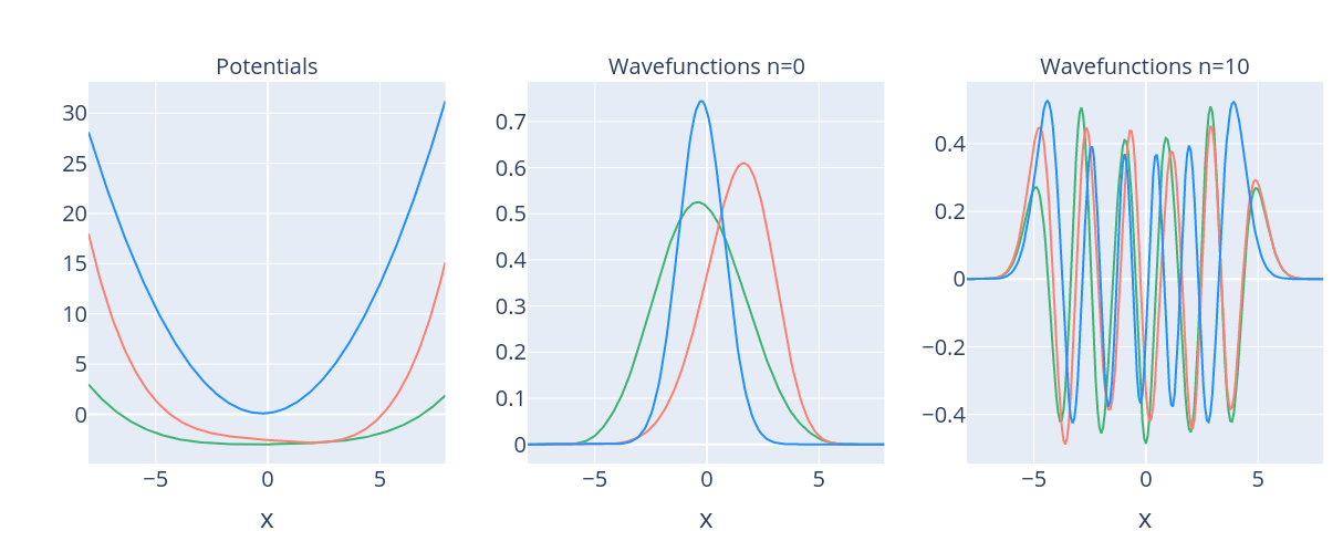
Figure 2 shows some examples of random polynomial potentials and their associated wavefunctions for two values of the vibrational number and .
Apart from the polynomial potentials, the training set also contains the eigenfunctions associated to such Hamiltonians. These random Hamiltonians do not usually have an analytical solution, hence a numerical solver needs to be used. In this work, we use the variational method using harmonic oscillator eigenfunctions as a basis set to generate the eigenfunctions of an arbitrary Hamiltonian . That is, since form a complete basis set for the Hilbert space we can write any wavefunction as a linear combination of the harmonic oscillator eigenfunctions
| (8) |
Therefore, the problem reduces to find the values of which minimize the expected energy
| (9) |
where it is assumed that the eigenfunction is normalized in the standard way, i.e., . For full details of the variational method, and its applications to our 2D potentials, see appendices A and B.
2.1.2 Neural network
In this work, we use NNs as the learning algorithms for both the 1D and 2D problems described above. Here we describe the architecture and learning process in both cases.
For 1D potentials, we use a fully connected neural network (FCNN). The input is an array of 200 points containing the values of the potential in the spatial domain for the fundamental state and for the excited states. Our NN consists of four fully connected layers with 256, 256, 128 and 128 neurons respectively, and RELU activation functions [33]. Every FC layer is followed by a dropout layer with parameter 0.2. These dropout layers help prevent overfitting and thus help the network to generalize to unseen potentials. The output layer is a linear layer with 200 neurons, which predicts the wave function for the given potential. A schematic plot of our FCNN is displayed in Fig. 3 This network is trained using an Adam optimizer [34] with a learning rate of 0.0005 for 1000 iterations. Moreover, we used early stopping to further prevent overfitting the network. The network was trained with 5000 samples with a batch size of 64.


For 2D potentials, we use a convolutional neural network (CNN). This model is used to extract a lower-dimensional embedding of the original data which is then used to make the predictions. CNNs are known to be very useful to extract local patterns from the input data and to extract valuable features for the learning task. The input in this case is a 2D array of size 100100 in the spatial domain . In this case, we use four convolutional layers with 64, 64, 32 and 32 filters respectively. The kernel size is 3 for all four layers, and the stride is (2,2). All activation functions are also RELU here. After each convolutional layer, we add a max-pooling layer to reduce the dimensionality of the embedding. We use a pooling size of (2,2) and a stride of (1,1). Moreover, after each max-pooling layer we add again a dropout layer with parameter 0.2 to avoid overfitting the network. Then, we add 2 fully connected layers with 128 neurons each. The output layer is a linear layer of the same size as the input. The training is performed in the same way as in the 1D case. A schematic representation of the CNN is displayed in Figure 3.
2.2 Model II: Morse potentials
The goal of the second part of the work is to study the performance of a NN trained with the solutions of an analytically solvable Hamiltonian in reproducing the wave functions of the corresponding perturbed non-separable Hamiltonian . For this purpose, let be the Hamiltonian whose eigenfunctions we want to find, and suppose that it can be written à la Kolmogorov-Arnold-Moser [35] as
| (10) |
where is a Hamiltonian whose eigenstates are analytically known. If the “perturbation” is small, then is a good approximation of , and it can be expected that a NN can generalize the wavefunctions for to those for . However, this is not obvious a priori since resonance between modes in the excited states can change significantly the topology of these wavefunctions.
2.2.1 Coupled Morse potentials
We consider the following kinetically coupled 2D Morse oscillator, which has been extensively studied in the past as a model for the stretching vibrations of the H2O molecule [36, 37, 38, 39]
| (11) |
being the -matrix elements equal to
| (12) |
where amu and amu are the H and O atomic masses, respectively, and is the bending angle which in this model is held frozen at 104.5∘. Functions are 1D Morse potentials in the stretching H–O coordinates, and , characterized by parameters and , and are the corresponding conjugate momenta. For the H2O molecule , and therefore is a good approximation of , so that Hamiltonian (11) can be written in the form (10) by making
| (13) |
As explained in the previous section, the way in which we perform our study consists in providing only the potential function to the NN, instead of giving the whole Hamiltonian. This fact allows to have an easy representation of the Hamiltonian as a grid containing the values of the potential energy on a rectangular spatial domain. This representation was possible in the cases presented before in Sect. 2.1.2 because all the Hamiltonians had the same kinetic energy. Nonetheless, our coupled Morse Hamiltonian is different since contains a coupling term in the momentum coordinates and not in the spatial coordinates. Therefore, to be able to provide only the potential energy to the NN, we have to make a change of coordinates in the Hamiltonian in such a way that the coupling appears only in the spatial part, i.e., the potential. To this end, we can rewrite the Hamitonian in generalized coordinates so that the coupling appears in the spatial coordinates instead of in the momentum coordinates.
In order to do so, we apply a canonical transformation to the Hamiltonian obtaining the Hamiltonian . We use a generating function of the form [40], so that
| (14) |
In particular, by choosing of the form
| (15) |
then, the generalized coordinates fulfill the following equations
| (16) |
In this way, the kinetic energy can be written in matrix form as
| (17) |
so that, diagonalizing
| (18) |
Accordingly, defining new coordinates , the new kinetic energy only consists of by diagonal terms
| (19) |
Now, the transformation defined by Eqs. (16) can be used to compute the new set of coordinates
| (20) |
to obtain the new Hamiltonian
| (21) |
Finally, scaling the coordinates so that both particles have the same mass, we define
| (22) |
obtaining the Hamiltonian with the coupling in the spatial coordinates as
| (23) |
Let us remark, that this equivalent Hamiltonian has no kinetic coupling in the momenta and , but it has been moved to the potential term, between spatial coordinates and , which is more adequate for our computational purposes when using NN, as indicated before.
To further illustrate the effect of the above transformation, we compute the Taylor expansion of the new Hamiltonian, thus obtaining
| (24) |
where we see reappearing the two Morse parameters and . We observe that the expansion contains a coupling term , and an anharmonicity in , this indicating that up to order 3 this Hamiltonian is identical to that proposed by Hénon and Heiles to study the stability of some galaxies, at the dawn of nonlinear science [41].
Now that we have defined the coupled Morse potential in generalized coordinates, we have to define the training data of the NN. In this case we use decoupled Morse potentials to train the network, which act as a first order approximation of the coupled Morse potential. The training potentials will then be of the form
| (25) |
where represents a Morse potential with well depth and width . Notice that the Morse parameters of this Hamiltonian are different in each spatial coordinate. The Hamiltonian associated to this potential is separable, and the Schrödinger equation has analytical solution in terms of expressions (5)-(7). Thus, there is no need to use a numerical solver to train the NN, which makes the method more convenient. In this case the training data are pairs , where is a matrix containing the values of the potential in a rectangular domain, and is the associated wavefunction corresponding to the vibrational quantum numbers . We train different models for different quantum numbers in order to reproduce multiple excited eigenstates of the coupled Morse Hamiltonian. Notice that here the excited states are identified by their quantum numbers , instead of their energies . We made this choice because when the difference between eigenenergies is small, the th energy level of two similar potentials can correspond to very different quantum numbers , , and consequently completely different wave functions. This fact would “confuse” the NN since two similar inputs would have very different outputs. In the next section we give further details about how the training data are generated.
2.2.2 Data Generation
Neural networks are useful methods for extracting features of complex data. However, if the training and test sets are too different, the network may not be able to produce good results. For this reason, it is important that the training data resembles as much as possible the test data. In this work we are approximating a coupled Morse Hamiltonian with a separable Morse Hamiltonian [see Eq. (25)]. Two strategies were then used to generate useful training data:
- •
Selecting the Morse parameters , : We selected the parameters of the decoupled potential in two different ways:
- –
By performing curve fitting and finding the parameters , which best approximate the coupled Morse potential in Eq. (10).
- –
By choosing the parameters , which have the same quadratic order Taylor expansion coefficients as the coupled Morse potential. Considering Eq. (24) the choice should be
(26)
In order to obtain the training data we first generated samples of the parameters of the coupled Morse potential , , and then found the decoupled Morse , parameters, according to the previous strategies.
- –
- •
Selecting the and ranges: Once the Morse parameters have been chosen, we try to improve the resemblance with the coupled Morse potential by changing the values of the spatial domains. The input of the NN is a grid containing the values of the potential in a certain spatial domain, but such domain is not specifically given. Therefore, if we change the range of this domain the network will not notice the difference, as long as the number of points remains constant. This fact allows us to stretch the spatial domain so that the decoupled potential is more similar to the coupled potential. We performed a grid search to find the domain ranges which best approximate the coupled potential energy. The only constraint is that in a given spatial domain, the associated wave function fits into that domain. Otherwise, the sample will no be useful for training. Recall that this technique could only be used because the learning algorithm, i.e., the NN is a data-based approach, instead of a model-based approach, which means that uses no information about the underlying physical model of the system.
2.2.3 Neural network
The architecture of the NN in this case is the same as the one used with the 2D random polynomial potentials in Sect. 2.1.2. The only difference in the training process is the choice of the loss function [42]. When the energy of the system increases, the eigenfunctions of the coupled Morse Hamiltonian show significant differences to any of the eigenfunctions of the decoupled Morse Hamiltonian, due to the effect of the different nonlinear resonances existing in the system [36, 37]. For example, the number of nodes of the wavefunction may not be well-defined. In this case, training the neural network with only the decoupled wavefunction does not give optimal results. For this reason, we add a custom loss function to help training the NN, defined in the following way
| (27) |
where is the predicted mean energy, which is calculated using the input potential and the predicted wavefunction . Therefore the total loss function is
| (28) |
where are the wavefunctions of the decoupled Hamiltonian and are the wavefunctions of the coupled Hamiltonian, and . Parameter is chosen so that the two terms of the Schrödinger equation loss have the same order of magnitude. In this case, we choose for all the training process. We train the network for 300 iterations. During the first 100 iterations we set so that the model learns to reproduce the wavefunctions of multiple decoupled Hamiltonians. Then, we choose so that the two loss functions have the same order of magnitude. In this case, we set . Notice that since the decoupled Morse potential already gives a fair approximation of the true wavefunction, we do not need to put any constraints on the energy of the system. The NN converges to the true solution, which follows the Schrödinger equation.
3 Results
3.1 Model I: Polynomial potentials
As described in the previous section, in the first part of this work we use random polynomial potentials and their associated eigenfunctions, to train our NN. Afterwards, we test the ability of the network to generalize to non-polynomial potentials, in particular to the Morse potential.
Two NNs were trained for this purpose, the first one to reproduce the fundamental eigenfunction, and the second to reproduce excited eigenfunctions, which in this case was chosen as that corresponding to . Table 2 shows the mean square error (MSE) obtained for the predicted wavefunctions values and also for the mean energies of such vibrational states. These results are also shown graphically in Figs. 4 and 5 for the fundamental state, and in Figs. 6 and 7 for the excited state.
In the case of the Morse Hamiltonian ground state, the MSE for both energy and wavefunction is similar to those obtained for the polynomial potentials. This fact means that the NN can effectively generalize to non-polynomial potentials when trained with polynomial potentials. The MSE of the harmonic oscillator potentials is also similar to the MSE of the random potentials, which is not an unexpected result since the harmonic oscillator is also a polynomial potential as well. Finally, it should be remarked that, since the MSE of the wave function is similar for all potentials, the NN is not producing much overfitting.
Regarding the excited eigenfunctions, the MSE for both the energy and wave function is small for the three types of potentials. However, we observe that the wave function prediction for the Morse potentials presents higher MSE than the MSE of the polynomial potentials. In particular, Fig. 6 shows that the tails of the wave function are not correctly reproduced. This is a consequence of training the NN only with polynomial potentials, whose wave functions have a significantly different decay. However, we see that this error in the tails of the wave function does not affect much the value of the mean energy, since the MSE for the energy is similar to the MSE of the polynomial potentials.
| Potential Type | MSE() | MSE(E) |
| Polynomial potentials | ||
| Harmonic oscillator | ||
| Morse potential s |
| Potential Type | MSE() | MSE(E) |
| Polynomial potentials | ||
| Harmonic oscillator | ||
| Morse potentials |


A different NN was trained to reproduce the fundamental wave function of several 2D (harmonic, Morse and random) potentials. Again, the training data consists of random polynomial potentials, while the test data contains also decoupled Morse potentials, see Eq. (13). The MSE results for the three cases are summarized in Table 3. Figures 8, 9 and 10 show examples of the potential, the real eigenfunction and the predicted eigenfunction for the three types of potentials, and Fig. 11 shows the corresponding the mean energy for the three types of potentials. We observe that the network is also able to reproduce the fundamental wave functions for 2D Morse potentials, as the MSE for both the energy and the wave functions is similar to the MSE of the random potentials.
| Potential Type | MSE() | MSE(E) |
| Polynomial potentials | ||
| Harmonic oscillator | ||
| Morse potentials |


3.2 Model II: Morse potentials
In the second part of this work our goal is to design a NN model which is able to obtain the excited states of more realistic, yet complex, molecular potentials. In particular, we train a NN using a separable Hamiltonian containing Morse potentials in both spatial directions. These Hamiltonians have analytical solutions for the Schrödinger equation, and thus no numerical solver is needed. Afterwards, the NN is asked to generate some excited eigenfunctions for a coupled version of the previous Morse potentials. The results are shown in Figs. 12-18.


As can be seen, for low energies, the eigenfunctions of the coupled Morse potential exhibit a well-defined nodal pattern which leads to an unambiguous quantum numbers assignment; see, for example, Figs. 12, 13, 14, which correspond to states , and , respectively. These wave functions are very similar in topology to the eigenfunctions of the decoupled Morse potential, which is used to train the NN. Therefore, the NN can easily generate the eigenfunctions for the coupled Morse potential. In this case, the strategies used to generate the training data are enough to make the NN able to generate the eigenfunctions for coupled Morse potentials. However, for higher energy levels; see Figs. 15 and 16, the eigenfunctions present sizeable distortions with respect to the uncoupled ones, and the quantum numbers can not be defined so easily. In these cases, it is necessary to add the loss function described in section 2.2.3 to make the NN able of predicting this kind of wavefunctions. In order to increase the distortion of the eigenfunctions for the coupled Morse potential and make them more challenging for being found by our NN, we artificially increase the coupling factor to . With this new value of the coupling parameter, high energy states with a high distortion were also reproduced; two representatives examples are shown in Figs. 17 and 18. Figure 18 contains an additional plot, showing a wave function with similar energy and similar quantum numbers. When the energy levels increase, there may be more than one wavefunction with a very close energy and similar quantum numbers. In these cases, using the eigenfunctions of decoupled Morse potentials to train the network only allows to reproduce one of the wave functions, i.e., that which is more similar to the decoupled wave function. If we wanted to distinguish between these eigenstates, we would have to provide a finer approximation to the target wave function. One option is to gradually increase the coupling factor to approach the final desired Hamiltonian, using at each step in the approximation the coupled Morse potential with for the previous (smaller) coupling factor to approximate the wavefunctions corresponding to higher-coupled potentials. This technique will be explored in a future work.
All in all, our results demonstrate that the method that we propose allows to reproduce a great variety of wave functions, at least for systems similar to that of the coupled Morse potentials, using only the wavefunctions of the decoupled, yet separable, models, which in the case of the Morse potential have an analytical solution.
4 Summary and conclusions
DNNs have proven to be very useful for multiple technological applications of everyday life [13, 14, 43, 12]. In particular, CNNs are capable of extracting features from spatial data that are useful for the learning task [44]. In this project, we use the paradigm of DNNs to produce the fundamental and excited eigenfunctions of molecular Hamiltonians.
In the first part of the paper, we train a FCNN (1D) and a CNN (2D) using randomly-generated polynomial potentials and their associated eigenfunctions. Then, the network is asked to generalized to unseen, non-polynomial potentials, in particular, we used the well known Morse potentials for the test set. The obtained results show that even though the network was only trained to generate polynomial potentials, it was able to correctly reproduce the fundamental and excited eigenfunctions for different Morse potentials. However, the tails of the wave function were not always reproduced totally correct. This is a consequence of training the network only with polynomial potentials, which have a significant different asymptotic decay. In any case, this is not a terrible result, since the importance of these tails in the computation of molecular properties is usually very limited. For example, these errors do not affect much the value of the mean energy of the system. Moreover, our results show the advantages of using ML instead of a model-based approach. Even though the data generation process was very different for the polynomial (training) and Morse potentials (prediction), the model was able to reproduce the Morse potential wave functions.
The second goal of the paper is more challenging. Given a zeroth-order Hamiltonian with known eigenfunctions, we aim to obtain the eigenfunctions of , assuming that is an approximation of . We applied this framework, which resembles that of perturbation theory in the Kolmogorov-Arnold-Moser scenario, to find the eigenfunctions of a well known 2D coupled Morse model, which represents well the stretching dynamics of the H2O molecule. A CNN was trained using the potential and eigenfunction of multiple decoupled Morse Hamiltonians. Such Hamiltonians are separable and their eigenfunctions are well-known analytically. Therefore, they are very suitable to use as a training data set, since no numerical integration is needed to generate the data. The data generation process and learning algorithm were crucial for guaranteeing the good performance of the algorithm. The former consisted in choosing the appropriate Morse parameters and the domain so that the training data was as similar as possible to the test data. Regarding the learning algorithm, we introduced an additional loss function which ensured that the predicted wavefunction was an eigenstate of the coupled Morse Hamiltonian, and thus a solution of our problem. By using all these techniques we have been able to reproduce high-energy states of coupled Morse potentials. Obtaining these wavefunctions was challenging since they presented high distortions with respect to the training (zeroth order) states, and the quantum numbers were not easily defined. Therefore, our results prove that DNNs trained with the appropriate learning algorithm can reproduce high-energy eigenstates of complex Hamiltonians. This can be considered as a good first step towards the computation of vibrational wavefunctions in high dimensional systems, where the ML methods bear a clear advantage over the standard computational chemistry approaches.
Declaration of Competing Interest
The authors declare no competing interest.
Code availability
All codes and data used for the development of the project associated with the current submission are available at https://github.com/laiadc/DL-schrodinger. Any updates will also be published on GitHub.
Acknowledgments
The project that gave rise to these results received the support of a fellowship from ”la Caixa” Foundation (ID 100010434). The fellowship code is LCF/BQ/DR20/11790028. This work has also been partially supported by the Spanish Ministry of Science, Innovation and Universities, Gobierno de España, under Contracts No. PGC2018-093854-BI00, ICMAT Severo Ochoa CEX2019-000904-S; and by the People Programme (Marie Curie Actions) of the European Union’s Horizon 2020 Research and Innovation Program under Grant No. 734557.
Appendix A The Variational method for a harmonic oscillator basis set
Given the 1D Hamiltonian
| (29) |
the mean energy corresponding to the normalized wavefunction is given by
| (30) |
For simplicity, we will use from now on and (which are the values that have been used throughout this work) and thus, these parameters will be omitted in all expressions and calculations.
Variational principle
The variational principle states that the mean energy under a Hamiltonian for a wave function is always greater or equal to the exact ground state energy of such Hamiltonian. That is
| (31) |
This principle can be extended to higher eigenenergies by imposing that the state is orthogonal to the previous eigenstates.
The harmonic oscillator basis set
We choose as a basis set for consisting of the eigenfunctions of the harmonic oscillator (HO) with , i.e.,
| (32) |
where is the -th Hermite polynomial, defined by the recurrence
| (33) |
Since form a complete basis for , we can write any wavefunction as a linear combination of the eigenfunctions or basis set elements.
| (34) |
and the associated mean energy of is
| (35) |
where the coefficients are given by
| (36) |
Finally, in order to find a good estimation of the ground state, one uses a finite basis of HO eigenstates and then find the coefficients which minimize the mean energy .
Finding the coefficients
To find the coefficients which minimize the energy we use the Lagrange Multipliers theorem, which state that the local minimum of a function , under a constraint is the solution of
| (37) |
In this case is the mean energy , and is the normalization constraint. Since is a basis set of of , then .
Next, we calculate the partial derivative of
| (38) |
so that the gradient of is linear equations system
| (39) |
Moreover, the partial derivative of is
| (40) |
and the Lagrange Multiplier equation becomes
| (41) |
which is an eigenvalue problem.
The solution will then be found by solving the eigenvalue problem (41), and then selecting the vector which minimizes . Since the basis is finite (we take up to functions), the solution will be an approximation of the true eigenvector. When the solution will converge to the ground state of . Moreover, since the eigenvectors of are orthonormal, the vector with the th lowest energy will be an approximation to the -th excited state of the Hamiltonian.
Integrals involving Hermite polynomials
In order to generate a basis of the Hilbert space that we will use to approximate the gound state wavefunctions, we need to perform some integrals involving Hermite polynomials, i.e.,
| (42) |
which can be obtained by the recurrence relation
| (43) |
and taking into account that
| (44) |
Calculating
In order to compute matrix in the eigenproblem expression (41), we need to calculate the coefficients
| (45) |
In order to do so we need to calculate
| (46) |
| (47) |
where is the integral corresponding to the potential . If this potential is a polynomial
| (48) |
then
| (49) |
Appendix B Variational method in 2D
The previous variational method can be extended to 2D as described below (we will only focus on the differences between the 1D and 2D problems).
The harmonic oscillator basis set for 2D
We choose as a basis of the eigenfunctions of the harmonic oscillator for , in 2D, so that
| (50) |
Notice that the frequency is different for the two dimensions. Since this Schrödinger equation is separable, the eigenfunctions come as the product of 1D eigenfunctions in both coordinates
| (51) |
and the corresponding eigenenergies come in terms of and as
| (52) |
Since there is no degeneracy in the energy levels, which can then be ordered in an ascending mode. Therefore, there exists a unique bijective order in which sorts the energy levels. Hence we can write where . Since form a complete basis set for , we can write any wavefunction as the following linear combination
| (53) |
and the associated mean energy is
| (54) |
where
| (55) |
Calculating
Now, for any given potential
| (56) |
and taking into account
| (57) |
and defining the new variable , the expression for becomes for 2D
| (58) |
Or alternatively
| (59) |
where is:
| (60) |
being
| (61) |
References
- Lanyon et al. [2010] B. P. Lanyon, J. D. Whitfield, G. G. Gillett, M. E. Goggin, M. P. Almeida, I. Kassal, J. D. Biamonte, M. Mohseni, B. J. Powell, M. Barbieri, A. Aspuru-Guzik, A. G. White, Towards quantum chemistry on a quantum computer, Nature Chemistry 2 (2010) 106–111.
- Yihan and et al [2006] S. Yihan, et al, Advances in methods and algorithms in a modern quantum chemistry program package, Physical Chemistry Chemical Physics 8 (2006) 3172–3191.
- Revuelta et al. [2020] F. Revuelta, E. Vergini, R. Benito, F. Borondo, Short-periodic-orbit method for excited chaotic eigenfunctions, Physical Review. E: Statistical, nonlinear, and soft matter physics 102 (2020) 042210.
- Revuelta et al. [2017] F. Revuelta, E. Vergini, R. Benito, F. Borondo, Semiclassical basis sets for the computation of molecular vibrational states, The Journal of Chemical Physics 146 (2017) 014107.
- Vrubel et al. [2015] I. Vrubel, R. Polozko, V. Ivanov, Ab-initio modeling of an anion C pseudopotential for fullerene-based compounds, The European Physical Journal D 70 (2015).
- Ipatov et al. [2014] A. Ipatov, V.Ivanov, R. Polozkov, On stability of nanoscale electron-positron droplets, The European Physical Journal D 68 (2014).
- Revuelta et al. [2013] F. Revuelta, R. Benito, F. Borondo, E. Vergini, Using basis sets of scar functions, Physical Review E: Statistical, nonlinear, and soft matter physics 87 (2013) 042921.
- Han et al. [2018] J. Han, A. Jentzen, W. E, Solving high-dimensional partial differential equations using deep learning, Proceedings of the National Academy of Sciences 115 (2018) 8505–8510.
- Ruthotto and Haber [2020] L. Ruthotto, E. Haber, Deep neural networks motivated by partial differential equations, Journal of Mathematical Imaging and Vision 62 (2020) 352–364.
- Ruthotto [2021] L. Ruthotto, New bridges between deep learning and partial differential equations, SIAM News (2021).
- Borlenghi et al. [2018] S. Borlenghi, M. Boman, A. Delin, Modeling reservoir computing with the discrete nonlinear Schrödinger equation, Physical Review E 98 (2018) 052101.
- Brunelli and Poggio [1993] R. Brunelli, T. Poggio, Face recognition: features versus templates, IEEE Transactions on Pattern Analysis and Machine Intelligence 15 (1993) 1042–1052.
- Guo et al. [2014] X. Guo, S.Singh, H. Lee, R. L. Lewis, X. Wang, Deep learning for real-time atari game play using offline monte-carlo tree search planning, in: Advances in Neural Information Processing Systems, volume 27, Curran Associates, Inc., 2014, pp. 3338–3346.
- Ramos et al. [2017] S. Ramos, S. Gehrig, P. Pinggera, U. Franke, C. Rother, Detecting unexpected obstacles for self-driving cars: Fusing deep learning and geometric modeling, in: 2017 IEEE Intelligent Vehicles Symposium (IV), 2017, pp. 1025–1032. doi:10.1109/IVS.2017.7995849.
- Hastie et al. [2001] T. Hastie, R. Tibshirani, J. Friedman, The elements of statistical learning, Aug, Springer 1 (2001).
- Lecun et al. [2015] Y. Lecun, Y. Bengio, G. Hinton, Deep learning, Nature Cell Biology 521 (2015) 436–444.
- Goodfellow et al. [2016] I. Goodfellow, Y. Bengio, A. Courville, Deep Learning, MIT Press, 2016. http://www.deeplearningbook.org.
- Nielsen [2015] M. Nielsen, Neural Networks and Deep Learning, Determination Press, 2015. URL: https://books.google.es/books?id=STDBswEACAAJ.
- Ferguson et al. [2020] A. L. Ferguson, J. Hachmann, T. F. Miller, J. Pfaendtner, The journal of physical chemistry A/B/C/ virtual special issue on machine learning in physical chemistry, Journal of Physical chemistry B 124 (2020) 9767–9772.
- Hermann et al. [2020] J. Hermann, Z. Schätzle, F. Noé, Deep-neural-network solution of the electronic Schrödinger equation, Nature Chemistry 12 (2020) 891–897.
- Schraft et al. [2018] P. Schraft, A. Junginger, M. Feldmaier, R. Bardakcioglu, J. Main, G. Wunner, R. Hernandez, Neural network approach to time-dependent dividing surfaces in classical reaction dynamics, Physical Review E 97 (2018) 042309.
- Schütt et al. [2018] K. T. Schütt, H. E. Sauceda, P.-J. Kindermans, A. Tkatchenko, K.-R. Müller, Schnet – a deep learning architecture for molecules and materials, The Journal of Chemical Physics 148 (2018) 241722.
- Schütt et al. [2019] K. Schütt, M. Gastegger, A. Tkatchenko, K.-R. Müller, R. Maurer, Unifying machine learning and quantum chemistry with a deep neural network for molecular wavefunctions, Nature Communications 10 (2019) 5024.
- Nandi et al. [2021] A. Nandi, C. Qu, P. L. Houston, R. Conte, J. M. Bowman, -machine learning for potential energy surfaces: A PIP approach to bring a DFT-based PES to CCSD(T) level of theory, Journal of Chemical Physics 154 (2021) 051102.
- Schran et al. [2021] C. Schran, F. Brieuc, , D. Marx, Transferability of machine learning potentials: Protonated water neural network potential applied to the protonated water hexamer, Journal of Chemical Physics 154 (2021) 051101.
- Daly and Hernandez [2020] C. A. Daly, R. Hernandez, Learning from the machine: Uncovering sustainable nanoparticle design rules, Journal of Physical Chemistry C 124 (2020) 13409–13420.
- Pollice et al. [2021] R. Pollice, G. dos Passos Gomes, M. Aldeghi, R. J. Hickman, M. Krenn, C. Lavigne, M. Lindner-D’Addario, A. Nigam, C. T. Ser, Z. Yao, A. Aspuru-Guzik, Data-driven strategies for accelerated materials design, Accounts of Chemical Research XXX (2021) XXXX–XXXX.
- Sehanobish et al. [2021] A. Sehanobish, H. H. Corzo, O. Kara, D. van Dijk, Learning potentials of quantum systems using deep neural networks, 2021. arXiv:2006.13297.
- Raissi et al. [2019] M. Raissi, P. Perdikaris, G. Karniadakis, Physics-informed neural networks: A deep learning framework for solving forward and inverse problems involving nonlinear partial differential equations, Journal of Computational Physics 378 (2019) 686 – 707.
- Kyle Mills and Tamblyn [2017] M. S. Kyle Mills, I. Tamblyn, Deep learning and the schrödinger equation, Phys. Rev. A 96 (2017) 042113.
- Pavlov et al. [2019] A. Pavlov, J. Serdyuk, A. Ustinov, Machine learning and the schrödinger equation, Journal of Physics: Conference Series 1236 (2019) 012050.
- Elhamod et al. [2020] M. Elhamod, J. Bu, C. Singh, M. Redell, A. Ghosh, V. Podolskiy, W.-C. Lee, A. Karpatne, Cophy-pgnn: Learning physics-guided neural networks with competing loss functions for solving eigenvalue problems, 2020. arXiv:2007.01420.
- Nair and Hinton [2010] V. Nair, G. E. Hinton, Rectified linear units improve restricted boltzmann machines, in: Proceedings of the 27th International Conference on International Conference on Machine Learning, 2010, p. 807–814.
- Kingma and Ba [2014] D. Kingma, J. Ba, Adam: A method for stochastic optimization, International Conference on Learning Representations (2014).
- de la Llave [2001] R. de la Llave, A tutorial in KAM theory, AMS Proceedings of Symposia in Pure Mathematics 101 (2001) 1–176.
- Jaffé and Brumer [1980] C. Jaffé, P. Brumer, Local and normal modes: A classical perspective, The Journal of Chemical Physics 73 (1980) 5646–5658.
- Sibert et al. [1982] E. L. Sibert, W. P. Reinhardt, J. T. Hynes, Classical dynamics of energy transfer between bonds in ABA triatomics, The Journal of Chemical Physics 77 (1982) 3583–3594.
- Sibert [1985] E. L. Sibert, A three-dimensional semiclassical quantization of H2O, The Journal of Chemical Physics 83 (1985) 5092–5104.
- Manzhos et al. [2009] S. Manzhos, K. Yamashita, T. Carrington, Using a neural network based method to solve the vibrational schrödinger equation for h2o, Chemical Physics Letters 474 (2009) 217 – 221.
- Goldstein [1980] H. Goldstein, Classical Mechanics, Addison-Wesley, 1980.
- Hénon and Heiles [1964] M. Hénon, C. Heiles, The applicability of the third integral of motion: Some numerical experiments, The Astronomical Journal 69 (1964) 73–79.
- Elhamod et al. [2020] M. Elhamod, J. Bu, C. Singh, M. Redell, A. Ghosh, V. Podolskiy, W.-C. Lee, A. Karpatne, CoPhy-PGNN: Learning physics-guided neural networks with competing loss functions for solving eigenvalue problems, ArXiv abs/2007.01420 (2020).
- Dunjko and Briegel [2018] V. Dunjko, H. Briegel, Machine learning & artificial intelligence in the quantum domain, Rep. Prog. Phys (2018).
- University [2020] S. University, Convolutional neural networks (cnns / convnets), 2020. URL: https://cs231n.github.io/convolutional-networks/.