Gravitational-wave cosmological distances
  in scalar-tensor theories of gravity

Isaacson, working in the context of the geometric optics limit of General Relativity (GR), shown that the original diffeomorphism invariance is preserved order-by-order in the gradient expansion, and at each order in $\epsilon$ the system is invariant under coordinate transformations [62, 63]. This property further demonstrates the utility of the perturbative scheme based on gradients, which can be made compatible with the symmetries of the original theory, at least within the limits of geometric optics. We now make use of this fact in the scalar-tensor framework we are interested in. We change perspective and impose the symmetry invariance of the evolution equations at each order in the $\epsilon$-expansion. As we will see, this viewpoint allows us to write the most general structure for the equations governing the GW dynamics, and to encode the effects of modified gravity in few physically transparent parameters.

Our starting point are the Einstein equations for high-frequency GW fluctuations, expanded at first order ${\cal O}(\alpha^{1})$ in the amplitude. Calling $G_{\mu\nu}$ the Einstein tensor, and with the suffix $(n)$ the order of the amplitude $\alpha$-expansion, the system of equations can be written as

$\displaystyle G_{\mu\nu}^{(1)}\left[h^{(TT)}_{\rho\sigma}\right]{\color[rgb]{1,1,1}{]}}_{\large{|}\epsilon^{-2},\,\epsilon^{-1}}$

$\displaystyle=$

$\displaystyle T^{(1)}_{\mu\nu}\left[h^{(TT)}_{\rho\sigma}\right]{\color[rgb]{1,1,1}{]}}_{\large{|}\epsilon^{-2},\,\epsilon^{-1}}\hskip 28.45274pt,\,\,{\text{at order ${\cal O}(\alpha^{1})$\,,}}$

(12)

where $h^{(TT)}_{\mu\nu}$ are the transverse-traceless fluctuations, orthogonal to the vector $v^{\mu}$, that we identify with GW – see the discussion around eq (11). We focus our attention to the leading and next-to-leading orders $\epsilon^{-2}$ and $\epsilon^{-1}$ in the $\epsilon$ gradient expansion, which define the geometric optics framework as discussed after eq (5). Such contributions are obtained by singling out terms containing respectively second and first derivatives on the fields involved. As stated at the end of the previous section, we focus on the evolution of the GW tensor $h^{(TT)}_{\mu\nu}$ only, and postpone an analysis of dynamically independent high-frequency scalar modes to a separate work.

In the usual geometric optics Ansatz of GW propagation in GR, it is costumary to assume that matter fields are slowly-varying, and one considers the evolution equations at order $1/\epsilon^{2}$ and $1/\epsilon$ as free equations ($T_{\mu\nu}=0$). Here we go beyond this hypothesis. In fact, a dark energy scalar field plays an important role in determining the behaviour of gravity at large cosmological distances. Kinetic couplings between scalar and metric lead to derivatives acting on the high-frequency modes, contributing to the effective linearized EMT $T^{(1)}_{\mu\nu}$. Non-minimal couplings between the dark-energy scalar and the metric are in fact common and well-motivated in theories of dark energy and modified gravity.

Nevertheless, symmetry considerations allow us to determine the general structure of $T^{(1)}_{\mu\nu}$, without relying on specific models. We demand that GW propagate with the speed of light. Since $h_{\mu\nu}^{(TT)}$ satisfies a transverse-traceless gauge, as well as the orthogonality requirement $v^{\rho}h^{(TT)}_{\rho\sigma}\,=\,0$, one finds that the left-hand-side of (12) reads

$$G_{\mu\nu}^{(1)}\left[h^{(TT)}_{\rho\sigma}\right]{\color[rgb]{1,1,1}{]}}_{\large{|}\epsilon^{-2},\,\epsilon^{-1}}\,=\,-\frac{1}{2}\,\Box h_{\mu\nu}^{(TT)}{\color[rgb]{1,1,1}{]}}_{\large{|}\epsilon^{-2},\,\epsilon^{-1}}\\ .$$

(13)

We can now discuss the allowed structure for the linearized energy-momentum tensor $T^{(T)}_{\mu\nu}$ contributing to the GW evolution equation at orders $\epsilon^{-2}$ and $\epsilon^{-1}$. It should be transverse-traceless, and orthogonal to $v^{\mu}$ at orders $\epsilon^{-2}$ and $\epsilon^{-1}$; moreover, it should be conserved at order $\epsilon^{-2}$: $\left[\nabla^{\mu}\,T^{(T)}_{\mu\nu}\right]_{{\epsilon^{-2}}}\,=\,0$, and it should be invariant under the transformation of eq (11). Finally, we demand that it ensures that GW propagate with light speed, to be consistent with GW170817 constraints [67], and have then a standard dispersion relation.

The only allowed structure of the linearized $T^{(T)}_{\mu\nu}(h_{\rho\sigma})$ that satisfies these requirements at orders $\epsilon^{-2}$, $\epsilon^{-1}$ is

$\displaystyle T^{(T)}_{\mu\nu}$

$\displaystyle=$

$\displaystyle\tau_{A}\,\Box h_{\mu\nu}^{(TT)}+\tau_{B}\,v^{\rho}\,\nabla_{\rho}h^{(TT)}_{\mu\nu}\,,$

(14)

where $\tau_{A,B}$ depend only on slowly varying fields. In fact, at order $\epsilon^{-2}$, $T^{(T)}_{\mu\nu}$ contains second derivatives, but the unit-speed condition only allows for the combination proportional to $\tau_{A}$ in the formula above. At order $\epsilon^{-1}$ it contains first derivatives, but the gauge conditions we impose allow only for the contribution proportional to $\tau_{B}$ in eq (14). Calling the combination

$${\cal T}\,=\,-\frac{2\,\tau_{B}}{1+2\tau_{A}}\,,$$

(15)

which depends on slowly-varying fields only, we rewrite the linearized evolution equation for GW fluctuations in terms of a single parameter characterizing deviations from GR:

$$\left(\Box h_{\mu\nu}^{(TT)}\right){\color[rgb]{1,1,1}{]}}_{\large{|}\epsilon^{-2},\,\epsilon^{-1}}\,=\,{\cal T}\,\times\left(v^{\rho}\nabla_{\rho}\,h_{\mu\nu}^{(TT)}\right){\color[rgb]{1,1,1}{]}}_{\large{|}\epsilon^{-1}}\,.$$

(16)

The deviations from GR on the propagation of high-frequency GW only appear as a first-order gradient of the GW high-frequency fluctuation, proportional to the parameter ${\cal T}$ depending on slowly-varying fields. Such contribution can be thought as a ‘friction term’ for the GW, and is common to find it in scalar-tensor systems with non-minimal kinetic couplings between scalar and metric degrees of freedom. In the context of gravitational wave cosmology in modified gravity several groups explored the consequences of such friction term in specific cosmological models, see e.g. [14, 16, 17, 18, 19, 20, 21, 45, 22, 23, 24, 26, 27, 28, 29, 30]. (see also [68] for a review), finding it is related with the parameter called $\alpha_{M}$ in the effective field theory approach to dark energy. Also, this friction term arises in cosmological models with time-varying Planck mass: see Appendix B for the analysis of a representative model ²² 2 It would be interesting to extend our arguments to set-up with space-time dimensions different than four [69, 70, 71], which can not be directly expressed in terms of a covariant four dimensional action.. It is interesting to find that the fully covariant ‘beyond-GR’ friction term in eq (16) is the only one allowed by our symmetry principles and our physical considerations. In what follows, we consider the quantity ${\cal T}$ as an effective parameter controlling deviations from General Relativity.

We now discuss how our covariant equations at leading and next-to-leading orders in an $\epsilon$-gradient expansion allow us to derive the evolution equations for the physical degrees of freedom in the limit of geometric optics. As stated above, we focus only on the GW sector controlled by the transverse-traceless tensor $h_{\mu\nu}^{(T)}$.

The eikonal Ansatz for the GW reads

$\displaystyle h_{\mu\nu}^{(TT)}$

$\displaystyle=$

$\displaystyle{\cal A}_{T}\,{\bf e}_{\mu\nu}\,\exp{\left[i\,{\psi^{(T)}}/{\epsilon}\right]}\,,$

(17)

with ${\cal A}_{T}$ the amplitude, $\psi^{(T)}$ the phase, $\epsilon$ the small parameter of eq (4), and ${\bf e}_{\mu\nu}$ a polarization tensor normalized such that ${\bf e}_{\mu\nu}\,{\bf e}^{\mu\nu}\,=\,1$. The gradient of the phase defines the GW 4-momentum³³ 3 We choose the same conventions of [46] for the overall sign in the definition of the wave vector.:

$$k_{\mu}\,=\,\,\nabla_{\mu}\psi^{(T)}\,.$$

(18)

We now apply Ansatz (17) to the covariant evolution equation (16), and separate the geometric optics analysis of the orders $1/\epsilon^{2}$ and $1/\epsilon$ in our gradient expansion. The transverse-traceless condition, and the condition of orthogonality with respect to $v^{\mu}$ impose the following requirements on the polarization tensor:

$${\bf e}_{\mu}^{\,\,\mu}\,=\,k^{\mu}\,{\bf e}_{\mu\nu}\,=\,v^{\mu}\,{\bf e}_{\mu\nu}\,=\,0\,,$$

(19)

where notice that there is a degeneracy among the last two conditions, so the previous equations provide 8 instead of 9 independent conditions. The order $1/\epsilon^{2}$ of the equations, obtained from singling out second derivatives on the fields, control the evolution of the GW phase and the GW dispersion relations, leading to

$$k^{\mu}k_{\mu}\,=\,k^{\rho}\nabla_{\rho}k^{\mu}\,=\,0\,.$$

(20)

I.e. the GW 4-momentum is a null vector, propagating along a null geodesics. It is convenient to define the affine parameter $\lambda$ controlling the evolution along the GW geodesics: for any function $f$, the derivative along the affine parameter is defined by

$$\frac{df}{d\lambda}\,\equiv\,k^{\rho}\nabla_{\rho}f\,.$$

(21)

The integral curves of the vectors $k^{\mu}$ define the GW-rays:

$$\frac{dx^{\mu}}{d\lambda}\,=\,k^{\mu}\,,$$

(22)

an important quantity for what follows.

While so far nothing changes with respect to General Relativity, at order $1/\epsilon$ – obtained from first derivative contributions – the effects of modified gravity become manifest. The evolution equation for the amplitude is

$$\left[2\,k^{\rho}\nabla_{\rho}\,{\cal A}_{T}+(\nabla_{\rho}k^{\rho})\,{\cal A}_{T}\right]\,=\,{\cal T}\,k^{\rho}v_{\rho}\,{\cal A}_{T}\,,$$

(23)

where the quantity ${\cal T}$, given in eq (15), depends on slowly-varying fields only. Recalling that $v_{\mu}\,=\,\nabla_{\mu}\bar{\phi}$, the previous equation can be ‘integrated’ to

$$\nabla_{\rho}\left(e^{-\int{\cal T}}\,k^{\rho}{\cal A}_{T}^{2}\right)\,=\,0\,.$$

(24)

The schematic expression $\int{\cal T}$ denotes the following integral

$$\int{\cal T}\,\equiv\,\int_{\lambda_{s}}^{\lambda}{\cal T}\,\frac{d\bar{\phi}}{d\lambda^{\prime}}\,d\lambda^{\prime}\,,$$

(25)

with $\lambda_{s}$ corresponding to the value of the affine parameter at the source position. The quantity (25) represents a cumulative integration of modified gravity effects (the friction term in eq (16)) over the the GW geodesic’s affine parameter. In integrating eq (23) we have chosen boundary conditions so that modified gravity contributions vanish at the location $\lambda\,=\,\lambda_{s}$ of the source, as expected since near emission modified propagation effects do not have time to develop. Modified gravity effects get exponentiated and appear as an overall factor inside the parenthesis in equation (24): importantly, we do not need to demand that ${\cal T}$ is ‘small’ for writing the equation. The exponential structure above will have several interesting consequences for our discussion.

Isaacson [63] proved that GW can be associated with their own energy-momentum-tensor (EMT), defined at second order in the $\alpha$-expansion, which can influence the background dynamics. Schematically, we can write

$\displaystyle G_{\mu\nu}^{(0)}$

$\displaystyle=$

$\displaystyle\epsilon^{2}\,T^{(2)}_{\mu\nu}{\color[rgb]{1,1,1}{]}}_{\large{|}\epsilon^{-2}}\hskip 28.45274pt,\,\,{\text{up to order ${\cal O}(\alpha^{2})$}}\,,$

(26)

where $T^{(2)}_{\mu\nu}$ denotes the EMT associated with GW. As stated above, we focus on the contributions associated with the transverse-traceless tensor fluctuations $h^{(TT)}_{\mu\nu}$ only, and do not discuss scalar contributions in this work since, under our hypothesis, the two sectors evolve independently. The quadratic terms in the GW energy-momentum-tensor have equal-size momenta in opposite directions which compensate each other, hence contributing at zeroth order in the $\epsilon$-expansion. Using only symmetry arguments we are able to determine the structure of the GW contribution to the tensor $T^{(2)}_{\mu\nu}$ in a general class of scalar-tensor systems.

When focussing on transverse-traceless excitations, Isaacson’s result for the EMT is

$$T_{\mu\nu}^{\rm(2),\,GR}\,=\,\epsilon^{2}\,\frac{{1}}{32\,\pi}\,\,\langle\nabla_{\mu}h^{(TT)}_{\rho\sigma}\,\nabla_{\nu}h^{(TT),\,\,\rho\sigma}\rangle\,.$$

(27)

The symbol $\langle\dots\rangle$ denotes the so-called Brill-Hartle spatial average, see [63, 64]. Among other things, this average procedure ensures that the EMT is diffeomorphism-invariant, and conserved.

Interestingly, the condition of coordinate invariance fixes the structure of $T_{\mu\nu}^{\rm(2)}$ associated with GW. In fact, recall the EMT is quadratic in $h^{(TT)}_{\mu\nu}$, and contains two derivatives in total acting on the transverse-traceless GW excitations (by ‘integration by parts’, we can place one derivative per field). The structure in the combination (27) within the average is the only one with these properties, and that is compatible with the condition of invariance under symmetry (11). See the discussion in Appendix C.

The only freedom we are left with is in the overall factor in front of the Brill-Hartle average appearing in eq (27). In fact we can change perspective, and use the condition of invariance under symmetry for determining the structure of $T_{\mu\nu}^{\rm(2)}$ in the scalar-tensor set-up we are interested in. In other words, we do not compute the EMT using a ‘top-down’ approach starting from a given theory, but instead we deduce its structure from the symmetry conditions imposed in the theory. In the scalar-tensor framework we are focussing on, the previous considerations allow for the following structure for the EMT in modified gravity

$$T_{\mu\nu}^{\rm(2),\,ST}\,=\,\epsilon^{2}\,\frac{\#}{32\,\pi}\,\langle\nabla_{\mu}h^{(TT)}_{\rho\sigma}\,\nabla_{\nu}h^{(TT)\,\,\rho\sigma}\rangle\,,$$

(28)

where $\#$ is a function (to be determined) of the slowly-varying fields, metric and scalar. We now proceed to determine this quantity, making use of the condition that the energy-momentum tensor $T_{\mu\nu}^{\rm(2),\,MG}$ should be conserved by virtue of the Bianchi identity, and of the geometric optics evolution equations of section 3.2. We substitute the geometric Ansatz of section 3.2 to the previous formula, and get

$$T_{\mu\nu}^{\rm(2),\,ST}\,=\,\frac{\#}{32\,\pi}\,{\cal A}_{T}^{2}\,k_{\mu}k_{\nu}\,.$$

(29)

Using the evolution equation (24), as well as the condition (20) that GW follow null-like geodesics, the condition of conservation of the EMT

$$\nabla^{\mu}T_{\mu\nu}^{\rm(2),\,ST}\,=\,0\,,$$

fixes $\#$ to the value ${e^{-\int{\cal T}}}$ as defined ⁴⁴ 4 As commented after eq (25), the boundary conditions on the integral are chosen such to ensure that at the position of the source the effects of modified gravity vanish. in eqs (24), (25):

$$e^{-\int{\cal T}}\,=\,e^{-\int_{\lambda_{s}}^{\lambda}{\cal T}\,\frac{d\bar{\phi}}{d\lambda^{\prime}}\,d\lambda^{\prime}\,}.$$

(30)

Hence we find that the second order GW energy-momentum tensor in our scalar-tensor framework, in the geometric optics limit, reads

$$T_{\mu\nu}^{\rm(2),\,ST}\,=\,\frac{e^{-\int{\cal T}}}{32\,\pi}\,{\cal A}_{T}^{2}\,k_{\mu}k_{\nu}\,.$$

(31)

These general considerations then allow us to single out transparently the effects of modified gravity in the overall factor depending on the quantity $\int{\cal T}$ of eq (25), a cumulative integral of modified gravity contributions along the GW geodesics from source to detection. As we will learn in what follows, phenomenological implications of our results, as well as the explicit example discussed in section B, further support the structure (31) for the EMT in the scalar-tensor systems under consideration.

We can do some further steps following [72], and relate the properties of the quantities above with graviton number conservation. we expect graviton number to be conserved within a GW ray bundle, and we are going to prove this fact in our setting within geometric optics. We express $T_{\mu\nu}^{\rm(2),\,ST}$ in terms of quantities $k^{\mu}$ – interpreted as graviton 4-momentum – and ${\cal N}^{\mu}$, as:

$$T^{\rm(2),\,MG}_{\mu\nu}\,=\,\frac{1}{32\,\pi}\,k_{\nu}\,{\cal N}_{\mu}\,,$$

(32)

where ${\cal N}_{\mu}$ is interpreted as the graviton number density, and is defined as

$${\cal N}_{\mu}\,\equiv\,k_{\mu}\,{\cal A}_{T}^{2}\,e^{-\int{\cal T}}\hskip 28.45274pt\Rightarrow\hskip 28.45274pt\nabla_{\mu}\,{\cal N}^{\mu}\,=\,0\,.$$

(33)

Graviton-number conservation $\nabla_{\mu}\,{\cal N}^{\mu}\,=\,0$ is ensured by relation (24) ⁵⁵ 5 Graviton number conservation is a consequence of the fact that GW and scalar excitations are decoupled in our framework, since they travel along different geodesics in the limit of geometric optics. It would be interesting to understand the corresponding conditions in scenarios with direct couplings among the two sectors, in models where scalar and GW high-frequency modes move with the same speed [55, 56, 57, 58].. See also [14] for a perspective on graviton number conservation in a cosmological setting in a modified gravity framework.

Moreover, by making use of well-known geometric relations (see Figure 3), we can express this condition in a geometrically more direct way, which further supports our identification of ${\cal N}^{\mu}$ with graviton number density.

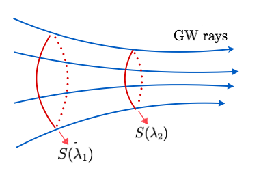
We call $S(\lambda)$ the cross-sectional area of a GW bundle, and $\lambda$ the affine parameter along each GW ray (the graviton trajectory) with four-momentum $k^{\mu}$. A geometric optics theorem (see [64], exercise 22.13) states that

$$\frac{d\,S(\lambda)}{d\lambda}-\nabla_{\mu}k^{\mu}\,S(\lambda)\,=\,0\,,$$

(34)

with $\lambda$ the affine parameter associated with the GW 4-momentum $k^{\mu}$. Together with (33), relation (34) implies the important identity

$$\frac{d}{d\lambda}\left\{e^{-\int{\cal T}}\,{\cal A}_{T}^{2}\,S\right\}\,=\,0\,,$$

(35)

that makes more manifest the required flux conservation for a stream of gravitons crossing the $S$-areas along the GW evolution parameterized with $\lambda$. Notice the presence of the overall exponential factor $e^{-\int{\cal T}}$ due to modified gravity – see the discussion after eq (25) – that changes the flux of gravitons through a given surface. Such coefficient plays the role of ‘damping term’ in the GW amplitude during propagation in a modified gravity set-up, as expected given that we interpret ${\cal T}$ as friction in the evolution equations. The result (35) will be important for cosmological applications in what follows.

To determine the GW luminosity distance we proceed step-by-step as [46]. We introduce an observer whose physical four-velocity we denote with $\hat{u}^{\mu}$. The measured GW energy flux by such observer reads

	$\displaystyle\hat{\cal F}^{\alpha}$	$\displaystyle=$	$\displaystyle-\hat{T}^{\mu}_{\,\,\nu}\,h^{\alpha}_{\,\,\mu}\,\hat{u}^{\nu}\,,$		(46)
		$\displaystyle=$	$\displaystyle{\cal F}\,\hat{n}^{\alpha}\,,$		(47)

where $\hat{T}^{\mu}_{\,\,\nu}$ is the GW energy momentum tensor (39), and

	$\displaystyle h^{\alpha}_{\,\,\mu}$	$\displaystyle=$	$\displaystyle\delta^{\alpha}_{\,\,\mu}+\hat{u}^{\alpha}\,\hat{u}_{\mu}\,,$		(48)
	$\displaystyle\hat{n}^{\alpha}$	$\displaystyle=$	$\displaystyle\frac{1}{\omega}\left(\hat{k}^{\alpha}-\omega\hat{u}^{\alpha}\right)\,,$		(49)

while the GW flux amplitude and GW frequency measured by the observer are

	$\displaystyle{\cal F}$	$\displaystyle=$	$\displaystyle\frac{e^{-\int\,{\cal T}}}{32\,\pi}\,{\cal A}_{T}^{2}\,\omega^{2}\,,$		(50)
	$\displaystyle\omega$	$\displaystyle=$	$\displaystyle-\hat{k}_{\mu}\hat{u}^{\mu}\,.$		(51)

The notion of GW frequency allows us to define the GW redshift $z$ at the value $\lambda$ of the comoving GW geodesics affine parameter $\lambda$

$$1+z(\lambda)\,=\,\frac{\omega(\lambda)}{\omega(0)}\,.$$

(52)

For computing the luminosity distance, we assume that GW are emitted by an approximately spherically symmetric system, with characteristic radius $R_{s}$ (this assumption is nevertheless not important since we send $R_{s}\to 0$ at the end of the calculation). The flux amplitude ${\cal F}$ measured at the source position is related with the intrinsic source luminosity by the relation

$${\cal F}(\lambda_{s})\,=\,\frac{{\cal L}_{GW}}{4\pi\,R_{s}^{2}}\,,$$

(53)

with $\lambda_{s}$ the conformal affine parameter at the source. See Fig 2, left panel. The luminosity distance to the source as measured by an observer located at $\lambda=0$ is defined as

$$d_{L}^{\rm(GW)}\,\equiv\,\left[\frac{{\cal L}_{GW}}{4\pi\,{\cal F}(0)}\right]^{\frac{1}{2}}\,=\,\sqrt{\frac{{\cal F}(\lambda_{s})}{{\cal F}(0)}}\,R_{s}\,.$$

(54)

Substituting relation (50), we find the following expression

$$d_{L}^{\rm(GW)}\,=\,\left(e^{-\frac{1}{2}\,\int_{0}^{\lambda_{s}}\,{\cal T}}\right)\,\frac{{\cal A}_{T}(\lambda_{s})}{{\cal A}_{T}(0)}\,\left[1+z(\lambda_{s})\right]\,R_{s}\,.$$

(55)

Notice the role of the modified gravity friction term in the overall exponential factor, containing the cumulative integral of the friction parameter ${\cal T}$ along the GW geodesics path (see the discussion after eq (25)). Before proceeding, to make contact with the literature, it is interesting to consider the ratio between the GW luminosity distance (55) versus the electromagnetic luminosity distance. This ratio provides an interesting observable in case of multimessenger events. We find

$$\frac{d_{L}^{\rm(GW)}}{d_{L}^{\rm(EM)}}\,=\,\exp{\left[-\frac{1}{2}\,\int^{\lambda_{S}}_{0}\,{\cal T}\,\frac{d\bar{\phi}}{d\lambda^{\prime}}\,d\lambda^{\prime}\right]}\,,$$

(56)

singling out the modified gravity contribution as an integral from $\lambda=0$ (the position of the observer) to the source at $\lambda=\lambda_{S}$. Once substituting in the integrand of (56) the explicit form of friction terms used for parameterizing deviations from GR in cosmological models of dark energy, one finds exactly the same formulas used in the literature – see Appendix D for a discussion of such comparison.

We now proceed expressing the GW luminosity distance (55) in an alternative way, that is more useful for explicitly including effects of cosmological perturbations, and for then comparing with the angular distance in section 4.2. From now on, we denote a a perturbed quantity with a tilde, and unperturbed without tilde. For example, we write for the comoving metric

$$\tilde{g}_{\mu\nu}\,=\,\eta_{\mu\nu}+\delta g_{\mu\nu}\,,$$

(57)

meaning that $\delta g_{\mu\nu}$ are long-wavelength perturbations. We now introduce a null vector $\tilde{K}^{\mu}$ proportional to $\tilde{k}^{\mu}$, and use it to define a corresponding affine parameterization:

$$\tilde{K}^{\mu}\,\equiv\,-\frac{\tilde{k}^{\mu}}{\tilde{\omega}(\lambda_{s})a(\tilde{\eta}(\lambda_{s}))}\,,$$

(58)

where $\lambda$ from now on is the affine parameter associated with $\tilde{K}^{\mu}$. This vector is normalized in such a way that, once evaluated at the source $\lambda=\lambda_{s}$, we find

$$\left(\tilde{g}_{\mu\nu}\tilde{K}^{\mu}\tilde{u}^{\nu}\right)_{\lambda_{s}}\,=\,1\,,$$

(59)

where $\tilde{u}^{\mu}$ is the perturbed comoving observer 4-velocity.

The introduction of the vector $\tilde{K}^{\mu}$. is technically convenient to easily relate the physical size of the source with the affine parameter along the GW geodesics. In fact, as shown in [46], the characteristic size $R_{s}$ of the source can be expressed as

$$R_{s}\,=\,a(\tilde{\eta}(\lambda_{s}))\,\Delta\lambda_{s}\,,$$

(60)

with $\Delta\lambda_{s}$ the infinitesimal affine parameter associated with the source size. See Fig 2, left panel.

If the unperturbed case, it is straightforward to integrate (43) (recalling that we have no shear for a spherically symmetric source): we get

$$\theta_{L}\,=\,\frac{2}{\lambda-\lambda_{s}-\Delta\lambda_{s}}\,,$$

(61)

where the suffix $L$ is included to associate the expansion parameter $\theta$ with the luminosity distance. The deviation for the expression of $\theta_{L}$ at first order in cosmological inhomogeneities can be expressed as

$$\delta\theta_{L}(\lambda)\,=\,\tilde{\theta}_{L}\left[x^{\mu}(\lambda)+\delta x^{\mu}(\lambda)\right]-\theta_{L}\left[x^{\mu}(\lambda)\right]\,.$$

(62)

The evolution equation for the first order perturbation $\delta\theta_{L}(\lambda)$ can be obtained from from (43). It reads

$$\frac{d\,\delta\theta_{L}}{d\lambda}\,=\,-\theta_{L}\,\delta\theta_{L}-\delta(R_{\mu\nu}K^{\mu}K^{\nu})_{\lambda}$$

(63)

where $R_{\mu\nu}$ is the perturbed space-time Ricci tensor at the position $\lambda$ along the GW geodesics. Integrating eq (63) along the affine parameter, imposing the boundary condition $\delta\theta_{L}(\lambda_{s})=0$, we get

$$\delta\theta_{L}(\lambda)\,=\,\frac{1}{(\lambda-\lambda_{s}-\Delta\lambda_{s})^{2}}\,\int_{\lambda}^{\lambda_{s}}\,d\lambda^{\prime}\,\left(\lambda^{\prime}-\lambda_{s}-\Delta\lambda_{s}\right)^{2}\,\delta(R_{\mu\nu}K^{\mu}K^{\nu})_{\lambda^{\prime}}\,\,.$$

(64)

Collecting all the results so far, we can integrate eq (42), and get the relation

$$\exp{\left[-\frac{1}{2}\,\int_{0}^{\lambda_{s}}\,{\cal T}\right]}\,\times\,\frac{{\cal A}_{T}(\lambda_{s})\,a(\tilde{\eta}(\lambda_{s}))}{{\cal A}_{T}(0)\,a(\tilde{\eta}(0))}\,=\,\frac{\lambda_{s}+\Delta\lambda_{s}}{\Delta\lambda_{s}}\,\exp{\left[-\frac{1}{2}\int_{0}^{\lambda_{s}}d\lambda\,\delta\theta_{L}(\lambda)\right]}\,\,.$$

(65)

This result can be inserted into eq (55): taking $\Delta\lambda_{s}\to 0$ (i.e. considering a source of negligible size) we end with the compact expression

$$\tilde{d}_{L}^{\rm(GW)}(\lambda_{s})\,=\,\lambda_{s}\,a[\tilde{\eta}(0)]\,\left[1+\tilde{z}(\lambda_{s})\right]\,\times\,\exp{\left[-\frac{1}{2}\int_{0}^{\lambda_{s}}d\lambda\,\delta\theta_{L}(\lambda)\right]}\,.$$

(66)

The compact expression (66) (accompanied by relation (65)) is exact and include the effects of cosmological fluctuations – on the other hand is implicitly expressed in terms of $\lambda_{s}$, and is not easy from it to extract in a physically transparent way the implications of cosmological fluctuations and of modified gravity. Such implications are more easily studied by using the cosmic ruler formalism – see [55]. This approach explicitly identifies contributions from peculiar velocities, weak lensing, Sachs-Wolfe effects, volume effects, and Shapiro time delay, and allows to appreciate the contributions due to modified gravity. We refer the reader to [55] for more details: for our purposes to prove the validity of Etherington reciprocity law – our aim for the next section – formula (66) will be sufficient.

We now prove the validity of Etherington reciprocity law connecting luminosity and angular GW distances. This relation is expected to hold in scenarios where graviton number is conserved, as our scalar-tensor set-up (see section 3.4).

The GW angular distance $d_{A}^{\rm GW}$ is formally defined in terms of the ratio between the angular diameter $d_{s}$ of the source located at conformal affine parameter $\lambda_{s}$, and the source apparent angular size $\Delta\phi$ as measured by an observer at $\lambda=0$. In formulas:

$$d_{A}^{\rm(GW)}\,=\,\frac{d_{s}}{\Delta\phi}\,.$$

(67)

Following [46], it is convenient to re-express $d_{A}^{\rm(GW)}$ as

$$d_{A}^{\rm(GW)}\,=\,\left(\frac{S(\lambda_{s})}{S(\Delta\lambda)}\right)^{1/2}\,\frac{{\bf d}(\Delta\lambda)}{\Delta\phi}\,,$$

(68)

with $S(\lambda)$ the cross-section area of GW rays at $\lambda$, and its diameter by ${\bf d}(\lambda)$. $\Delta\lambda$ is the affine parameter in proximity of the observer. [46] proved the relation

$$\frac{{\bf d}(\Delta\lambda)}{\Delta\phi}\,=\,\frac{a^{2}[\tilde{\eta}(0)]\,\Delta\lambda}{(1+\tilde{z}(\lambda_{s}))\,a[\tilde{\eta}(\lambda_{s})]}\,,$$

(69)

connecting the ratio ${{\bf d}(\Delta\lambda)}/{\Delta\phi}$ with $\Delta\lambda$. See Fig 2, right panel.

Fig 2 shows that in evaluating the angular distance one considers GW bundles expanding from the observer position (while, on the contrary, the luminosity distance considers bundles expanding from the source). Hence, the expansion parameter $\theta_{A}$ associated with angular distance reads, when neglecting effects of cosmological inhomogenities, can be obtained integrating eq (43):

$$\theta_{A}\,=\,\frac{2}{\lambda}\,.$$

(70)

When including the contributions of perturbations, we find the formal solution

$$\delta\theta_{A}\,=\,-\frac{1}{\lambda^{2}}\,\int_{0}^{\lambda}\,d\lambda^{\prime}\,\lambda^{\prime 2}\,\delta(R_{\mu\nu}K^{\mu}K^{\nu})_{\lambda}^{\prime}\,,$$

(71)

for the first order perturbation $\delta\theta_{A}$ to the angular expansion parameter.

Integrating eq (45) along the GW geodesics, and comparing with the definition (68), we get the relation

$$d_{A}^{\rm(GW)}\,=\,\exp{\left[\frac{1}{2}\,\int_{0}^{\lambda_{s}}\,{\cal T}\right]}\,\times\,\left(\frac{{\cal A}_{T}(0)}{{\cal A}_{T}(\lambda_{s})}\right)\,\times\,\frac{{\bf d}(\Delta\lambda)}{\Delta\phi}\,.$$

(72)

Moreover, integrating eq (42) using the result (70), we now obtain

$$\exp{\left[-\frac{1}{2}\,\int_{0}^{\lambda_{s}}\,{\cal T}\right]}\,\times\,\frac{{\cal A}_{T}(\lambda_{s})\,a(\tilde{\eta}(\lambda_{s}))}{{\cal A}_{T}(0)\,a(\tilde{\eta}(0))}\,=\,\frac{\Delta\lambda}{\lambda_{s}}\,\exp{\left[-\frac{1}{2}\int_{\Delta\lambda}^{\lambda_{s}}d\lambda\,\delta\theta_{A}(\lambda)\right]}$$

(73)

as the relation between affine parameter and angular expansion parameter. Substituting the results of eqs (73) and (69) into eq (72), we obtain the expression

$$\tilde{d}_{A}^{\rm(GW)}\,=\,\frac{a[\tilde{\eta}(0)]}{1+\tilde{z}(\lambda_{s})}\,\lambda_{s}\,\exp{\left[\frac{1}{2}\int_{0}^{\lambda_{s}}\,\delta\theta_{A}(\lambda)d\lambda\right]}\,.$$

(74)

Comparing with the expression for the luminosity distance, we get

	$\displaystyle\tilde{d}_{A}^{(\rm GW)}$	$\displaystyle=$	$\displaystyle\frac{\tilde{d}_{L}^{\rm(GW)}}{(1+\tilde{z})^{2}}\,\exp{\left[\frac{1}{2}\int_{0}^{\lambda_{s}}\,\left(\delta\theta_{A}(\lambda)+\delta\theta_{L}(\lambda)\right)d\lambda\right]}\,,$		(75)
		$\displaystyle=$	$\displaystyle\frac{\tilde{d}_{L}^{\rm(GW)}}{(1+\tilde{z})^{2}}\,.$		(76)

The second line, eq (76), is the desired Etherington relation, valid including first order perturbations. (The step between eq (75) and (76) requires technical calculations that we defer to Appendix E.)

Hence we proved that in the scalar-tensor framework discussed in this work, with conservation of graviton number, luminosity and angular distances for GW are connected by the classic Etherington law (76). We have seen that GW and electromagnetic luminosity distances can differ – see eq (56) – and this fact is important in case of multimessenger events. Then eq (76) tells us that the same is true for angular distances, and we can schematically write a relation analog to eq (56):

$$\frac{d_{A}^{\rm(GW)}}{d_{A}^{\rm(EM)}}\,=\,\exp{\left[-\frac{1}{2}\,\int^{\lambda_{S}}_{0}\,{\cal T}\,\frac{d\bar{\phi}}{d\lambda}\,d\lambda\right]}\,.$$

(77)

In what comes next we briefly discuss some applications of these results to GW lensing.

Strong GW lensing from large-scale structures between GW source and detector is an important phenomenon that – although not yet observed – is likely to offer new ways to probe cosmological parameters with future gravitational wave detections. For example LISA, by observing sources from high-redshift sources, will likely detect lensed events [92]. See e.g. [76, 77, 78, 79, 80, 81, 82, 83, 84, 85, 86, 87, 88, 89, 90, 119, 91, 92, 93, 94, 92, 95, 96, 97, 98, 99, 100, 101, 102, 58, 103, 50, 104, 49, 105] for works discussing this topic.

We consider strong GW lensing from point-like lenses in the geometric optics limit, valid when the GW wavelength is well shorter than the Schwarzschild radius of the lens. In this limit, we do not need to discuss interference effects that, although very interesting, go beyond the scope of this work. We focus on the specific observable associated with the time-delay that the presence of the lens induces on the propagation time of the GW from source to detector. We compare the GW time-delay induced by the presence of the lens with the electromagnetic (EM) time delay of lensed light received in a multimessenger detection.

The works [49, 50] shown conclusively that GW and EM lensed signals arrive at the same time at the detector, if both waves propagate at the same speed and are emitted at the same time. In the geometric optics limit this is expected when photons and GW travel through null geodesics, since by definition both sectors cover the minimal possible distance from source to detector. Causality arguments based on Fermat principle allow one to prove this statement in full generality. [49] also argues that the same result should be valid in any theory of gravity, to respect causality.

Said this, it is interesting to analyze the topic in an explicit modified gravity set-up, for understanding how effects of modified gravity balance so to ensure the same time delay for GW and light. This is the scope of this section. We find this topic interesting since the expression for the time-delay commonly used in the literature (see e.g. [72], as well as the recent [103] in the context of gravitational waves) explicitly contains factors depending on the angular distance $d_{A}^{\rm{(GW)}}$, which can be modified with respect to the standard case (see eq (77)). In fact, the GW time delay $\Delta t^{\rm(GW)}$ has a geometrical contribution, and a Shapiro contribution $t_{\Phi}^{\rm(GW)}$ due to the presence of inhomogeneities in the background cosmological space-time crossed by GW in their path from source to detection. We express it in the following form

$$\Delta t^{\rm(GW)}\,=\,(1+z)\,\frac{d_{OL}^{\rm(GW)}d^{\rm(GW)}_{SO}}{2\,d^{\rm(GW)}_{SL}}\,|\theta-\theta_{S}\,|^{2}+t_{\Phi}^{\rm(GW)}\,.$$

(78)

In the previous expression, $z$ is the redshift, $d_{OL}^{\rm(GW)}$ the GW angular distance as measured from the observer to the lens, $d^{\rm(GW)}_{SO}$ the same quantity measured from source to the observer, and $d^{\rm(GW)}_{SL}$ from source to lens. $t_{\Phi}^{\rm(GW)}$ is the aforementioned Shapiro contribution due to inhomogeneities. $\theta$ is the observed angular position of the source, $\theta_{S}$ the would-be angular position of the source in absence of the lens. In the electromagnetic case, the corresponding time-delay $\Delta t^{\rm(EM)}$ has exactly the same structure, changing the suffixes from GW to EM. See Appendix F for a derivation of the geometric part (the first term) of the previous formula.

In [55] we shown explicitly that the Shapiro time-delay $t_{\Phi}$ is exactly the same for GW and EM observations in a scalar-tensor framework, $t_{\Phi}^{\rm(GW)}=t_{\Phi}^{\rm(EM)}$: we refer the reader to this work for full details. However, eq (78) also contains explicitly angular distances in the first geometric term, which we dub $\Delta t_{\rm geo}$. Using eq (77) we can in fact understand how the effects of modified gravity in the geometrical time-delay $\Delta t_{\rm geo}$ compensate. We can write:

	$\displaystyle\Delta t_{\rm geo}^{\rm(GW)}$	$\displaystyle=$	$\displaystyle(1+z)\,\frac{d_{OL}^{\rm(GW)}d^{\rm(GW)}_{SO}}{2\,d^{\rm(GW)}_{SL}}\,|\theta-\theta_{S}\,|^{2}\,,$		(79)
		$\displaystyle=$	$\displaystyle\left(\frac{d_{OL}^{\rm(GW)}}{d_{OL}^{\rm(EM)}}\right)\left(\frac{d_{SO}^{\rm(GW)}}{d_{SO}^{\rm(EM)}}\right)\left(\frac{d_{SL}^{\rm(EM)}}{d_{SL}^{\rm(GW)}}\right)\,\Delta t_{\rm geo}^{\rm(EM)}\,,$
		$\displaystyle=$	$\displaystyle\left(\exp{\left[-\frac{1}{2}\int_{\lambda_{O}}^{\lambda_{L}}{\cal T}\,\frac{d\bar{\phi}}{d\lambda}\,d\lambda-\frac{1}{2}\int_{\lambda_{S}}^{\lambda_{O}}{\cal T}\,\frac{d\bar{\phi}}{d\lambda}\,d\lambda+\frac{1}{2}\int_{\lambda_{S}}^{\lambda_{L}}{\cal T}\,\frac{d\bar{\phi}}{d\lambda}\,d\lambda\right]}\right)\,\Delta t_{\rm geo}^{\rm(EM)}\,,$
		$\displaystyle=$	$\displaystyle\,\Delta t_{\rm geo}^{\rm(EM)}\,.$

To pass from the second to third line we used relation (77), while the fourth line is a simple consequence of summing the integrals in the exponent. So we find that modified gravity contributions carefully compensate, leading to the equality $\Delta t_{\rm geo}^{\rm(GW)}\,=\,\Delta t_{\rm geo}^{\rm(EM)}$. Together with the fact that the Shapiro time delay coincides in the GW and EM sector, we find that by using the expression eq (78) we are ensured that GW and EM experience the same time-delay from strong lensing in a scalar-tensor theory of gravity, as we wish to demonstrate. In particular, even if formula (78) is expressed in terms of angular distances that, when taken individually, can be different with respect to General Relativity, one finds cancelations between modified gravity coefficients that lead to the result (79).

References

- [1] B. F. Schutz, “Determining the Hubble Constant from Gravitational Wave Observations,” Nature 323 (1986) 310–311.
- [2] D. E. Holz and S. A. Hughes, “Using gravitational-wave standard sirens,” Astrophys. J. 629 (2005) 15–22, arXiv:astro-ph/0504616 [astro-ph].
- [3] N. Dalal, D. E. Holz, S. A. Hughes, and B. Jain, “Short GRB and binary black hole standard sirens as a probe of dark energy,” Phys. Rev. D74 (2006) 063006, arXiv:astro-ph/0601275 [astro-ph].
- [4] C. L. MacLeod and C. J. Hogan, “Precision of Hubble constant derived using black hole binary absolute distances and statistical redshift information,” Phys. Rev. D77 (2008) 043512, arXiv:0712.0618 [astro-ph].
- [5] S. Nissanke, D. E. Holz, S. A. Hughes, N. Dalal, and J. L. Sievers, “Exploring short gamma-ray bursts as gravitational-wave standard sirens,” Astrophys. J. 725 (2010) 496–514, arXiv:0904.1017 [astro-ph.CO].
- [6] C. Cutler and D. E. Holz, “Ultra-high precision cosmology from gravitational waves,” Phys. Rev. D80 (2009) 104009, arXiv:0906.3752 [astro-ph.CO].
- [7] LIGO Scientific, Virgo, 1M2H, Dark Energy Camera GW-E, DES, DLT40, Las Cumbres Observatory, VINROUGE, MASTER Collaboration, B. P. Abbott et al., “A gravitational-wave standard siren measurement of the Hubble constant,” Nature 551 no. 7678, (2017) 85–88, arXiv:1710.05835 [astro-ph.CO].
- [8] P. Creminelli and F. Vernizzi, “Dark Energy after GW170817 and GRB170817A,” Phys. Rev. Lett. 119 no. 25, (2017) 251302, arXiv:1710.05877 [astro-ph.CO].
- [9] J. Sakstein and B. Jain, “Implications of the Neutron Star Merger GW170817 for Cosmological Scalar-Tensor Theories,” Phys. Rev. Lett. 119 no. 25, (2017) 251303, arXiv:1710.05893 [astro-ph.CO].
- [10] J. M. Ezquiaga and M. Zumalacárregui, “Dark Energy After GW170817: Dead Ends and the Road Ahead,” Phys. Rev. Lett. 119 no. 25, (2017) 251304, arXiv:1710.05901 [astro-ph.CO].
- [11] T. Baker, E. Bellini, P. G. Ferreira, M. Lagos, J. Noller, and I. Sawicki, “Strong constraints on cosmological gravity from GW170817 and GRB 170817A,” Phys. Rev. Lett. 119 no. 25, (2017) 251301, arXiv:1710.06394 [astro-ph.CO].
- [12] L. Lombriser and A. Taylor, “Breaking a Dark Degeneracy with Gravitational Waves,” JCAP 1603 (2016) 031, arXiv:1509.08458 [astro-ph.CO].
- [13] D. Bettoni, J. M. Ezquiaga, K. Hinterbichler, and M. Zumalacárregui, “Speed of Gravitational Waves and the Fate of Scalar-Tensor Gravity,” Phys. Rev. D95 no. 8, (2017) 084029, arXiv:1608.01982 [gr-qc].
- [14] E. Belgacem, Y. Dirian, S. Foffa, and M. Maggiore, “Gravitational-wave luminosity distance in modified gravity theories,” Phys. Rev. D97 no. 10, (2018) 104066, arXiv:1712.08108 [astro-ph.CO].
- [15] C. Deffayet and K. Menou, “Probing Gravity with Spacetime Sirens,” Astrophys. J. Lett. 668 (2007) L143–L146, arXiv:0709.0003 [astro-ph].
- [16] S. F. Daniel, R. R. Caldwell, A. Cooray, and A. Melchiorri, “Large Scale Structure as a Probe of Gravitational Slip,” Phys. Rev. D77 (2008) 103513, arXiv:0802.1068 [astro-ph].
- [17] I. D. Saltas, I. Sawicki, L. Amendola, and M. Kunz, “Anisotropic Stress as a Signature of Nonstandard Propagation of Gravitational Waves,” Phys. Rev. Lett. 113 no. 19, (2014) 191101, arXiv:1406.7139 [astro-ph.CO].
- [18] I. Sawicki, I. D. Saltas, M. Motta, L. Amendola, and M. Kunz, “Nonstandard gravitational waves imply gravitational slip: On the difficulty of partially hiding new gravitational degrees of freedom,” Phys. Rev. D95 no. 8, (2017) 083520, arXiv:1612.02002 [astro-ph.CO].
- [19] L. Amendola, I. Sawicki, M. Kunz, and I. D. Saltas, “Direct detection of gravitational waves can measure the time variation of the Planck mass,” JCAP 1808 (2018) 030, arXiv:1712.08623 [astro-ph.CO].
- [20] A. Nishizawa, “Generalized framework for testing gravity with gravitational-wave propagation. I. Formulation,” Phys. Rev. D97 no. 10, (2018) 104037, arXiv:1710.04825 [gr-qc].
- [21] S. Arai and A. Nishizawa, “Generalized framework for testing gravity with gravitational-wave propagation. II. Constraints on Horndeski theory,” Phys. Rev. D97 no. 10, (2018) 104038, arXiv:1711.03776 [gr-qc].
- [22] M. Lagos, M. Fishbach, P. Landry, and D. E. Holz, “Standard sirens with a running Planck mass,” Phys. Rev. D99 no. 8, (2019) 083504, arXiv:1901.03321 [astro-ph.CO].
- [23] S. Mukherjee, B. D. Wandelt, and J. Silk, “Multimessenger tests of gravity with weakly lensed gravitational waves,” Phys. Rev. D101 no. 10, (2020) 103509, arXiv:1908.08950 [astro-ph.CO].
- [24] S. Mukherjee, B. D. Wandelt, and J. Silk, “Probing the theory of gravity with gravitational lensing of gravitational waves and galaxy surveys,” Mon. Not. Roy. Astron. Soc. 494 no. 2, (2020) 1956–1970, arXiv:1908.08951 [astro-ph.CO].
- [25] R. D’Agostino and R. C. Nunes, “Probing observational bounds on scalar-tensor theories from standard sirens,” Phys. Rev. D100 no. 4, (2019) 044041, arXiv:1907.05516 [gr-qc].
- [26] A. Vijaykumar, S. J. Kapadia, and P. Ajith, “Constraints on the time variation of the gravitational constant using gravitational wave observations of binary neutron stars,” arXiv:2003.12832 [gr-qc].
- [27] S. Mastrogiovanni, L. Haegel, C. Karathanasis, I. Magana-Hernandez, and D. A. Steer, “Gravitational wave friction in light of GW170817 and GW190521,” arXiv:2010.04047 [gr-qc].
- [28] S. Mastrogiovanni, D. Steer, and M. Barsuglia, “Probing modified gravity theories and cosmology using gravitational-waves and associated electromagnetic counterparts,” Phys. Rev. D102 no. 4, (2020) 044009, arXiv:2004.01632 [gr-qc].
- [29] A. Nishizawa and S. Arai, “Generalized framework for testing gravity with gravitational-wave propagation. III. Future prospect,” Phys. Rev. D99 no. 10, (2019) 104038, arXiv:1901.08249 [gr-qc].
- [30] T. Baker and I. Harrison, “Constraining Scalar-Tensor Modified Gravity with Gravitational Waves and Large Scale Structure Surveys,” JCAP 2101 (2021) 068, arXiv:2007.13791 [astro-ph.CO].
- [31] S. Mukherjee, T. Broadhurst, J. M. Diego, J. Silk and G. F. Smoot, “Inferring the lensing rate of LIGO-Virgo sources from the stochastic gravitational wave background,” Mon. Not. Roy. Astron. Soc. 501 (2021) no.2, 2451 arXiv:2006.03064 [astro-ph.CO].
- [32] S. Mukherjee, B. D. Wandelt and J. Silk, “Testing the general theory of relativity using gravitational wave propagation from dark standard sirens,” arXiv:2012.15316 [astro-ph.CO].
- [33] E. Belgacem, Y. Dirian, S. Foffa, E. J. Howell, M. Maggiore, and T. Regimbau, “Cosmology and dark energy from joint gravitational wave-GRB observations,” JCAP 1908 (2019) 015, arXiv:1907.01487 [astro-ph.CO].
- [34] E. Belgacem, Y. Dirian, S. Foffa, and M. Maggiore, “Nonlocal gravity. Conceptual aspects and cosmological predictions,” JCAP 1803 (2018) 002, arXiv:1712.07066 [hep-th].
- [35] W. J. Wolf and M. Lagos, “Standard Sirens as a Novel Probe of Dark Energy,” Phys. Rev. Lett. 124 no. 6, (2020) 061101, arXiv:1910.10580 [gr-qc].
- [36] J. María Ezquiaga, “Hearing gravity from the cosmos: GWTC-2 probes general relativity at cosmological scales,” arXiv:2104.05139 [astro-ph.CO].
- [37] LISA Collaboration, P. Amaro-Seoane et al., “Laser Interferometer Space Antenna,” arXiv:1702.00786 [astro-ph.IM].
- [38] N. Tamanini, C. Caprini, E. Barausse, A. Sesana, A. Klein, and A. Petiteau, “Science with the space-based interferometer eLISA. III: Probing the expansion of the Universe using gravitational wave standard sirens,” JCAP 1604 (2016) 002, arXiv:1601.07112 [astro-ph.CO].
- [39] LISA Cosmology Working Group Collaboration, E. Belgacem et al., “Testing modified gravity at cosmological distances with LISA standard sirens,” JCAP 07 (2019) 024, arXiv:1906.01593 [astro-ph.CO].
- [40] E. Barausse et al., “Prospects for Fundamental Physics with LISA,” Gen. Rel. Grav. 52 no. 8, (2020) 81, arXiv:2001.09793 [gr-qc].
- [41] M. Maggiore et al., “Science Case for the Einstein Telescope,” JCAP 2003 (2020) 050, arXiv:1912.02622 [astro-ph.CO].
- [42] P. Laguna, S. L. Larson, D. Spergel, and N. Yunes, “Integrated Sachs-Wolfe Effect for Gravitational Radiation,” Astrophys. J. 715 (2010) L12, arXiv:0905.1908 [gr-qc].
- [43] D. Bertacca, A. Raccanelli, N. Bartolo, and S. Matarrese, “Cosmological perturbation effects on gravitational-wave luminosity distance estimates,” Phys. Dark Univ. 20 (2018) 32–40, arXiv:1702.01750 [gr-qc].
- [44] J. Fier, X. Fang, B. Li, S. Mukohyama, A. Wang, and T. Zhu, “Gravitational wave cosmology I: high frequency approximation,” arXiv:2102.08968 [astro-ph.CO].
- [45] E. Belgacem, Y. Dirian, S. Foffa, and M. Maggiore, “Modified gravitational-wave propagation and standard sirens,” Phys. Rev. D98 no. 2, (2018) 023510, arXiv:1805.08731 [gr-qc].
- [46] M. Sasaki, “The Magnitude - Redshift relation in a perturbed Friedmann universe,” Mon. Not. Roy. Astron. Soc. 228 (1987) 653–669.
- [47] R. Arjona, H.-N. Lin, S. Nesseris, and L. Tang, “Machine learning forecasts of the cosmic distance duality relation with strongly lensed gravitational wave events,” arXiv:2011.02718 [astro-ph.CO].
- [48] M. Oguri, “Strong gravitational lensing of explosive transients,” Rept. Prog. Phys. 82 no. 12, (2019) 126901, arXiv:1907.06830 [astro-ph.CO].
- [49] T. Suyama, “On arrival time difference between lensed gravitational waves and light,” Astrophys. J. 896 no. 1, (2020) 46, arXiv:2003.11748 [gr-qc].
- [50] J. M. Ezquiaga, W. Hu, and M. Lagos, “Apparent Superluminality of Lensed Gravitational Waves,” Phys. Rev. D 102 no. 2, (2020) 023531, arXiv:2005.10702 [astro-ph.CO].
- [51] T. Clifton, P. G. Ferreira, A. Padilla, and C. Skordis, “Modified Gravity and Cosmology,” Phys. Rept. 513 (2012) 1–189, arXiv:1106.2476 [astro-ph.CO].
- [52] D. M. Eardley, D. L. Lee, A. P. Lightman, R. V. Wagoner, and C. M. Will, “Gravitational-wave observations as a tool for testing relativistic gravity,” Phys. Rev. Lett. 30 (1973) 884–886.
- [53] D. M. Eardley, D. L. Lee, and A. P. Lightman, “Gravitational-wave observations as a tool for testing relativistic gravity,” Phys. Rev. D8 (1973) 3308–3321.
- [54] C. Dalang, P. Fleury, and L. Lombriser, “Horndeski gravity and standard sirens,” Phys. Rev. D 102 no. 4, (2020) 044036, arXiv:1912.06117 [gr-qc].
- [55] A. Garoffolo, G. Tasinato, C. Carbone, D. Bertacca, and S. Matarrese, “Gravitational waves and geometrical optics in scalar-tensor theories,” arXiv:1912.08093 [gr-qc].
- [56] A. Garoffolo, M. Raveri, A. Silvestri, G. Tasinato, C. Carbone, D. Bertacca, and S. Matarrese, “Detecting Dark Energy Fluctuations with Gravitational Waves,” arXiv:2007.13722 [astro-ph.CO].
- [57] C. Dalang, P. Fleury, and L. Lombriser, “Scalar and tensor gravitational waves,” arXiv:2009.11827 [gr-qc].
- [58] J. M. Ezquiaga and M. Zumalacárregui, “Gravitational wave lensing beyond general relativity: birefringence, echoes and shadows,” arXiv:2009.12187 [gr-qc].
- [59] C. Cheung, P. Creminelli, A. L. Fitzpatrick, J. Kaplan, and L. Senatore, “The Effective Field Theory of Inflation,” JHEP 03 (2008) 014, arXiv:0709.0293 [hep-th].
- [60] G. Gubitosi, F. Piazza, and F. Vernizzi, “The Effective Field Theory of Dark Energy,” JCAP 1302 (2013) 032, arXiv:1210.0201 [hep-th]. [JCAP1302,032(2013)].
- [61] F. Piazza and F. Vernizzi, “Effective Field Theory of Cosmological Perturbations,” Class. Quant. Grav. 30 (2013) 214007, arXiv:1307.4350 [hep-th].
- [62] R. A. Isaacson, “Gravitational Radiation in the Limit of High Frequency. I. The Linear Approximation and Geometrical Optics,” Phys. Rev. 166 (1968) 1263–1271.
- [63] R. A. Isaacson, “Gravitational Radiation in the Limit of High Frequency. II. Nonlinear Terms and the Ef fective Stress Tensor,” Phys. Rev. 166 (1968) 1272–1279.
- [64] C. W. Misner, K. S. Thorne, and J. A. Wheeler, Gravitation. W. H. Freeman, San Francisco, 1973.
- [65] M. Maggiore, Gravitational Waves. Vol. 1: Theory and Experiments. Oxford Master Series in Physics. Oxford University Press, 2007. http://www.oup.com/uk/catalogue/?ci=9780198570745.
- [66] G. Tasinato, “Symmetries for scalarless scalar theories,” Phys. Rev. D102 no. 8, (2020) 084009, arXiv:2009.02157 [hep-th].
- [67] LIGO Scientific, Virgo Collaboration, B. P. Abbott et al., “Tests of General Relativity with GW170817,” Phys. Rev. Lett. 123 no. 1, (2019) 011102, arXiv:1811.00364 [gr-qc].
- [68] J. M. Ezquiaga and M. Zumalacárregui, “Dark Energy in light of Multi-Messenger Gravitational-Wave astronomy,” Front. Astron. Space Sci. 5 (2018) 44, arXiv:1807.09241 [astro-ph.CO].
- [69] K. Pardo, M. Fishbach, D. E. Holz, and D. N. Spergel, “Limits on the number of spacetime dimensions from GW170817,” JCAP 1807 (2018) 048, arXiv:1801.08160 [gr-qc].
- [70] G. Calcagni, S. Kuroyanagi, S. Marsat, M. Sakellariadou, N. Tamanini, and G. Tasinato, “Gravitational-wave luminosity distance in quantum gravity,” Phys. Lett. B798 (2019) 135000, arXiv:1904.00384 [gr-qc].
- [71] G. Calcagni, S. Kuroyanagi, S. Marsat, M. Sakellariadou, N. Tamanini, and G. Tasinato, “Quantum gravity and gravitational-wave astronomy,” JCAP 1910 (2019) 012, arXiv:1907.02489 [gr-qc].
- [72] P. Schneider, J. Ehlers, and E. Falco, Gravitational Lenses. Springer, 1992.
- [73] D. W. Hogg, “Distance measures in cosmology,” arXiv:astro-ph/9905116.
- [74] H. Chen, “Distance measures in gravitational-wave astrophysics and cosmology,” Class. Quant. Grav. 38 (2021) 055010, arXiv:astro-ph.CO/1709.08079 [astro-ph].
- [75] J. Baker et al., “High angular resolution gravitational wave astronomy,” arXiv:1908.11410 [astro-ph.HE].
- [76] E. L. Turner, “Gravitational lensing limits on the cosmological constant in a flat universe,” Astrophys. J. Lett. 365 (1990) L43.
- [77] Y. Wang, A. Stebbins, and E. L. Turner, “Gravitational lensing of gravitational waves from merging neutron star binaries,” Phys. Rev. Lett. 77 (1996) 2875–2878, arXiv:astro-ph/9605140 [astro-ph].
- [78] T. T. Nakamura, “Gravitational lensing of gravitational waves from inspiraling binaries by a point mass lens,” Phys. Rev. Lett. 80 (1998) 1138–1141.
- [79] Y. Wang, “Analytical modeling of the weak lensing of standard candles,” Astrophys. J. 525 (1999) 651, arXiv:astro-ph/9901212 [astro-ph].
- [80] J.-P. Macquart, “Scattering of gravitational radiation: Second order moments of the wave amplitude,” Astron. Astrophys. 422 (2004) 761–775, arXiv:astro-ph/0402661 [astro-ph].
- [81] R. Takahashi and T. Nakamura, “Wave effects in gravitational lensing of gravitational waves from chirping binaries,” Astrophys. J. 595 (2003) 1039–1051, arXiv:astro-ph/0305055 [astro-ph].
- [82] N. Seto, “Strong gravitational lensing and localization of merging massive black hole binaries with LISA,” Phys. Rev. D69 (2004) 022002, arXiv:astro-ph/0305605 [astro-ph].
- [83] C.-M. Yoo, K.-i. Nakao, H. Kozaki, and R. Takahashi, “Lensing effects on gravitational waves in a clumpy universe: effects of inhomogeneity on the distance-redshift relation,” Astrophys. J. 655 (2007) 691–703, arXiv:astro-ph/0604123 [astro-ph].
- [84] N. Seto, “Demagnified GWs from Cosmological Double Neutron Stars and GW Foreground Cleaning Around 1Hz,” Phys. Rev. D80 (2009) 103001, arXiv:0910.4812 [gr-qc].
- [85] C. Shapiro, D. Bacon, M. Hendry, and B. Hoyle, “Delensing Gravitational Wave Standard Sirens with Shear and Flexion Maps,” Mon. Not. Roy. Astron. Soc. 404 (2010) 858–866, arXiv:0907.3635 [astro-ph.CO].
- [86] M. Sereno, A. Sesana, A. Bleuler, P. Jetzer, M. Volonteri, and M. C. Begelman, “Strong lensing of gravitational waves as seen by LISA,” Phys. Rev. Lett. 105 (2010) 251101, arXiv:1011.5238 [astro-ph.CO].
- [87] C. Van Den Broeck, M. Trias, B. S. Sathyaprakash, and A. M. Sintes, “Weak lensing effects in the measurement of the dark energy equation of state with LISA,” Phys. Rev. D81 (2010) 124031, arXiv:1001.3099 [gr-qc].
- [88] M. Sereno, P. Jetzer, A. Sesana, and M. Volonteri, “Cosmography with strong lensing of LISA gravitational wave sources,” Mon. Not. Roy. Astron. Soc. 415 (2011) 2773, arXiv:1104.1977 [astro-ph.CO].
- [89] T. Baker and M. Trodden, “Multimessenger time delays from lensed gravitational waves,” Phys. Rev. D95 no. 6, (2017) 063512, arXiv:1612.02004 [astro-ph.CO].
- [90] K. Kyutoku and N. Seto, “Gravitational-wave cosmography with LISA and the Hubble tension,” Phys. Rev. D95 no. 8, (2017) 083525, arXiv:1609.07142 [astro-ph.CO].
- [91] L. Dai and T. Venumadhav, “On the waveforms of gravitationally lensed gravitational waves,” arXiv:1702.04724 [gr-qc].
- [92] M. Oguri, “Effect of gravitational lensing on the distribution of gravitational waves from distant binary black hole mergers,” Mon. Not. Roy. Astron. Soc. 480 no. 3, (2018) 3842–3855, arXiv:1807.02584 [astro-ph.CO].
- [93] L. Dai, S.-S. Li, B. Zackay, S. Mao, and Y. Lu, “Detecting Lensing-Induced Diffraction in Astrophysical Gravitational Waves,” Phys. Rev. D98 no. 10, (2018) 104029, arXiv:1810.00003 [gr-qc].
- [94] K. Haris, A. K. Mehta, S. Kumar, T. Venumadhav, and P. Ajith, “Identifying strongly lensed gravitational wave signals from binary black hole mergers,” arXiv:1807.07062 [gr-qc].
- [95] S. Hou, X.-L. Fan, K. Liao, and Z.-H. Zhu, “Gravitational Wave Interference via Gravitational Lensing: Measurements of Luminosity Distance, Lens Mass, and Cosmological Parameters,” Phys. Rev. D101 no. 6, (2020) 064011, arXiv:1911.02798 [gr-qc].
- [96] B. Liu, Z. Li, and Z.-H. Zhu, “Complementary constraints on dark energy equation of state from strongly lensed gravitational wave,” Mon. Not. Roy. Astron. Soc. 487 no. 2, (2019) 1980–1985, arXiv:1904.11751 [astro-ph.CO].
- [97] A. K. Meena and J. S. Bagla, “Gravitational lensing of gravitational waves: wave nature and prospects for detection,” Mon. Not. Roy. Astron. Soc. 492 no. 1, (2020) 1127–1134, arXiv:1903.11809 [astro-ph.CO].
- [98] O. A. Hannuksela, K. Haris, K. K. Y. Ng, S. Kumar, A. K. Mehta, D. Keitel, T. G. F. Li, and P. Ajith, “Search for gravitational lensing signatures in LIGO-Virgo binary black hole events,” Astrophys. J. Lett. 874 no. 1, (2019) L2, arXiv:1901.02674 [gr-qc].
- [99] T. Morita and J. Soda, “Arrival Time Differences of Lensed Massive Gravitational Waves,” arXiv:1911.07435 [gr-qc].
- [100] G. Cusin and N. Tamanini, “Characterisation of lensing selection effects for LISA massive black hole binary mergers,” arXiv:2011.15109 [astro-ph.CO].
- [101] P. T. H. Pang, O. A. Hannuksela, T. Dietrich, G. Pagano, and I. W. Harry, “Lensed or not lensed: Determining lensing magnifications for binary neutron star mergers from a single detection,” arXiv:2002.04893 [astro-ph.HE].
- [102] D. Rubin, I. Szapudi, B. J. Shappee, and G. S. Anand, “Does Gravity Fall Down? Evidence for Gravitational-wave Deflection along the Line of Sight to GW170817,” Astrophys. J. Lett. 890 no. 1, (2020) L6, arXiv:2001.01710 [astro-ph.CO].
- [103] J. M. Ezquiaga, D. E. Holz, W. Hu, M. Lagos, and R. M. Wald, “Phase effects from strong gravitational lensing of gravitational waves,” arXiv:2008.12814 [gr-qc].
- [104] R. Takahashi, “Arrival time differences between gravitational waves and electromagnetic signals due to gravitational lensing,” Astrophys. J. 835 no. 1, (2017) 103, arXiv:1606.00458 [astro-ph.CO].
- [105] O. Contigiani, “Lensing efficiency for gravitational wave mergers,” Mon. Not. Roy. Astron. Soc. 492 no. 3, (2020) 3359–3363, arXiv:2001.01135 [astro-ph.CO].
- [106] I. Etherington, “Republication of: LX. On the definition of distance in general relativity,” Gen. Relativ. Gravit. 39 (2007) 1055.
- [107] T. Pyne and M. Birkinshaw, “The luminosity distance in perturbed flrw spacetimes,” Mon. Not. Roy. Astron. Soc. 348 (2004) 581, arXiv:astro-ph/0310841 [astro-ph].
- [108] D. E. Holz and E. V. Linder, “Safety in numbers: Gravitational lensing degradation of the luminosity distance-redshift relation,” Astrophys. J. 631 (2005) 678–688, arXiv:astro-ph/0412173 [astro-ph].
- [109] C. Bonvin, R. Durrer, and M. A. Gasparini, “Fluctuations of the luminosity distance,” Phys. Rev. D73 (2006) 023523, arXiv:astro-ph/0511183 [astro-ph]. [Erratum: Phys. Rev.D85,029901(2012)].
- [110] L. Hui and P. B. Greene, “Correlated Fluctuations in Luminosity Distance and the (Surprising) Importance of Peculiar Motion in Supernova Surveys,” Phys. Rev. D73 (2006) 123526, arXiv:astro-ph/0512159 [astro-ph].
- [111] R. M. Wald, General Relativity. Chicago Univ. Pr., Chicago, USA, 1984.
- [112] B. A. Bassett and M. Kunz, “Cosmic distance-duality as a probe of exotic physics and acceleration,” Phys. Rev. D 69 (2004) 101305, arXiv:astro-ph/0312443.
- [113] C. Brans and R. H. Dicke, “Mach’s principle and a relativistic theory of gravitation,” Phys. Rev. 124 (1961) 925–935. [,142(1961)].
- [114] G. W. Horndeski, “Second-order scalar-tensor field equations in a four-dimensional space,” Int. J. Theor. Phys. 10 (1974) 363–384.
- [115] J. Gleyzes, D. Langlois, F. Piazza, and F. Vernizzi, “Healthy theories beyond Horndeski,” Phys. Rev. Lett. 114 no. 21, (2015) 211101, arXiv:1404.6495 [hep-th].
- [116] D. Langlois and K. Noui, “Degenerate higher derivative theories beyond Horndeski: evading the Ostrogradski instability,” JCAP 1602 (2016) 034, arXiv:1510.06930 [gr-qc].
- [117] M. Crisostomi, K. Koyama, and G. Tasinato, “Extended Scalar-Tensor Theories of Gravity,” JCAP 1604 no. 04, (2016) 044, arXiv:1602.03119 [hep-th].
- [118] J. Ben Achour, M. Crisostomi, K. Koyama, D. Langlois, K. Noui, and G. Tasinato, “Degenerate higher order scalar-tensor theories beyond Horndeski up to cubic order,” JHEP 12 (2016) 100, arXiv:1608.08135 [hep-th].
- [119] T. E. Collett and D. Bacon, “Testing the speed of gravitational waves over cosmological distances with strong gravitational lensing,” Phys. Rev. Lett. 118 no. 9, (2017) 091101, arXiv:1602.05882 [astro-ph.HE].