跳到论文正文
W Papers独立论文阅读器 arXiv:2102.13625 论文正文 计算阅读时间 · 0%
引用这篇论文根据当前论文元数据生成,正式投稿前建议核对。


License: arXiv.org perpetual non-exclusive license
arXiv:2102.13625v1 [stat.ML] 26 Feb 2021
 

Learning Prediction Intervals for Regression: Generalization and Calibration


Haoxian Chen          Ziyi Huang          Henry Lam          Huajie Qian          Haofeng Zhang

IEOR Columbia University          EE Columbia University          IEOR Columbia University          Alibaba Group          IEOR Columbia University

Abstract

We study the generation of prediction intervals in regression for uncertainty quantification. This task can be formalized as an empirical constrained optimization problem that minimizes the average interval width while maintaining the coverage accuracy across data. We strengthen the existing literature by studying two aspects of this empirical optimization. First is a general learning theory to characterize the optimality-feasibility tradeoff that encompasses Lipschitz continuity and VC-subgraph classes, which are exemplified in regression trees and neural networks. Second is a calibration machinery and the corresponding statistical theory to optimally select the regularization parameter that manages this tradeoff, which bypasses the overfitting issues in previous approaches in coverage attainment. We empirically demonstrate the strengths of our interval generation and calibration algorithms in terms of testing performances compared to existing benchmarks.

1 Introduction

While most literature in machine learning focuses on point prediction, uncertainty quantification plays, arguably, an equally important role in reliability assessment and risk-based decision-making. In regression, a natural approach to quantify uncertainty is the prediction interval (PI), namely an upper and lower limit for a given feature value XX that covers the corresponding outcome YY with high probability. The interval center represents the expected outcome, whereas the width represents the uncertainty. A test point with a high expected outcome, but wide PI width, means that the outcome can still be low with a significant chance, thus signifies a downside risk that should not be overlooked.

In this paper, we study the construction of PIs that satisfy an overall target prediction level across data, known as the expected coverage rate (Rosenfeld et al. 2018). Compared to widely used conditional (on XX) coverage rate, this notion is advantageously more tangible to measure and easier to achieve. This means that a much wider class of models can be trained to build PIs, as less conditions are needed to impose on the true relation and the model class to obtain satisfactory guarantees. In general, constructing a good PI in this framework requires balancing a tradeoff between the expected interval width and coverage maintenance, which can be formalized as an empirical constrained optimization. This viewpoint has been used in Khosravi et al. 2010 and Pearce et al. 2018 that focus on neural networks, Rosenfeld et al. 2018 that studies a dual formulation, and Galván et al. 2017 that uses multi-objective evolutionary optimization. It also relates to the learning of minimum volume sets (Polonik 1997; Scott and Nowak 2006) in which a similar tradeoff between volume and probability content appears. Building on these works, our goal in this paper is to study two key inter-related statistical aspects of this empirical constrained optimization that enhances previous results both in theory and in practice:

Feasibility-Optimality Tradeoff for Interval Models. We develop a learning theory for the PIs constructed from empirical constrained optimization that statistically achieves both feasibility (coverage) and optimality (interval width). Methodologically, we build a general “sensitivity measure” that controls this tradeoff, which in turn requires developing deviation bounds for simultaneous empirical processes. Our theory in particular covers the Lipschitz continuous model class (in parameter) and finite Vapnik–Chervonenkis (VC)-subgraph class, exemplified by a wide class of neural networks and regression trees. Such type of joint coverage-width learning guarantees appears the first in the literature. It expands the coverage-only results and the considered model classes in Rosenfeld et al. 2018. It also generalizes Scott and Nowak 2006 as both our constraints and objectives possess extra sophistication related to the shape requirement of the set as an interval, and also we characterize feasibility and optimality attainments explicitly instead of the implicit metric in Scott and Nowak 2006.

Calibration Method and Performance Guarantees. We propose a general-purpose, ready-to-implement calibration methodology to guarantee overall PI coverage with prefixed confidence. This approach is guided by a novel utilization of the high-dimensional Berry-Esseen theorem (Chernozhukov et al. 2017). It is designed to combat the overfitting issue of interval models and perform accurately on the test set. We demonstrate empirically how our approach either outperforms other methods in terms of achieving correct coverages or, for those methods with comparable coverages, we attain shorter interval widths. Moreover, our approach applies, with little adjustment, to accurately construct multiple PIs at different prediction levels simultaneously. This adds extra flexibility for decision-makers to construct PIs without needing to pre-select the prediction level in advance.

2 Related Work

We first review two most closely related methods, and then move on to other works.

Conformal Learning (CL). First proposed in Vovk et al. 2005, conformal learning (CL) is a class of methods that leverage data exchangeability to constructs PIs with finite-sample and distribution-free coverage guarantees. The original CL requires retraining for each possible test point and is therefore computationally prohibitive in general. Split/inductive CL (Papadopoulos 2008; Lei et al. 2015; Lei et al. 2018) improves the computational efficiency based on a holdout validation that avoids retraining, but at the cost of higher variability and wider intervals due to less efficient data use. Lying in between are variants based on more efficient cross-validation schemes, including leave-one-out (or the Jackknife; Barber et al. 2019; Alaa and van der Schaar 2020; Steinberger and Leeb 2016), K-fold (Vovk 2015) and ensemble methods (Gupta et al. 2019; Kim et al. 2020). Recently, quantile regression are combined with CL (Kivaranovic et al. 2020; Romano et al. 2019) to take into account the heterogeneity of uncertainties across feature values. Despite its generality, the coverage guarantees from CL are only marginal with respect to the training data (except split CL (Vovk 2012)), whereas our proposed calibration method provides a stronger high confidence guarantee. Moreover, our approach explicitly optimizes the interval width, therefore typically generates shorter PIs than CL.

Quantile Regression (QR). Quantile regression (QR) estimates the conditional quantiles of YY that can be used to construct PIs. Classical QR methods require strong assumptions (e.g., linearity or other parametric forms; Chapter 4 in Koenker and Hallock 2001). Approaches that relax these assumptions include quantile regression forests (QRF) (Meinshausen 2006) and kernel support vector machine (SVM) (Steinwart et al. 2011). However, little is known about their finite-sample coverage performance because of estimation errors in the quantiles. Recently, Kivaranovic et al. 2020 proposes calibrating the weight parameter in the pinball loss on a holdout data set to enhance PI coverage. This calibration scheme, however, does not address overfitting on the holdout set, thus could fall short of providing correct coverages on test data as our experiments show.

Other Approaches. PI construction has been substantially studied in classical statistics. To understand this construction, the error of a (point) prediction can typically be decomposed into two components: model uncertainty, which comes from the variability in the training data or method, and outcome uncertainty, which comes from the noise of YY conditional on XX. The classical literature often assumes well-defined and simple forms on the relation between XX and YY (e.g., linear model, Gaussian; Seber and Lee 2012). In this case, model uncertainty reduces to parameter estimation errors. Outcome uncertainty, on the other hand, is intrinsic in the population distribution but not the training, i.e. it arises even if the model is perfectly trained. An array of methods account for both sources of variability, which utilize approaches ranging from asymptotic normality (Seber and Lee 2012), deconvolution (Schmoyer 1992), and resampling schemes such as the bootstrap (Stine 1985) and jackknife (Steinberger and Leeb 2016).

To overcome the strong assumptions in classical statistical models, several model-free approaches have been developed. Nonparametric regression, such as spline or kernel-based methods (Doksum and Koo 2000; Olive 2007), removes rigid model assumptions but at the expense of strong dimension dependence. Gaussian processes or kriging-based methods (Sacks et al. 1989), popular in the areas of metamodeling and computer emulation, regard outcomes as a response surface and perform Gaussian posterior updates. In particular, stochastic kriging (SK) model (Ankenman et al. 2010) constructs PIs that account for both model and output variabilities by using a prior correlation structure that entails both. However, SK does not deliver a frequentist coverage guarantee nor convergence rate. More recently, uncertainty quantification of neural networks regarding their model and output variabilities are studied, via methods such as the delta method and the bootstrap (Papadopoulos et al. 2001; Khosravi et al. 2011). Nonetheless, like in classical statistical models, these approaches can only capture variability due to data and training noises, but not the bias against the true relation.

Lastly, our PI construction follows the high-quality criterion in works including Khosravi et al. 2010; Khosravi et al. 2011; Galván et al. 2017; Pearce et al. 2018; Rosenfeld et al. 2018; Zhang et al. 2019; Zhu et al. 2019, which propose various loss functions to capture the width-coverage tradeoff. They are also related to the highest density intervals in statistics (Box and Tiao 2011). Our investigations in this paper provide theoretical guarantees in using this criterion.

3 PI Learning as Empirical Constrained Optimization

We consider the general regression setting where X∈𝒳⊂ℝdX\in\mathcal{X}\subset\mathbb{R}^{d} is the feature vector and Y∈𝒴⊂ℝY\in\mathcal{Y}\subset\mathbb{R} is the outcome. Given an i.i.d. data set 𝒟:={(Xi,Yi)}i=1,…,n\mathcal{D}:=\{(X_{i},Y_{i})\}_{i=1,\ldots,n} each drawn from an unknown joint distribution π\pi, our goal is to find a PI defined as:

Definition 3.1.

An interval [L⁡(x),U⁡(x)][L(x),U(x)], where both L,U:𝒳→ℝL,U:\mathcal{X}\to\mathbb{R}, is called a prediction interval (PI) with (overall) coverage rate 1−α1-\alpha (0≤α≤10\leq\alpha\leq 1) if ℙπ​(Y∈[L⁡(X),U⁡(X)])≥1−α\mathbb{P}_{\pi}(Y\in[L(X),U(X)])\geq 1-\alpha, where ℙπ\mathbb{P}_{\pi} denotes the probability with respect to the joint distribution π\pi.

We aim to find two functions LL and UU, both in a hypothesis class ℋ\mathcal{H}. To learn the optimal high-quality PI that attains a given coverage rate 1−α1-\alpha, we consider the following constrained optimization problem:

minL,U∈ℋ​and​L≤U\displaystyle\min_{L,U\in\mathcal{H}\;\text{and}\;L\leq U} 𝔼πX​[U⁡(X)−L⁡(X)]\displaystyle\mathbb{E}_{\pi_{X}}[U(X)-L(X)] (3.1)
subject to\displaystyle\text{subject to } ℙπ​(Y∈[L⁡(X),U⁡(X)])≥1−α\displaystyle\mathbb{P}_{\pi}(Y\in[L(X),U(X)])\geq 1-\alpha

where 𝔼πX\mathbb{E}_{\pi_{X}} denotes the expectation with respect to the marginal distribution of XX. Given the data 𝒟\mathcal{D}, we approximate (3.1) with the following empirical constrained optimization problem

opt^​(t):minL,U∈ℋ​and​L≤U\displaystyle\widehat{\mathrm{opt}}(t):\min_{L,U\in\mathcal{H}\;\text{and}\;L\leq U} 𝔼π^X​[U⁡(X)−L⁡(X)]\displaystyle\mathbb{E}_{\hat{\pi}_{X}}[U(X)-L(X)] (3.2)
subject to\displaystyle\text{subject to } ℙπ^​(Y∈[L⁡(X),U⁡(X)])≥1−α+t\displaystyle\mathbb{P}_{\hat{\pi}}(Y\in[L(X),U(X)])\geq 1-\alpha+t

parameterized by t∈[0,α]t\in[0,\alpha], where 𝔼π^X\mathbb{E}_{\hat{\pi}_{X}}, ℙπ^\mathbb{P}_{\hat{\pi}} are expectation and probability with respect to the empirical distribution constructed from the data 𝒟\mathcal{D}, e.g., 𝔼π^X​[U⁡(X)−L⁡(X)]=1n​∑i=1n(U⁡(Xi)−L⁡(Xi))\mathbb{E}_{\hat{\pi}_{X}}[U(X)-L(X)]=\frac{1}{n}\sum_{i=1}^{n}(U(X_{i})-L(X_{i})). The adjustment tt, which can be viewed as a penalty term for the empirical coverage rate, is used to boost the generalized coverage performance for the optimal interval solved from opt^​(t)\widehat{\mathrm{opt}}(t): If no adjustment is made in the constraint (t=0t=0), then, because of noise, the true coverage can be lower than 1−α1-\alpha with significant probability even if the empirical coverage is above 1−α1-\alpha. A positive tt decreases the probability of such an event. Choosing tt too large, however, would eliminate more intervals from the feasible set, leading to a deterioration in the obtained expected width (objective). One of our main investigations is to balance the coverage and width performance by judiciously choosing tt.

We point out that, while our focus is on training LL and UU directly, our approach can also be applied naturally when we are given in advance a well-trained point predictor f:𝒳→ℝf:\mathcal{X}\to\mathbb{R} (obtained by any means independent of 𝒟\mathcal{D}). In this case we may seek two non-negative functions δi:𝒳→[0,∞)\delta_{i}:\mathcal{X}\to[0,\infty) such that [L⁡(x),U⁡(x)]=[f⁡(x)−δ1​(x),f⁡(x)+δ2​(x)][L(x),U(x)]=[f(x)-\delta_{1}(x),f(x)+\delta_{2}(x)]. Our subsequent development applies by constructing lower and upper bounds for the “translational” data set 𝒟~:={(Xi,Yi−f⁡(Xi))}i=1,…,n\tilde{\mathcal{D}}:=\{(X_{i},Y_{i}-f(X_{i}))\}_{i=1,\ldots,n}.

4 Joint Coverage-Width Learning Guarantees

We establish finite-sample generalization error bounds for two major classes: 1) finite VC dimensions, and 2) Lipschitz continuous in parameters, by building on a unified “sensitivity bound” on the oracle optimization. Corresponding results on consistency are provided in Appendix A. To begin, let Rt∗​(ℋ)R^{*}_{t}(\mathcal{H}) be the optimal value of

opt⁡(t):minL,U∈ℋ​and​L≤U\displaystyle\mathrm{opt}(t):\min_{L,U\in\mathcal{H}\;\text{and}\;L\leq U} 𝔼πX​[U⁡(X)−L⁡(X)]\displaystyle\mathbb{E}_{\pi_{X}}[U(X)-L(X)] (4.1)
subject to\displaystyle\text{subject to } ℙπ​(Y∈[L⁡(X),U⁡(X)])≥1−α+t\displaystyle\mathbb{P}_{\pi}(Y\in[L(X),U(X)])\geq 1-\alpha+t

which is (3.1) but with a higher target prediction level, and correspondingly R∗​(ℋ)R^{*}(\mathcal{H}) be the optimal value of (3.1). We make the following assumptions on the hypothesis class ℋ\mathcal{H}, and the conditional distribution of YY given XX:

Assumption 1.

For every function h∈ℋh\in\mathcal{H}, we have h+c∈ℋh+c\in\mathcal{H} for every constant c∈ℝc\in\mathbb{R}.

Assumption 2.

The conditional distribution of YY given X=xX=x has a density p(⋅|x)p(\cdot|x) for every x∈𝒳x\in\mathcal{X}. Moreover, for every x,yx,y such that ℙπ​(Y≤y|X=x)∈(0,1)\mathbb{P}_{\pi}(Y\leq y|X=x)\in(0,1), we have p⁡(y|x)>0p(y|x)>0 and that p(⋅|x)p(\cdot|x) is continuous at yy.

The simple closedness property in Assumption 1 turns out to allow sufficiently tight and tractable analysis for many, potentially complicated, function classes under the same roadmap. Many common classes (e.g., linear, piece-wise constant such as tree-based models, and neural networks with linear activation in the output unit) satisfy Assumption 1. It is also straightforward to enforce a class to satisfy Assumption 1 by simply adding one extra parameter. Assumption 2 is a mild non-degeneracy condition on the conditional distribution (e.g., Assumption 2 holds when p(⋅|x)p(\cdot|x) is Gaussian or uniform over a certain interval for each xx).

We have the following upper bound for Rt∗​(ℋ)−R∗​(ℋ)R^{*}_{t}(\mathcal{H})-R^{*}(\mathcal{H}) for 0<t<α0<t<\alpha:

Theorem 4.1 (Sensitivity bound with respect to target prediction level).

Suppose Assumptions 1-2 hold. For every x∈𝒳x\in\mathcal{X} and β∈(0,1)\beta\in(0,1), let Γ⁡(x,β):=inf{p⁡(y1|x)+p⁡(y2|x):ℙπ​(y1≤Y≤y2|X=x)≤1−β}\Gamma(x,\beta):=\inf\big\{p(y_{1}|x)+p(y_{2}|x):\ \mathbb{P}_{\pi}(y_{1}\leq Y\leq y_{2}|X=x)\leq 1-\beta\big\} and γβ:=sup{z>0:ℙπX​(Γ⁡(X,β)<z)≤β}\gamma_{\beta}:=\sup\{z>0:\mathbb{P}_{\pi_{X}}(\Gamma(X,\beta)<z)\leq\beta\}. Then, for every α∈(0,1)\alpha\in(0,1) and t∈(0,α)t\in(0,\alpha), we have Rt∗​(ℋ)−R∗​(ℋ)≤6​t/((α−t)​γ(α−t)/3)R^{*}_{t}(\mathcal{H})-R^{*}(\mathcal{H})\leq 6t/((\alpha-t)\gamma_{(\alpha-t)/3}).

We briefly explain how Theorem 4.1 helps develop generalization guarantees. Let ℋt2,ℋ^t2⊂ℋ2:=ℋ×ℋ\mathcal{H}^{2}_{t},\hat{\mathcal{H}}^{2}_{t}\subset\mathcal{H}^{2}:=\mathcal{H}\times\mathcal{H} be the feasible set of opt⁡(t)\mathrm{opt}(t) and opt^​(t)\widehat{\mathrm{opt}}(t) respectively. If a uniform error bound Δ​t\Delta t over the class ℋ2\mathcal{H}^{2} can be established for the empirical coverage constraint in (3.2), then ℋt+Δ​t2⊂ℋ^t2\mathcal{H}^{2}_{t+\Delta t}\subset\hat{\mathcal{H}}^{2}_{t}, therefore the shortest interval we can potentially learn from opt^​(t)\widehat{\mathrm{opt}}(t) can only be wider than the oracle optimum from (3.1) by at most Rt+Δ​t∗​(ℋ)−R∗​(ℋ)R^{*}_{t+\Delta t}(\mathcal{H})-R^{*}(\mathcal{H}). The density lower bounds in Theorem 4.1 ensure a sufficient increase of the coverage probability as interval width increases, which inversely constrains the growth of interval width as the required coverage increases.

To derive finite-sample convergence rate, we first assume the availability of certain deviation bounds for the empirical coverage rate and interval width that appear in opt^​(t)\widehat{\mathrm{opt}}(t):

Theorem 4.2 (Rate of convergence).

Suppose Assumptions 1-2 hold, and the following deviation bounds hold for every ϵ,t>0\epsilon,t>0: ℙ⁡(suph∈ℋ|𝔼π^X​[h⁡(X)]−𝔼πX​[h⁡(X)]|>ϵ)≤ϕ1​(n,ϵ,ℋ)\mathbb{P}\big(\sup_{h\in\mathcal{H}}\lvert\mathbb{E}_{\hat{\pi}_{X}}[h(X)]-\mathbb{E}_{\pi_{X}}[h(X)]\rvert>\epsilon\big)\leq\phi_{1}(n,\epsilon,\mathcal{H}) and ℙ⁡(supL,U∈ℋ​and​L≤U|ℙπ^​(Y∈[L⁡(X),U⁡(X)])−ℙπ​(Y∈[L⁡(X),U⁡(X)])|>t)≤ϕ2​(n,t,ℋ)\mathbb{P}\big(\sup_{L,U\in\mathcal{H}\;\text{and}\;L\leq U}\lvert\mathbb{P}_{\hat{\pi}}(Y\in[L(X),U(X)])-\mathbb{P}_{\pi}(Y\in[L(X),U(X)])\rvert>t\big)\leq\phi_{2}(n,t,\mathcal{H}). Then for every t∈(0,α2)t\in(0,\frac{\alpha}{2}) and ϵ>0\epsilon>0, with probability at least 1−ϕ1​(n,ϵ,ℋ)−ϕ2​(n,t,ℋ)1-\phi_{1}(n,\epsilon,\mathcal{H})-\phi_{2}(n,t,\mathcal{H}), we have, for every optimal solution (L^t∗,U^t∗)(\hat{L}_{t}^{*},\hat{U}_{t}^{*}) of opt^​(t)\widehat{\mathrm{opt}}(t), that ℙπ​(Y∈[L^t∗​(X),U^t∗​(X)])≥1−α\mathbb{P}_{\pi}(Y\in[\hat{L}_{t}^{*}(X),\hat{U}_{t}^{*}(X)])\geq 1-\alpha and 𝔼πX​[U^t∗​(X)−L^t∗​(X)]≤ℛ∗​(ℋ)+12​t(α−2​t)​γ(α−2​t)/3+4​ϵ\mathbb{E}_{\pi_{X}}[\hat{U}_{t}^{*}(X)-\hat{L}_{t}^{*}(X)]\leq\mathcal{R}^{*}(\mathcal{H})+\frac{12t}{(\alpha-2t)\gamma_{(\alpha-2t)/3}}+4\epsilon.

Theorem 4.2 translates the deviation bounds of two empirical processes into the probability of jointly achieving optimality and feasibility. With this, our focus is to derive deviation bounds for important hypothesis classes. Such bounds are well-understood in the literature, e.g., Chapter 2.14 in Van der Vaart and Wellner 1996 and Chapter 3 in Vapnik 2013. However, in our case, we need to go beyond the standard theory to control two empirical processes simultaneously by choosing a single function class ℋ\mathcal{H}. Next we present two fairly general choices of ℋ\mathcal{H} for which exponential deviation bounds can be obtained for both processes.

To present the results, we introduce some terminologies. Let vc⁡(𝒮)\mathrm{vc}\left(\mathcal{S}\right) be the VC dimension of a class 𝒮\mathcal{S} of sets. The VC dimension vc⁡(𝒢)\mathrm{vc}\left(\mathcal{G}\right) of a class 𝒢\mathcal{G} of functions from 𝒳\mathcal{X} to ℝ\mathbb{R} is defined to be the VC dimension of the set of subgraphs 𝒮𝒢:={{(x,z)∈𝒳×ℝ:z<g⁡(x)}:g∈𝒢}\mathcal{S}_{\mathcal{G}}:=\{\{(x,z)\in\mathcal{X}\times\mathbb{R}:z<g(x)\}:g\in\mathcal{G}\}. 𝒢\mathcal{G} is called VC-subgraph if vc⁡(𝒢)<∞\mathrm{vc}\left(\mathcal{G}\right)<\infty. For a vector, ∥⋅∥p\|\cdot\|_{p} represents its lpl_{p}-norm for p≥1p\geq 1. For a function ξ:𝒳→ℝ\xi:\mathcal{X}\to\mathbb{R}, we denote by ‖ξ‖ψ2:=inf{c>0:𝔼πX​[exp⁡(ξ2​(X)/c2)]≤2}\|\xi\|_{\psi_{2}}:=\inf\{c>0:\mathbb{E}_{\pi_{X}}[\exp(\xi^{2}(X)/c^{2})]\leq 2\} its sub-Gaussian norm under the distribution πX\pi_{X}, and denote by ‖ξ‖p:=(𝔼πX​[|ξ⁡(X)|p])1/p\|\xi\|_{p}:=\big(\mathbb{E}_{\pi_{X}}[\lvert\xi(X)\rvert^{p}]\big)^{1/p} its LpL_{p} norm.

Theorem 4.3 (Joint coverage-width guarantee for VC-subgraph class).

If the hypothesis class ℋ\mathcal{H} is such that the augmented class ℋ+:={h+c:h∈ℋ,c∈ℝ}\mathcal{H}_{+}:=\{h+c:h\in\mathcal{H},c\in\mathbb{R}\} is VC-subgraph, and H⁡(x):=suph∈ℋ|h⁡(x)−𝔼πX​[h⁡(X)]|H(x):=\sup_{h\in\mathcal{H}}\lvert h(x)-\mathbb{E}_{\pi_{X}}[h(X)]\rvert satisfies ‖H‖ψ2<∞\|H\|_{\psi_{2}}<\infty, then the deviation bounds in Theorem 4.2 satisfy

ϕ1​(n,ϵ,ℋ)≤2​exp⁡(−n​ϵ2C​‖H‖ψ22​vc​(ℋ+)),\displaystyle\phi_{1}(n,\epsilon,\mathcal{H})\leq 2\exp\Big(-\frac{n\epsilon^{2}}{C\|H\|_{\psi_{2}}^{2}\mathrm{vc}\left(\mathcal{H}_{+}\right)}\Big), (4.2)
ϕ2​(n,t,ℋ)≤{4n+1​exp⁡(−t2​n)if​n<C​vc​(ℋ)24​(2​e​nC​vc​(ℋ))C​vc​(ℋ)​exp⁡(−t2​n)if​n≥C​vc​(ℋ)2\displaystyle\phi_{2}(n,t,\mathcal{H})\leq\begin{cases}4^{n+1}\exp(-t^{2}n)\;&\text{if}\;n<\frac{C\mathrm{vc}\left(\mathcal{H}\right)}{2}\\ 4\Big(\frac{2en}{C\mathrm{vc}\left(\mathcal{H}\right)}\Big)^{C\mathrm{vc}\left(\mathcal{H}\right)}\exp(-t^{2}n)\;&\text{if}\;n\geq\frac{C\mathrm{vc}\left(\mathcal{H}\right)}{2}\end{cases}

where CC is a universal constant, and ee is the base of the natural logarithm. If Assumptions 1-2 also hold (in which case ℋ=ℋ+\mathcal{H}=\mathcal{H}_{+}), then for every η∈(0,1)\eta\in(0,1), when n≥C​vc​(ℋ)2n\geq\frac{C\mathrm{vc}\left(\mathcal{H}\right)}{2} and we set t:=1n​log⁡8η+C​vc​(ℋ)n​log⁡2​e​nC​vc​(ℋ)≤α4t:=\sqrt{\frac{1}{n}\log\frac{8}{\eta}+\frac{C\mathrm{vc}\left(\mathcal{H}\right)}{n}\log\frac{2en}{C\mathrm{vc}\left(\mathcal{H}\right)}}\leq\frac{\alpha}{4}, with probability at least 1−η1-\eta, we have, for every optimal solution (L^t∗,U^t∗)(\hat{L}_{t}^{*},\hat{U}_{t}^{*}) of opt^​(t)\widehat{\mathrm{opt}}(t), that ℙπ​(Y∈[L^t∗​(X),U^t∗​(X)])≥1−α\mathbb{P}_{\pi}(Y\in[\hat{L}_{t}^{*}(X),\hat{U}_{t}^{*}(X)])\geq 1-\alpha and

𝔼πX​[U^t∗​(X)−L^t∗​(X)]≤ℛ∗​(ℋ)\displaystyle\mathbb{E}_{\pi_{X}}[\hat{U}_{t}^{*}(X)-\hat{L}_{t}^{*}(X)]\leq\mathcal{R}^{*}(\mathcal{H})
+24α​γα6​1n​log⁡8η+C​vc​(ℋ)n​log⁡2​e​nC​vc​(ℋ)\displaystyle+\frac{24}{\alpha\gamma_{\frac{\alpha}{6}}}\sqrt{\frac{1}{n}\log\frac{8}{\eta}+\frac{C\mathrm{vc}\left(\mathcal{H}\right)}{n}\log\frac{2en}{C\mathrm{vc}\left(\mathcal{H}\right)}}
+vc⁡(ℋ+)n⋅16​C​‖H‖ψ22​log⁡4η.\displaystyle+\sqrt{\frac{\mathrm{vc}\left(\mathcal{H}_{+}\right)}{n}\cdot 16C\|H\|_{\psi_{2}}^{2}\log\frac{4}{\eta}}.

Theorem 4.3 reveals that, after ignoring logarithmic factors, the sample size nn needed to learn a good PI with guaranteed coverage from opt^​(t)\widehat{\mathrm{opt}}(t) is of order Ω⁡(vc⁡(ℋ))\Omega(\mathrm{vc}\left(\mathcal{H}\right)), if tt of order O⁡(vc⁡(ℋ)/n)O\big(\sqrt{\mathrm{vc}\left(\mathcal{H}\right)/n}\big) is adopted. The corresponding optimality gap (in width) is O⁡(vc⁡(ℋ+)/n)O\big(\sqrt{\mathrm{vc}\left(\mathcal{H}_{+}\right)/n}\big). Appendix B provides further discussion regarding the use of ℋ+\mathcal{H}_{+} versus ℋ\mathcal{H} in the bound.

Similar sample complexities for VC-major ℋ\mathcal{H} have been proposed in Rosenfeld et al. 2018 for a formulation that can be viewed as the dual of (3.1), where the coverage rate is maximized under a mean width constraint. Comparing VC-major and VC-subgraph classes, they both cover many hypothesis classes commonly used in practice, e.g., linear functions, regression trees, and neural networks that are to be discussed momentarily. Nonetheless, in general neither VC-major nor VC-subgraph implies the other, and therefore our VC-subgraph results are in parallel to those in Rosenfeld et al. 2018. More importantly, their results provide finite-sample errors only for the coverage rate, but not the interval width, whereas we characterize performances jointly in coverage and width, thanks to our novel sensitivity measure from Theorem 4.1. Moreover, our results appear to bypass a technical issue of Rosenfeld et al. 2018. A key result there is that for a VC-major class ℋ\mathcal{H}, the induced set of between-graphs {{(x,z):L(x)≤z≤U(x)}:L,U∈ℋ and L≤U}\{\{(x,z):L(x)\leq z\leq U(x)\}:L,U\in\mathcal{H}\text{ and }L\leq U\} is a VC class. When the class ℋ\mathcal{H} is uniformly bounded from below, say 00, then this is equivalent to ℋ\mathcal{H} being VC-subgraph. However, a counter-example for this conclusion is constructed in Theorem 2.1, statement f, in Dudley 1987. Our approach overcomes such technical ambiguities.

Our next considered hypothesis class is on Lipschitz continuity with respect to the class parameter:

Theorem 4.4 (Joint coverage-width guarantee for the Lipschitz class in parameter).

Suppose ℋ={h⁡(⋅,θ):θ∈Θ}\mathcal{H}=\{h(\cdot,\theta):\theta\in\Theta\} where the parameter space Θ\Theta is a bounded set in ℝl\mathbb{R}^{l}. If the functions are Lipschitz continuous in the parameter, i.e., |h⁡(x,θ1)−h⁡(x,θ2)|≤ℒ⁡(x)​‖θ1−θ2‖2,for all​θ1,θ2∈Θ,x∈𝒳\lvert h(x,\theta_{1})-h(x,\theta_{2})\rvert\leq\mathcal{L}(x)\|\theta_{1}-\theta_{2}\|_{2},\;\text{for all}\;\theta_{1},\theta_{2}\in\Theta,x\in\mathcal{X} for some ℒ:𝒳→ℝ\mathcal{L}:\mathcal{X}\to\mathbb{R} such that ‖ℒ‖2<∞\|\mathcal{L}\|_{2}<\infty, and H⁡(x):=supθ∈Θ|h⁡(x,θ)−𝔼πX​[h⁡(X,θ)]|H(x):=\sup_{\theta\in\Theta}\lvert h(x,\theta)-\mathbb{E}_{\pi_{X}}[h(X,\theta)]\rvert satisfies ‖H‖ψ2<∞\|H\|_{\psi_{2}}<\infty, then the deviation bounds in Theorem 4.2 satisfy

ϕ1​(n,ϵ,ℋ)≤2​exp⁡(−ϵ2​nC​max⁡{log⁡diam⁡(Θ)​‖ℒ‖2‖H‖2,1}​‖H‖ψ22​l),\displaystyle\phi_{1}(n,\epsilon,\mathcal{H})\leq 2\exp\Big(-\frac{\epsilon^{2}n}{C\max\{\log\frac{\mathrm{diam}\left(\Theta\right)\|\mathcal{L}\|_{2}}{\|H\|_{2}},1\}\|H\|^{2}_{\psi_{2}}l}\Big),
OPENϕ2​(n,t,ℋ)≤(Cℋ2​C​log⁡log​Cℋ⋅max⁡{t2​n2​C​l,1}))2​l​exp⁡(−2​t2​n)\displaystyle\phi_{2}(n,t,\mathcal{H})\leq\Big(C_{\mathcal{H}}^{2C\log\log C_{\mathcal{H}}}\cdot\max\{\frac{t^{2}n}{2Cl},1\}\big)\Big)^{2l}\exp(-2t^{2}n)

where diam⁡(Θ):=supθ1,θ2∈Θ‖θ1−θ2‖2\mathrm{diam}\left(\Theta\right):=\sup_{\theta_{1},\theta_{2}\in\Theta}\|\theta_{1}-\theta_{2}\|_{2} is the diameter of Θ\Theta, DY|X:=supx,yp⁡(y|x)D_{Y|X}:=\sup_{x,y}p(y|x) is the supremum of the conditional density, Cℋ:=12​diam​(Θ)​DY|X​‖ℒ‖1C_{\mathcal{H}}:=12\mathrm{diam}\left(\Theta\right)D_{Y|X}\|\mathcal{L}\|_{1}, and CC is a universal constant. If Assumptions 1-2 also hold, then for every η∈(0,1)\eta\in(0,1), when we set t:=1n​log⁡2η+ln⋅4​C​log⁡(Cℋ)​log​log⁡(Cℋ)≤α4t:=\sqrt{\frac{1}{n}\log\frac{2}{\eta}+\frac{l}{n}\cdot 4C\log(C_{\mathcal{H}})\log\log(C_{\mathcal{H}})}\leq\frac{\alpha}{4}, with probability at least 1−η1-\eta, we have, for every optimal solution (L^t∗,U^t∗)(\hat{L}_{t}^{*},\hat{U}_{t}^{*}) of opt^​(t)\widehat{\mathrm{opt}}(t), that ℙπ​(Y∈[L^t∗​(X),U^t∗​(X)])≥1−α\mathbb{P}_{\pi}(Y\in[\hat{L}_{t}^{*}(X),\hat{U}_{t}^{*}(X)])\geq 1-\alpha and

𝔼πX​[U^t∗​(X)−L^t∗​(X)]≤ℛ∗​(ℋ)\displaystyle\mathbb{E}_{\pi_{X}}[\hat{U}_{t}^{*}(X)-\hat{L}_{t}^{*}(X)]\leq\mathcal{R}^{*}(\mathcal{H}) (4.3)
OPEN+24α​γα6​1n​log⁡2η+ln⋅4​C​log⁡(Cℋ)​log​log⁡(CℋCLOSE)\displaystyle+\frac{24}{\alpha\gamma_{\frac{\alpha}{6}}}\sqrt{\frac{1}{n}\log\frac{2}{\eta}+\frac{l}{n}\cdot 4C\log(C_{\mathcal{H}})\log\log(C_{\mathcal{H}}})
+ln⋅16​C​max⁡{log⁡diam⁡(Θ)​‖ℒ‖2‖H‖2,1}​‖H‖ψ22​log​4η.\displaystyle+\sqrt{\frac{l}{n}\cdot 16C\max\big\{\log\frac{\mathrm{diam}\left(\Theta\right)\|\mathcal{L}\|_{2}}{\|H\|_{2}},1\big\}\|H\|_{\psi_{2}}^{2}\log\frac{4}{\eta}}.

The Lipschitz class is beyond the scope of Rosenfeld et al. 2018. Theorem 4.4 states that the required sample size for this class to achieve a certain learning accuracy is of order Ω⁡(l​log⁡(‖ℒ‖1))\Omega(l\log(\|\mathcal{L}\|_{1})), which depends on the dimension of the parameter space and the Lipschitz coefficient. Correspondingly, the optimality gap on the interval width is O⁡(l​log⁡(‖ℒ‖2)/n)O(\sqrt{l\log(\|\mathcal{L}\|_{2})/n}). Here the logarithmic factor associated with the Lipschitz coefficient is significant because ‖ℒ‖2\|\mathcal{L}\|_{2} can be exponential in the number of layers for deep neural networks (see more details below). Note that our Lipschitzness is in the class parameter θ\theta rather than the input xx. The latter has recently been used to regularize neural networks to improve generalization gaps (e.g., Bartlett et al. 2017; Yoshida and Miyato 2017; Gouk et al. 2018) and robustness against adversarial attacks (e.g., Cisse et al. 2017; Hein and Andriushchenko 2017; Tsuzuku et al. 2018), but can potentially lead to a loss in expressiveness of the network (Huster et al. 2018; Anil et al. 2019) because of the size restriction on network weights. Our result does not restrict the sensitivity of the network in the inputs, and in turn its expressiveness.

To further distinguish the technical novelty of Theorem 4.3 and Theorem 4.4, note that established results on uniform convergence bounds (UCBs) assuming VC or Lipschitzness on the hypothesis class ℋ\mathcal{H} can only handle the objective (width) on ℋ\mathcal{H}, but not the constraint (coverage) on a different hypothesis class of indicator functions on the joint (x,y)(x,y) space. Our analysis explicitly controls this constraint complexity to achieve joint optimality-feasibility guarantees. The proof of Theorem 4.3 involves bounding the VC-dimension of the indicator class through intersections of VC set classes, while that of Theorem 4.4 requires directly bounding the bracketing number and evaluating the entropy integral. Moreover, even for the objective, it appears that the explicit UCBs with potentially unbounded VC or Lipschitz classes considered here are new to the best of our knowledge.

We showcase the application of Theorems 4.3 and 4.4 in two important classes: Regression trees and neural networks. Appendix C presents an additional class of linear hypothesis.

Regression Tree. Suppose we build two binary trees to construct LL, UU respectively. The tree has at most S+1S+1 terminal nodes, and each non-terminal node is split according to xi∗≤qx_{i^{*}}\leq q or xi∗>qx_{i^{*}}>q for some i∗∈{1,…,d}i^{*}\in\{1,\ldots,d\} and q∈ℝq\in\mathbb{R}. In other words, at most SS splits are allowed. A regression tree constructed this way is therefore a piece-wise constant function: h⁡(x)=∑s=1S+1cs​Ix∈Rsh(x)=\sum_{s=1}^{S+1}c_{s}I_{x\in R_{s}}, where each cs≥0c_{s}\geq 0, ∪s=1S+1Rs=𝒳\cup_{s=1}^{S+1}R_{s}=\mathcal{X}, and each RsR_{s} is a hyper-rectangle in ℝd\mathbb{R}^{d} that takes the form

Rs={x∈𝒳:xik,1≤qik,1​for​k=1,…,S1xik,2>qik,2​for​k=1,…,S2each ​qik,1,qik,2∈[−∞,+∞]0≤S1+S2≤S}.R_{s}=\left\{x\in\mathcal{X}:\begin{array}[]{l}x_{i_{k,1}}\leq q_{i_{k,1}}\;\text{for}\;k=1,\ldots,S_{1}\\ x_{i_{k,2}}>q_{i_{k,2}}\;\text{for}\;k=1,\ldots,S_{2}\\ \text{each }q_{i_{k,1}},q_{i_{k,2}}\in[-\infty,+\infty]\\ 0\leq S_{1}+S_{2}\leq S\end{array}\right\}.

Let hypothesis class ℋ\mathcal{H} be the collection of all such regression trees. We use Theorem 4.3. Note that the augmented class ℋ+=ℋ\mathcal{H}_{+}=\mathcal{H}. Since the regression tree takes constant values on each rectangle, its subgraph in the space 𝒳×ℝ\mathcal{X}\times\mathbb{R} is a union of hyper-rectangles, i.e., {(x,z)∈𝒳×ℝ:h(x)>z}=∪s=1S+1(Rs∪(−∞,cs))\{(x,z)\in\mathcal{X}\times\mathbb{R}:h(x)>z\}=\cup_{s=1}^{S+1}\big(R_{s}\cup(-\infty,c_{s})\big). Note that each Rs∪(−∞,cs)R_{s}\cup(-\infty,c_{s}) is an intersection of at most S+1S+1 axis-parallel cuts in ℝd+1\mathbb{R}^{d+1}, and the set of all axis-parallel cuts is shown to have a VC dimension O⁡(log⁡(d))O(\log(d)) (Gey 2018). vc⁡(ℋ)\mathrm{vc}\left(\mathcal{H}\right) can therefore be obtained by applying VC bounds for unions and intersections of VC classes of sets (Van Der Vaart and Wellner 2009):

Theorem 4.5 (Regression tree).

The class ℋ\mathcal{H} of regression trees described as above is the same class as its augmentation ℋ+\mathcal{H}_{+}, and is VC-subgraph with vc⁡(ℋ)=vc⁡(ℋ+)≤C​S2​(log⁡(S))2​log⁡(d)\mathrm{vc}\left(\mathcal{H}\right)=\mathrm{vc}\left(\mathcal{H}_{+}\right)\leq CS^{2}(\log(S))^{2}\log(d) for some universal constant CC. If the trees are constructed in such a way that maxx⁡h⁡(x)−minx⁡h⁡(x)≤M<∞\max_{x}h(x)-\min_{x}h(x)\leq M<\infty, then Theorem 4.3 can be applied with ‖H‖ψ2≤C′​M\|H\|_{\psi_{2}}\leq C^{\prime}M for another universal constant C′C^{\prime}.

We note that, although upper bounds of VC dimension have been available for classification trees with binary features, and bounds for classification trees with continuous features appeared very recently (Leboeuf et al. 2020), here we consider continuous-valued regression trees with continuous features whose VC dimensions have not been addressed by previous works. Our proof of Theorem 4.5 is based on recently developed VC results for axis-parallel cuts (Gey 2018).

Neural Network. Consider the class ℋ\mathcal{H} of feedforward neural networks with a fixed architecture and fixed activation functions, indexed by the weights and biases. Suppose the network has S−1S-1 hidden layers, one input layer, and two output units. Denote by WW the total number of parameters for weights and biases, and by UU the total number of computation units (neurons). Let Os∈ℝns,s=0,…,SO_{s}\in\mathbb{R}^{n_{s}},s=0,\ldots,S be the output of the ss-th layer. Then Os=ϕs​(Ws​Os−1+bs)O_{s}=\phi_{s}(W_{s}O_{s-1}+b_{s}) where Ws∈ℝns×ns−1W_{s}\in\mathbb{R}^{n_{s}\times n_{s-1}} is a matrix of weights, bs∈ℝnsb_{s}\in\mathbb{R}^{n_{s}} is a vector of biases, and ϕs=(ϕs,1,…,ϕs,ns)\phi_{s}=(\phi_{s,1},\ldots,\phi_{s,n_{s}}) is a vector of activation functions. nsn_{s} denotes the number of neurons in the ss-th layer. In particular O0=xO_{0}=x is the input vector and OS=(L⁡(x),U⁡(x))O_{S}=(L(x),U(x)) is the final output vector. We aim to characterize the class of one output unit L⁡(x)L(x) since the class of U⁡(x)U(x) is the same.

We utilize Theorem 4.4. This approach can advantageously handle activation functions beyond sigmoid and piece-wise polynomial (An alternate approach, which we present in Appendix D, uses Theorem 4.3 and Pollard’s pseudo-dimension (Pollard 2012) that applies to sigmoid and piece-wise polynomial). Assume that each activation function ϕs,k\phi_{s,k} is globally MM-Lipschitz so that for some constant M0M_{0} the growth condition |ϕs,k​(z)|≤M0+M​|z|\lvert\phi_{s,k}(z)\rvert\leq M_{0}+M\lvert z\rvert holds for all z∈ℝz\in\mathbb{R}, and that each weight or bias parameter is restricted to the bounded interval [−B,B][-B,B] for some B>0B>0. To apply Theorem 4.4, we show the following Lipschitz property by a backpropagation-like calculation:

Theorem 4.6 (Neural network).

The neural network class ℋ={h⁡(⋅,θ):θ∈[−B,B]W}\mathcal{H}=\{h(\cdot,\theta):\theta\in[-B,B]^{W}\} defined above satisfies the Lipschitzness condition with ℒ⁡(x)=C​S​(B​M​W)S​(‖x‖2+M0​U+B​M​W)\mathcal{L}(x)=C\sqrt{S}(BM\sqrt{W})^{S}(\|x\|_{2}+M_{0}\sqrt{U}+BM\sqrt{W}) where CC is a universal constant. Therefore Theorem 4.4 can be applied with l=Wl=W, diam⁡(Θ)=2​B​W\mathrm{diam}\left(\Theta\right)=2B\sqrt{W}, and ‖ℒ‖2≤C​S​(B​M​W)S​(‖‖X‖2‖2+M0​U+B​M​W)\|\mathcal{L}\|_{2}\leq C\sqrt{S}(BM\sqrt{W})^{S}(\|\|X\|_{2}\|_{2}+M_{0}\sqrt{U}+BM\sqrt{W}).

We make two remarks. First, the sample size required in Theorem 4.4 to achieve a certain learning accuracy is of order l​log⁡(Cℋ)​log​log⁡(Cℋ)l\log(C_{\mathcal{H}})\log\log(C_{\mathcal{H}}). Applying the Lipschitz constants from Theorem 4.6 to evaluate the CℋC_{\mathcal{H}} reveals a required sample size of order W​SWS, up to logarithmic factors, for neural networks. Second, the size restriction BB on the weights and biases enters into the error bounds in a logarithmic manner. Therefore BB is allowed to be (exponentially) large and exerts little impact on the training of the network.

5 Data-Driven Coverage Calibration

In this section, we propose a general-purpose PI calibration method to balance coverage and width performances in practice. On a high level, our proposal selects the margin tt in (3.2) in a data-driven manner to guarantee a coverage maintenance.

More precisely, we recall that standard practice in validation requires 1) training models multiple times each with different hyperparameters, and then 2) evaluating the trained models on a validation set to select the optimal one. Our proposal aims to select the optimal PI model in 2). In the following, we thus assume multiple “candidate” models are already available.

Algorithm 1 shows our procedure, which simultaneously outputs KK PIs, each at a given prediction level 1−αk1-\alpha_{k} (k=1,…,Kk=1,...,K). It starts from a candidate set of PI models, called {PIj(x)=[Lj(x),Uj(x)]:j=1,…,m}\{\mathrm{PI}_{j}(x)=[L_{j}(x),U_{j}(x)]:j=1,\ldots,m\}. These models can be obtained from setting mm different values at a “tradeoff” parameter (e.g., the dual multiplier in a Lagrangian formulation of the empirical constrained optimization; see Appendix G for a neural net example), but can also be a more general collection of PI models. We then use a validation data set 𝒟v:={(Xi′,Yi′):i=1,…,nv}\mathcal{D}_{v}:=\{(X^{\prime}_{i},Y^{\prime}_{i}):i=1,\ldots,n_{v}\}, independent of the PI training, to check the feasibility of each candidate PI using the criterion CR^​(PIj):=(1/nv)​∑i=1nvIYi′∈PIj​(Xi′)≥1−αk+ϵj\hat{\mathrm{CR}}(\mathrm{PI}_{j}):=(1/n_{v})\sum_{i=1}^{n_{v}}I_{Y^{\prime}_{i}\in\mathrm{PI}_{j}(X^{\prime}_{i})}\geq 1-\alpha_{k}+\epsilon_{j} for some selected margins ϵj\epsilon_{j}.

Input: Candidate PIs {PIj=[Lj,Uj]:j=1,…,m}\{\mathrm{PI}_{j}=[L_{j},U_{j}]:j=1,\ldots,m\}, target coverage rates {1−αk∈(0,1):k=1,…,K}\{1-\alpha_{k}\in(0,1):k=1,\ldots,K\}, calibration data 𝒟v={(Xi′,Yi′):i=1,…,nv}\mathcal{D}_{v}=\{(X^{\prime}_{i},Y^{\prime}_{i}):i=1,\ldots,n_{v}\}, and confidence level 1−β∈(0,1)1-\beta\in(0,1). Procedure:
1. For each PIj\mathrm{PI}_{j}, j=1,…,mj=1,\ldots,m, compute its empirical coverage rate on 𝒟v\mathcal{D}_{v}, CR^​(PIj):=1nv​∑i=1nvIYi′∈PIj​(Xi′)\hat{\mathrm{CR}}(\mathrm{PI}_{j}):=\frac{1}{n_{v}}\sum_{i=1}^{n_{v}}I_{Y^{\prime}_{i}\in\mathrm{PI}_{j}(X^{\prime}_{i})}. Compute the sample covariance matrix Σ^∈ℝm×m\hat{\Sigma}\in\mathbb{R}^{m\times m} with Σ^j1,j2=1nv​∑i=1nv(IYi′∈PIj1​(Xi′)−CR^​(PIj1))​(IYi′∈PIj2​(Xi′)−CR^​(PIj2))\hat{\Sigma}_{j_{1},j_{2}}=\frac{1}{n_{v}}\sum_{i=1}^{n_{v}}\big(I_{Y^{\prime}_{i}\in\mathrm{PI}_{j_{1}}(X^{\prime}_{i})}-\hat{\mathrm{CR}}(\mathrm{PI}_{j_{1}})\big)\big(I_{Y^{\prime}_{i}\in\mathrm{PI}_{j_{2}}(X^{\prime}_{i})}-\hat{\mathrm{CR}}(\mathrm{PI}_{j_{2}})\big).
2. Let σ^j2=Σ^j,j\hat{\sigma}^{2}_{j}=\hat{\Sigma}_{j,j}, and compute q1−βq_{1-\beta}, the (1−β)(1-\beta)-quantile of max1≤j≤m⁡{Zj/σ^j:σ^j>0}\max_{1\leq j\leq m}\{Z_{j}/\hat{\sigma}_{j}:\hat{\sigma}_{j}>0\} where (Z1,…,Zm)(Z_{1},\ldots,Z_{m}) is a multivariate Gaussian with mean zero and covariance Σ^\hat{\Sigma}.
3. For each coverage rate 1−αk1-\alpha_{k}, k=1,…,Kk=1,\ldots,K, compute
j∗1−αk=arg⁡min1≤j≤m{1n+nv(∑i=1n|PIj(Xi)|+∑i=1nv|PIj(X′i)|)\displaystyle j^{*}_{1-\alpha_{k}}=\underset{1\leq j\leq m}{\operatorname{arg}\,\operatorname{min}}\;\Big\{\frac{1}{n+n_{v}}\Big(\sum_{i=1}^{n}\lvert\mathrm{PI}_{j}(X_{i})\rvert+\sum_{i=1}^{n_{v}}\lvert\mathrm{PI}_{j}(X^{\prime}_{i})\rvert\Big)
:CR^(PIj)≥1−αk+q1−β​σ^jnv}\displaystyle:\hat{\mathrm{CR}}(\mathrm{PI}_{j})\geq 1-\alpha_{k}+\frac{q_{1-\beta}\hat{\sigma}_{j}}{\sqrt{n_{v}}}\Big\}
where |PIj​(⋅)|:=Uj​(⋅)−Lj​(⋅)\lvert\mathrm{PI}_{j}(\cdot)\rvert:=U_{j}(\cdot)-L_{j}(\cdot) is the width, and {Xi}i=1n\{X_{i}\}_{i=1}^{n} is the training data set.
Output : PIj1−αk∗\mathrm{PI}_{j^{*}_{1-\alpha_{k}}} for k=1,…,Kk=1,\ldots,K.
Algorithm 1 Normalized PI Calibration

The key of our procedure is to tune ϵj\epsilon_{j} based on a uniform central limit theorem (CLT) that captures the overall errors incurred in the empirical coverage rates. Denoting by CR⁡(PIj):=ℙπ​(Y∈PIj​(X))\mathrm{CR}(\mathrm{PI}_{j}):=\mathbb{P}_{\pi}(Y\in\mathrm{PI}_{j}(X)) the true coverage rate of PIj\mathrm{PI}_{j}, this CLT implies that, setting q1−β=(1−β)q_{1-\beta}=(1-\beta)-quantile of maxj⁡Zj/σ^j\max_{j}Z_{j}/\hat{\sigma}_{j} for some properly chosen Gaussian vector (Zj)j=1,…,m(Z_{j})_{j=1,\ldots,m}, we have CR⁡(PIj)≥CR^​(PIj)−q1−β​σ^j/nv\mathrm{CR}(\mathrm{PI}_{j})\geq\hat{\mathrm{CR}}(\mathrm{PI}_{j})-q_{1-\beta}\hat{\sigma}_{j}/\sqrt{n_{v}} for all j=1,…,mj=1,\ldots,m uniformly with probability ≈1−β\approx 1-\beta. The uniformity over jj ensures the solution in Step 3, which optimizes the interval width, indeed attains feasibility (target coverage) with 1−β1-\beta confidence. In this “meta-optimization”, we pool the training and validation sets together in the objective to improve the width performance. We have the following finite-sample guarantee:

Theorem 5.1.

Let 1−α¯:=maxj=1,…,m⁡CR⁡(PIj)1-\underline{\alpha}:=\max_{j=1,\ldots,m}\mathrm{CR}(\mathrm{PI}_{j}), 1−αmin:=1−mink=1,…,K⁡αk1-\alpha_{\min}:=1-\min_{k=1,\ldots,K}\alpha_{k}, and α~:=min⁡{αmin,1−maxk=1,…,K⁡αk}\tilde{\alpha}:=\min\{\alpha_{\min},1-\max_{k=1,\ldots,K}\alpha_{k}\}. For every collection of interval models {PIj:1≤j≤m}\{\mathrm{PI}_{j}:1\leq j\leq m\}, every nvn_{v}, and β∈(0,12)\beta\in(0,\frac{1}{2}), the PIs output by Algorithm 1 satisfy

ℙ𝒟v(CR(PIj1−αk∗)≥1−αkfor allk=1,…,K)\displaystyle\mathbb{P}_{\mathcal{D}_{v}}(\mathrm{CR}(\mathrm{PI}_{j^{*}_{1-\alpha_{k}}})\geq 1-\alpha_{k}\;\text{for all}\;k=1,\ldots,K) (5.1)
≥\displaystyle\geq 1−β−C1​((log7⁡(m​nv)nv​α~)16+CLOSE\displaystyle 1-\beta-C_{1}\bigg(\Big(\frac{\log^{7}(mn_{v})}{n_{v}\tilde{\alpha}}\Big)^{\frac{1}{6}}+
OPENexp⁡(−C2​nv​min⁡{ϵ,ϵ2α¯​(1−α¯)}))\displaystyle\exp\big(-C_{2}n_{v}\min\big\{\epsilon,\frac{\epsilon^{2}}{\underline{\alpha}(1-\underline{\alpha})}\big\}\big)\bigg)

with ϵ=max⁡{αmin−α¯−C1​((α¯​(1−α¯)/nv+log⁡(nv​αmin)/nv2)​log⁡(m/β))1/2,0}\epsilon=\max\big\{\alpha_{\min}-\underline{\alpha}-C_{1}\big((\underline{\alpha}(1-\underline{\alpha})/n_{v}+\log(n_{v}\alpha_{\min})/n_{v}^{2})\log(m/\beta)\big)^{1/2},0\big\}, where ℙ𝒟v\mathbb{P}_{\mathcal{D}_{v}} denotes the probability with respect to the calibration data, and C1,C2C_{1},C_{2} are universal constants.

The most important implication of Theorem 5.1 is that the finite-sample deterioration in the confidence level using our procedure depends only logarithmically on mm and is independent of KK. These enable both the use of many candidate models and the output of many PIs at different prediction levels. The latter implies that our algorithm can advantageously generate all PIs for arbitrarily many target levels simultaneously with a single validation exercise, thus is computationally cheap and comprises a strength. We provide further interpretation on the error terms of (5.1) in Appendix E. Besides coverage attainment guarantee in Theorem 5.1, our calibration procedure also possesses guaranteed performance regarding the optimality of the width, provided that only the calibration data are used to assess the width in Step 3 of Algorithm 1. More details can be found in Appendix E.

In addition, we provide and compare an alternate calibration scheme, viewed as an “unnormalized” (as opposed to “normalized”) version of Algorithm 1 when handling the standard error σ^j\hat{\sigma}_{j}, in Appendix F.

We discuss Algorithm 1 in relation to a naive, but natural approach that simply selects the model with the shortest average interval width, among candidate models with empirical coverage rates on the validation dataset reaching the target levels (i.e., t=0t=0 in (3.2)). This latter approach is also known as the PAV validation scheme in Kivaranovic et al. 2020 (which we call NNVA in Section 6). Our algorithms improve PAV in two aspects. First, our proposal guarantees with high probability that the target level will be achieved by the test coverage thanks to a corrective margin, while PAV does not offer such a guarantee and tends to fall short. Second, our proposal enjoys a higher statistical power than PAV in that unlike PAV whose analysis is based on concentration bounds, Algorithm 1 is analyzed via an asymptotically tight joint CLT. These guarantees build on recent high-dimensional Berry-Esseen bounds (Chernozhukov et al. 2017) (which notably does not require functional complexity measures but only the geometry of “hit sets”). Moreover, we will observe in the experiments in Section 6 that our proposal empirically performs better than PAV.

6 Experiments

Table 1: Single PI at the 95% prediction level. The best results are in bold.
Synthetic1 Synthetic2 Synthetic3 Boston Concrete Energy Wine Yacht
Methods EP IW EP IW EP IW EP IW EP IW EP IW EP IW EP IW
QRF 1.00 3.122 1.00 3.667 1.00 3.609 0.46 2.085 0.72 1.995 0.78 0.664 0.00 2.671 0.22 1.110
CV+ 1.00 0.302 1.00 2.039 1.00 3.523 0.96 1.538 0.88 1.413 0.98 0.500 1.00 4.359 0.92 0.339
SCQR 0.90 2.264 0.78 2.863 0.98 2.804 0.66 2.309 0.62 2.289 0.68 0.837 0.30 2.810 0.86 1.681
SVMQR 0.00 0.256 0.00 2.351 0.00 1.855 0.06 1.340 0.10 1.376 0.18 0.411 0.48 2.975 0.30 0.483
SCL 0.98 0.313 0.70 2.211 1.00 3.754 0.88 2.053 0.88 1.630 0.74 0.769 0.80 4.437 0.92 0.906
NNVA 0.00 0.221 0.74 1.630 0.04 1.991 0.58 1.837 0.28 1.607 0.44 0.234 0.00 1.817 0.80 0.154
Ours-NNGN 1.00 0.296 1.00 1.921 1.00 2.176 0.90 2.477 0.86 2.375 0.62 0.398 0.74 2.155 0.92 0.217
Ours-NNGU 1.00 0.296 1.00 2.557 1.00 3.155 0.96 2.692 0.96 2.643 1.00 0.561 0.98 2.648 1.00 0.299
Table 2: Simultaneous PIs at 1919 target prediction levels. The best results are in bold.
Synthetic1 Synthetic2 Synthetic3 Boston Concrete Energy Wine Yacht
Methods MEP MIW MEP MIW MEP MIW MEP MIW MEP MIW MEP MIW MEP MIW MEP MIW
QRF 1.00 1.911 0.92 1.657 1.00 1.805 0.46 1.099 0.72 1.108 0.78 0.328 0.00 1.460 0.22 0.703
CV+ 1.00 0.176 1.00 1.078 1.00 1.935 0.66 0.780 0.60 0.736 1.00 0.245 1.00 2.289 0.86 0.114
SCQR 0.74 1.356 0.74 2.218 0.56 1.808 0.14 1.622 0.16 1.575 0.24 0.760 0.00 2.493 0.20 1.554
SVMQR 0.00 0.115 0.00 1.311 0.00 1.215 0.00 0.582 0.00 0.619 0.00 0.225 0.04 1.575 0.00 0.086
SCL 0.24 0.175 1.00 1.004 0.96 1.940 0.78 1.039 0.66 0.896 0.74 0.373 0.70 2.470 0.80 0.325
NNVA 0.00 0.160 0.28 0.969 0.04 1.606 0.26 1.086 0.16 0.956 0.00 0.151 0.00 1.147 0.04 0.079
Ours-NNGN 1.00 0.170 1.00 1.050 1.00 1.727 0.76 1.244 0.72 1.092 0.90 0.177 0.72 1.267 0.96 0.120
Ours-NNGU 1.00 0.168 1.00 1.083 1.00 1.734 0.82 1.287 0.78 1.123 0.60 0.183 0.98 1.276 0.72 0.145

Datasets. We evaluate our approaches on both synthetic datasets and real-world benchmark datasets through comparisons to the state-of-the-arts. The real-world datasets (“Boston”, “Concrete”, “Wine”, “Energy” and “Yacht”) have been widely used in previous studies (Hernández-Lobato and Adams 2015; Gal and Ghahramani 2016; Lakshminarayanan et al. 2017) for regression tasks. The generative distributions for the three synthetic datasets are:

(1):f(x)=cT​x2+10sin(cT​x8)+‖x‖210ϵ,x∼N(0,I10),(2):f(x)=18(cTx)2sin(cTx)+‖x‖210ϵ,x∼N(0,I7),(3):f(x)=12cTx⋅cos(cTx)2+‖x‖210ϵ,x∼N(0,I9).\begin{array}[]{lll}\text{(1)}:f(x)=\frac{c^{T}x}{2}+10\sin(\frac{c^{T}x}{8})+\frac{||x||_{2}}{10}\epsilon,x\sim N(0,I_{10}),\\ \text{(2)}:f(x)=\frac{1}{8}(c^{T}x)^{2}\sin(c^{T}x)+\frac{||x||_{2}}{10}\epsilon,x\sim N(0,I_{7}),\\ \text{(3)}:f(x)=\frac{1}{2}c^{T}x\cdot\cos(c^{T}x)^{2}+\frac{||x||_{2}}{10}\epsilon,x\sim N(0,I_{9}).\end{array}

where ϵ∼N⁡(0,1)\epsilon\sim N(0,1), and cc is a constant in [−2,2]10[-2,2]^{10}, [−2,2]7[-2,2]^{7}, [−2,2]9[-2,2]^{9} respectively.

Experimental Setup. We conduct experiments under two scenarios: the single PI case, where one PI at a single prediction level 1−α1-\alpha are constructed, and the simultaneous PI case, where KK PIs at KK different prediction levels 1−α1,⋯,1−αK1-\alpha_{1},\cdots,1-\alpha_{K} are constructed. Each trial is repeated for NN times to estimate the confidence of coverage attainment. We adopt neural networks as our PI models with the following loss function: l⁡(x,y,L,U):=(U⁡(x)−L⁡(x))2+λ​(max⁡{L⁡(x)−y,0}+max⁡{y−U⁡(x),0})2l(x,y,L,U):=(U(x)-L(x))^{2}+\lambda(\max\{L(x)-y,0\}+\max\{y-U(x),0\})^{2}, where λ>0\lambda>0 is a penalty for miscoverage and (L⁡(x),U⁡(x))(L(x),U(x)) is the output vector containing the lower and upper bounds. By adjusting λ\lambda, PI models with different coverage levels can be trained, which are then fed into our calibration algorithms to obtain the final PI. We implement two calibration strategies: the normalized Gaussian PI calibration in Algorithm 1 (NNGN), and the unnormalized version in Algorithm 2 in Appendix F (NNGU). In addition, we also test the calibration scheme (NNVA) that directly compares the empirical coverage rates on the validation dataset to the target levels, without the Gaussian margin. Note that this is the PAV validation scheme in Kivaranovic et al. 2020.

Baselines. We compare our NNGN, NNGU with the following state-of-art approaches: quantile regression forests (QRF) (Meinshausen 2006), CV+ prediction interval (CV+) (Barber et al. 2019), split conformalized quantile regression (SCQR) (Romano et al. 2019), quantile regression via SVM (SVMQR) (Steinwart and Thomann 2017), and split conformal learning (SCL) (Lei et al. 2018). Implementation details can be found in Appendix I.

Evaluation Metrics. For the single PI analysis, our models are evaluated on both exceedance probability (E​PEP) and interval width (I​WIW). E​PEP captures the success in achieving the target confidence level, while I​WIW indicates the average interval width. For the simultaneous PI analysis, we use multiple exceedance probability (M​E​PMEP) and multiple interval width (M​I​WMIW). M​E​PMEP measures the proportion of trials where all PIs reach the target prediction levels simultaneously (i.e., family-wise correctness). Formally:

E​P:1N∑i=1N𝟙{CRi≥PL}I​W:1N​n​∑i=1N∑j=1n(Ui,j−Li,j)M​E​P:1N∑i=1N𝟙{⋂Kk=1{CRi,k≥PLk}}M​I​W:1K​N​n​∑k=1K∑i=1N∑j=1n(Ui,j,k−Li,j,k)\begin{array}[]{cc}EP:&\frac{1}{N}\sum_{i=1}^{N}\mathbbm{1}\{CR_{i}\geq PL\}\\ IW:&\frac{1}{Nn}\sum_{i=1}^{N}\sum_{j=1}^{n}(U_{i,j}-L_{i,j})\\ MEP:&\frac{1}{N}\sum_{i=1}^{N}\mathbbm{1}\{\bigcap^{K}_{k=1}\{CR_{i,k}\geq PL_{k}\}\}\\ MIW:&\frac{1}{KNn}\sum_{k=1}^{K}\sum_{i=1}^{N}\sum_{j=1}^{n}(U_{i,j,k}-L_{i,j,k})\end{array}

where nn is the size of testing data, C​RiCR_{i} (C​Ri,kCR_{i,k}) is the estimated coverage rate from the ii-th repetition and P​LPL (P​LkPL_{k}) is the target prediction level 1−α1-\alpha (1−αk1-\alpha_{k}). Throughout our experiments, the confidence level 1−β1-\beta is set to 0.90.9 in the calibration algorithms. For both cases, the best result is achieved by the model with the smallest I​W/M​I​WIW/MIW value among those with E​P/M​E​P≥0.90EP/MEP\geq 0.90. If no model achieves E​P/M​E​P≥0.90EP/MEP\geq 0.90, then the one with highest E​P/M​E​PEP/MEP is the best.

Single PI Analysis. Table 1 reports the values of E​PEP and I​WIW for PI generation at 95% prediction level on 3 synthetic datasets and 5 real-world datasets. It is shown that QRF, CV+ and our NNGU and NNGN are the only four methods that achieve the required confidence level in all synthetic cases, and among the four our NNGN consistently generates PIs of shortest width. Moreover, NNGU attains the target confidence level on all real datasets as well. NNGN seems to fall below the target confidence for some real datasets, but is better than all other baseline methods except CV+ and SCL. Among the methods with high E​PEP, the interval widths of our NNGN and NNGU are the smallest in 6 out of 8 datasets. In contrast, the E​PEP values by NNVA are below the target confidence in all cases. Numerically, the averaged E​PEP of NNGN/NNGU is 1.4/1.7 times higher than the one of NNVA. This shows in particular that NNVA may fail to ensure a correct coverage rate with high confidence on test data, which necessitates our calibration approaches.

Simultaneous PIs Analysis. Table 2 reports the values of M​E​PMEP and M​I​WMIW for simultaneous PIs at 19 target prediction levels: 50%, 52.5%, 55%, 57.5% …\ldots, 95%. Our calibration approaches NNGN and NNGU are always the best in terms of achieving the tightest interval under high M​E​PMEP, or otherwise achieves the highest M​E​PMEP among all. Among the 6 datasets where the target confidence level 0.9 can be attained, NNGN/NNGU yields the smallest width in 4/2 of them. In the remaining 2 datasets, NNGU achieves the highest M​E​PMEP. NNGU attains the target M​E​PMEP or the highest M​E​PMEP in 6 out of 8 datasets. Compared to the case of single-level target, the M​E​PMEP performance gaps are more significant in multi-level PI constructions. This is because the coverage rates in baseline algorithms get increasingly overfitted as more simultaneous target levels are compared against. Thanks to the use of the uniform safety margin, our NNGN and NNGU schemes are free of overfitting even in this case. These results demonstrate that our methods can accurately construct multiple PIs at different prediction levels simultaneously. Finally, compared to NNGU, NNGN tends to generate shorter PIs, and we recommend NNGN as the preferred choice.

We provide more experimental results in Appendix I.

7 Conclusion

In this paper, we study the generation of PIs for regression that satisfy an expected coverage rate. This problem can be cast into an empirical constrained optimization framework that minimizes the expected interval width subject to a coverage satisfaction constraint. We develop a general learning theory to characterize the optimality-feasibility tradeoff in this optimization, in particular joint guarantees on both a short expected interval width and an attainment of the target prediction level. We also propose a readily implementable calibration procedure, constructed based on a high-dimensional Berry-Esseen Theorem, to select the best PI model among trained candidates, which offers a practical approach to build simultaneous PIs at multiple target prediction levels with statistical validity. We demonstrate the empirical strengths of our proposed approach by applying it to neural-network-based PI models with our proposed calibration procedure, and comparing them with other baselines across synthetic and real-data examples.

Acknowledgments

We gratefully acknowledge support from the National Science Foundation under grants CAREER CMMI-1834710 and IIS-1849280.

References

  • Alaa and van der Schaar (2020) A. M. Alaa and M. van der Schaar. Discriminative jackknife: Quantifying uncertainty in deep learning via higher-order influence functions. arXiv preprint arXiv:2007.13481, 2020.
  • Anil et al. (2019) C. Anil, J. Lucas, and R. Grosse. Sorting out lipschitz function approximation. In International Conference on Machine Learning, pages 291–301, 2019.
  • Ankenman et al. (2010) B. Ankenman, B. L. Nelson, and J. Staum. Stochastic kriging for simulation metamodeling. Operations Research, 58(2):371–382, 2010.
  • Barber et al. (2019) R. F. Barber, E. J. Candes, A. Ramdas, and R. J. Tibshirani. Predictive inference with the jackknife+. arXiv preprint arXiv:1905.02928, 2019.
  • Bartlett et al. (2017) P. L. Bartlett, D. J. Foster, and M. J. Telgarsky. Spectrally-normalized margin bounds for neural networks. In Advances in Neural Information Processing Systems, pages 6240–6249, 2017.
  • Box and Tiao (2011) G. E. Box and G. C. Tiao. Bayesian inference in statistical analysis, volume 40. John Wiley & Sons, 2011.
  • Chernozhukov et al. (2017) V. Chernozhukov, D. Chetverikov, K. Kato, et al. Central limit theorems and bootstrap in high dimensions. The Annals of Probability, 45(4):2309–2352, 2017.
  • Cisse et al. (2017) M. Cisse, P. Bojanowski, E. Grave, Y. Dauphin, and N. Usunier. Parseval networks: Improving robustness to adversarial examples. In Proceedings of the 34th International Conference on Machine Learning-Volume 70, pages 854–863. JMLR. org, 2017.
  • Doksum and Koo (2000) K. Doksum and J.-Y. Koo. On spline estimators and prediction intervals in nonparametric regression. Computational Statistics & Data Analysis, 35(1):67–82, 2000.
  • Dudley (1987) R. Dudley. Universal donsker classes and metric entropy. The Annals of Probability, pages 1306–1326, 1987.
  • Gal and Ghahramani (2016) Y. Gal and Z. Ghahramani. Dropout as a bayesian approximation: Representing model uncertainty in deep learning. In International Conference on Machine Learning, pages 1050–1059, 2016.
  • Galván et al. (2017) I. M. Galván, J. M. Valls, A. Cervantes, and R. Aler. Multi-objective evolutionary optimization of prediction intervals for solar energy forecasting with neural networks. Information Sciences, 418:363–382, 2017.
  • Gey (2018) S. Gey. Vapnik–chervonenkis dimension of axis-parallel cuts. Communications in Statistics-Theory and Methods, 47(9):2291–2296, 2018.
  • Gouk et al. (2018) H. Gouk, E. Frank, B. Pfahringer, and M. Cree. Regularisation of neural networks by enforcing lipschitz continuity. arXiv preprint arXiv:1804.04368, 2018.
  • Gupta et al. (2019) C. Gupta, A. K. Kuchibhotla, and A. K. Ramdas. Nested conformal prediction and quantile out-of-bag ensemble methods. arXiv preprint arXiv:1910.10562, 2019.
  • Hein and Andriushchenko (2017) M. Hein and M. Andriushchenko. Formal guarantees on the robustness of a classifier against adversarial manipulation. In Advances in Neural Information Processing Systems, pages 2266–2276, 2017.
  • Hernández-Lobato and Adams (2015) J. M. Hernández-Lobato and R. Adams. Probabilistic backpropagation for scalable learning of bayesian neural networks. In International Conference on Machine Learning, pages 1861–1869, 2015.
  • Huster et al. (2018) T. Huster, C.-Y. J. Chiang, and R. Chadha. Limitations of the lipschitz constant as a defense against adversarial examples. In Joint European Conference on Machine Learning and Knowledge Discovery in Databases, pages 16–29. Springer, 2018.
  • Khosravi et al. (2010) A. Khosravi, S. Nahavandi, D. Creighton, and A. F. Atiya. Lower upper bound estimation method for construction of neural network-based prediction intervals. IEEE Transactions on Neural Networks, 22(3):337–346, 2010.
  • Khosravi et al. (2011) A. Khosravi, S. Nahavandi, D. Creighton, and A. F. Atiya. Comprehensive review of neural network-based prediction intervals and new advances. IEEE Transactions on Neural Networks, 22(9):1341–1356, 2011.
  • Kim et al. (2020) B. Kim, C. Xu, and R. F. Barber. Predictive inference is free with the jackknife+-after-bootstrap. arXiv preprint arXiv:2002.09025, 2020.
  • Kivaranovic et al. (2020) D. Kivaranovic, K. D. Johnson, and H. Leeb. Adaptive, distribution-free prediction intervals for deep networks. In International Conference on Artificial Intelligence and Statistics, pages 4346–4356, 2020.
  • Koenker and Hallock (2001) R. Koenker and K. F. Hallock. Quantile regression. Journal of Economic Perspectives, 15(4):143–156, 2001.
  • Lakshminarayanan et al. (2017) B. Lakshminarayanan, A. Pritzel, and C. Blundell. Simple and scalable predictive uncertainty estimation using deep ensembles. In Advances in Neural Information Processing Systems, pages 6402–6413, 2017.
  • Leboeuf et al. (2020) J.-S. Leboeuf, F. LeBlanc, and M. Marchand. Decision trees as partitioning machines to characterize their generalization properties. arXiv preprint arXiv:2010.07374, 2020.
  • Lei et al. (2015) J. Lei, A. Rinaldo, and L. Wasserman. A conformal prediction approach to explore functional data. Annals of Mathematics and Artificial Intelligence, 74(1-2):29–43, 2015.
  • Lei et al. (2018) J. Lei, M. G’Sell, A. Rinaldo, R. J. Tibshirani, and L. Wasserman. Distribution-free predictive inference for regression. Journal of the American Statistical Association, 113(523):1094–1111, 2018.
  • Meinshausen (2006) N. Meinshausen. Quantile regression forests. Journal of Machine Learning Research, 7(Jun):983–999, 2006.
  • Olive (2007) D. J. Olive. Prediction intervals for regression models. Computational Statistics and Data Analysis, 51(6):3115–3122, 2007.
  • Papadopoulos et al. (2001) G. Papadopoulos, P. J. Edwards, and A. F. Murray. Confidence estimation methods for neural networks: A practical comparison. IEEE Transactions on Neural Networks, 12(6):1278–1287, 2001.
  • Papadopoulos (2008) H. Papadopoulos. Inductive conformal prediction: Theory and application to neural networks. In Tools in artificial intelligence. Citeseer, 2008.
  • Pearce et al. (2018) T. Pearce, M. Zaki, A. Brintrup, and A. Neely. High-quality prediction intervals for deep learning: A distribution-free, ensembled approach. In International Conference on Machine Learning, PMLR: Volume 80, 2018.
  • Pollard (2012) D. Pollard. Convergence of stochastic processes. Springer Science and Business Media, 2012.
  • Polonik (1997) W. Polonik. Minimum volume sets and generalized quantile processes. Stochastic Processes and Their Applications, 69(1):1–24, 1997.
  • Romano et al. (2019) Y. Romano, E. Patterson, and E. Candes. Conformalized quantile regression. In Advances in Neural Information Processing Systems, pages 3543–3553, 2019.
  • Rosenfeld et al. (2018) N. Rosenfeld, Y. Mansour, and E. Yom-Tov. Discriminative learning of prediction intervals. In International Conference on Artificial Intelligence and Statistics, pages 347–355, 2018.
  • Sacks et al. (1989) J. Sacks, W. J. Welch, T. J. Mitchell, and H. P. Wynn. Design and analysis of computer experiments. Statistical Science, pages 409–423, 1989.
  • Schmoyer (1992) R. L. Schmoyer. Asymptotically valid prediction intervals for linear models. Technometrics, 34(4):399–408, 1992.
  • Scott and Nowak (2006) C. D. Scott and R. D. Nowak. Learning minimum volume sets. Journal of Machine Learning Research, 7(Apr):665–704, 2006.
  • Seber and Lee (2012) G. A. Seber and A. J. Lee. Linear regression analysis, volume 329. John Wiley & Sons, 2012.
  • Steinberger and Leeb (2016) L. Steinberger and H. Leeb. Leave-one-out prediction intervals in linear regression models with many variables. arXiv preprint arXiv:1602.05801, 2016.
  • Steinwart and Thomann (2017) I. Steinwart and P. Thomann. liquidsvm: A fast and versatile svm package, 2017.
  • Steinwart et al. (2011) I. Steinwart, A. Christmann, et al. Estimating conditional quantiles with the help of the pinball loss. Bernoulli, 17(1):211–225, 2011.
  • Stine (1985) R. A. Stine. Bootstrap prediction intervals for regression. Journal of the American Statistical Association, 80(392):1026–1031, 1985.
  • Tsuzuku et al. (2018) Y. Tsuzuku, I. Sato, and M. Sugiyama. Lipschitz-margin training: Scalable certification of perturbation invariance for deep neural networks. In Advances in Neural Information Processing Systems, pages 6541–6550, 2018.
  • Van Der Vaart and Wellner (2009) A. Van Der Vaart and J. A. Wellner. A note on bounds for vc dimensions. Institute of Mathematical Statistics Collections, 5:103, 2009.
  • Van der Vaart and Wellner (1996) A. W. Van der Vaart and J. A. Wellner. Weak Convergence and Empirical Processes with Applications to Statistics. Springer, 1996.
  • Vapnik (2013) V. Vapnik. The nature of statistical learning theory. Springer Science and Business Media, 2013.
  • Vovk (2012) V. Vovk. Conditional validity of inductive conformal predictors. In Asian Conference on Machine Learning, pages 475–490, 2012.
  • Vovk (2015) V. Vovk. Cross-conformal predictors. Annals of Mathematics and Artificial Intelligence, 74(1-2):9–28, 2015.
  • Vovk et al. (2005) V. Vovk, A. Gammerman, and G. Shafer. Algorithmic learning in a random world. Springer Science & Business Media, 2005.
  • Yoshida and Miyato (2017) Y. Yoshida and T. Miyato. Spectral norm regularization for improving the generalizability of deep learning. arXiv preprint arXiv:1705.10941, 2017.
  • Zhang et al. (2019) H. Zhang, J. Zimmerman, D. Nettleton, and D. J. Nordman. Random forest prediction intervals. The American Statistician, pages 1–15, 2019.
  • Zhu et al. (2019) L. Zhu, J. Lu, and Y. Chen. HDI-forest: highest density interval regression forest. In Proceedings of the 28th International Joint Conference on Artificial Intelligence, pages 4468–4474. AAAI Press, 2019.
 

Learning Prediction Intervals for Regression: Generalization and Calibration: Supplementary Materials


We provide further results and discussions in this supplemental material. Appendix A presents results on the consistency of the obtained PI from the empirical constrained optimization. Appendix B provides additional discussion on Theorem 4.3. Appendix C shows the joint coverage-width guarantee for the linear hypothesis class. Appendix D shows an alternate analysis for neural networks using Pollard’s pseudo-dimension and our derived results for the VC-subgraph class. Appendix E further discusses the finite-sample guarantees for our coverage calibration procedure. Appendix F presents and explains an alternate calibration procedure. Appendix G discusses a Lagrangian formulation to train neural networks that construct PIs. Appendix H reviews some background in empirical processes. Appendix I illustrates experimental details and additional experimental results. Finally, Appendix J shows all technical proofs.

Appendix A Results on Basic Consistency

This section presents our results regarding asymptotic consistency in using opt^​(t)\widehat{\mathrm{opt}}(t) to approximate the PI rendered by (3.1). Assuming the weak uniform law of large numbers for both the empirical interval width and coverage rate, we first show the following general result:

Theorem A.1 (A general consistency result).

Denote by (L^t∗,U^t∗)(\hat{L}^{*}_{t},\hat{U}^{*}_{t}) an optimal solution of opt^​(t)\widehat{\mathrm{opt}}(t). Suppose Assumptions 1-2 hold. If the hypothesis class ℋ\mathcal{H} is weak πX\pi_{X}-Glivenko-Cantelli (GC), and the induced set class {{(x,y)∈𝒳×ℝ:L(x)≤y≤U(x)}:L,U∈ℋ,L≤U}\{\{(x,y)\in\mathcal{X}\times\mathbb{R}:L(x)\leq y\leq U(x)\}:L,U\in\mathcal{H},L\leq U\} is weak π\pi-GC in the product space (see Section H for related definitions), then opt^​(t)\widehat{\mathrm{opt}}(t) is consistent with respect to (3.1) in the sense that there exists a sequence tn→0t_{n}\to 0 such that, with probability tending to one, ℙπ​(Y∈[L^tn∗​(X),U^tn∗​(X)])≥1−α\mathbb{P}_{\pi}(Y\in[\hat{L}_{t_{n}}^{*}(X),\hat{U}_{t_{n}}^{*}(X)])\geq 1-\alpha, and that 𝔼πX​[U^tn∗​(X)−L^tn∗​(X)]→ℛ∗​(ℋ)\mathbb{E}_{\pi_{X}}[\hat{U}_{t_{n}}^{*}(X)-\hat{L}_{t_{n}}^{*}(X)]\to\mathcal{R}^{*}(\mathcal{H}) in probability.

Theorem A.1 states that, if the weak uniform law of large numbers holds for both the hypothesis class and the induced set of “between”-graphs, the interval learned from opt^​(t)\widehat{\mathrm{opt}}(t) has the desired coverage rate and a vanishing optimality gap in width by properly selecting the margin tt. This general result requires a simultaneous control of the function class ℋ\mathcal{H} and its induced set class. Our next result shows that, under a mild boundedness condition on the conditional density function, GC property of the function class ℋ\mathcal{H} can be propagated to the induced set class, therefore it suffices to control the class ℋ\mathcal{H} only.

Theorem A.2 (Consistency for strong πX\pi_{X}-GC hypothesis).

Assume the conditional density function from Assumption 2 is bounded, i.e., supx,yp⁡(y|x)<∞\sup_{x,y}p(y|x)<\infty, and that 𝔼π​[|Y|]<∞\mathbb{E}_{\pi}[\lvert Y\rvert]<\infty, then strong πX\pi_{X}-GC of the hypothesis class ℋ\mathcal{H} implies strong π\pi-GC of the induced set class defined in Theorem A.1. Therefore, if Assumptions 1-2 are further assumed, the conclusion of Theorem A.1 holds for strong πX\pi_{X}-GC ℋ\mathcal{H}.

Appendix B Further Discussion of Theorem 4.3

We provide further discussion on Theorem 4.3 regarding ℋ+\mathcal{H}_{+} versus ℋ\mathcal{H} in the bound. Note that, since ℋ⊂ℋ+\mathcal{H}\subset\mathcal{H}_{+}, the augmented class ℋ+\mathcal{H}_{+} being VC-subgraph is a stronger condition than ℋ\mathcal{H} being VC-subgraph. Nonetheless, we comment that this is a technical assumption used to accommodate potentially unbounded outcomes or PIs (e.g., Assumption 1 implies unboundedness of functions in ℋ\mathcal{H}). When YY is uniformly bounded, say within [0,1][0,1], it suffices to consider bounded L,UL,U only in PI construction. In that case, ℋ\mathcal{H} being VC-subgraph already suffices to ensure similar finite-sample bounds.

Appendix C Linear Hypothesis Class

We present a joint coverage-width guarantee for PIs constructed from a linear hypothesis class. Consider the linear hypothesis ℋ={aTx+b:∥a∥1≤B,b∈ℝ}\mathcal{H}=\{a^{T}x+b:\|a\|_{1}\leq B,b\in\mathbb{R}\} for some B>0B>0. The l1l_{1}-norm of the coefficient is set bounded to control model complexity.

We demonstrate how Theorem 4.3 is applied to this class. First note that the augmented class ℋ+=ℋ\mathcal{H}_{+}=\mathcal{H} is the same class of the linear function class {aTx+b:∥a∥1≤B,b∈ℝ}\{a^{T}x+b:\|a\|_{1}\leq B,b\in\mathbb{R}\}, which is VC-subgraph of dimension at most d+2d+2 (see, e.g., Theorem 2.6.7 in Van der Vaart and Wellner 1996), and hence vc⁡(ℋ)=vc⁡(ℋ+)≤d+2\mathrm{vc}\left(\mathcal{H}\right)=\mathrm{vc}\left(\mathcal{H}_{+}\right)\leq d+2. Therefore

ϕ1​(n,ϵ,ℋ)≤2​exp⁡(−n​ϵ2C​‖H‖ψ22​vc​(ℋ+))\phi_{1}(n,\epsilon,\mathcal{H})\leq 2\exp\Big(-\frac{n\epsilon^{2}}{C\|H\|_{\psi_{2}}^{2}\mathrm{vc}\left(\mathcal{H}_{+}\right)}\Big) (C.1)

and

ϕ2​(n,t,ℋ)≤{4n+1​exp⁡(−t2​n)if​n<vc⁡(ℋ)24​(2​e​nvc⁡(ℋ))vc⁡(ℋ)​exp⁡(−t2​n)if​n≥vc⁡(ℋ)2\phi_{2}(n,t,\mathcal{H})\leq\begin{cases}4^{n+1}\exp(-t^{2}n)\;&\text{if}\;n<\frac{\mathrm{vc}\left(\mathcal{H}\right)}{2}\\ 4\Big(\frac{2en}{\mathrm{vc}\left(\mathcal{H}\right)}\Big)^{\mathrm{vc}\left(\mathcal{H}\right)}\exp(-t^{2}n)\;&\text{if}\;n\geq\frac{\mathrm{vc}\left(\mathcal{H}\right)}{2}\end{cases}

in Theorem 4.3 hold with both vc⁡(ℋ)\mathrm{vc}\left(\mathcal{H}\right) and vc⁡(ℋ+)\mathrm{vc}\left(\mathcal{H}_{+}\right) replaced by d+2d+2. To derive the ‖H‖ψ2\|H\|_{\psi_{2}} in (C.1), we calculate H⁡(x)=sup‖a‖1≤B|aT​(x−𝔼⁡[X])|=B​‖x−𝔼⁡[X]‖∞H(x)=\sup_{\|a\|_{1}\leq B}\lvert a^{T}(x-\mathbb{E}[X])\rvert=B\|x-\mathbb{E}[X]\|_{\infty}, leading to ‖H‖ψ2=B​‖‖X−𝔼⁡[X]‖∞‖ψ2\|H\|_{\psi_{2}}=B\|\|X-\mathbb{E}[X]\|_{\infty}\|_{\psi_{2}}.

The above analysis is a direct application of general VC theory to the linear function class, and the bound ϕ1\phi_{1} exhibits a polynomial dependence on the dimension dd. A finer analysis that exploits the linear structure can potentially deliver bounds with much lighter dimension dependence, e.g., Zhang 2002 provides specialized covering number bounds for linear function classes with norm-constrained coefficients which ultimately translate into tighter deviation bounds. The theory in Zhang 2002 however requires that the variable XX has a bounded support, whereas here we are able to show a logarithmic dependence for unbounded XX through a more elementary treatment. Specifically, the maximal deviation can be expressed as suph∈ℋ|𝔼π^X​[h⁡(X)]−𝔼πX​[h⁡(X)]|≤B​‖1n​∑i=1nXi−𝔼πX​[X]‖∞\sup_{h\in\mathcal{H}}\lvert\mathbb{E}_{\hat{\pi}_{X}}[h(X)]-\mathbb{E}_{\pi_{X}}[h(X)]\rvert\leq B\|\frac{1}{n}\sum_{i=1}^{n}X_{i}-\mathbb{E}_{\pi_{X}}[X]\|_{\infty}, and applying the sub-Gaussian concentration inequality to the supremum norm gives rise to the following:

Theorem C.1 (Linear hypothesis class).

For the linear class ℋ\mathcal{H} defined as above we have

ϕ1​(n,ϵ,ℋ)≤2​exp⁡(−ϵ2​nC​B2​‖‖X−𝔼πX​[X]‖∞‖ψ22​log⁡d)\phi_{1}(n,\epsilon,\mathcal{H})\leq 2\exp\Big(-\frac{\epsilon^{2}n}{CB^{2}\|\|X-\mathbb{E}_{\pi_{X}}[X]\|_{\infty}\|_{\psi_{2}}^{2}\log d}\Big)

where CC is a universal constant.

Appendix D Alternate Analysis of Neural Networks using VC Dimension

In Section 4 we have established the joint coverage-width guarantee for PIs constructed from neural networks using our Lipschitz class results (Theorem 4.4). Here we provide an alternate approach to analyze neural networks via our VC class results (Theorem 4.3). We consider the VC dimension of a real-valued neural network as a VC-subgraph class, which is also known as Pollard’s pseudo-dimension Pollard 2012. Bounds for pseudo-dimension are relatively well-established for neural networks with sigmoid or piece-wise polynomial activation. For example, when all activation functions are sigmoid, the class is VC-subgraph with vc⁡(ℋ)=O⁡(W2​U2)\mathrm{vc}\left(\mathcal{H}\right)=O(W^{2}U^{2}) (Theorem 14.2 in Anthony and Bartlett 2009). Alternatively, if all the activation functions are piece-wise polynomials with a bounded number of pieces and of bounded degrees, e.g., rectified linear unit (ReLU, see LeCun et al. 2015; Goodfellow et al. 2016) or linear activation, then we have vc⁡(ℋ)=O⁡(W​U)\mathrm{vc}\left(\mathcal{H}\right)=O(WU) (Theorem 8 in Bartlett et al. 2019) and simultaneously that vc⁡(ℋ)=O⁡(W​S2+W​S​log⁡(W))\mathrm{vc}\left(\mathcal{H}\right)=O(WS^{2}+WS\log(W)) (Theorem 8.8 in Anthony and Bartlett 2009, Theorem 6 in Bartlett et al. 2019, and Theorem 1 in Bartlett et al. 1999). Similar bounds are also available (e.g., Theorem 8.14 in Anthony and Bartlett 2009) when the network involves both sigmoid and piece-wise polynomial activation functions. On the other hand, the augmented class ℋ+\mathcal{H}_{+} is a subclass of an augmented neural network where the output unit of ℋ\mathcal{H} serves as the last hidden layer (with a single neuron) followed by a new output unit with linear activation, i.e., the class {ah+b:h∈ℋ,a∈ℝ,b∈ℝ}\{ah+b:h\in\mathcal{H},a\in\mathbb{R},b\in\mathbb{R}\}, and thus its VC-subgraph property can be propagated to this augmented class.

Appendix E More Discussions of Finite-Sample Guarantees for the Coverage Calibration Procedure

We provide further interpretations on the margin q1−β​σ^j/nvq_{1-\beta}\hat{\sigma}_{j}/\sqrt{n_{v}} in Algorithm 1, and the error terms of (5.1) in Theorem 5.1. The margin q1−β​σ^j/nvq_{1-\beta}\hat{\sigma}_{j}/\sqrt{n_{v}} in Algorithm 1 is reasoned from the CLT that nv​(CR^​(PI1)−CR⁡(PI1),…,CR^​(PIm)−CR⁡(PIm))​→𝑑​N​(0,Σ)\sqrt{n_{v}}\big(\hat{\mathrm{CR}}(\mathrm{PI}_{1})-\mathrm{CR}(\mathrm{PI}_{1}),\ldots,\hat{\mathrm{CR}}(\mathrm{PI}_{m})-\mathrm{CR}(\mathrm{PI}_{m})\big)\overset{d}{\to}N(0,\Sigma) where Σ\Sigma is the covariance matrix with Σj1,j2=Covπ​(IY∈PIj1​(X),IY∈PIj2​(X))\Sigma_{j_{1},j_{2}}=\mathrm{Cov}_{\pi}(I_{Y\in\mathrm{PI}_{j_{1}}(X)},I_{Y\in\mathrm{PI}_{j_{2}}(X)}). Approximating Σ\Sigma with the sample covariance Σ^\hat{\Sigma} from Step 1 of Algorithm 1 and applying the continuous mapping theorem, we have nv​maxj⁡(CR^​(PIj)−CR⁡(PIj))/σ^j​→𝑑​maxj​Zj/σ^j\sqrt{n_{v}}\max_{j}(\hat{\mathrm{CR}}(\mathrm{PI}_{j})-\mathrm{CR}(\mathrm{PI}_{j}))/\hat{\sigma}_{j}\overset{d}{\to}\max_{j}Z_{j}/\hat{\sigma}_{j} where (Zj)j=1,…,m(Z_{j})_{j=1,\ldots,m} follows N⁡(0,Σ)N(0,\Sigma). Therefore, using the 1−β1-\beta quantile of maxj⁡Zj/σ^j\max_{j}Z_{j}/\hat{\sigma}_{j} in the margin leads to a uniform control of the statistical errors in CR^​(PIj)\hat{\mathrm{CR}}(\mathrm{PI}_{j})’s with probability approximately 1−β1-\beta. Theorem 5.1 states this approximation concretely.

The polynomial term in (5.1) corresponds to the error of the joint central limit convergence, and the exponential error term quantifies the probability of the undesirable event that none of the candidate PIs satisfies the penalized constraint in Step 3. In practice, one usually targets at relatively high coverage rates, say at least 50%50\%, and would train the candidate PIs in such a way that the true coverage rates of some of the PIs sufficiently exceed the highest target level, e.g., by heavily penalizing the coverage error. In that case, αmin=α~\alpha_{\min}=\tilde{\alpha}, and α¯<αmin\underline{\alpha}<\alpha_{\min} with a sufficient gap, therefore using a sample size nvn_{v} of order Ω⁡(log7⁡(m)/αmin)\Omega(\log^{7}(m)/\alpha_{\min}) is enough for ensuring ϵ>0\epsilon>0 and the probability (5.1) close to 1−β1-\beta so that correct coverage rates are guaranteed with high confidence. This logarithmic dependence on mm allows us to advantageously use lots of candidate models in the calibration step.

Another notable feature of the finite-sample error is its independence of KK, the number of target rates. This independence arises from the choice of the margin based on the Gaussian supremum that leads to a uniform control of the statistical errors in the empirical coverage rates. This provides the flexibility of constructing PIs for arbitrarily many target levels simultaneously.

Besides coverage attainment, our calibration procedure also possesses guaranteed performance regarding the other side of the feasibility-optimality tradeoff, provided that only the calibration data are used to assess the width in Step 3 of Algorithm 1. This is detailed in the following result:

Theorem E.1.

Assume all the candidate PIs in Algorithm 1 are selected from a hypothesis class ℋ\mathcal{H} whose envelope H⁡(x):=suph∈ℋ|h⁡(x)−𝔼πX​[h⁡(X)]|H(x):=\sup_{h\in\mathcal{H}}\lvert h(x)-\mathbb{E}_{\pi_{X}}[h(X)]\rvert has a finite sub-Gaussian norm ‖H‖ψ2<∞\|H\|_{\psi_{2}}<\infty. If in Step 3 of Algorithm 1 each j1−αk∗j^{*}_{1-\alpha_{k}} is selected according to

j1−αk∗=arg⁡min1≤j≤m​{1nv​∑i=1nv|PIj​(Xi′)|:CR^​(PIj)≥1−αk+q1−β​σ^jnv}j^{*}_{1-\alpha_{k}}=\underset{1\leq j\leq m}{\operatorname{arg}\,\operatorname{min}}\;\Big\{\frac{1}{n_{v}}\sum_{i=1}^{n_{v}}\lvert\mathrm{PI}_{j}(X^{\prime}_{i})\rvert:\hat{\mathrm{CR}}(\mathrm{PI}_{j})\geq 1-\alpha_{k}+\frac{q_{1-\beta}\hat{\sigma}_{j}}{\sqrt{n_{v}}}\Big\}

and all other steps are kept the same, then for every ϵ>0\epsilon>0 we have

ℙ𝒟v(𝔼πX[Uj1−αk∗(X)−Lj1−αk∗(X)]≤minj:CR⁡(PIj)≥1−αk+ϵ𝔼πX[Uj(X)−Lj(X)]+2Cϵ∥H∥ψ2 for all k=1,…,K)\displaystyle\mathbb{P}_{\mathcal{D}_{v}}\Big(\mathbb{E}_{\pi_{X}}[U_{j^{*}_{1-\alpha_{k}}}(X)-L_{j^{*}_{1-\alpha_{k}}}(X)]\leq\min_{j:\mathrm{CR(\mathrm{PI}_{j})\geq 1-\alpha_{k}+\epsilon}}\mathbb{E}_{\pi_{X}}[U_{j}(X)-L_{j}(X)]+2C\epsilon\|H\|_{\psi_{2}}\text{ for all }k=1,\ldots,K\Big)
≥\displaystyle\geq 1−8​m​exp⁡(−14​max⁡{ϵ−C​log⁡(m/β)nv,0}2​nv)\displaystyle 1-8m\exp\Big(-\frac{1}{4}\max\big\{\epsilon-C\sqrt{\frac{\log(m/\beta)}{n_{v}}},0\big\}^{2}n_{v}\Big)

for some universal constant CC.

Appendix F Alternate Calibration Scheme

We present an alternate coverage calibration scheme than Algorithm 1 that switches the Gaussian vector used in the margin from “normalized” to “unnormalized”. To explain, the margin q1−β​σ^j/nvq_{1-\beta}\hat{\sigma}_{j}/\sqrt{n_{v}} used in Algorithm 1 is set proportional to the standard deviation of the empirical coverage rate for each individual PI. An alternative is to set q1−β′q^{\prime}_{1-\beta}, the 1−β1-\beta quantile of max⁡{Zj:1≤j≤m}\max\{Z_{j}:1\leq j\leq m\}, as a uniform margin for all the PIs, which also captures the uniform error in coverage rates due to the convergence nv​maxj⁡(CR^​(PIj)−CR⁡(PIj))​→𝑑​maxj​Zj\sqrt{n_{v}}\max_{j}(\hat{\mathrm{CR}}(\mathrm{PI}_{j})-\mathrm{CR}(\mathrm{PI}_{j}))\overset{d}{\to}\max_{j}Z_{j}. This alternative scheme is depicted in Algorithm 2.

Input :  Same as in Algorithm 1.
Procedure:
1. Same as in Algorithm 1.
2. Compute q1−β′q^{\prime}_{1-\beta}, the (1−β)(1-\beta)-quantile of max⁡{Zj:1≤j≤m}\max\{Z_{j}:1\leq j\leq m\} where (Z1,…,Zm)(Z_{1},\ldots,Z_{m}) is a multivariate Gaussian with mean zero and covariance Σ^\hat{\Sigma}.
3. For each coverage rate k=1,…,Kk=1,\ldots,K compute
j1−αk∗=arg⁡min1≤j≤m{1n+nv(∑i=1n|PIj(Xi)|+∑i=1nv|PIj(Xi′)|):CR^(PIj)≥1−αk+q1−β′nv}j^{*}_{1-\alpha_{k}}=\underset{1\leq j\leq m}{\operatorname{arg}\,\operatorname{min}}\;\Big\{\frac{1}{n+n_{v}}\Big(\sum_{i=1}^{n}\lvert\mathrm{PI}_{j}(X_{i})\rvert+\sum_{i=1}^{n_{v}}\lvert\mathrm{PI}_{j}(X^{\prime}_{i})|\Big):\hat{\mathrm{CR}}(\mathrm{PI}_{j})\geq 1-\alpha_{k}+\frac{q^{\prime}_{1-\beta}}{\sqrt{n_{v}}}\Big\}
where {Xi}i=1n\{X_{i}\}_{i=1}^{n} is the training data set.
Output : PIj1−αk∗\mathrm{PI}_{j^{*}_{1-\alpha_{k}}} for k=1,…,Kk=1,\ldots,K.
Algorithm 2 Unnormalized PI Calibration

Algorithm 2 enjoys a similar finite-sample performance guarantee:

Theorem F.1.

Under the same setting of Theorem 5.1, the finite sample error (5.1) continues to hold for the PIs output by Algorithm 2, but with ϵ=max⁡{αmin−α¯−C1​log⁡(m/β)/nv,0}\epsilon=\max\{\alpha_{\min}-\underline{\alpha}-C_{1}\sqrt{\log(m/\beta)/n_{v}},0\}.

We compare Algorithms 1 and 2 in terms of statistical efficiency. Like for Algorithm 1, if the target coverage rates are above 50%50\% and the maximal achieved coverage rate of the candidate PIs sufficiently exceeds the highest target level, then αmin=α~\alpha_{\min}=\tilde{\alpha}, and α¯<αmin\underline{\alpha}<\alpha_{\min} with a sufficient gap. The new expression for ϵ\epsilon in Theorem F.1 now implies a sample size nvn_{v} of order Ω⁡(log⁡mαmin2+log7⁡mαmin)\Omega\big(\frac{\log m}{\alpha_{\min}^{2}}+\frac{\log^{7}m}{\alpha_{\min}}\big) for Algorithm 2 to guarantee correct coverage rates with high confidence. Note that the dependence on αmin\alpha_{\min} grows from a linear one in Algorithm 1 to quadratic, suggesting that Algorithm 1 is more powerful in the case of high target coverage levels. However, when the target coverage levels are moderate (around 50%50\%), Algorithm 2 is more efficient instead, due to a smaller margin than the one in Algorithm 1 for PIs with moderate coverage rates. To explain, denote by PIj¯\mathrm{PI}_{\bar{j}} the PI with the maximal sample standard deviation (coverage closest to 50%50\%), i.e., σ^j¯=max1≤j≤m⁡σ^j\hat{\sigma}_{\bar{j}}=\max_{1\leq j\leq m}\hat{\sigma}_{j}, then the margin used for PIj¯\mathrm{PI}_{\bar{j}} in Algorithm 1 satisfies

q1−β​σ^j¯\displaystyle q_{1-\beta}\hat{\sigma}_{\bar{j}} =\displaystyle= σ^j¯⋅1−β​ quantile of ​max1≤j≤m​Zj/σ^j\displaystyle\hat{\sigma}_{\bar{j}}\cdot 1-\beta\text{ quantile of }\max_{1\leq j\leq m}Z_{j}/\hat{\sigma}_{j}
=\displaystyle= 1−β​ quantile of ​max1≤j≤m​σ^j¯​Zj/σ^j\displaystyle 1-\beta\text{ quantile of }\max_{1\leq j\leq m}\hat{\sigma}_{\bar{j}}Z_{j}/\hat{\sigma}_{j}
>\displaystyle> 1−β​ quantile of ​max1≤j≤m​Zj​ if not all σ^j’s are equal\displaystyle 1-\beta\text{ quantile of }\max_{1\leq j\leq m}Z_{j}\text{\ \ \ \ if not all $\hat{\sigma}_{j}$'s are equal}
=\displaystyle= q1−β′\displaystyle q^{\prime}_{1-\beta}

which is the margin used by Algorithm 2.

Appendix G A Lagrangian Formulation for Training Neural-Network-Based Prediction Intervals

We discuss a Lagrangian formulation of (3.2) for training neural networks to construct PIs. This formulation has the dual multiplier set as the tunable parameter to balance the tradeoff between the objective and the constraint in (3.2). Specifically, we use

L⁡(δ,λ)=𝔼π^X​[U⁡(X)−L⁡(X)]+λ⁡(1−α+t−ℙπ^​(Y∈[L⁡(X),U⁡(X)]))L(\delta;\lambda)=\mathbb{E}_{\hat{\pi}_{X}}[U(X)-L(X)]+\lambda(1-\alpha+t-\mathbb{P}_{\hat{\pi}}(Y\in[L(X),U(X)]))

or

L⁡(δ,λ)=1n​∑i=1n(U⁡(xi)−L⁡(xi))+λn​∑i=1nIyi∉[L⁡(xi),U⁡(xi)]+constantL(\delta;\lambda)=\frac{1}{n}\sum_{i=1}^{n}(U(x_{i})-L(x_{i}))+\frac{\lambda}{n}\sum_{i=1}^{n}I_{y_{i}\notin[L(x_{i}),U(x_{i})]}+\text{constant}

where λ\lambda is the multiplier. In practice, we use a “soft” version of the Lagrangian function for gradient descent. The “soft” loss we adopt is introduced in Section 6.

We can build multiple PI models by using different parameters λ>0\lambda>0. Then, these models are calibrated using Algorithm 1 or 2 so that the coverage constraint in (3.1) is satisfied. Intuitively, if λ\lambda is large, ∑i=1m(U⁡(Xi)−L⁡(Xi))\sum_{i=1}^{m}(U(X_{i})-L(X_{i})) contributes less to the overall loss function, and hence the resulting interval tends to be wide but have a high coverage rate. On the contrary, a small λ\lambda entails a short interval with a low coverage rate. Hence, a neural network is a reasonable approach to solve (3.2) since a neural network with the above loss can directly address the tradeoff between the interval width and the coverage rate.

Appendix H Empirical Process Background

For a class 𝒢\mathcal{G} of measurable functions from 𝒳\mathcal{X} to ℝ\mathbb{R} such that 𝔼πX​[|g⁡(X)|]<∞\mathbb{E}_{\pi_{X}}[\lvert g(X)\rvert]<\infty for every g∈𝒢g\in\mathcal{G}, we say it is weak (resp. strong) πX\pi_{X}-Glivenko–Cantelli (GC) if supg∈𝒢|1n​∑i=1ng⁡(Xi)−𝔼πX​[g⁡(X)]|→0\sup_{g\in\mathcal{G}}\big\lvert\frac{1}{n}\sum_{i=1}^{n}g(X_{i})-\mathbb{E}_{\pi_{X}}[g(X)]\big\rvert\to 0 in probability (resp. almost surely) as n→∞n\to\infty. For a class 𝒮\mathcal{S} of measurable subsets of 𝒳\mathcal{X}, i.e., S⊂𝒳S\subset\mathcal{X} for every S∈𝒮S\in\mathcal{S}, we say it’s weak (resp. strong) πX\pi_{X}-GC if the corresponding indicator class {I⋅∈S:S∈𝒮}\{I_{\cdot\in S}:S\in\mathcal{S}\} is weak (resp. strong) πX\pi_{X}-GC. When no ambiguity arises, we sometimes suppress the underlying distribution πX\pi_{X}.

A collection of kk points {x1,…,xk}⊂𝒳\{x_{1},\ldots,x_{k}\}\subset\mathcal{X} is said to be shattered by a class 𝒮\mathcal{S} of subsets of 𝒳\mathcal{X} if card⁡({{x1,…,xk}∩S:S⊂𝒮})=2k\mathrm{card}\left(\{\{x_{1},\ldots,x_{k}\}\cap S:S\subset\mathcal{S}\}\right)=2^{k}, where card⁡(⋅)\mathrm{card}\left(\cdot\right) denotes the cardinality of a set. The VC dimension of the class 𝒮\mathcal{S} is defined as vc⁡(𝒮):=max⁡{k:∃{x1,…,xk}⊂𝒳​ shattered by ​𝒮}\mathrm{vc}\left(\mathcal{S}\right):=\max\{k:\exists\;\{x_{1},\ldots,x_{k}\}\subset\mathcal{X}\text{ shattered by }\mathcal{S}\}. It is called a VC class if vc⁡(𝒮)<∞\mathrm{vc}\left(\mathcal{S}\right)<\infty. A class 𝒢\mathcal{G} of functions from 𝒳\mathcal{X} to ℝ\mathbb{R} is called VC-subgraph with VC dimension dd if the set of subgraphs 𝒮𝒢:={{(x,z)∈𝒳×ℝ:z<g⁡(x)}:g∈𝒢}\mathcal{S}_{\mathcal{G}}:=\{\{(x,z)\in\mathcal{X}\times\mathbb{R}:z<g(x)\}:g\in\mathcal{G}\} is a VC class on the product space 𝒳×ℝ\mathcal{X}\times\mathbb{R} with vc⁡(𝒮𝒢)=d\mathrm{vc}\left(\mathcal{S}_{\mathcal{G}}\right)=d. Without ambiguity we use the same notation vc⁡(𝒢)\mathrm{vc}\left(\mathcal{G}\right) to denote the VC dimension of a VC-subgraph class 𝒢\mathcal{G}. Note that VC or VC-subgraph classes are combinatorial in nature and distribution-independent, whereas GC classes here are with respect to a specific distribution πX\pi_{X}.

Given a class 𝒢\mathcal{G} of functions from 𝒳\mathcal{X} to ℝ\mathbb{R}, and a probability measure QQ on 𝒳\mathcal{X}, the ϵ\epsilon-covering number N​(ϵ,𝒢,L2​(Q))N(\epsilon,\mathcal{G},L_{2}(Q)) is the minimum number of L2​(Q)L_{2}(Q)-balls of size ϵ\epsilon needed to cover the whole class 𝒢\mathcal{G}. A pair of functions l,u:𝒳→ℝl,u:\mathcal{X}\to\mathbb{R} is called a bracket of size ϵ\epsilon with respect to L2​(Q)L_{2}(Q) if l≤ul\leq u almost surely and (𝔼Q​[(u−l)2])1/2≤ϵ(\mathbb{E}_{Q}[(u-l)^{2}])^{1/2}\leq\epsilon, and every function gg such that l≤g≤ul\leq g\leq u is said to be contained in the bracket. The ϵ\epsilon-bracketing number N[]​(ϵ,𝒢,L2​(Q))N_{[]}(\epsilon,\mathcal{G},L_{2}(Q)) is the minimum number of brackets of size ϵ\epsilon needed to cover the whole class 𝒢\mathcal{G}.

The above terminologies extend to the product space 𝒳×𝒴\mathcal{X}\times\mathcal{Y} with the joint distribution π\pi in a straightforward manner, i.e., by replacing each occurrence of 𝒳\mathcal{X} and πX\pi_{X} with 𝒳×𝒴\mathcal{X}\times\mathcal{Y} and π\pi respectively.

Appendix I Experimental Details and Additional Experiments

We illustrate additional experiments and experimental details, which are divided into two subsections. Appendix I.1 presents and visualizes different PI construction approaches on one-dimensional examples. Appendix I.2 illustrates the Pareto curves for the results in Section 6. Appendix I.3 provides details of our experimental implementations.

I.1 Illustration in One-Dimensional Examples

We conduct experiments and visualize PI construction on three univariate examples. Table 3 shows the generative distributions for the three univariate synthetic datasets. Implementation details can be found in Section I.3.

Index Tested Function Function Space Variable Space Noise Type(ϵ\epsilon)
1 f⁡(x)=sin⁡(x)+x​ϵf(x)=\sin(x)+x\epsilon ℝ→ℝ\mathbb{R}\rightarrow\mathbb{R} x∼U​n​i​f​[−3,3]x\sim Unif[-3,3] ϵ∼U​n​i​f​[−2,2]\epsilon\sim Unif[-2,2]
2 f⁡(x)=x22+cos⁡x+x​ϵf(x)=\frac{x^{2}}{2}+\cos{x}+x\epsilon ℝ→ℝ\mathbb{R}\rightarrow\mathbb{R} x∼U​n​i​f​[−3,3]x\sim Unif[-3,3] ϵ∼U​n​i​f​[−2,2]\epsilon\sim Unif[-2,2]
3 f⁡(x)=x2+sin⁡(x)8+x​ϵf(x)=x^{2}+\frac{\sin(x)}{8}+x\epsilon ℝ→ℝ\mathbb{R}\rightarrow\mathbb{R} x∼U​n​i​f​[−3,3]x\sim Unif[-3,3] ϵ∼U​n​i​f​[−1,2]\epsilon\sim Unif[-1,2]
Table 3: Tested Functions

Figure 1 illustrates the PIs. We test PIs on a testing dataset and evaluate their performances using the metrics of the coverage rate (C​RCR) and the interval width (I​WIW). All baselines are targeted to attain the prediction level 95%95\%. The titles of all plots are named as Synthetic 1d-{\{index of synthetic dataset}\}. Each row shows the performances of the same approach but on different datasets, and each column shows the performances of different approaches on the same dataset. The upper and lower bounds of the PIs that attain the 95% target level are shown in solid and green lines, otherwise in dashed and red lines. The covered areas are shaded with their corresponding colors. Data points are the black dots in the plot. The corresponding C​RCR and I​WIW are shown in the label at the upper center of each plot.

We observe that on all the datasets, our approaches NNGN and NNGU outperform other methods in terms of always attaining the 95%95\% target prediction level and having narrow intervals at the same time. QRF, CV+, SVMQR and NNVA do not attain the 95%95\% prediction levels, which is consistent with the observation that no finite-sample coverage guarantees are known for these approaches. SCQR and SCL attain the 95%95\% prediction level but their intervals appear much wider than NNGN and NNGU. Also, since NNGU is designed to be more conservative than NNGN, the intervals calibrated by NNGN are generally shorter than the ones calibrated by NNGU. This observation is consistent with Table 2 in Section 6.
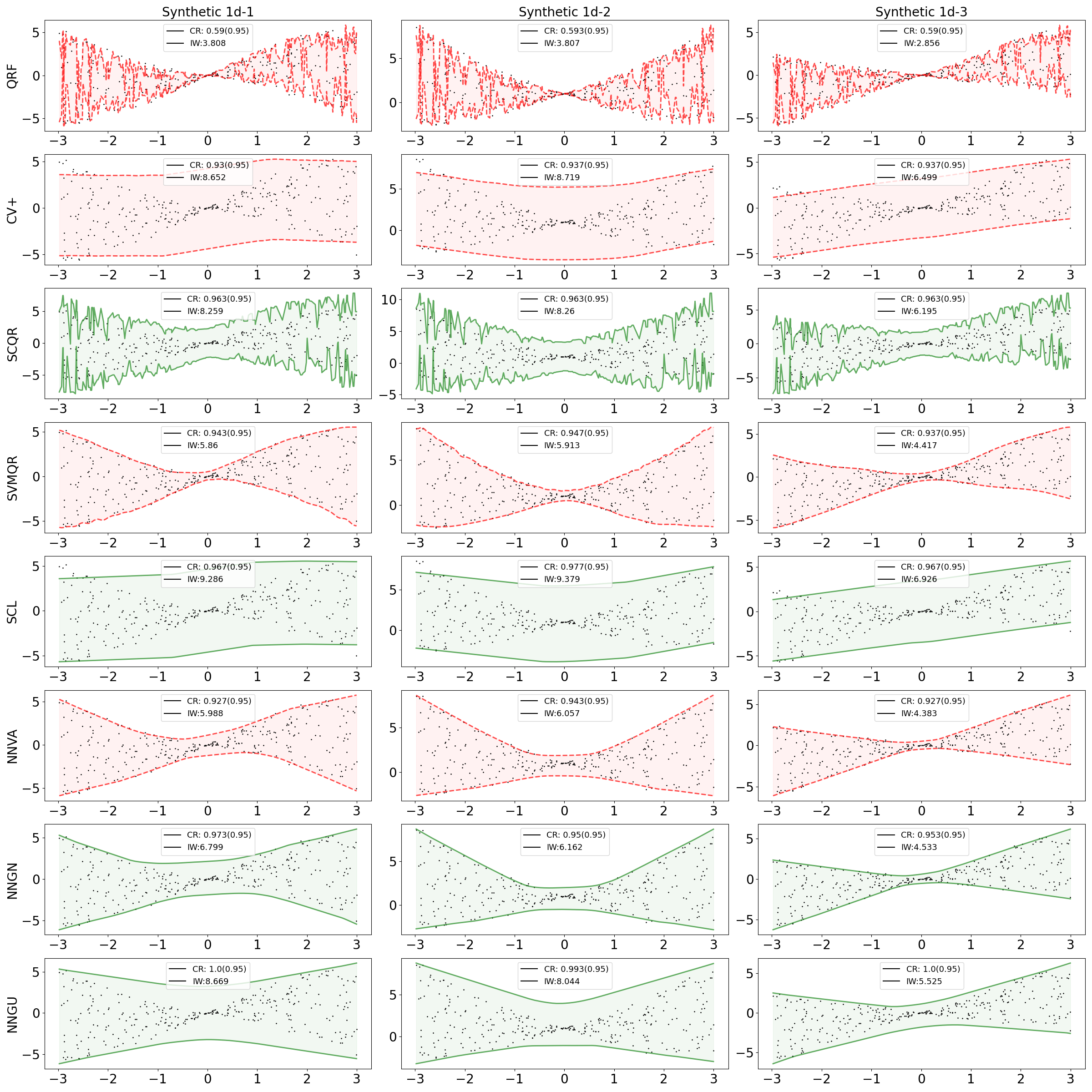
Refer to caption
Figure 1: Comparison of single PI constructions. PIs that attain 95%95\% target level are shown in solid and green lines, otherwise in dashed and red lines.

I.2 Pareto Curves

We illustrate the Pareto curves for the simultaneous PIs results with 19 target prediction levels in Section 6, in terms of the coverage rate (C​RCR) (X-axis) and the interval width (I​WIW) (Y-axis), to offer a more intuitive comparison. The titles of all plots are named as the datasets in Section 6. The arrangement of the plots are the same as the ones in Section I.1. Specifically, each subplot contains two curves, one constructed with (input coverage, width) and another constructed with (achieved coverage, width). The curve representing the input coverage and width is shown in dashed line while the one representing the achieved coverage and width is shown in solid line along with a 90%90\% confidence interval as the shaded area. Each point in the line denotes the average obtained from N=50N=50 repetitions of trials.

Ideally, a method performs well if in its Pareto curves, 1) the dashed line is on the left of the solid line, and 2) at the same time there is no level intersection between the solid line and the shaded area, meaning that within the same input coverage level, there is a sufficiently high probability in achieving the coverage level. Other than that, a smaller average I​WIW at each input coverage level is better since it refers to a less conservative predictive ability. From Figures 2 and 3, we notice that CV+, NNGN, and NNGU have a lot more cases where there is no intersection between the dashed line and shaded area while SCL, QRF, SVMQR, SCQR and NNVA do not. Also the former three methods tend to generate much shorter PIs than the others. Specifically, there are 55 datasets where there is no intersection between the dashed line and the shaded area for CV+ and NNGN, and 44 for NNGU. However, NNGN and NNGU can achieve a much shorter M​I​WMIW (average of I​WIW over all input coverage levels) than the rest of the methods.

One might notice that the two Pareto curves are a bit farther away from each other for NNVA, NNGN, and NNGU when the input coverage is small. This issue can be solved by choosing the calibration parameter more appropriately by, for example, training a more continuous spectrum of candidate models.

Refer to caption
Figure 2: Comparison of simultaneous PIs constructions in synthetic datasets 1 to 3, and Boston dataset. Dashed lines are constructed with (input coverage, width), and solid lines are constructed with (achieved coverage, width). Each point in the line denotes the average obtained from N=50N=50 repetitions of trials. Shaded area is the 90%90\% confidence interval.
Refer to caption
Figure 3: Comparison of simultaneous PIs constructions in Concrete, Energy, Wine and Yacht dataset. Dashed lines are constructed with (input coverage, width), and solid lines are constructed with (achieved coverage, width). Each point in the line denotes the average obtained from N=50N=50 repetitions of trials. Shaded area is the 90%90\% confidence interval.

I.3 Implementation Details

We elaborate more details about our experimental implementations in Sections 6 and I.1.

Datasets. Three synthetic datasets and five real-world benchmark datasets have been shown in Section 6. The real-world datasets are the open-access datasets “Boston”, “Concrete”, “Energy”, “Wine” and “Yacht” that have been widely used in previous studies (Hernández-Lobato and Adams 2015; Gal and Ghahramani 2016; Lakshminarayanan et al. 2017) for regression tasks. Table 4 shows their details.

Dataset N d Open-access Link
Boston: Boston Housing 506 13 kaggle.com/c/boston-housing
Concrete: Concrete Strength 1030 8 kaggle.com/aakashphadtare/concrete-data
Energy: Energy Efficiency 768 8 kaggle.com/elikplim/eergy-efficiency-dataset
Wine: Red Wine Quality 1599 11 kaggle.com/uciml/red-wine-quality-cortez-et-al-2009
Yacht: Yacht Hydrodynamics 308 6 archive.ics.uci.edu/ml/datasets/yacht+hydrodynamics
Table 4: Full names and details of benchmarking regression datasets. NN is the number of samples in the dataset and dd is the dimension of the feature vector.

The data are split into training and testing sets as follows. For the methods where validation data are needed for calibration (NNVA, NNGN, NNGU), we use a proportion of training data as the validation data. In the single PI case, all of the real-world datasets have 80%/20% training/testing split. For NN methods, “Boston” has 24%24\% of data for validation; “Concrete” has 16%16\% of data for validation; “Energy” has 10%10\% of data for validation; “Wine” has 12%12\% of data for validation; “Yacht” has 15%15\% of data for validation. The three multivariate synthetic datasets in Section 6 have 1600/3000 training/testing split. For NN methods, 350 data points are used for validation. In the simultaneous PIs case, all the real-world datasets have 80%/20% training/testing split. For NN methods, “Boston” has 24%24\% of data for validation; “Concrete” has 16%16\% of data for validation; “Energy” has 24%24\% of data for validation; “Wine” has 24%24\% of data for validation; “Yacht” has 24%24\% of data for validation. The three multivariate synthetic datasets in Section 6 have 1600/3000 training/testing split. For NN methods, 350 data points are used for validation. In addition, for the experiments in Section I.1, the three univariate synthetic datasets have 1200/300 training/testing split. For NN methods, 6060 data points are used for validation.

Implementations. We provide details of our algorithms and baseline approaches in Section 6. They appear in the same order as in Tables 1 and 2.

(1) QRF: quantile regression forests, as proposed in Meinshausen 2006. Our code is based on RandomForestQuantileRegressor from the package scikit-garden in Python.

(2) CV+: CV+ prediction interval, as proposed in Section 3 in Barber et al. 2019. In addition, the base regression algorithm is a neural network using mean square loss.

(3) SCQR: split conformalized quantile regression, as proposed in Algorithm 1 in Romano et al. 2019. The base quantile regression algorithm is exactly the QRF in (1).

(4) SVMQR: quantile regression via support vector machine, the code of which is available in Steinwart and Thomann 2017.

(5) SCL: split conformal learning with correction. The original split conformal learning is described in Algorithm 2 in Lei et al. 2018. The base regression algorithm is a neural network using mean square loss. Moreover, we apply a “correction” method to stipulate the coverage constraint with high confidence, which has been proposed in Equation 7 in Proposition 2b in Vovk 2012 to enhance the split/inductive conformal learning. Specifically, we change the prediction level 1−α1-\alpha to 1−α′1-\alpha^{\prime} by letting

β≥b​i​nnv,α​(⌊α′​(nv+1)−1⌋),\beta\geq bin_{n_{v},\alpha}(\lfloor\alpha^{\prime}(n_{v}+1)-1\rfloor),

where 1−β1-\beta is the prefixed confidence level (90% throughout our experiments), nvn_{v} is the size of the calibration set and b​i​nnv,αbin_{n_{v},\alpha} is the cumulative binomial distribution function with nvn_{v} trials and probability of success α\alpha.

(6) NNVA: neural networks using the loss shown in Section 6 with a vanilla scheme. In the vanilla scheme, we build multiple PI models by choosing different parameters λ>0\lambda>0 in the loss, and then select PIs with the smallest interval width among those whose empirical coverage rates on the validation dataset is larger than the target prediction levels, i.e., without the Gaussian margin in Algorithm 1.

(7) Ours-NNGN: neural networks using the loss shown in Section 6 with the normalized Gaussian PI calibration in Algorithm 1. We build multiple PI models by choosing different parameters λ>0\lambda>0 in the loss.

(8) Ours-NNGU: neural networks using the loss shown in Section 6 with the unnormalized Gaussian PI calibration in Algorithm 2. We build multiple PI models by choosing different parameters λ>0\lambda>0 in the loss.

For (6)(7)(8), in order to improve the training of the neural networks, we use the ensemble technique in Pearce et al. 2018. That is, instead of directly taking the outputs of one network, we train networks several times by using different initializations and then define the final prediction UU and LL as

U=U¯+1.96​σU, where ​U¯=1e​∑j=1eU^j,σU=1e−1​∑j=1e(U^j−U¯)2\displaystyle U=\overline{U}+1.96\sigma_{U},\text{ where }\overline{U}=\frac{1}{e}\sum_{j=1}^{e}\hat{U}_{j},\ \sigma_{U}=\frac{1}{e-1}\sum_{j=1}^{e}(\hat{U}_{j}-\overline{U})^{2}
L=L¯−1.96​σL, where ​L¯=1e​∑j=1eL^j,σL=1e−1​∑j=1e(L^j−L¯)2\displaystyle{L}=\overline{L}-1.96\sigma_{L},\text{ where }\overline{L}=\frac{1}{e}\sum_{j=1}^{e}\hat{L}_{j},\ \sigma_{L}=\frac{1}{e-1}\sum_{j=1}^{e}(\hat{L}_{j}-\overline{L})^{2}

where ee denotes the ensemble size.

Architectures and Hyper-parameters. For (2)(5)(6)(7)(8), we train fully connected neural networks with ReLU activations, using the Adam method for stochastic optimization. Note that the base neural networks in (2)(5) have only one output unit (point prediction) while our neural networks in (6)(7)(8) have two output units (lower and upper bounds of PIs). Nevertheless, the neural networks in (2)(5)(6)(7)(8) have the same architecture of hidden layers on each dataset. On “Boston” and “Concrete”, we have 1 hidden layer and each hidden layer has 5050 neurons. On “Energy”, “Wine” and “Yacht”, we have 2 hidden layers and each hidden layer has 6464 neurons. On three multivariate synthetic datasets in Section 6, we have 2 hidden layers and each hidden layer has 5050 neurons. On the three univariate synthetic datasets in Section I.1, we have 1 hidden layer and each hidden layer has 5050 neurons. In addition, N=50N=50 repetitions of trials are run on each dataset. The confidence level is 1−β=90%1-\beta=90\% in all experiments.

Appendix J Technical Proofs

J.1 Proofs for Results in Section 4

Proof of Theorem 4.1.

We first present a lemma:

Lemma J.1.

Let ξ\xi be a [0,1][0,1]-valued random variable such that 𝔼⁡[ξ]≤1−β\mathbb{E}[\xi]\leq 1-\beta for some β∈[0,1]\beta\in[0,1], then we have ℙ⁡(ξ≤1−β′)≥β−β′\mathbb{P}(\xi\leq 1-\beta^{\prime})\geq\beta-\beta^{\prime} for every β′∈(0,β)\beta^{\prime}\in(0,\beta).

Proof.

Define

ξ′:={0if ​ξ≤1−β′1−β′otherwise.\xi^{\prime}:=\begin{cases}0&\text{if }\xi\leq 1-\beta^{\prime}\\ 1-\beta^{\prime}&\text{otherwise}\end{cases}.

Then ξ≥ξ′\xi\geq\xi^{\prime} almost surely, hence

1−β≥𝔼⁡[ξ]≥𝔼⁡[ξ′]=(1−β′)​(1−ℙ⁡(ξ≤1−β′))1-\beta\geq\mathbb{E}[\xi]\geq\mathbb{E}[\xi^{\prime}]=(1-\beta^{\prime})(1-\mathbb{P}(\xi\leq 1-\beta^{\prime}))

which gives

ℙ⁡(ξ≤1−β′)≥β−β′1−β′≥β−β′.\mathbb{P}(\xi\leq 1-\beta^{\prime})\geq\frac{\beta-\beta^{\prime}}{1-\beta^{\prime}}\geq\beta-\beta^{\prime}.

∎

Now we turn to the main proof. For any ϵ>0\epsilon>0, let (Lϵ,Uϵ)∈ℋ×ℋ(L_{\epsilon},U_{\epsilon})\in\mathcal{H}\times\mathcal{H} be an ϵ\epsilon-optimal solution of (3.1), i.e., ℙπ​(Y∈[Lϵ​(X),Uϵ​(X)])≥1−α\mathbb{P}_{\pi}(Y\in[L_{\epsilon}(X),U_{\epsilon}(X)])\geq 1-\alpha and 𝔼πX​[Uϵ​(X)−Lϵ​(X)]≤R∗​(ℋ)+ϵ\mathbb{E}_{\pi_{X}}[U_{\epsilon}(X)-L_{\epsilon}(X)]\leq R^{*}(\mathcal{H})+\epsilon. Consider the enlarged interval Lϵc:=Lϵ−cL^{c}_{\epsilon}:=L_{\epsilon}-c, Uϵc:=Uϵ+cU^{c}_{\epsilon}:=U_{\epsilon}+c, where c≥0c\geq 0 is a constant. Let

P⁡(c):=ℙπ​(Y∈[Lϵc​(X),Uϵc​(X)])P(c):=\mathbb{P}_{\pi}(Y\in[L^{c}_{\epsilon}(X),U^{c}_{\epsilon}(X)])

be the coverage rate of the new interval. P⁡(c)P(c) satisfies limc→+∞P⁡(c)=1\lim_{c\to+\infty}P(c)=1 because of the continuity of measure, hence the smallest cc such that the coverage rate is above 1−α+t1-\alpha+t is finite, i.e.,

c∗:=inf{c≥0:P⁡(c)≥1−α+t}<∞.c^{*}:=\inf\big\{c\geq 0:P(c)\geq 1-\alpha+t\big\}<\infty.

We want to derive an upper bound for c∗c^{*}. If c∗=0c^{*}=0, every non-negative number is a valid upper bound, therefore we focus on the non-trivial case c∗>0c^{*}>0. In this case, we must have P⁡(c∗)=1−α+tP(c^{*})=1-\alpha+t due to continuity of the coverage probability function P⁡(⋅)P(\cdot). To explain the continuity of P⁡(⋅)P(\cdot), by conditioning on XX we can rewrite

P⁡(c)\displaystyle P(c) =\displaystyle= 𝔼πX​[ℙπ​(Y∈[Lϵc​(X),Uϵc​(X)]|X)]\displaystyle\mathbb{E}_{\pi_{X}}[\mathbb{P}_{\pi}(Y\in[L^{c}_{\epsilon}(X),U^{c}_{\epsilon}(X)]|X)] (J.1)
=\displaystyle= 𝔼πX​[∫Lϵ​(X)−cUϵ​(X)+cp⁡(y|X)​𝑑y]\displaystyle\mathbb{E}_{\pi_{X}}\Big[\int_{L_{\epsilon}(X)-c}^{U_{\epsilon}(X)+c}p(y|X)dy\Big]

and note that ∫Lϵ​(X)−cUϵ​(X)+cp⁡(y|X)​𝑑y\int_{L_{\epsilon}(X)-c}^{U_{\epsilon}(X)+c}p(y|X)dy is continuous in cc and bounded by 11 almost surely, therefore the continuity follows from bounded convergence theorem. For every c∈[0,c∗]c\in[0,c^{*}], we have P⁡(c)≤1−α+tP(c)\leq 1-\alpha+t by the definition of c∗c^{*}, hence applying Lemma J.1 to the conditioned form (J.1) of P⁡(c)P(c) gives

ℙπX​(ℙπ​(Y∈[Lϵc​(X),Uϵc​(X)]|X)≤1−α−t3)≥23​(α−t).\mathbb{P}_{\pi_{X}}\Big(\mathbb{P}_{\pi}(Y\in[L^{c}_{\epsilon}(X),U^{c}_{\epsilon}(X)]|X)\leq 1-\frac{\alpha-t}{3}\Big)\geq\frac{2}{3}(\alpha-t).

Now we write

1−α+t\displaystyle 1-\alpha+t =\displaystyle= P⁡(c∗)\displaystyle P(c^{*})
=\displaystyle= ℙπ​(Y∈[Lϵc∗​(X),Lϵ​(X))∪(Uϵ​(X),Uϵc∗​(X)])+ℙπ​(Y∈[Lϵ​(X),Uϵ​(X)])\displaystyle\mathbb{P}_{\pi}(Y\in[L_{\epsilon}^{c^{*}}(X),L_{\epsilon}(X))\cup(U_{\epsilon}(X),U_{\epsilon}^{c^{*}}(X)])+\mathbb{P}_{\pi}(Y\in[L_{\epsilon}(X),U_{\epsilon}(X)])
≥\displaystyle\geq 𝔼πX​[ℙπ​(Y∈[Lϵc∗​(X),Lϵ​(X))∪(Uϵ​(X),Uϵc∗​(X)]|X)]+1−α\displaystyle\mathbb{E}_{\pi_{X}}[\mathbb{P}_{\pi}(Y\in[L_{\epsilon}^{c^{*}}(X),L_{\epsilon}(X))\cup(U_{\epsilon}(X),U_{\epsilon}^{c^{*}}(X)]|X)]+1-\alpha
by conditioning on the XX and feasibility of (Lϵ,Uϵ)(L_{\epsilon},U_{\epsilon})
=\displaystyle= 𝔼πX​[∫0c∗p⁡(Lϵc​(X)|X)+p⁡(Uϵc​(X)|X)​𝑑c]+1−α\displaystyle\mathbb{E}_{\pi_{X}}\Big[\int_{0}^{c^{*}}p(L_{\epsilon}^{c}(X)|X)+p(U_{\epsilon}^{c}(X)|X)dc\Big]+1-\alpha
≥\displaystyle\geq 𝔼πX​[∫0c∗Γ⁡(X,1−ℙπ​(Y∈[Lϵc​(X),Uϵc​(X)]|X))​𝑑c]+1−α\displaystyle\mathbb{E}_{\pi_{X}}\Big[\int_{0}^{c^{*}}\Gamma\big(X,1-\mathbb{P}_{\pi}(Y\in[L_{\epsilon}^{c}(X),U_{\epsilon}^{c}(X)]|X)\big)dc\Big]+1-\alpha
by the definition of Γ⁡(⋅,⋅)\Gamma(\cdot,\cdot)
=\displaystyle= ∫0c∗𝔼πX​[Γ⁡(X,1−ℙπ​(Y∈[Lϵc​(X),Uϵc​(X)]|X))]​𝑑c+1−α\displaystyle\int_{0}^{c^{*}}\mathbb{E}_{\pi_{X}}\big[\Gamma\big(X,1-\mathbb{P}_{\pi}(Y\in[L_{\epsilon}^{c}(X),U_{\epsilon}^{c}(X)]|X)\big)\big]dc+1-\alpha
≥\displaystyle\geq ∫0c∗γα−t3​ℙπX​(ℙπ​(Y∈[Lϵc​(X),Uϵc​(X)]|X)≤1−α−t3​ and ​Γ​(X,α−t3)≥γα−t3)​𝑑c+1−α\displaystyle\int_{0}^{c^{*}}\gamma_{\frac{\alpha-t}{3}}\mathbb{P}_{\pi_{X}}\big(\mathbb{P}_{\pi}(Y\in[L_{\epsilon}^{c}(X),U_{\epsilon}^{c}(X)]|X)\leq 1-\frac{\alpha-t}{3}\text{ and }\Gamma(X,\frac{\alpha-t}{3})\geq\gamma_{\frac{\alpha-t}{3}}\big)dc+1-\alpha
≥\displaystyle\geq α−t3​γα−t3​c∗+1−α.\displaystyle\frac{\alpha-t}{3}\gamma_{\frac{\alpha-t}{3}}c^{*}+1-\alpha.

Therefore

c∗≤3​t(α−t)​γα−t3.c^{*}\leq\frac{3t}{(\alpha-t)\gamma_{\frac{\alpha-t}{3}}}.

Note that (Lϵc∗,Uϵc∗)(L_{\epsilon}^{c^{*}},U_{\epsilon}^{c^{*}}) is feasible for (4.1), therefore by optimality we have

Rt∗​(ℋ)\displaystyle R^{*}_{t}(\mathcal{H}) ≤\displaystyle\leq 𝔼πX​[Uϵc∗​(X)−Lϵc∗​(X)]\displaystyle\mathbb{E}_{\pi_{X}}[U_{\epsilon}^{c^{*}}(X)-L_{\epsilon}^{c^{*}}(X)]
≤\displaystyle\leq R∗​(ℋ)+ϵ+2​c∗\displaystyle R^{*}(\mathcal{H})+\epsilon+2c^{*}
≤\displaystyle\leq R∗​(ℋ)+ϵ+6​t(α−t)​γα−t3.\displaystyle R^{*}(\mathcal{H})+\epsilon+\frac{6t}{(\alpha-t)\gamma_{\frac{\alpha-t}{3}}}.

Since ϵ\epsilon is arbitrary, sending ϵ\epsilon to 00 completes the proof. ∎

Proof of Theorem 4.2.

Let ℋ^t2\hat{\mathcal{H}}^{2}_{t} and ℋt2\mathcal{H}^{2}_{t} be the feasible set of (3.2) and (4.1) respectively. When the events

Wϵ:={suph∈ℋ|𝔼π^X[h(X)]−𝔼πX[h(X)]|≤ϵ}W_{\epsilon}:=\big\{\sup_{h\in\mathcal{H}}\lvert\mathbb{E}_{\hat{\pi}_{X}}[h(X)]-\mathbb{E}_{\pi_{X}}[h(X)]\rvert\leq\epsilon\big\}

and

Ct:={supL,U∈ℋ​and​L≤U|ℙπ^X(Y∈[L(X),U(X)])−ℙπX(Y∈[L(X),U(X)])|≤t}C_{t}:=\big\{\sup_{L,U\in\mathcal{H}\;\text{and}\;L\leq U}\lvert\mathbb{P}_{\hat{\pi}_{X}}(Y\in[L(X),U(X)])-\mathbb{P}_{\pi_{X}}(Y\in[L(X),U(X)])\rvert\leq t\big\}

occur, it holds that ℋ2​t2⊂ℋ^t2⊂ℋ02\mathcal{H}^{2}_{2t}\subset\hat{\mathcal{H}}^{2}_{t}\subset\mathcal{H}^{2}_{0}, therefore (L^t∗,U^t∗)∈ℋ^t2⊂ℋ02(\hat{L}_{t}^{*},\hat{U}_{t}^{*})\in\hat{\mathcal{H}}^{2}_{t}\subset\mathcal{H}^{2}_{0} is feasible for (3.1). We also have

𝔼πX​[U^t∗​(X)−L^t∗​(X)]\displaystyle\mathbb{E}_{\pi_{X}}[\hat{U}_{t}^{*}(X)-\hat{L}_{t}^{*}(X)]
≤\displaystyle\leq 𝔼π^X​[U^t∗​(X)−L^t∗​(X)]+2​ϵ​ because of Wϵ\displaystyle\mathbb{E}_{\hat{\pi}_{X}}[\hat{U}_{t}^{*}(X)-\hat{L}_{t}^{*}(X)]+2\epsilon\text{\ \ because of $W_{\epsilon}$}
≤\displaystyle\leq inf(L,U)∈ℋ2​t2⊂ℋ^t2𝔼π^X​[U⁡(X)−L⁡(X)]+2​ϵ​ by optimality of (L^t∗,U^t∗) in ℋ^t2\displaystyle\inf_{(L,U)\in\mathcal{H}^{2}_{2t}\subset\hat{\mathcal{H}}^{2}_{t}}\mathbb{E}_{\hat{\pi}_{X}}[U(X)-L(X)]+2\epsilon\text{\ \ by optimality of $(\hat{L}_{t}^{*},\hat{U}_{t}^{*})$ in $\hat{\mathcal{H}}^{2}_{t}$}
≤\displaystyle\leq inf(L,U)∈ℋ2​t2𝔼πX​[U⁡(X)−L⁡(X)]+4​ϵ​ because of Wϵ\displaystyle\inf_{(L,U)\in\mathcal{H}^{2}_{2t}}\mathbb{E}_{\pi_{X}}[U(X)-L(X)]+4\epsilon\text{\ \ because of $W_{\epsilon}$}
=\displaystyle= ℛ2​t∗​(ℋ)+4​ϵ\displaystyle\mathcal{R}_{2t}^{*}(\mathcal{H})+4\epsilon
≤\displaystyle\leq ℛ∗​(ℋ)+12​t(α−2​t)​γα−2​t3+4​ϵ​ by Theorem 4.1.\displaystyle\mathcal{R}^{*}(\mathcal{H})+\frac{12t}{(\alpha-2t)\gamma_{\frac{\alpha-2t}{3}}}+4\epsilon\text{\ \ by Theorem \ref{sensitivity bound}}.

Note that ℙ⁡(Wϵ∩Ct)≥1−ℙ⁡(Wϵc)−ℙ⁡(Ctc)≥1−ϕ1​(n,ϵ,ℋ)−ϕ2​(n,t,ℋ)\mathbb{P}(W_{\epsilon}\cap C_{t})\geq 1-\mathbb{P}(W_{\epsilon}^{c})-\mathbb{P}(C_{t}^{c})\geq 1-\phi_{1}(n,\epsilon,\mathcal{H})-\phi_{2}(n,t,\mathcal{H}), concluding the theorem. ∎

Proof of Theorem 4.3.

We will need the following results:

Lemma J.2 (Adapted from Theorem 2.6.7 in Van der Vaart and Wellner 1996).

Let ‖g‖Q,2\|g\|_{Q,2} be the L2L_{2}-norm of a function gg under a probability measure QQ. For a VC-subgraph class 𝒢\mathcal{G} of functions from 𝒳\mathcal{X} to ℝ\mathbb{R}, and every probability measure QQ on 𝒳\mathcal{X}, we have for every ϵ∈(0,1)\epsilon\in(0,1)

N⁡(ϵ​‖G‖Q,2,𝒢,L2​(Q))≤C⁡(vc⁡(𝒢)+1)​(16​e)vc⁡(𝒢)+1​(1ϵ)2​v​c​(𝒢)N(\epsilon\|G\|_{Q,2},\mathcal{G},L_{2}(Q))\leq C(\mathrm{vc}\left(\mathcal{G}\right)+1)(16e)^{\mathrm{vc}\left(\mathcal{G}\right)+1}\big(\frac{1}{\epsilon}\big)^{2\mathrm{vc}\left(\mathcal{G}\right)}

where G⁡(x):=supg∈𝒢|g⁡(x)|G(x):=\sup_{g\in\mathcal{G}}\lvert g(x)\rvert is the envelope function of 𝒢\mathcal{G} and CC is a universal constant.

Lemma J.3 (Adapted from Theorem 2.14.1 in Van der Vaart and Wellner 1996).

Using the notations from Lemma J.2, we define

J⁡(𝒢):=supQ∫011+log⁡N⁡(ϵ​‖G‖Q,2,𝒢,L2​(Q))​𝑑ϵJ(\mathcal{G}):=\sup_{Q}\int_{0}^{1}\sqrt{1+\log N(\epsilon\|G\|_{Q,2},\mathcal{G},L_{2}(Q))}d\epsilon

where the supremum is taken over all discrete probability measures QQ with ‖G‖Q,2<∞\|G\|_{Q,2}<\infty. Then we have

‖supg∈𝒢|𝔼π^X​[g⁡(X)]−𝔼πX​[g⁡(X)]|‖1≤1n⋅C​J​(𝒢)​‖G‖2\|\sup_{g\in\mathcal{G}}\lvert\mathbb{E}_{\hat{\pi}_{X}}[g(X)]-\mathbb{E}_{\pi_{X}}[g(X)]\rvert\|_{1}\leq\frac{1}{\sqrt{n}}\cdot CJ(\mathcal{G})\|G\|_{2}

where the L1L_{1} norm ∥⋅∥1\|\cdot\|_{1} on the left hand size is with respect to the product measure πXn\pi_{X}^{n} (i.e., the data), and CC is a universal constant.

As a side note, a rigorous statement for the results in Lemma J.3 involves a so-called P-measurability condition for the class 𝒢\mathcal{G}, but we choose not to deal with the measurability requirement here. P-measurability holds for common function classes, e.g., if there exists a countable subclass 𝒢′⊂𝒢\mathcal{G}^{\prime}\subset\mathcal{G} such that for every g∈𝒢g\in\mathcal{G} there exists a sequence from 𝒢′\mathcal{G}^{\prime} that converges to gg point-wise. We need one more result:

Lemma J.4 (Adapted from Theorem 2.14.5 in Van der Vaart and Wellner 1996).

Using the notations from Lemma J.2, we have

‖supg∈𝒢|𝔼π^X​[g⁡(X)]−𝔼πX​[g⁡(X)]|‖ψ2\displaystyle\|\sup_{g\in\mathcal{G}}\lvert\mathbb{E}_{\hat{\pi}_{X}}[g(X)]-\mathbb{E}_{\pi_{X}}[g(X)]\rvert\|_{\psi_{2}}
≤\displaystyle\leq C⁡(‖supg∈𝒢|𝔼π^X​[g⁡(X)]−𝔼πX​[g⁡(X)]|‖1+1n⋅‖G‖ψ2)\displaystyle C\big(\|\sup_{g\in\mathcal{G}}\lvert\mathbb{E}_{\hat{\pi}_{X}}[g(X)]-\mathbb{E}_{\pi_{X}}[g(X)]\rvert\|_{1}+\frac{1}{\sqrt{n}}\cdot\|G\|_{\psi_{2}}\big)

where the sub-Gaussian norm ∥⋅∥ψ2\|\cdot\|_{\psi_{2}} on the left hand size is with respect to the product measure πXn\pi_{X}^{n} (i.e., the data), and CC is a universal constant.

We now turn to the main proof. We first deal with ϕ1\phi_{1}. Consider the centered class ℋc:={h−𝔼πX​[h⁡(X)]:h∈ℋ}\mathcal{H}_{c}:=\{h-\mathbb{E}_{\pi_{X}}[h(X)]:h\in\mathcal{H}\}, whose envelope function is HH. Since ℋc⊂ℋ+\mathcal{H}_{c}\subset\mathcal{H}_{+}, we have vc⁡(ℋc)≤vc⁡(ℋ+)\mathrm{vc}\left(\mathcal{H}_{c}\right)\leq\mathrm{vc}\left(\mathcal{H}_{+}\right). We calculate the complexity measure J⁡(ℋc)J(\mathcal{H}_{c}) from Lemma J.3

J⁡(ℋc)\displaystyle J(\mathcal{H}_{c}) =\displaystyle= supQ∫011+log⁡N⁡(ϵ​‖H‖Q,2,ℋc,L2​(Q))​𝑑ϵ\displaystyle\sup_{Q}\int_{0}^{1}\sqrt{1+\log N(\epsilon\|H\|_{Q,2},\mathcal{H}_{c},L_{2}(Q))}d\epsilon
≤\displaystyle\leq ∫01(1+2​(vc⁡(ℋc)+1)​log⁡1ϵ+16​(vc⁡(ℋc)+1)+log⁡(vc⁡(ℋc)+1)+log⁡C)12​𝑑ϵ\displaystyle\int_{0}^{1}\Big(1+2(\mathrm{vc}\left(\mathcal{H}_{c}\right)+1)\log\frac{1}{\epsilon}+16(\mathrm{vc}\left(\mathcal{H}_{c}\right)+1)+\log(\mathrm{vc}\left(\mathcal{H}_{c}\right)+1)+\log C\Big)^{\frac{1}{2}}d\epsilon
  by Lemma J.2
≤\displaystyle\leq 1+16​(vc⁡(ℋc)+1)+log⁡(vc⁡(ℋc)+1)+log⁡C+∫012​(vc⁡(ℋc)+1)​log⁡1ϵ​𝑑ϵ\displaystyle\sqrt{1+16(\mathrm{vc}\left(\mathcal{H}_{c}\right)+1)+\log(\mathrm{vc}\left(\mathcal{H}_{c}\right)+1)+\log C}+\int_{0}^{1}\sqrt{2(\mathrm{vc}\left(\mathcal{H}_{c}\right)+1)\log\frac{1}{\epsilon}}d\epsilon
≤\displaystyle\leq C​vc⁡(ℋc)​ for another universal constant ​C\displaystyle C\sqrt{\mathrm{vc}\left(\mathcal{H}_{c}\right)}\text{\ \ \ for another universal constant }C
≤\displaystyle\leq C​vc⁡(ℋ+).\displaystyle C\sqrt{\mathrm{vc}\left(\mathcal{H}_{+}\right)}.

Applying the bound in Lemma J.3 to the class ℋc\mathcal{H}_{c} gives

‖suph∈ℋc|𝔼π^X​[h⁡(X)]−𝔼πX​[h⁡(X)]|‖1≤vc⁡(ℋ+)n⋅C​‖H‖2.\|\sup_{h\in\mathcal{H}_{c}}\lvert\mathbb{E}_{\hat{\pi}_{X}}[h(X)]-\mathbb{E}_{\pi_{X}}[h(X)]\rvert\|_{1}\leq\sqrt{\frac{\mathrm{vc}\left(\mathcal{H}_{+}\right)}{n}}\cdot C\|H\|_{2}.

Further applying Lemma J.4, and using the fact that ∥⋅∥2≤C∥⋅∥ψ2\|\cdot\|_{2}\leq C\|\cdot\|_{\psi_{2}} for some universal constant CC lead to

‖suph∈ℋc|𝔼π^X​[h⁡(X)]−𝔼πX​[h⁡(X)]|‖ψ2≤vc⁡(ℋ+)n⋅C​‖H‖ψ2.\|\sup_{h\in\mathcal{H}_{c}}\lvert\mathbb{E}_{\hat{\pi}_{X}}[h(X)]-\mathbb{E}_{\pi_{X}}[h(X)]\rvert\|_{\psi_{2}}\leq\sqrt{\frac{\mathrm{vc}\left(\mathcal{H}_{+}\right)}{n}}\cdot C\|H\|_{\psi_{2}}.

Finally, note that suph∈ℋ|𝔼π^X​[h⁡(X)]−𝔼πX​[h⁡(X)]|=suph∈ℋc|𝔼π^X​[h⁡(X)]−𝔼πX​[h⁡(X)]|\sup_{h\in\mathcal{H}}\lvert\mathbb{E}_{\hat{\pi}_{X}}[h(X)]-\mathbb{E}_{\pi_{X}}[h(X)]\rvert=\sup_{h\in\mathcal{H}_{c}}\lvert\mathbb{E}_{\hat{\pi}_{X}}[h(X)]-\mathbb{E}_{\pi_{X}}[h(X)]\rvert, therefore the same bound holds for ‖suph∈ℋ|𝔼π^X​[h⁡(X)]−𝔼πX​[h⁡(X)]|‖ψ2\|\sup_{h\in\mathcal{H}}\lvert\mathbb{E}_{\hat{\pi}_{X}}[h(X)]-\mathbb{E}_{\pi_{X}}[h(X)]\rvert\|_{\psi_{2}}. The sub-Gaussian tail bound then gives the expression for ϕ1\phi_{1}.

Next we analyze ϕ2\phi_{2}. First note that ℋ⊂ℋ+\mathcal{H}\subset\mathcal{H}_{+}, therefore vc⁡(ℋ)≤vc⁡(ℋ+)\mathrm{vc}\left(\mathcal{H}\right)\leq\mathrm{vc}\left(\mathcal{H}_{+}\right). By the definition of VC-subgraph, both its closed subgraph class 𝒮u​p​p​e​r:={{(x,y):y≤U⁡(x)}:U∈ℋ}\mathcal{S}_{upper}:=\{\{(x,y):y\leq U(x)\}:U\in\mathcal{H}\} and open subgraph class 𝒮l​o​w​e​r′:={{(x,y):y<L⁡(x)}:L∈ℋ}\mathcal{S}^{\prime}_{lower}:=\{\{(x,y):y<L(x)\}:L\in\mathcal{H}\} have a VC dimension vc⁡(𝒮u​p​p​e​r)=vc⁡(𝒮l​o​w​e​r′)=vc⁡(ℋ)\mathrm{vc}\left(\mathcal{S}_{upper}\right)=\mathrm{vc}\left(\mathcal{S}^{\prime}_{lower}\right)=\mathrm{vc}\left(\mathcal{H}\right) (using ≤\leq or << for defining subgraphs does not affect the resulting VC dimension, see Problem 10 from Section 2.6 in Van der Vaart and Wellner 1996). To proceed, we need the following preservation result for VC classes:

Lemma J.5 (Adapted from Lemma 9.7 statements (i) and (v) in Kosorok 2007).

Let 𝒮\mathcal{S} be a VC class of sets in a space 𝕊\mathbb{S}, then

1.

ψ:𝕊→𝕊\psi:\mathbb{S}\to\mathbb{S} be a one-to-one mapping, then the class ψ⁡(𝒮):={{ψ⁡(s):s∈S}:S∈𝒮}\psi(\mathcal{S}):=\{\{\psi(s):s\in S\}:S\in\mathcal{S}\} is also a VC class with vc⁡(ψ⁡(𝒮))=vc⁡(𝒮)\mathrm{vc}\left(\psi(\mathcal{S})\right)=\mathrm{vc}\left(\mathcal{S}\right)

2.

The complement class 𝒮c:={𝕊\S:S∈𝒮}\mathcal{S}^{c}:=\{\mathbb{S}\backslash S:S\in\mathcal{S}\} is a VC class with vc⁡(𝒮c)=vc⁡(𝒮)\mathrm{vc}\left(\mathcal{S}^{c}\right)=\mathrm{vc}\left(\mathcal{S}\right).

and a VC dimension bound for unions and intersections of VC classes:

Lemma J.6 (Adapted from Theorem 1.1 in Van Der Vaart and Wellner 2009).

Suppose 𝒮1,…,𝒮K\mathcal{S}_{1},\ldots,\mathcal{S}_{K} are VC classes of sets in a space 𝕊\mathbb{S}. Define ⊔k=1K𝒮k:={∪k=1KSk:Sk∈𝒮k for k=1,…,K}\sqcup_{k=1}^{K}\mathcal{S}_{k}:=\{\cup_{k=1}^{K}S_{k}:S_{k}\in\mathcal{S}_{k}\text{ for }k=1,\ldots,K\} and ⊓k=1K𝒮k:={∩k=1KSk:Sk∈𝒮k for k=1,…,K}\sqcap_{k=1}^{K}\mathcal{S}_{k}:=\{\cap_{k=1}^{K}S_{k}:S_{k}\in\mathcal{S}_{k}\text{ for }k=1,\ldots,K\}. We have

vc(⊔k=1K𝒮k)≤Clog(K)∑k=1Kvc(𝒮k),vc(⊓k=1K𝒮k)≤Clog(K)∑k=1Kvc(𝒮k)\mathrm{vc}\left(\sqcup_{k=1}^{K}\mathcal{S}_{k}\right)\leq C\log(K)\sum_{k=1}^{K}\mathrm{vc}\left(\mathcal{S}_{k}\right),\;\;\;\mathrm{vc}\left(\sqcap_{k=1}^{K}\mathcal{S}_{k}\right)\leq C\log(K)\sum_{k=1}^{K}\mathrm{vc}\left(\mathcal{S}_{k}\right)

for some universal constant CC.

Further consider 𝒮l​o​w​e​r:={{(x,y):y≥L⁡(x)}:L∈ℋ}\mathcal{S}_{lower}:=\{\{(x,y):y\geq L(x)\}:L\in\mathcal{H}\}, and 𝒮b​t​w:={{(x,y):L(x)≤y≤U(x)}:L,U∈ℋ and L≤U}\mathcal{S}_{btw}:=\{\{(x,y):L(x)\leq y\leq U(x)\}:L,U\in\mathcal{H}\text{ and }L\leq U\}. We observe that 𝒮l​o​w​e​r=𝒮l​o​w​e​r′c\mathcal{S}_{lower}=\mathcal{S}_{lower}^{\prime c}, and that 𝒮b​t​w⊂𝒮l​o​w​e​r⊓𝒮u​p​p​e​r\mathcal{S}_{btw}\subset\mathcal{S}_{lower}\sqcap\mathcal{S}_{upper}. Therefore by Lemma J.5 we have vc⁡(𝒮l​o​w​e​r)=vc⁡(𝒮l​o​w​e​r′)\mathrm{vc}\left(\mathcal{S}_{lower}\right)=\mathrm{vc}\left(\mathcal{S}^{\prime}_{lower}\right), and applying the bound for intersection from Lemma J.6 to 𝒮b​t​w\mathcal{S}_{btw} gives vc⁡(𝒮b​t​w)≤vc⁡(𝒮l​o​w​e​r⊓𝒮u​p​p​e​r)≤C​vc​(𝒮u​p​p​e​r)=C​vc​(ℋ)\mathrm{vc}\left(\mathcal{S}_{btw}\right)\leq\mathrm{vc}\left(\mathcal{S}_{lower}\sqcap\mathcal{S}_{upper}\right)\leq C\mathrm{vc}\left(\mathcal{S}_{upper}\right)=C\mathrm{vc}\left(\mathcal{H}\right) for some universal constant CC. With this VC bound for 𝒮b​t​w\mathcal{S}_{btw}, we are ready to use standard deviation bounds for VC set classes (see, e.g., equation (3.3) in Vapnik 2013) to get

supL,U∈ℋ​and​L≤Uℙ⁡(|ℙπ^​(L⁡(X)≤Y≤U⁡(X))−ℙπ​(L⁡(X)≤Y≤U⁡(X))|>t)\displaystyle\sup_{L,U\in\mathcal{H}\;\text{and}\;L\leq U}\mathbb{P}(\lvert\mathbb{P}_{\hat{\pi}}(L(X)\leq Y\leq U(X))-\mathbb{P}_{\pi}(L(X)\leq Y\leq U(X))\rvert>t)
=\displaystyle= supS∈𝒮b​t​wℙ⁡(|ℙπ^​((X,Y)∈S)−ℙπ​((X,Y)∈S)|>t)\displaystyle\sup_{S\in\mathcal{S}_{btw}}\mathbb{P}(\lvert\mathbb{P}_{\hat{\pi}}((X,Y)\in S)-\mathbb{P}_{\pi}((X,Y)\in S)\rvert>t)
≤\displaystyle\leq 4​G​r​o​w​t​h​(2​n)​exp⁡(−t2​n)\displaystyle 4\mathrm{Growth}(2n)\exp(-t^{2}n)

where Growth⁡(2​n)\mathrm{Growth}(2n) is the growth function, or the shattering number, for the class 𝒮b​t​w\mathcal{S}_{btw}. By the Sauer–Shelah lemma we have Growth⁡(2​n)=22​n\mathrm{Growth}(2n)=2^{2n} if 2​n<vc⁡(𝒮b​t​w)2n<\mathrm{vc}\left(\mathcal{S}_{btw}\right) and ≤(2​e​nvc⁡(𝒮b​t​w))vc⁡(𝒮b​t​w)\leq\big(\frac{2en}{\mathrm{vc}\left(\mathcal{S}_{btw}\right)}\big)^{\mathrm{vc}\left(\mathcal{S}_{btw}\right)} if 2​n≥vc⁡(𝒮b​t​w)2n\geq\mathrm{vc}\left(\mathcal{S}_{btw}\right). With the upper bound for vc⁡(𝒮b​t​w)\mathrm{vc}\left(\mathcal{S}_{btw}\right), we can bound

Growth⁡(2​n)≤{22​nif ​2​n<C​vc​(ℋ)(2​e​nC​vc​(ℋ))C​vc​(ℋ)if ​2​n≥C​vc​(ℋ)\mathrm{Growth}(2n)\leq\begin{cases}2^{2n}&\text{if }2n<C\mathrm{vc}\left(\mathcal{H}\right)\\ \big(\frac{2en}{C\mathrm{vc}\left(\mathcal{H}\right)}\big)^{C\mathrm{vc}\left(\mathcal{H}\right)}&\text{if }2n\geq C\mathrm{vc}\left(\mathcal{H}\right)\end{cases}

giving rise to our formula for ϕ2\phi_{2}.

The feasibility and optimality bound for δ^t∗\hat{\delta}_{t}^{*} can be obtained by solving ϕ1​(n,ϵ,ℋ)=η2\phi_{1}(n,\epsilon,\mathcal{H})=\frac{\eta}{2} and ϕ2​(n,t,ℋ)=η2\phi_{2}(n,t,\mathcal{H})=\frac{\eta}{2} for ϵ\epsilon and tt, and then applying Theorem 4.2. ∎

Proof of Theorem 4.4.

We first treat ϕ1\phi_{1}. We need a maximal inequality that is similar to Lemma J.3, but based on bracketing numbers instead:

Lemma J.7 (Adapted from Theorem 2.14.2 in Van der Vaart and Wellner 1996).

Using the notations from Lemma J.2, for a function class 𝒢\mathcal{G} we define

J[]​(𝒢):=∫011+log⁡N⁡(ϵ​‖G‖πX,2,𝒢,L2​(πX))​𝑑ϵ.J_{[]}(\mathcal{G}):=\int_{0}^{1}\sqrt{1+\log N(\epsilon\|G\|_{\pi_{X},2},\mathcal{G},L_{2}(\pi_{X}))}d\epsilon.

Then we have

‖supg∈𝒢|𝔼π^X​[g⁡(X)]−𝔼πX​[g⁡(X)]|‖1≤1n⋅C​J[]​(𝒢)​‖G‖2\|\sup_{g\in\mathcal{G}}\lvert\mathbb{E}_{\hat{\pi}_{X}}[g(X)]-\mathbb{E}_{\pi_{X}}[g(X)]\rvert\|_{1}\leq\frac{1}{\sqrt{n}}\cdot CJ_{[]}(\mathcal{G})\|G\|_{2}

where the L1L_{1} norm ∥⋅∥1\|\cdot\|_{1} on the left hand size is with respect to the product measure πXn\pi_{X}^{n} (i.e., the data), and CC is a universal constant.

We consider the centered class ℋc:={h−𝔼πX​[h⁡(X)]:h∈ℋ}\mathcal{H}_{c}:=\{h-\mathbb{E}_{\pi_{X}}[h(X)]:h\in\mathcal{H}\} as in the proof of Theorem 4.3. Note that, by Jensen’s inequality, the Lipschitzness condition stipulates that |𝔼πX​[h⁡(X,θ1)]−𝔼πX​[h⁡(X,θ2)]|≤‖ℒ‖1​‖θ1−θ2‖2\lvert\mathbb{E}_{\pi_{X}}[h(X,\theta_{1})]-\mathbb{E}_{\pi_{X}}[h(X,\theta_{2})]\rvert\leq\|\mathcal{L}\|_{1}\|\theta_{1}-\theta_{2}\|_{2}, therefore the centered class is also Lipschitz in θ\theta, with a slightly larger coefficient

|h⁡(x,θ1)−𝔼πX​[h⁡(X,θ1)]−(h⁡(x,θ2)−𝔼πX​[h⁡(X,θ2)])|≤(ℒ⁡(x)+‖ℒ‖1)​‖θ1−θ2‖2.\lvert h(x,\theta_{1})-\mathbb{E}_{\pi_{X}}[h(X,\theta_{1})]-(h(x,\theta_{2})-\mathbb{E}_{\pi_{X}}[h(X,\theta_{2})])\rvert\leq(\mathcal{L}(x)+\|\mathcal{L}\|_{1})\|\theta_{1}-\theta_{2}\|_{2}.

The envelope function of ℋc\mathcal{H}_{c} is HH. We then calculate the bracketing number of ℋc\mathcal{H}_{c}. Using the Lipschitzness condition, the bracketing number of ℋc\mathcal{H}_{c} can be bounded by the covering number of the parameter space Θ\Theta as below

N[](4ϵ∥ℒ∥2,ℋc,L2(πX))≤N(ϵ,Θ,∥⋅∥2)N_{[]}(4\epsilon\|\mathcal{L}\|_{2},\mathcal{H}_{c},L_{2}(\pi_{X}))\leq N(\epsilon,\Theta,\|\cdot\|_{2})

where N(ϵ,Θ,∥⋅∥2)N(\epsilon,\Theta,\|\cdot\|_{2}) is the ϵ\epsilon-covering number of Θ\Theta with respect to the l2l_{2} norm, i.e., the minimum number of l2l_{2}-balls of size ϵ\epsilon needed to cover Θ\Theta. Since Θ\Theta is bounded, its covering number is upper bounded by that of the l2l_{2}-ball of radius diam⁡(Θ)\mathrm{diam}\left(\Theta\right), which is further bounded by (3​d​i​a​m​(Θ)ϵ)l\big(\frac{3\mathrm{diam}\left(\Theta\right)}{\epsilon}\big)^{l} (see Problem 6 from Section 2.1 in Van der Vaart and Wellner 1996). All these lead to

N[](ϵ∥H∥2,ℋc,L2(πX))≤N(ϵ​‖H‖24​‖ℒ‖2,Θ,∥⋅∥2)≤(12​d​i​a​m​(Θ)​‖ℒ‖2ϵ​‖H‖2)l.N_{[]}(\epsilon\|H\|_{2},\mathcal{H}_{c},L_{2}(\pi_{X}))\leq N(\frac{\epsilon\|H\|_{2}}{4\|\mathcal{L}\|_{2}},\Theta,\|\cdot\|_{2})\leq\big(\frac{12\mathrm{diam}\left(\Theta\right)\|\mathcal{L}\|_{2}}{\epsilon\|H\|_{2}}\big)^{l}.

Also note that when ϵ≥4​d​i​a​m​(Θ)​‖ℒ‖2‖H‖2\epsilon\geq\frac{4\mathrm{diam}\left(\Theta\right)\|\mathcal{L}\|_{2}}{\|H\|_{2}} the bracketing number N[]​(ϵ​‖H‖2,ℋc,L2​(πX))=1N_{[]}(\epsilon\|H\|_{2},\mathcal{H}_{c},L_{2}(\pi_{X}))=1 because N(diam(Θ),Θ,∥⋅∥2)=1N(\mathrm{diam}\left(\Theta\right),\Theta,\|\cdot\|_{2})=1. We can now compute the complexity measure J[]​(ℋc)J_{[]}(\mathcal{H}_{c}) as follows

J[]​(ℋc)\displaystyle J_{[]}(\mathcal{H}_{c}) ≤\displaystyle\leq ∫0min⁡{1,4​d​i​a​m​(Θ)​‖ℒ‖2‖H‖2}1+l​log⁡12​diam​(Θ)​‖ℒ‖2ϵ​‖H‖2​𝑑ϵ+1−min⁡{1,4​diam​(Θ)​‖ℒ‖2‖H‖2}\displaystyle\int_{0}^{\min\{1,\frac{4\mathrm{diam}\left(\Theta\right)\|\mathcal{L}\|_{2}}{\|H\|_{2}}\}}\sqrt{1+l\log\frac{12\mathrm{diam}\left(\Theta\right)\|\mathcal{L}\|_{2}}{\epsilon\|H\|_{2}}}d\epsilon+1-\min\{1,\frac{4\mathrm{diam}\left(\Theta\right)\|\mathcal{L}\|_{2}}{\|H\|_{2}}\}
≤\displaystyle\leq 1+l​∫0min⁡{1,4​d​i​a​m​(Θ)​‖ℒ‖2‖H‖2}log⁡12​diam​(Θ)​‖ℒ‖2ϵ​‖H‖2​𝑑ϵ\displaystyle 1+\sqrt{l}\int_{0}^{\min\{1,\frac{4\mathrm{diam}\left(\Theta\right)\|\mathcal{L}\|_{2}}{\|H\|_{2}}\}}\sqrt{\log\frac{12\mathrm{diam}\left(\Theta\right)\|\mathcal{L}\|_{2}}{\epsilon\|H\|_{2}}}d\epsilon
=\displaystyle= 1+l⋅12​diam​(Θ)​‖ℒ‖2‖H‖2∫0min⁡{13,‖H‖212​d​i​a​m​(Θ)​‖ℒ‖2}log⁡1ϵdϵ\displaystyle 1+\sqrt{l}\cdot\frac{12\mathrm{diam}\left(\Theta\right)\|\mathcal{L}\|_{2}}{\|H\|_{2}}\int_{0}^{\min\{\frac{1}{3},\frac{\|H\|_{2}}{12\mathrm{diam}\left(\Theta\right)\|\mathcal{L}\|_{2}}\}}\sqrt{\log\frac{1}{\epsilon}}d\epsilon
=\displaystyle= 1+C​l⋅12​diam​(Θ)​‖ℒ‖2‖H‖2​log⁡max​{3,12​diam​(Θ)​‖ℒ‖2‖H‖2}⋅min⁡{13,‖H‖212​diam​(Θ)​‖ℒ‖2}\displaystyle 1+C\sqrt{l}\cdot\frac{12\mathrm{diam}\left(\Theta\right)\|\mathcal{L}\|_{2}}{\|H\|_{2}}\sqrt{\log\max\{3,\frac{12\mathrm{diam}\left(\Theta\right)\|\mathcal{L}\|_{2}}{\|H\|_{2}}\}}\cdot\min\{\frac{1}{3},\frac{\|H\|_{2}}{12\mathrm{diam}\left(\Theta\right)\|\mathcal{L}\|_{2}}\}
  by Lemma J.8 below
≤\displaystyle\leq 1+C​l⋅log⁡max​{3,12​diam​(Θ)​‖ℒ‖2‖H‖2}⋅min⁡{4​diam​(Θ)​‖ℒ‖2‖H‖2,1}\displaystyle 1+C\sqrt{l}\cdot\sqrt{\log\max\{3,\frac{12\mathrm{diam}\left(\Theta\right)\|\mathcal{L}\|_{2}}{\|H\|_{2}}\}}\cdot\min\{\frac{4\mathrm{diam}\left(\Theta\right)\|\mathcal{L}\|_{2}}{\|H\|_{2}},1\}
≤\displaystyle\leq C​l⋅max⁡{log⁡diam⁡(Θ)​‖ℒ‖2‖H‖2,1}.\displaystyle C\sqrt{l}\cdot\sqrt{\max\{\log\frac{\mathrm{diam}\left(\Theta\right)\|\mathcal{L}\|_{2}}{\|H\|_{2}},1\}}.
Lemma J.8.

For every c∈(0,13]c\in(0,\frac{1}{3}], we have

∫0clog⁡1ϵ​𝑑ϵ≤C⋅c​log⁡1c\int_{0}^{c}\sqrt{\log\frac{1}{\epsilon}}d\epsilon\leq C\cdot c\sqrt{\log\frac{1}{c}}

where CC is a universal constant.

Proof of Lemma J.8.

By a change of variable t=log⁡1ϵt=\sqrt{\log\frac{1}{\epsilon}}, we write

∫0clog⁡1ϵ​𝑑ϵ\displaystyle\int_{0}^{c}\sqrt{\log\frac{1}{\epsilon}}d\epsilon =\displaystyle= ∫log⁡1c∞2​t2​exp⁡(−t2)​𝑑t\displaystyle\int_{\sqrt{\log\frac{1}{c}}}^{\infty}2t^{2}\exp(-t^{2})dt
=\displaystyle= −t​exp⁡(−t2)|t=log⁡1ct=∞+∫log⁡1c∞exp⁡(−t2)​𝑑t\displaystyle-t\exp(-t^{2})\Big|_{t=\sqrt{\log\frac{1}{c}}}^{t=\infty}+\int_{\sqrt{\log\frac{1}{c}}}^{\infty}\exp(-t^{2})dt
≤\displaystyle\leq c​log⁡1c+∫log⁡1c∞tlog⁡1c​exp⁡(−t2)​𝑑t\displaystyle c\sqrt{\log\frac{1}{c}}+\int_{\sqrt{\log\frac{1}{c}}}^{\infty}\frac{t}{\sqrt{\log\frac{1}{c}}}\exp(-t^{2})dt
=\displaystyle= c​log⁡1c+c2​log⁡1c≤(1+12​log⁡3)​c​log⁡1c\displaystyle c\sqrt{\log\frac{1}{c}}+\frac{c}{2\sqrt{\log\frac{1}{c}}}\leq\big(1+\frac{1}{2\log 3}\big)c\sqrt{\log\frac{1}{c}}

where in the last line we use c≤13c\leq\frac{1}{3}. ∎

Lemma J.7 then entails the following maximal inequality for the centered class ℋc\mathcal{H}_{c}

‖suph∈ℋc|𝔼π^X​[h⁡(X)]−𝔼πX​[h⁡(X)]|‖1≤ln⋅C​max⁡{log⁡diam⁡(Θ)​‖ℒ‖2‖H‖2,1}​‖H‖2.\|\sup_{h\in\mathcal{H}_{c}}\lvert\mathbb{E}_{\hat{\pi}_{X}}[h(X)]-\mathbb{E}_{\pi_{X}}[h(X)]\rvert\|_{1}\leq\sqrt{\frac{l}{n}}\cdot C\sqrt{\max\{\log\frac{\mathrm{diam}\left(\Theta\right)\|\mathcal{L}\|_{2}}{\|H\|_{2}},1\}}\|H\|_{2}.

Further applying Lemma J.4 gives

‖suph∈ℋc|𝔼π^X​[h⁡(X)]−𝔼πX​[h⁡(X)]|‖ψ2≤ln⋅C​max⁡{log⁡diam⁡(Θ)​‖ℒ‖2‖H‖2,1}​‖H‖ψ2.\|\sup_{h\in\mathcal{H}_{c}}\lvert\mathbb{E}_{\hat{\pi}_{X}}[h(X)]-\mathbb{E}_{\pi_{X}}[h(X)]\rvert\|_{\psi_{2}}\leq\sqrt{\frac{l}{n}}\cdot C\sqrt{\max\{\log\frac{\mathrm{diam}\left(\Theta\right)\|\mathcal{L}\|_{2}}{\|H\|_{2}},1\}}\|H\|_{\psi_{2}}.

Finally, note that suph∈ℋ|𝔼π^X​[h⁡(X)]−𝔼πX​[h⁡(X)]|=suph∈ℋc|𝔼π^X​[h⁡(X)]−𝔼πX​[h⁡(X)]|\sup_{h\in\mathcal{H}}\lvert\mathbb{E}_{\hat{\pi}_{X}}[h(X)]-\mathbb{E}_{\pi_{X}}[h(X)]\rvert=\sup_{h\in\mathcal{H}_{c}}\lvert\mathbb{E}_{\hat{\pi}_{X}}[h(X)]-\mathbb{E}_{\pi_{X}}[h(X)]\rvert, hence the same sub-Gaussian norm holds for the original class ℋ\mathcal{H} too. The tail bound ϕ1\phi_{1} follows from the sub-Gaussian tail bound.

Secondly, we analyze ϕ2\phi_{2}. We first calculate the bracketing number of the corresponding indicator class

ℋi​n​d:={(x,y)→Ih⁡(x,θl)≤y≤h⁡(x,θu):θl,θu∈Θ, and h(⋅,θl)≤h(⋅,θu)}.\mathcal{H}_{ind}:=\{(x,y)\to I_{h(x,\theta_{l})\leq y\leq h(x,\theta_{u})}:\theta_{l},\theta_{u}\in\Theta,\text{ and }h(\cdot,\theta_{l})\leq h(\cdot,\theta_{u})\}.

For fixed θlo,θuo∈Θ\theta_{l}^{o},\theta_{u}^{o}\in\Theta and ϵ>0\epsilon>0, consider a bracket enclosed by

lo​(x,y)\displaystyle l^{o}(x,y) :=Ih⁡(x,θlo)+ℒ⁡(x)​ϵ≤y≤h⁡(x,θuo)−ℒ⁡(x)​ϵ\displaystyle:=I_{h(x,\theta_{l}^{o})+\mathcal{L}(x)\epsilon\leq y\leq h(x,\theta_{u}^{o})-\mathcal{L}(x)\epsilon}
uo​(x,y)\displaystyle u^{o}(x,y) :=Ih⁡(x,θlo)−ℒ⁡(x)​ϵ≤y≤h⁡(x,θuo)+ℒ⁡(x)​ϵ\displaystyle:=I_{h(x,\theta_{l}^{o})-\mathcal{L}(x)\epsilon\leq y\leq h(x,\theta_{u}^{o})+\mathcal{L}(x)\epsilon}

where ℒ⁡(x)\mathcal{L}(x) is the Lipschitz coefficient. It is clear that lo≤uol^{o}\leq u^{o}. By Lipschitzness, for all θl,θu\theta_{l},\theta_{u} such that ‖θl−θlo‖2≤ϵ\|\theta_{l}-\theta_{l}^{o}\|_{2}\leq\epsilon and ‖θu−θuo‖2≤ϵ\|\theta_{u}-\theta_{u}^{o}\|_{2}\leq\epsilon we have h⁡(x,θlo)−ℒ⁡(x)​ϵ≤h⁡(x,θl)≤h⁡(x,θlo)+ℒ⁡(x)​ϵh(x,\theta_{l}^{o})-\mathcal{L}(x)\epsilon\leq h(x,\theta_{l})\leq h(x,\theta_{l}^{o})+\mathcal{L}(x)\epsilon (similar for h⁡(x,θu)h(x,\theta_{u})). Therefore lo​(x,y)≤Ih⁡(x,θl)≤y≤h⁡(x,θu)≤uo​(x,y)l^{o}(x,y)\leq I_{h(x,\theta_{l})\leq y\leq h(x,\theta_{u})}\leq u^{o}(x,y), i.e., Ih⁡(x,θl)≤y≤h⁡(x,θu)I_{h(x,\theta_{l})\leq y\leq h(x,\theta_{u})} belongs to the bracket [lo,uo][l^{o},u^{o}] whenever ‖θl−θlo‖2≤ϵ\|\theta_{l}-\theta_{l}^{o}\|_{2}\leq\epsilon and ‖θu−θuo‖2≤ϵ\|\theta_{u}-\theta_{u}^{o}\|_{2}\leq\epsilon. To calculate the size of the bracket, we write

𝔼π​[uo​(X,Y)−lo​(X,Y)]\displaystyle\mathbb{E}_{\pi}[u^{o}(X,Y)-l^{o}(X,Y)]
=\displaystyle= ℙπ​(h⁡(X,θlo)−ℒ⁡(X)​ϵ≤Y<h⁡(X,θlo)+ℒ⁡(X)​ϵ)+ℙπ​(h⁡(X,θuo)−ℒ⁡(X)​ϵ<Y≤h⁡(X,θuo)+ℒ⁡(X)​ϵ)\displaystyle\mathbb{P}_{\pi}(h(X,\theta_{l}^{o})-\mathcal{L}(X)\epsilon\leq Y<h(X,\theta_{l}^{o})+\mathcal{L}(X)\epsilon)+\mathbb{P}_{\pi}(h(X,\theta_{u}^{o})-\mathcal{L}(X)\epsilon<Y\leq h(X,\theta_{u}^{o})+\mathcal{L}(X)\epsilon)
=\displaystyle= 𝔼πX​[ℙπ​(h⁡(X,θlo)−ℒ⁡(X)​ϵ≤Y<h⁡(X,θlo)+ℒ⁡(X)​ϵ|X)]+\displaystyle\mathbb{E}_{\pi_{X}}[\mathbb{P}_{\pi}(h(X,\theta_{l}^{o})-\mathcal{L}(X)\epsilon\leq Y<h(X,\theta_{l}^{o})+\mathcal{L}(X)\epsilon|X)]+
𝔼πX​[ℙπ​(h⁡(X,θuo)−ℒ⁡(X)​ϵ<Y≤h⁡(X,θuo)+ℒ⁡(X)​ϵ|X)]\displaystyle\hskip 20.00003pt\mathbb{E}_{\pi_{X}}[\mathbb{P}_{\pi}(h(X,\theta_{u}^{o})-\mathcal{L}(X)\epsilon<Y\leq h(X,\theta_{u}^{o})+\mathcal{L}(X)\epsilon|X)]
≤\displaystyle\leq 2​𝔼πX​[2​DY|X​ℒ​(X)​ϵ]=4​DY|X​‖ℒ‖1​ϵ.\displaystyle 2\mathbb{E}_{\pi_{X}}[2D_{Y|X}\mathcal{L}(X)\epsilon]=4D_{Y|X}\|\mathcal{L}\|_{1}\epsilon.

Note that the bracket size is independent of θl\theta_{l} and θu\theta_{u}, therefore the bracketing number N[](4DY|X∥ℒ∥1ϵ,ℋi​n​d,L1(π))≤(N(ϵ,Θ,∥⋅∥2))2≤(3​d​i​a​m​(Θ)ϵ)2​lN_{[]}(4D_{Y|X}\|\mathcal{L}\|_{1}\epsilon,\mathcal{H}_{ind},L_{1}(\pi))\leq\big(N(\epsilon,\Theta,\|\cdot\|_{2})\big)^{2}\leq\big(\frac{3\mathrm{diam}\left(\Theta\right)}{\epsilon}\big)^{2l}, i.e.,

N[]​(ϵ,ℋi​n​d,L1​(π))≤(12​d​i​a​m​(Θ)​DY|X​‖ℒ‖1ϵ)2​l=(Cℋϵ)2​l.N_{[]}(\epsilon,\mathcal{H}_{ind},L_{1}(\pi))\leq\big(\frac{12\mathrm{diam}\left(\Theta\right)D_{Y|X}\|\mathcal{L}\|_{1}}{\epsilon}\big)^{2l}=\big(\frac{C_{\mathcal{H}}}{\epsilon}\big)^{2l}. (J.2)

To derive the deviation bound using the bracketing number (J.2), we need one more result:

Lemma J.9 (Adapted from Theorem 6.8 in Talagrand 1994).

Suppose 𝒢\mathcal{G} is a class of measurable indicator functions from 𝒳×ℝ→ℝ\mathcal{X}\times\mathbb{R}\to\mathbb{R}, and that its ϵ\epsilon-bracketing number N[]​(ϵ,𝒢,L1​(π))≤(Vϵ)νN_{[]}(\epsilon,\mathcal{G},L_{1}(\pi))\leq\big(\frac{V}{\epsilon}\big)^{\nu} for V,ν>0V,\nu>0, then there exists a universal constant CC such that for all t≥C​ν​log⁡(V)​log⁡log​(V)nt\geq C\sqrt{\frac{\nu\log(V)\log\log(V)}{n}} we have

ℙ⁡(supg∈𝒢|𝔼π^​[g⁡(X,Y)]−𝔼π​[g⁡(X,Y)]|>t)≤Ct​n​(C​V​t2​nν)ν​exp⁡(−2​t2​n).\mathbb{P}(\sup_{g\in\mathcal{G}}\lvert\mathbb{E}_{\hat{\pi}}[g(X,Y)]-\mathbb{E}_{\pi}[g(X,Y)]\rvert>t)\leq\frac{C}{t\sqrt{n}}\big(\frac{CVt^{2}n}{\nu}\big)^{\nu}\exp(-2t^{2}n).

Applying Lemma J.9 to the indicator class ℋi​n​d\mathcal{H}_{ind}, we obtain

ℙ⁡(supL,U∈ℋ​and​L≤U|ℙπ^​(Y∈[L⁡(X),U⁡(X)])−ℙπ​(Y∈[L⁡(X),U⁡(X)])|>t)\displaystyle\mathbb{P}(\sup_{L,U\in\mathcal{H}\;\text{and}\;L\leq U}\lvert\mathbb{P}_{\hat{\pi}}(Y\in[L(X),U(X)])-\mathbb{P}_{\pi}(Y\in[L(X),U(X)])\rvert>t) (J.3)
≤\displaystyle\leq Ct​n​(C​Cℋ​t2​n2​l)2​l​exp⁡(−2​t2​n)​ if ​t≥C​2​l​log⁡(Cℋ)​log​log⁡(Cℋ)n\displaystyle\frac{C}{t\sqrt{n}}\big(\frac{CC_{\mathcal{H}}t^{2}n}{2l}\big)^{2l}\exp(-2t^{2}n)\text{ \ \ \ if }t\geq C\sqrt{\frac{2l\log(C_{\mathcal{H}})\log\log(C_{\mathcal{H}})}{n}}
≤\displaystyle\leq (C​Cℋ​t2​n2​l)2​l​exp⁡(−2​t2​n)​ assuming ​2​l​log⁡(Cℋ)​log​log⁡(Cℋ)≥1.\displaystyle\big(\frac{CC_{\mathcal{H}}t^{2}n}{2l}\big)^{2l}\exp(-2t^{2}n)\text{ \ \ \ assuming }2l\log(C_{\mathcal{H}})\log\log(C_{\mathcal{H}})\geq 1.

To make the bound (J.3) valid for small tt, we next enlarge the constant CC so that the bound (J.3) is trivial. That is, we seek for a κ≥1\kappa\geq 1 such that the bound from (J.3) satisfies

(κ​C​Cℋ​t2​n2​l)2​l​exp⁡(−2​t2​n)≥1​ when ​t=C​2​l​log⁡(Cℋ)​log​log⁡(Cℋ)n\big(\frac{\kappa CC_{\mathcal{H}}t^{2}n}{2l}\big)^{2l}\exp(-2t^{2}n)\geq 1\text{ \ \ \ when }t=C\sqrt{\frac{2l\log(C_{\mathcal{H}})\log\log(C_{\mathcal{H}})}{n}}

which reduces to

(κ​C3​Cℋ​log⁡(Cℋ)​log​log⁡(Cℋ))2​l​exp⁡(−4​C2​l​log⁡(Cℋ)​log​log⁡(Cℋ))≥1.\big(\kappa C^{3}C_{\mathcal{H}}\log(C_{\mathcal{H}})\log\log(C_{\mathcal{H}})\big)^{2l}\exp(-4C^{2}l\log(C_{\mathcal{H}})\log\log(C_{\mathcal{H}}))\geq 1.

Solving the above inequality for κ\kappa gives

κ≥Cℋ2​C2​log⁡log⁡(Cℋ)−1C3​log⁡(Cℋ)​log​log⁡(Cℋ).\kappa\geq\frac{C_{\mathcal{H}}^{2C^{2}\log\log(C_{\mathcal{H}})-1}}{C^{3}\log(C_{\mathcal{H}})\log\log(C_{\mathcal{H}})}.

Using this κ\kappa in (J.3) leads to a trivial bound for t=C​2​l​log⁡(Cℋ)​log​log⁡(Cℋ)nt=C\sqrt{\frac{2l\log(C_{\mathcal{H}})\log\log(C_{\mathcal{H}})}{n}}, and for smaller tt we simply use this trivial bound, therefore we obtain the following unified tail bound

ℙ⁡(supL,U∈ℋ​and​L≤U|ℙπ^​(Y∈[L⁡(X),U⁡(X)])−ℙπ​(Y∈[L⁡(X),U⁡(X)])|>t)\displaystyle\mathbb{P}(\sup_{L,U\in\mathcal{H}\;\text{and}\;L\leq U}\lvert\mathbb{P}_{\hat{\pi}}(Y\in[L(X),U(X)])-\mathbb{P}_{\pi}(Y\in[L(X),U(X)])\rvert>t)
≤\displaystyle\leq (C⋅Cℋ2​C2​log⁡log⁡(Cℋ)C3​2​l​log⁡(Cℋ)​log​log⁡(Cℋ)​max​{t2​n,2​C2​l​log⁡(Cℋ)​log​log⁡(Cℋ)})2​l​exp⁡(−2​t2​n)\displaystyle\Big(\frac{C\cdot C_{\mathcal{H}}^{2C^{2}\log\log(C_{\mathcal{H}})}}{C^{3}2l\log(C_{\mathcal{H}})\log\log(C_{\mathcal{H}})}\max\{t^{2}n,2C^{2}l\log(C_{\mathcal{H}})\log\log(C_{\mathcal{H}})\}\Big)^{2l}\exp(-2t^{2}n)
≤\displaystyle\leq (Cℋ2​C2​log⁡log⁡(Cℋ)​max⁡{t2​n2​C2​l​log⁡(Cℋ)​log​log⁡(Cℋ),1})2​l​exp⁡(−2​t2​n)\displaystyle\Big(C_{\mathcal{H}}^{2C^{2}\log\log(C_{\mathcal{H}})}\max\{\frac{t^{2}n}{2C^{2}l\log(C_{\mathcal{H}})\log\log(C_{\mathcal{H}})},1\}\Big)^{2l}\exp(-2t^{2}n)
≤\displaystyle\leq (Cℋ2​C2​log⁡log⁡(Cℋ)​max​{t2​n2​C2​l,1})2​l​exp⁡(−2​t2​n)​ assuming ​log⁡(Cℋ)​log​log⁡(Cℋ)≥1.\displaystyle\Big(C_{\mathcal{H}}^{2C^{2}\log\log(C_{\mathcal{H}})}\max\{\frac{t^{2}n}{2C^{2}l},1\}\Big)^{2l}\exp(-2t^{2}n)\text{\ \ \ assuming }\log(C_{\mathcal{H}})\log\log(C_{\mathcal{H}})\geq 1.

Replacing C2C^{2} with CC in the above bound gives the expression for ϕ2\phi_{2}.

Finally, like in Theorem 4.3, we solve ϕ1​(n,ϵ,ℋ)=η2\phi_{1}(n,\epsilon,\mathcal{H})=\frac{\eta}{2} and ϕ2​(n,t,ℋ)=η2\phi_{2}(n,t,\mathcal{H})=\frac{\eta}{2} for ϵ\epsilon and tt, and then apply Theorem 4.2 to get the feasibility and optimality errors. We briefly explain how tt is derived. Consider the case t2​n2​C​l≥1\frac{t^{2}n}{2Cl}\geq 1, so we can derive the following upper bound for ϕ2\phi_{2}

ϕ2​(n,t,ℋ)\displaystyle\phi_{2}(n,t,\mathcal{H}) ≤\displaystyle\leq (Cℋ2​C​log⁡log​(Cℋ)​t2​n2​C​l)2​l​exp⁡(−2​t2​n)\displaystyle\Big(C_{\mathcal{H}}^{2C\log\log(C_{\mathcal{H}})}\frac{t^{2}n}{2Cl}\Big)^{2l}\exp(-2t^{2}n)
=\displaystyle= (Cℋ2​C​log⁡log​(Cℋ)C)2​l⋅(t2​n2​l​exp⁡(−2​t2​n2​l))2​l\displaystyle\Big(\frac{C_{\mathcal{H}}^{2C\log\log(C_{\mathcal{H}})}}{C}\Big)^{2l}\cdot\big(\frac{t^{2}n}{2l}\exp(-2\frac{t^{2}n}{2l})\big)^{2l}
<\displaystyle< (Cℋ2​C​log⁡log​(Cℋ)C)2​l⋅(exp⁡(−t2​n2​l))2​l​ using ​t2​n2​l<exp⁡(t2​n2​l)\displaystyle\Big(\frac{C_{\mathcal{H}}^{2C\log\log(C_{\mathcal{H}})}}{C}\Big)^{2l}\cdot\big(\exp(-\frac{t^{2}n}{2l})\big)^{2l}\text{\ \ \ using }\frac{t^{2}n}{2l}<\exp(\frac{t^{2}n}{2l})
≤\displaystyle\leq (Cℋ2​C​log⁡log​(Cℋ))2​l⋅exp⁡(−t2​n)​ assuming ​C≥1.\displaystyle\Big(C_{\mathcal{H}}^{2C\log\log(C_{\mathcal{H}})}\Big)^{2l}\cdot\exp(-t^{2}n)\text{\ \ \ \ assuming }C\geq 1.

The choice of tt presented in the theorem is obtained by equating this upper bound to η2\frac{\eta}{2}. ∎

Proof of Theorem 4.5.

The regression tree class ℋ\mathcal{H} consists of all functions that of form h⁡(x)=∑s=1S+1cs​Ix∈Rsh(x)=\sum_{s=1}^{S+1}c_{s}I_{x\in R_{s}}, and note that the augmented class ℋ+\mathcal{H}_{+} consists of functions ∑s=1S+1(cs−c)​Ix∈Rs\sum_{s=1}^{S+1}(c_{s}-c)I_{x\in R_{s}} which are of the same form, therefore ℋ=ℋ+\mathcal{H}=\mathcal{H}_{+}. As discussed before, the subgraph of a regression tree takes the form of the union of at most S+1S+1 hyper-rectangles in ℝd+1\mathbb{R}^{d+1}, where each rectangle is formed by at most SS axis-parallel cuts.

We first calculate the VC dimension of the set of all axis-parallel cuts. Four sets of axis-parallel cuts in ℝd+1\mathbb{R}^{d+1} are defined as

𝒞d+1≤\displaystyle\mathcal{C}^{\leq}_{d+1} :={{(x1,…,xd+1)∈ℝd+1:xj≤a}:j∈{1,2,…,d+1},a∈[−∞,+∞]}\displaystyle:=\{\{(x_{1},\ldots,x_{d+1})\in\mathbb{R}^{d+1}:x_{j}\leq a\}:j\in\{1,2,\ldots,d+1\},a\in[-\infty,+\infty]\}
𝒞d+1<\displaystyle\mathcal{C}^{<}_{d+1} :={{(x1,…,xd+1)∈ℝd+1:xj<a}:j∈{1,2,…,d+1},a∈[−∞,+∞]}\displaystyle:=\{\{(x_{1},\ldots,x_{d+1})\in\mathbb{R}^{d+1}:x_{j}<a\}:j\in\{1,2,\ldots,d+1\},a\in[-\infty,+\infty]\}
𝒞d+1≥\displaystyle\mathcal{C}^{\geq}_{d+1} :={{(x1,…,xd+1)∈ℝd+1:xj≥a}:j∈{1,2,…,d+1},a∈[−∞,+∞]}\displaystyle:=\{\{(x_{1},\ldots,x_{d+1})\in\mathbb{R}^{d+1}:x_{j}\geq a\}:j\in\{1,2,\ldots,d+1\},a\in[-\infty,+\infty]\}
𝒞d+1>\displaystyle\mathcal{C}^{>}_{d+1} :={{(x1,…,xd+1)∈ℝd+1:xj>a}:j∈{1,2,…,d+1},a∈[−∞,+∞]}.\displaystyle:=\{\{(x_{1},\ldots,x_{d+1})\in\mathbb{R}^{d+1}:x_{j}>a\}:j\in\{1,2,\ldots,d+1\},a\in[-\infty,+\infty]\}.

Proposition 1 in Gey 2018 states that vc⁡(𝒞d+1≤)≤C​log⁡d\mathrm{vc}\left(\mathcal{C}^{\leq}_{d+1}\right)\leq C\log d for some universal constant CC. Note that 𝒞d+1>\mathcal{C}^{>}_{d+1} is the complement class of 𝒞d+1≤\mathcal{C}^{\leq}_{d+1}, therefore by Lemma J.5 statement 2 we have the same bound for vc⁡(𝒞d+1>)\mathrm{vc}\left(\mathcal{C}^{>}_{d+1}\right). The class 𝒞d+1≥\mathcal{C}^{\geq}_{d+1} (resp. 𝒞d+1<\mathcal{C}^{<}_{d+1}) can be mapped from 𝒞d+1≤\mathcal{C}^{\leq}_{d+1} (resp. 𝒞d+1>\mathcal{C}^{>}_{d+1}) via the mapping (x1,…,xd+1)→(−x1,…,−xd+1)(x_{1},\ldots,x_{d+1})\to(-x_{1},\ldots,-x_{d+1}), therefore by statement 1 in Lemma J.5 we have the same VC bound for them too. Using Lemma J.6 we know that the VC bound for the set of all axis-parallel cuts 𝒞d+1:=𝒞d+1≤⊔𝒞d+1<⊔𝒞d+1≥⊔𝒞d+1>\mathcal{C}_{d+1}:=\mathcal{C}^{\leq}_{d+1}\sqcup\mathcal{C}^{<}_{d+1}\sqcup\mathcal{C}^{\geq}_{d+1}\sqcup\mathcal{C}^{>}_{d+1} has VC dimension vc⁡(𝒞d+1)≤C​log⁡d\mathrm{vc}\left(\mathcal{C}_{d+1}\right)\leq C\log d.

Now we can readily obtain vc⁡(ℋ)\mathrm{vc}\left(\mathcal{H}\right) via intersections and unions. Each hyper-rectangle Rs×(−∞,cs)R_{s}\times(-\infty,c_{s}) is the intersection of at most S+1S+1 axis-parallel cuts in ℝd+1\mathbb{R}^{d+1}. Formally, denoting by ℛ\mathcal{R} as set of all such hyper-rectangles, then ℛ⊂⊓s=1S+1𝒞d+1\mathcal{R}\subset\sqcap_{s=1}^{S+1}\mathcal{C}_{d+1}, and hence vc⁡(ℛ)≤C​S​log⁡(d)​log⁡(S)\mathrm{vc}\left(\mathcal{R}\right)\leq CS\log(d)\log(S) by Lemma J.6. Moreover, the set of subgraphs of regression trees is a subset of ⊔s=1S+1ℛ\sqcup_{s=1}^{S+1}\mathcal{R}, therefore the VC dimension of the set of subgraphs is at most C​S2​log⁡(d)​log2⁡(S)CS^{2}\log(d)\log^{2}(S) again by Lemma J.6.

Finally, when maxx⁡h⁡(x)−minx⁡h⁡(x)≤M\max_{x}h(x)-\min_{x}h(x)\leq M, then the envelope H≤2​MH\leq 2M in Theorem 4.3, therefore the sub-Gaussian norm ‖H‖ψ2≤C′​M\|H\|_{\psi_{2}}\leq C^{\prime}M for some universal constant C′C^{\prime}. ∎

Proof of Theorem 4.6.

To make the parameterizaton more instructive, we explicitly write θ=(W1,b1,…,WS,bS)\theta=(W_{1},b_{1},\ldots,W_{S},b_{S}) in terms of the weights and biases. We consider a perturbation Δ​θ:=(Δ​W1,Δ​b1,…,Δ​WS,Δ​bS)\Delta\theta:=(\Delta W_{1},\Delta b_{1},\ldots,\Delta W_{S},\Delta b_{S}), and wants to bound the difference |h⁡(x,θ+Δ​θ)−h⁡(x,θ)|\lvert h(x,\theta+\Delta\theta)-h(x,\theta)\rvert. Denoting Ws′=Ws+Δ​WsW^{\prime}_{s}=W_{s}+\Delta W_{s} and bs′=bs+Δ​bsb^{\prime}_{s}=b_{s}+\Delta b_{s}, we define two mappings

ψs:S\displaystyle\psi_{s:S} :x∈ℝns→ϕS(WSϕS−1(⋯ϕs+1(Ws+1ϕs(x)+bs+1)⋯)+bS)∈ℝ\displaystyle:x\in\mathbb{R}^{n_{s}}\to\phi_{S}(W_{S}\phi_{S-1}(\cdots\phi_{s+1}(W_{s+1}\phi_{s}(x)+b_{s+1})\cdots)+b_{S})\in\mathbb{R}
ψ′0:s−1\displaystyle\psi^{\prime}_{0:s-1} :x∈𝒳→ϕs−1(Ws−1′ϕs−2(⋯ϕ1(W1′x+b1′)⋯)+bs−1′)∈ℝns−1.\displaystyle:x\in\mathcal{X}\to\phi_{s-1}(W^{\prime}_{s-1}\phi_{s-2}(\cdots\phi_{1}(W^{\prime}_{1}x+b^{\prime}_{1})\cdots)+b^{\prime}_{s-1})\in\mathbb{R}^{n_{s-1}}.

Then the difference can be expressed as

|h⁡(x,W1′,b1′,…,WS′,bS′)−h⁡(x,W1,b1,…,WS,bS)|\displaystyle\lvert h(x;W^{\prime}_{1},b^{\prime}_{1},\ldots,W^{\prime}_{S},b^{\prime}_{S})-h(x;W_{1},b_{1},\ldots,W_{S},b_{S})\rvert (J.4)
≤\displaystyle\leq ∑s=1S|h(x;W1′,b1′,…,Ws′,bs′,Ws+1,bs+1,…,WS,bS)−\displaystyle\sum_{s=1}^{S}\lvert h(x;W^{\prime}_{1},b^{\prime}_{1},\ldots,W^{\prime}_{s},b^{\prime}_{s},W_{s+1},b_{s+1},\ldots,W_{S},b_{S})-
h(x;W1′,b1′,…,Ws−1′,bs−1′,Ws,bs,…,WS,bS)|\displaystyle\hskip 20.00003pth(x;W^{\prime}_{1},b^{\prime}_{1},\ldots,W^{\prime}_{s-1},b^{\prime}_{s-1},W_{s},b_{s},\ldots,W_{S},b_{S})\rvert
≤\displaystyle\leq ∑s=1S|ψs:S(Ws′ψ1:s−1′(x)+bs′)−ψs:S(Wsψ1:s−1′(x)+bs)|\displaystyle\sum_{s=1}^{S}\lvert\psi_{s:S}(W^{\prime}_{s}\psi^{\prime}_{1:s-1}(x)+b^{\prime}_{s})-\psi_{s:S}(W_{s}\psi^{\prime}_{1:s-1}(x)+b_{s})\rvert
≤\displaystyle\leq ∑s=1SLψs:S∥ΔWsψ0:s−1′(x)+Δbs∥2 where Lψs:S is the Lipschitz constant of ψs:S\displaystyle\sum_{s=1}^{S}L_{\psi_{s:S}}\|\Delta W_{s}\psi^{\prime}_{0:s-1}(x)+\Delta b_{s}\|_{2}\text{\ \ \ where $L_{\psi_{s:S}}$ is the Lipschitz constant of $\psi_{s:S}$}
≤\displaystyle\leq ∑s=1SLψs:S(∥ψ0:s−1′(x)∥2+1)∥[ΔWs,Δbs]∥2\displaystyle\sum_{s=1}^{S}L_{\psi_{s:S}}(\|\psi^{\prime}_{0:s-1}(x)\|_{2}+1)\|\big[\Delta W_{s},\Delta b_{s}\big]\|_{2}
≤\displaystyle\leq ∑s=1SLψs:S(∥ψ0:s−1′(x)∥2+1)∥[ΔWs,Δbs]∥F\displaystyle\sum_{s=1}^{S}L_{\psi_{s:S}}(\|\psi^{\prime}_{0:s-1}(x)\|_{2}+1)\|\big[\Delta W_{s},\Delta b_{s}\big]\|_{F}

where in the last two lines ∥⋅∥2\|\cdot\|_{2} and ∥⋅∥F\|\cdot\|_{F} respectively denote the spectral and Frobenius norms of a matrix. Therefore the problem boils down to bounding the Lipschitz constant Lψs:SL_{\psi_{s:S}} and the norm of the intermediate output ∥ψ0:s−1′(x)∥2\|\psi^{\prime}_{0:s-1}(x)\|_{2}.

We first calculate Lψs:SL_{\psi_{s:S}}. This is relatively straightforward, since ψs:S\psi_{s:S} is a composition of linear mappings and activation functions. By the chain rule we have

Lψs:S≤M⋅∏k=s+1SM∥Wk∥2≤MS−s+1∏k=s+1S∥Wk∥F≤MS−s+1(BW)S−sL_{\psi_{s:S}}\leq M\cdot\prod_{k=s+1}^{S}M\|W_{k}\|_{2}\leq M^{S-s+1}\prod_{k=s+1}^{S}\|W_{k}\|_{F}\leq M^{S-s+1}(B\sqrt{W})^{S-s}

where the last inequality uses the fact that ‖Wk‖F≤B​W\|W_{k}\|_{F}\leq B\sqrt{W} because each entry in WkW_{k} is bounded within [−B,B][-B,B] and there are WW parameters in total.

Then we bound ∥ψ0:s−1′(x)∥2\|\psi^{\prime}_{0:s-1}(x)\|_{2}. Note that ψ0:s−1′(x)=ϕs−1(Ws−1′ψ0:s−2′(x)+bs−1′)\psi^{\prime}_{0:s-1}(x)=\phi_{s-1}(W^{\prime}_{s-1}\psi^{\prime}_{0:s-2}(x)+b^{\prime}_{s-1}), and ψ0:0′(x)=x\psi^{\prime}_{0:0}(x)=x, therefore we have the following recursion

∥ψ0:s−1′(x)∥2\displaystyle\|\psi^{\prime}_{0:s-1}(x)\|_{2} =\displaystyle= ∥ϕs−1(Ws−1′ψ0:s−2′(x)+bs−1′)∥2\displaystyle\|\phi_{s-1}(W^{\prime}_{s-1}\psi^{\prime}_{0:s-2}(x)+b^{\prime}_{s-1})\|_{2}
≤\displaystyle\leq M0U+M∥[Ws−1′,bs−1′]∥2(∥ψ0:s−2′(x)∥2+1)\displaystyle M_{0}\sqrt{U}+M\|\big[W^{\prime}_{s-1},b^{\prime}_{s-1}\big]\|_{2}(\|\psi^{\prime}_{0:s-2}(x)\|_{2}+1)
≤\displaystyle\leq M0U+M∥[Ws−1′,bs−1′]∥F(∥ψ0:s−2′(x)∥2+1)\displaystyle M_{0}\sqrt{U}+M\|\big[W^{\prime}_{s-1},b^{\prime}_{s-1}\big]\|_{F}(\|\psi^{\prime}_{0:s-2}(x)\|_{2}+1)
≤\displaystyle\leq M0U+MBW(∥ψ0:s−2′(x)∥2+1)\displaystyle M_{0}\sqrt{U}+MB\sqrt{W}(\|\psi^{\prime}_{0:s-2}(x)\|_{2}+1)

where UU is the total number of neurons. Expanding the above recursion we get

∥ψ0:s−1′(x)∥2\displaystyle\|\psi^{\prime}_{0:s-1}(x)\|_{2} ≤\displaystyle\leq (M​B​W)s−1​‖x‖2+(M​B​W+M0​U)​(M​B​W)s−1−1M​B​W−1\displaystyle(MB\sqrt{W})^{s-1}\|x\|_{2}+(MB\sqrt{W}+M_{0}\sqrt{U})\frac{(MB\sqrt{W})^{s-1}-1}{MB\sqrt{W}-1}
≤\displaystyle\leq (M​B​W)s−1​(‖x‖2+M​B​W+M0​U).\displaystyle(MB\sqrt{W})^{s-1}(\|x\|_{2}+MB\sqrt{W}+M_{0}\sqrt{U}).

Finally, we substitute the upper bounds in (J.4) to obtain the final bound

|h⁡(x,W1′,b1′,…,WS′,bS′)−h⁡(x,W1,b1,…,WS,bS)|\displaystyle\lvert h(x;W^{\prime}_{1},b^{\prime}_{1},\ldots,W^{\prime}_{S},b^{\prime}_{S})-h(x;W_{1},b_{1},\ldots,W_{S},b_{S})\rvert
≤\displaystyle\leq ∑s=1SM​(M​B​W)S−s​((M​B​W)s−1​(‖x‖2+M​B​W+M0​U)+1)​‖[Δ​Ws,Δ​bs]‖F\displaystyle\sum_{s=1}^{S}M(MB\sqrt{W})^{S-s}((MB\sqrt{W})^{s-1}(\|x\|_{2}+MB\sqrt{W}+M_{0}\sqrt{U})+1)\|\big[\Delta W_{s},\Delta b_{s}\big]\|_{F}
≤\displaystyle\leq ∑s=1S(M​B​W)S−s​(M​B​W)s​(‖x‖2+M​B​W+M0​U)​‖[Δ​Ws,Δ​bs]‖F\displaystyle\sum_{s=1}^{S}(MB\sqrt{W})^{S-s}(MB\sqrt{W})^{s}(\|x\|_{2}+MB\sqrt{W}+M_{0}\sqrt{U})\|\big[\Delta W_{s},\Delta b_{s}\big]\|_{F}
≤\displaystyle\leq (M​B​W)S​(‖x‖2+M​B​W+M0​U)​∑s=1S‖[Δ​Ws,Δ​bs]‖F\displaystyle(MB\sqrt{W})^{S}(\|x\|_{2}+MB\sqrt{W}+M_{0}\sqrt{U})\sum_{s=1}^{S}\|\big[\Delta W_{s},\Delta b_{s}\big]\|_{F}
≤\displaystyle\leq (M​B​W)S​(‖x‖2+M​B​W+M0​U)⋅S​‖Δ​θ‖2\displaystyle(MB\sqrt{W})^{S}(\|x\|_{2}+MB\sqrt{W}+M_{0}\sqrt{U})\cdot\sqrt{S}\|\Delta\theta\|_{2}

giving rise to the Lipschitz constant. ∎

J.2 Proofs for Results in Section 5

We first introduce several Berry-Esseen theorems in high dimensions that serve as the main tools of the proofs. Let {Xi=(Xi(1),…,Xi(m)):i=1,…,n\{X_{i}=(X_{i}^{(1)},\ldots,X_{i}^{(m)}):i=1,\ldots,n} be an i.i.d. data set from ℝm\mathbb{R}^{m}. Let X¯(j)=(1/n)​∑i=1nXi(j)\bar{X}^{(j)}=(1/n)\sum_{i=1}^{n}X_{i}^{(j)} be the sample mean of the jj-th component, and Σ^\hat{\Sigma} be the sample covariance matrix formed from the data. We denote by Z^:=(Z^(1),…,Z^(m))\hat{Z}:=(\hat{Z}^{(1)},\ldots,\hat{Z}^{(m)}) an mm-dimensional multivariate Gaussian with mean zero and covariance Σ^\hat{\Sigma}. Then under several light-tail conditions:

Assumption 3.

Var⁡[X1(j)]>0\mathrm{Var}[X_{1}^{(j)}]>0 for all j=1,…,mj=1,\ldots,m and there exists some constant D≥1D\geq 1 such that

𝔼⁡[exp⁡(|X1(j)−𝔼[X1(j)]|2D2​Var​[X1(j)])]≤2​ for all ​j=1,…,m\displaystyle\mathbb{E}\big[\exp\Big(\frac{|X_{1}^{(j)}-\mathbb{E}[X_{1}^{(j)}]\rvert^{2}}{D^{2}\mathrm{Var}[X_{1}^{(j)}]}\Big)\big]\leq 2\text{ for all }j=1,\ldots,m
𝔼⁡[(|X1(j)−𝔼⁡[X1(j)]|Var⁡[X1(j)])2+k]≤Dk​ for all ​j=1,…,m​ and ​k=1,2.\displaystyle\mathbb{E}\big[\Big(\frac{\lvert X_{1}^{(j)}-\mathbb{E}[X_{1}^{(j)}]\rvert}{\sqrt{\mathrm{Var}[X_{1}^{(j)}]}}\Big)^{2+k}\big]\leq D^{k}\text{ for all }j=1,\ldots,m\text{ and }k=1,2.
Assumption 4.

Each X1(j)X_{1}^{(j)} is [0,1][0,1]-valued and Var⁡[X1(j)]≥η\mathrm{Var}[X_{1}^{(j)}]\geq\eta for all j=1,…,mj=1,\ldots,m and some constant η>0\eta>0.

we have the following Berry Esseen theorems (Chernozhukov et al. 2017):

Lemma J.10 (Unnormalized supremum, adopted from Theorem EC.9 in Lam and Qian 2019).

Under Assumption 3, for every 0<β<10<\beta<1 we have

|ℙ(n(X¯(j)−𝔼[X1(j)])≤q1−β for all j=1,…,m)−(1−β)|≤C(D2​log7⁡(m​n)n)16\displaystyle\lvert\mathbb{P}(\sqrt{n}(\bar{X}^{(j)}-\mathbb{E}[X_{1}^{(j)}])\leq q_{1-\beta}\text{ for all }j=1,\ldots,m)-(1-\beta)\rvert\leq C\Big(\frac{D^{2}\log^{7}(mn)}{n}\Big)^{\frac{1}{6}}

where q1−βq_{1-\beta} is the 1−β1-\beta quantile of max1≤j≤m⁡Z^(j)\max_{1\leq j\leq m}\hat{Z}^{(j)}, i.e.

ℙ(Z^(j)≤q1−β for all j=1,…,m|{Xi:i=1,…,n})=1−β\displaystyle\mathbb{P}(\hat{Z}^{(j)}\leq q_{1-\beta}\text{ for all }j=1,\ldots,m|\{X_{i}:i=1,\ldots,n\})=1-\beta

and CC is a universal constant.

Lemma J.11 (Normalized supremum, adopted from Theorem EC.10 in Lam and Qian 2019).

Let σ^j2=Σ^j,j\hat{\sigma}_{j}^{2}=\hat{\Sigma}_{j,j}. Under Assumptions 3 and 4, for every 0<β<10<\beta<1 we have

|ℙ(n(X¯(j)−𝔼[X1(j)])≤σ^jq1−β for all j=1,…,m)−(1−β)|\displaystyle\lvert\mathbb{P}(\sqrt{n}(\bar{X}_{(j)}-\mathbb{E}[X_{1}^{(j)}])\leq\hat{\sigma}_{j}q_{1-\beta}\text{ for all }j=1,\ldots,m)-(1-\beta)\rvert
≤\displaystyle\leq C⁡((D2​log7⁡(m​n)n)16+log2⁡(m​n)n​η+m​exp⁡(−c​η​D2/3​n2/3)).\displaystyle C\Big(\Big(\frac{D^{2}\log^{7}(mn)}{n}\Big)^{\frac{1}{6}}+\frac{\log^{2}(mn)}{\sqrt{n\eta}}+m\exp\big(-c\eta D^{2/3}n^{2/3}\big)\Big).

Here q1−βq_{1-\beta} is such that

ℙ(Z^(j)≤σ^jq1−β for all j=1,…,m|{Xi}i=1n)=1−β\displaystyle\mathbb{P}(\hat{Z}^{(j)}\leq\hat{\sigma}_{j}q_{1-\beta}\text{ for all }j=1,\ldots,m|\{X_{i}\}_{i=1}^{n})=1-\beta

and C,cC,c are universal constants.

We are now ready to prove Theorems F.1 and 5.1:

Proof of Theorem F.1.

Define events

E1\displaystyle E_{1} ={CR^(PIj)≥1−αmin+q1−β′n2 for some j=1,…,m}\displaystyle=\big\{\hat{\mathrm{CR}}(\mathrm{PI}_{j})\geq 1-\alpha_{\min}+\frac{q^{\prime}_{1-\beta}}{\sqrt{n_{2}}}\text{ for some }j=1,\ldots,m\big\}
E2\displaystyle E_{2} ={CR(PIj)≥CR^(PIj)−q1−β′n2for all j such thatCR(PIj)∈(α~/2,1−αmin)}\displaystyle=\big\{\mathrm{CR}(\mathrm{PI}_{j})\geq\hat{\mathrm{CR}}(\mathrm{PI}_{j})-\frac{q^{\prime}_{1-\beta}}{\sqrt{n_{2}}}\;\text{for all $j$ such that}\;\mathrm{CR}(\mathrm{PI}_{j})\in(\tilde{\alpha}/2,1-\alpha_{\min})\big\}
E3\displaystyle E_{3} ={CR^(PIj)<α~+q1−β′n2for all j such thatCR(PIj)≤α~/2}.\displaystyle=\big\{\hat{\mathrm{CR}}(\mathrm{PI}_{j})<\tilde{\alpha}+\frac{q^{\prime}_{1-\beta}}{\sqrt{n_{2}}}\;\text{for all $j$ such that}\;\mathrm{CR}(\mathrm{PI}_{j})\leq\tilde{\alpha}/2\big\}.

We claim that if E1∩E2∩E3E_{1}\cap E_{2}\cap E_{3} happens then we must have that CR⁡(PIj1−αk∗)≥1−αk​for all​k=1,…,K\mathrm{CR}(\mathrm{PI}_{j^{*}_{1-\alpha_{k}}})\geq 1-\alpha_{k}\;\text{for all}\;k=1,\ldots,K. To explain, for each kk, E1E_{1} entails that the optimization problem in Step 3 of Algorithm 2 has at least one feasible solution, and E2E_{2} and E3E_{3} further imply that every interval with a true coverage level strictly less than 1−αk1-\alpha_{k} violates the margin constraint, hence the selected interval must have a true coverage level of at least 1−αk1-\alpha_{k}. Therefore we have

ℙ𝒟v(CR(PIj1−αk∗)≥1−αkfor allk=1,…,K)\displaystyle\mathbb{P}_{\mathcal{D}_{v}}(\mathrm{CR}(\mathrm{PI}_{j^{*}_{1-\alpha_{k}}})\geq 1-\alpha_{k}\;\text{for all}\;k=1,\ldots,K) ≥\displaystyle\geq ℙ𝒟v​(E1∩E2∩E3)\displaystyle\mathbb{P}_{\mathcal{D}_{v}}(E_{1}\cap E_{2}\cap E_{3}) (J.5)
≥\displaystyle\geq 1−ℙ𝒟v​(E1c)−ℙ𝒟v​(E2c)−ℙ𝒟v​(E3c)\displaystyle 1-\mathbb{P}_{\mathcal{D}_{v}}(E_{1}^{c})-\mathbb{P}_{\mathcal{D}_{v}}(E_{2}^{c})-\mathbb{P}_{\mathcal{D}_{v}}(E_{3}^{c})
=\displaystyle= ℙ𝒟v​(E2)−ℙ𝒟v​(E1c)−ℙ𝒟v​(E3c).\displaystyle\mathbb{P}_{\mathcal{D}_{v}}(E_{2})-\mathbb{P}_{\mathcal{D}_{v}}(E_{1}^{c})-\mathbb{P}_{\mathcal{D}_{v}}(E_{3}^{c}).

We derive bounds for the three probabilities. Let q~1−β\tilde{q}_{1-\beta} be the 1−β1-\beta quantile of max{Zj:CR(PIj)∈(α~/2,1−αmin),1≤j≤m}\max\{Z_{j}:\mathrm{CR}(\mathrm{PI}_{j})\in(\tilde{\alpha}/2,1-\alpha_{\min}),1\leq j\leq m\} where (Z1,…,Zm)∼Nm​(0,Σ^)(Z_{1},\ldots,Z_{m})\sim N_{m}(0,\hat{\Sigma}). By stochastic dominance it is clear that q~1−β≤q1−β′\tilde{q}_{1-\beta}\leq q^{\prime}_{1-\beta} almost surely, therefore

ℙ𝒟v​(E2)\displaystyle\mathbb{P}_{\mathcal{D}_{v}}(E_{2}) ≥\displaystyle\geq ℙ𝒟v​(CR⁡(PIj)≥CR^​(PIj)−q~1−βnv​for all j such that​CR​(PIj)∈(α~/2,1−αmin))\displaystyle\mathbb{P}_{\mathcal{D}_{v}}\big(\mathrm{CR}(\mathrm{PI}_{j})\geq\hat{\mathrm{CR}}(\mathrm{PI}_{j})-\frac{\tilde{q}_{1-\beta}}{\sqrt{n_{v}}}\;\text{for all $j$ such that}\;\mathrm{CR}(\mathrm{PI}_{j})\in(\tilde{\alpha}/2,1-\alpha_{\min})\big)
≥\displaystyle\geq 1−β−C​(log7⁡(m​nv)nv​α~)16\displaystyle 1-\beta-C\Big(\frac{\log^{7}(mn_{v})}{n_{v}\tilde{\alpha}}\Big)^{\frac{1}{6}}

by applying Lemma J.10 to {IY∈PIj​(X):CR(PIj)∈(α~/2,1−αmin),1≤j≤m}\{I_{Y\in\mathrm{PI}_{j}(X)}:\mathrm{CR}(\mathrm{PI}_{j})\in(\tilde{\alpha}/2,1-\alpha_{\min}),1\leq j\leq m\} and noticing that Assumption 3 is satisfied with D=Cα~D=\frac{C}{\sqrt{\tilde{\alpha}}} for some universal constant CC.

We then bound the second probability

ℙ𝒟v​(E1c)\displaystyle\mathbb{P}_{\mathcal{D}_{v}}(E_{1}^{c}) =\displaystyle= ℙ𝒟v(CR^(PIj)<1−αmin+q1−β′nv for all j=1,…,m)\displaystyle\mathbb{P}_{\mathcal{D}_{v}}(\hat{\mathrm{CR}}(\mathrm{PI}_{j})<1-\alpha_{\min}+\frac{q^{\prime}_{1-\beta}}{\sqrt{n_{v}}}\text{ for all }j=1,\ldots,m)
≤\displaystyle\leq ℙ𝒟v​(CR^​(PIj¯)<1−αmin+q1−β′nv)​ where j¯ is the index such that ​CR​(PIj¯)=1−α¯\displaystyle\mathbb{P}_{\mathcal{D}_{v}}(\hat{\mathrm{CR}}(\mathrm{PI}_{\bar{j}})<1-\alpha_{\min}+\frac{q^{\prime}_{1-\beta}}{\sqrt{n_{v}}})\text{\ \ where $\bar{j}$ is the index such that }\mathrm{CR}(\mathrm{PI}_{\bar{j}})=1-\underline{\alpha}
≤\displaystyle\leq ℙ𝒟v​(CR^​(PIj¯)<1−αmin+C​log⁡(m/β)nv)\displaystyle\mathbb{P}_{\mathcal{D}_{v}}(\hat{\mathrm{CR}}(\mathrm{PI}_{\bar{j}})<1-\alpha_{\min}+\frac{C\sqrt{\log(m/\beta)}}{\sqrt{n_{v}}})
because ​q1−β′≤C​maxj​σ^j​log⁡(m/β)≤C​log⁡(m/β)\displaystyle\text{\ \ because }q^{\prime}_{1-\beta}\leq C\max_{j}\hat{\sigma}_{j}\sqrt{\log(m/\beta)}\leq C\sqrt{\log(m/\beta)}
≤\displaystyle\leq exp⁡(−nv​ϵ22​(α¯​(1−α¯)+ϵ/3))\displaystyle\exp\big(-\frac{n_{v}\epsilon^{2}}{2(\underline{\alpha}(1-\underline{\alpha})+\epsilon/3)}\big)

where in the last line we use Bennett’s inequality (e.g., equation (2.10) in Boucheron et al. 2013). Note that this is further bounded by exp⁡(−C2​nv​min⁡{ϵ,ϵ2α¯​(1−α¯)})\exp\big(-C_{2}n_{v}\min\{\epsilon,\frac{\epsilon^{2}}{\underline{\alpha}(1-\underline{\alpha})}\}\big) with another universal constant C2C_{2}.

The third probability can be bounded as

ℙ𝒟v​(E3c)\displaystyle\mathbb{P}_{\mathcal{D}_{v}}(E_{3}^{c}) ≤\displaystyle\leq ℙ𝒟v​(CR^​(PIj)≥α~​for some j such that​CR​(PIj)≤α~/2)\displaystyle\mathbb{P}_{\mathcal{D}_{v}}\big(\hat{\mathrm{CR}}(\mathrm{PI}_{j})\geq\tilde{\alpha}\;\text{for some $j$ such that}\;\mathrm{CR}(\mathrm{PI}_{j})\leq\tilde{\alpha}/2\big)
≤\displaystyle\leq ∑j:CR⁡(PIj)≤α~/2ℙ𝒟v(CR^(PIj)≥α~)\displaystyle\sum_{j:\mathrm{CR}(\mathrm{PI}_{j})\leq\tilde{\alpha}/2}\mathbb{P}_{\mathcal{D}_{v}}(\hat{\mathrm{CR}}(\mathrm{PI}_{j})\geq\tilde{\alpha})
≤\displaystyle\leq ∑j:CR⁡(PIj)≤α~/2exp(−nv​(α~/2)22​(CR⁡(PIj)​(1−CR⁡(PIj))+α~/6))by Bennett’s inequality\displaystyle\sum_{j:\mathrm{CR}(\mathrm{PI}_{j})\leq\tilde{\alpha}/2}\exp\big(-\frac{n_{v}(\tilde{\alpha}/2)^{2}}{2(\mathrm{CR}(\mathrm{PI}_{j})(1-\mathrm{CR}(\mathrm{PI}_{j}))+\tilde{\alpha}/6)}\big)\;\text{by Bennett's inequality}
≤\displaystyle\leq m​exp⁡(−nv​(α~/2)2α~​(1−α~/2)+α~/3)≤m​exp⁡(−C3​nv​α~)\displaystyle m\exp\big(-\frac{n_{v}(\tilde{\alpha}/2)^{2}}{\tilde{\alpha}(1-\tilde{\alpha}/2)+\tilde{\alpha}/3}\big)\leq m\exp(-C_{3}n_{v}\tilde{\alpha})

where C3C_{3} is a universal constant. Substituting the bounds into (J.5) leads to the overall probability bound

1−β−C​(log7⁡(m​nv)nv​α~)16−exp⁡(−C2​nv​min⁡{ϵ,ϵ2α¯​(1−α¯)})−m​exp⁡(−C3​nv​α~).1-\beta-C\Big(\frac{\log^{7}(mn_{v})}{n_{v}\tilde{\alpha}}\Big)^{\frac{1}{6}}-\exp\big(-C_{2}n_{v}\min\{\epsilon,\frac{\epsilon^{2}}{\underline{\alpha}(1-\underline{\alpha})}\}\big)-m\exp(-C_{3}n_{v}\tilde{\alpha}).

It remains to show that m​exp⁡(−C3​nv​α~)m\exp(-C_{3}n_{v}\tilde{\alpha}) is negligible relative to other error terms. Since α~<1\tilde{\alpha}<1 it is clear that (1nv)1/6≤(log7⁡(m​nv)nv​α~)1/6\big(\frac{1}{n_{v}}\big)^{1/6}\leq\big(\frac{\log^{7}(mn_{v})}{n_{v}\tilde{\alpha}}\big)^{1/6}, and we argue that (1nv)1/6≥m​exp⁡(−C3​nv​α~)\big(\frac{1}{n_{v}}\big)^{1/6}\geq m\exp(-C_{3}n_{v}\tilde{\alpha}) can be assumed so that m​exp⁡(−C3​nv​α~)≤(log7⁡(m​nv)nv​α~)1/6m\exp(-C_{3}n_{v}\tilde{\alpha})\leq\big(\frac{\log^{7}(mn_{v})}{n_{v}\tilde{\alpha}}\big)^{1/6}. If (1nv)1/6<m​exp⁡(−C3​nv​α~)\big(\frac{1}{n_{v}}\big)^{1/6}<m\exp(-C_{3}n_{v}\tilde{\alpha}), then m>exp(C3nvα~)nv−1/6m>\exp(C_{3}n_{v}\tilde{\alpha})n_{v}^{-1/6}, hence log7⁡(m​nv)nv​α~≥(C3​nv​α~)7nv​α~≥C37​(nv​α~)6\frac{\log^{7}(mn_{v})}{n_{v}\tilde{\alpha}}\geq\frac{(C_{3}n_{v}\tilde{\alpha})^{7}}{n_{v}\tilde{\alpha}}\geq C_{3}^{7}(n_{v}\tilde{\alpha})^{6}, which ultimately leads to nv​α~≤log⁡(m​nv)C3n_{v}\tilde{\alpha}\leq\frac{\log(mn_{v})}{C_{3}} and log7⁡(m​nv)nv​α~≥C3​log6⁡(m​nv)\frac{\log^{7}(mn_{v})}{n_{v}\tilde{\alpha}}\geq C_{3}\log^{6}(mn_{v}). Note that in this case the first error term already exceeds 11 (by enlarging the universal constant CC if necessary) and the error bound holds true trivially. ∎

Proof of Theorem 5.1.

The proof follows the one for Theorem F.1, and we focus on the modifications. The events are now defined as

E1\displaystyle E_{1} ={CR^(PIj)≥1−αmin+q1−β​σ^jnv for some j=1,…,m}\displaystyle=\big\{\hat{\mathrm{CR}}(\mathrm{PI}_{j})\geq 1-\alpha_{\min}+\frac{q_{1-\beta}\hat{\sigma}_{j}}{\sqrt{n_{v}}}\text{ for some }j=1,\ldots,m\big\}
E2\displaystyle E_{2} ={CR(PIj)≥CR^(PIj)−q1−β​σ^jnv for all j such that CR(PIj)∈(α~/2,1−αmin)}\displaystyle=\big\{\mathrm{CR}(\mathrm{PI}_{j})\geq\hat{\mathrm{CR}}(\mathrm{PI}_{j})-\frac{q_{1-\beta}\hat{\sigma}_{j}}{\sqrt{n_{v}}}\text{ for all $j$ such that }\mathrm{CR}(\mathrm{PI}_{j})\in(\tilde{\alpha}/2,1-\alpha_{\min})\big\}
E3\displaystyle E_{3} ={CR^(PIj)<α~+q1−β​σ^jnv for all j such that CR(PIj)≤α~/2}.\displaystyle=\big\{\hat{\mathrm{CR}}(\mathrm{PI}_{j})<\tilde{\alpha}+\frac{q_{1-\beta}\hat{\sigma}_{j}}{\sqrt{n_{v}}}\text{ for all $j$ such that }\mathrm{CR}(\mathrm{PI}_{j})\leq\tilde{\alpha}/2\big\}.

Again we have ℙ𝒟v(CR(PIj1−αk∗)≥1−αkfor allk=1,…,K)≥ℙ𝒟v(E2)−ℙ𝒟v(E1c)−ℙ𝒟v(E3c)\mathbb{P}_{\mathcal{D}_{v}}(\mathrm{CR}(\mathrm{PI}_{j^{*}_{1-\alpha_{k}}})\geq 1-\alpha_{k}\;\text{for all}\;k=1,\ldots,K)\geq\mathbb{P}_{\mathcal{D}_{v}}(E_{2})-\mathbb{P}_{\mathcal{D}_{v}}(E_{1}^{c})-\mathbb{P}_{\mathcal{D}_{v}}(E_{3}^{c}).

The first probability bound becomes

ℙ𝒟v​(E2)≥1−β−C⁡((log7⁡(m​nv)nv​α~)16+log2⁡(m​nv)nv​α~+m​exp⁡(−c​(nv​α~)2/3))\displaystyle\mathbb{P}_{\mathcal{D}_{v}}(E_{2})\geq 1-\beta-C\Big(\Big(\frac{\log^{7}(mn_{v})}{n_{v}\tilde{\alpha}}\Big)^{\frac{1}{6}}+\frac{\log^{2}(mn_{v})}{\sqrt{n_{v}\tilde{\alpha}}}+m\exp\big(-c(n_{v}\tilde{\alpha})^{2/3}\big)\Big)

by applying Lemma J.11 and noting that Assumption 4 holds with η=α~/2⋅(1−α~/2)≥14​α~\eta=\tilde{\alpha}/2\cdot(1-\tilde{\alpha}/2)\geq\frac{1}{4}\tilde{\alpha} and D=Cα~D=\frac{C}{\sqrt{\tilde{\alpha}}} in Assumption 3. Here C,cC,c are universal constants.

For the second probability we have

ℙ𝒟v​(E1c)\displaystyle\mathbb{P}_{\mathcal{D}_{v}}(E_{1}^{c}) ≤\displaystyle\leq ℙ𝒟v​(CR^​(PIj¯)<1−αmin+q1−β​σ^j¯nv)​ where j¯ is the index such that ​CR​(PIj¯)=1−α¯\displaystyle\mathbb{P}_{\mathcal{D}_{v}}(\hat{\mathrm{CR}}(\mathrm{PI}_{\bar{j}})<1-\alpha_{\min}+\frac{q_{1-\beta}\hat{\sigma}_{\bar{j}}}{\sqrt{n_{v}}})\text{\ \ where $\bar{j}$ is the index such that }\mathrm{CR}(\mathrm{PI}_{\bar{j}})=1-\underline{\alpha} (J.6)
≤\displaystyle\leq ℙ𝒟v​(CR^​(PIj¯)<1−αmin+q1−β​tnv)+ℙ𝒟v​(σ^j¯>t)\displaystyle\mathbb{P}_{\mathcal{D}_{v}}(\hat{\mathrm{CR}}(\mathrm{PI}_{\bar{j}})<1-\alpha_{\min}+\frac{q_{1-\beta}t}{\sqrt{n_{v}}})+\mathbb{P}_{\mathcal{D}_{v}}(\hat{\sigma}_{\bar{j}}>t)
where ​t=α¯​(1−α¯)+2​log⁡(nv​αmin)/nv\displaystyle\text{\ \ where }t=\sqrt{\underline{\alpha}(1-\underline{\alpha})}+\sqrt{2\log(n_{v}\alpha_{\min})/n_{v}}
≤\displaystyle\leq ℙ𝒟v​(CR^​(PIj¯)<1−αmin+q1−β​tnv)+1nv​αmin\displaystyle\mathbb{P}_{\mathcal{D}_{v}}(\hat{\mathrm{CR}}(\mathrm{PI}_{\bar{j}})<1-\alpha_{\min}+\frac{q_{1-\beta}t}{\sqrt{n_{v}}})+\frac{1}{n_{v}\alpha_{\min}}
where the bound 1/(nv​αmin)1/(n_{v}\alpha_{\min}) follows from Theorem 10 in Maurer and Pontil 2009
≤\displaystyle\leq ℙ𝒟v​(CR^​(PIj¯)<1−αmin+C​(α¯​(1−α¯)+log⁡(nv​αmin)/nv)​log⁡(m/β)nv)+1nv​αmin\displaystyle\mathbb{P}_{\mathcal{D}_{v}}(\hat{\mathrm{CR}}(\mathrm{PI}_{\bar{j}})<1-\alpha_{\min}+\frac{C\sqrt{(\underline{\alpha}(1-\underline{\alpha})+\log(n_{v}\alpha_{\min})/n_{v})\log(m/\beta)}}{\sqrt{n_{v}}})+\frac{1}{n_{v}\alpha_{\min}}
because ​q1−β≤C​log⁡(m/β)\displaystyle\text{\ \ because }q_{1-\beta}\leq C\sqrt{\log(m/\beta)}
≤\displaystyle\leq exp⁡(−nv​ϵ22​(α¯​(1−α¯)+ϵ/3))+1nv​αmin​ by Bennett’s inequality\displaystyle\exp\big(-\frac{n_{v}\epsilon^{2}}{2(\underline{\alpha}(1-\underline{\alpha})+\epsilon/3)}\big)+\frac{1}{n_{v}\alpha_{\min}}\text{\ \ by Bennett's inequality}
≤\displaystyle\leq exp⁡(−C2​nv​min⁡{ϵ,ϵ2α¯​(1−α¯)})+1nv​αmin.\displaystyle\exp\big(-C_{2}n_{v}\min\{\epsilon,\frac{\epsilon^{2}}{\underline{\alpha}(1-\underline{\alpha})}\}\big)+\frac{1}{n_{v}\alpha_{\min}}.

As for the third probability, by repeating the same analysis in Theorem F.1 we see that the bound ℙ𝒟v​(E3c)≤m​exp⁡(−C3​nv​α~)\mathbb{P}_{\mathcal{D}_{v}}(E_{3}^{c})\leq m\exp(-C_{3}n_{v}\tilde{\alpha}) remains valid.

Finally, using a similar argument in the proof of Theorem F.1, we can show that 1nv​αmin\frac{1}{n_{v}\alpha_{\min}}, m​exp⁡(−C3​nv​α~)m\exp(-C_{3}n_{v}\tilde{\alpha}), and m​exp⁡(−c​(nv​α~)2/3)m\exp(-c(n_{v}\tilde{\alpha})^{2/3}) are all dominated by (log7⁡(m​nv)nv​α~)1/6\big(\frac{\log^{7}(mn_{v})}{n_{v}\tilde{\alpha}}\big)^{1/6} when (log7⁡(m​nv)nv​α~)1/6<1\big(\frac{\log^{7}(mn_{v})}{n_{v}\tilde{\alpha}}\big)^{1/6}<1. Moreover, log2⁡(m​nv)nv​α~\frac{\log^{2}(mn_{v})}{\sqrt{n_{v}\tilde{\alpha}}} can also be neglected, because log2⁡(m​nv)nv​α~=(log5/2⁡(m​nv)nv​α~)13​(log7⁡(m​nv)nv​α~)16≤(log7⁡(m​nv)nv​α~)16\frac{\log^{2}(mn_{v})}{\sqrt{n_{v}\tilde{\alpha}}}=\big(\frac{\log^{5/2}(mn_{v})}{n_{v}\tilde{\alpha}}\big)^{\frac{1}{3}}\big(\frac{\log^{7}(mn_{v})}{n_{v}\tilde{\alpha}}\big)^{\frac{1}{6}}\leq\big(\frac{\log^{7}(mn_{v})}{n_{v}\tilde{\alpha}}\big)^{\frac{1}{6}} when (log7⁡(m​nv)nv​α~)16<1\big(\frac{\log^{7}(mn_{v})}{n_{v}\tilde{\alpha}}\big)^{\frac{1}{6}}<1. Therefore the desired conclusion follows from combining the three probability bounds. ∎

Proof of Theorem E.1.

The proof consists of deriving concentration bounds for the empirical width and coverage rate. We first deal with the empirical width. Using standard concentration bounds for sub-Gaussian variables, we write for every interval PIj=[Lj,Uj]\mathrm{PI}_{j}=[L_{j},U_{j}] and every ϵ>0\epsilon>0

ℙ𝒟v​(|1nv​∑i=1nv(Uj​(Xi′)−Lj​(Xi′))−𝔼πX​[Uj​(X)−Lj​(X)]|>ϵ​‖H‖ψ2)\displaystyle\mathbb{P}_{\mathcal{D}_{v}}\big(\lvert\frac{1}{n_{v}}\sum_{i=1}^{n_{v}}(U_{j}(X_{i}^{\prime})-L_{j}(X_{i}^{\prime}))-\mathbb{E}_{\pi_{X}}[U_{j}(X)-L_{j}(X)]\rvert>\epsilon\|H\|_{\psi_{2}}\big)
≤\displaystyle\leq ℙ𝒟v​(|1nv​∑i=1nvUj​(Xi′)−𝔼πX​[Uj​(X)]|>ϵ​‖H‖ψ22)+ℙ𝒟v​(|1nv​∑i=1nvLj​(Xi′)−𝔼πX​[Lj​(X)]|>ϵ​‖H‖ψ22)\displaystyle\mathbb{P}_{\mathcal{D}_{v}}\big(\lvert\frac{1}{n_{v}}\sum_{i=1}^{n_{v}}U_{j}(X_{i}^{\prime})-\mathbb{E}_{\pi_{X}}[U_{j}(X)]\rvert>\frac{\epsilon\|H\|_{\psi_{2}}}{2}\big)+\mathbb{P}_{\mathcal{D}_{v}}\big(\lvert\frac{1}{n_{v}}\sum_{i=1}^{n_{v}}L_{j}(X_{i}^{\prime})-\mathbb{E}_{\pi_{X}}[L_{j}(X)]\rvert>\frac{\epsilon\|H\|_{\psi_{2}}}{2}\big)
by the union bound
≤\displaystyle\leq 2​exp⁡(−ϵ2​‖H‖ψ22​nv4​C2​‖Uj−𝔼πX​[Uj]‖ψ22)+2​exp⁡(−ϵ2​‖H‖ψ22​nv4​C2​‖Lj−𝔼πX​[Lj]‖ψ22)\displaystyle 2\exp\Big(-\frac{\epsilon^{2}\|H\|_{\psi_{2}}^{2}n_{v}}{4C^{2}\|U_{j}-\mathbb{E}_{\pi_{X}}[U_{j}]\|_{\psi_{2}}^{2}}\Big)+2\exp\Big(-\frac{\epsilon^{2}\|H\|_{\psi_{2}}^{2}n_{v}}{4C^{2}\|L_{j}-\mathbb{E}_{\pi_{X}}[L_{j}]\|_{\psi_{2}}^{2}}\Big)
for some universal constant ​C\displaystyle\text{ \ \ for some universal constant }C
≤\displaystyle\leq 4​exp⁡(−ϵ2​‖H‖ψ22​nv4​C2​‖H‖ψ22)​ since ​|Lj−𝔼πX​[Lj]|,|Uj−𝔼πX​[Uj]|≤H\displaystyle 4\exp\Big(-\frac{\epsilon^{2}\|H\|_{\psi_{2}}^{2}n_{v}}{4C^{2}\|H\|_{\psi_{2}}^{2}}\Big)\text{ \ \ since }\lvert L_{j}-\mathbb{E}_{\pi_{X}}[L_{j}]\rvert,\lvert U_{j}-\mathbb{E}_{\pi_{X}}[U_{j}]\rvert\leq H
=\displaystyle= 4​exp⁡(−ϵ2​nv4​C2).\displaystyle 4\exp\Big(-\frac{\epsilon^{2}n_{v}}{4C^{2}}\Big).

Applying the union bound to all the mm candidate PIs, we have

ℙ𝒟v(|1nv∑i=1nv(Uj(Xi′)−Lj(Xi′))−𝔼πX[Uj(X)−Lj(X)]|>ϵ∥H∥ψ2 for some j=1,…,m)≤4mexp(−ϵ2​nv4​C2)\mathbb{P}_{\mathcal{D}_{v}}\big(\lvert\frac{1}{n_{v}}\sum_{i=1}^{n_{v}}(U_{j}(X_{i}^{\prime})-L_{j}(X_{i}^{\prime}))-\mathbb{E}_{\pi_{X}}[U_{j}(X)-L_{j}(X)]\rvert>\epsilon\|H\|_{\psi_{2}}\text{ for some }j=1,\ldots,m\big)\leq 4m\exp\Big(-\frac{\epsilon^{2}n_{v}}{4C^{2}}\Big)

or equivalently

ℙ𝒟v(|1nv∑i=1nv(Uj(Xi′)−Lj(Xi′))−𝔼πX[Uj(X)−Lj(X)]|>Cϵ∥H∥ψ2 for some j=1,…,m)≤4mexp(−ϵ2​nv4).\mathbb{P}_{\mathcal{D}_{v}}\big(\lvert\frac{1}{n_{v}}\sum_{i=1}^{n_{v}}(U_{j}(X_{i}^{\prime})-L_{j}(X_{i}^{\prime}))-\mathbb{E}_{\pi_{X}}[U_{j}(X)-L_{j}(X)]\rvert>C\epsilon\|H\|_{\psi_{2}}\text{ for some }j=1,\ldots,m\big)\leq 4m\exp\Big(-\frac{\epsilon^{2}n_{v}}{4}\Big). (J.7)

Next we handle the empirical coverage rate

ℙ𝒟v​(CR^​(PIj)−CR⁡(PIj)<−ϵ+q1−β​σ^jnv)\displaystyle\mathbb{P}_{\mathcal{D}_{v}}\big(\hat{\mathrm{CR}}(\mathrm{PI}_{j})-\mathrm{CR}(\mathrm{PI}_{j})<-\epsilon+\frac{q_{1-\beta}\hat{\sigma}_{j}}{\sqrt{n_{v}}}\big)
≤\displaystyle\leq ℙ𝒟v​(CR^​(PIj)−CR⁡(PIj)<−ϵ+C​log⁡(m/β)nv)​ by (J.6) and the fact that σ^j≤12\displaystyle\mathbb{P}_{\mathcal{D}_{v}}\big(\hat{\mathrm{CR}}(\mathrm{PI}_{j})-\mathrm{CR}(\mathrm{PI}_{j})<-\epsilon+\frac{C\sqrt{\log(m/\beta)}}{\sqrt{n_{v}}}\big)\text{ \ \ by \eqref{normal quantile bound} and the fact that $\hat{\sigma}_{j}\leq\frac{1}{2}$}
where CC is another universal constant
≤\displaystyle\leq exp⁡(−2​max⁡{ϵ−C​log⁡(m/β)nv,0}2​nv)​ by Hoeffding’s inequality.\displaystyle\exp\Big(-2\max\big\{\epsilon-C\sqrt{\frac{\log(m/\beta)}{n_{v}}},0\big\}^{2}n_{v}\Big)\text{ \ \ by Hoeffding's inequality.}

Again applying the union bound we get for every ϵ>0\epsilon>0

ℙ𝒟v(CR^(PIj)−CR(PIj)<−ϵ+q1−β​σ^jnv for some j=1,…,m)≤mexp(−2max{ϵ−Clog⁡(m/β)nv,0}2nv).\mathbb{P}_{\mathcal{D}_{v}}\big(\hat{\mathrm{CR}}(\mathrm{PI}_{j})-\mathrm{CR}(\mathrm{PI}_{j})<-\epsilon+\frac{q_{1-\beta}\hat{\sigma}_{j}}{\sqrt{n_{v}}}\text{ for some }j=1,\ldots,m\big)\leq m\exp\Big(-2\max\big\{\epsilon-C\sqrt{\frac{\log(m/\beta)}{n_{v}}},0\big\}^{2}n_{v}\Big). (J.8)

Note that by choosing both universal constants in (J.7) and (J.8) large enough, we can use the same universal constant CC in both. To relate to the width performance, we observe that when CR^​(PIj)−CR⁡(PIj)≥−ϵ+q1−β​σ^jnv\hat{\mathrm{CR}}(\mathrm{PI}_{j})-\mathrm{CR}(\mathrm{PI}_{j})\geq-\epsilon+\frac{q_{1-\beta}\hat{\sigma}_{j}}{\sqrt{n_{v}}} for all j=1,…,mj=1,\ldots,m, we have that for all PIj\mathrm{PI}_{j} whose true coverage rate CR⁡(PIj)≥1−αk+ϵ\mathrm{CR}(\mathrm{PI}_{j})\geq 1-\alpha_{k}+\epsilon the inequality CR^​(PIj)≥CR⁡(PIj)−ϵ+q1−β​σ^jnv≥1−αk+q1−β​σ^jnv\hat{\mathrm{CR}}(\mathrm{PI}_{j})\geq\mathrm{CR}(\mathrm{PI}_{j})-\epsilon+\frac{q_{1-\beta}\hat{\sigma}_{j}}{\sqrt{n_{v}}}\geq 1-\alpha_{k}+\frac{q_{1-\beta}\hat{\sigma}_{j}}{\sqrt{n_{v}}} holds (i.e., the constraint in Step 3 of Algorithm 1 is satisfied), therefore by the optimality of each PIj1−αk∗\mathrm{PI}_{j^{*}_{1-\alpha_{k}}} it must hold that

1nv∑i=1nv|PIj1−αk∗(Xi′)|≤minj:CR⁡(PIj)≥1−αk+ϵ1nv∑i=1nv|PIj(Xi′)| for each k=1,…,K.\frac{1}{n_{v}}\sum_{i=1}^{n_{v}}\lvert\mathrm{PI}_{j^{*}_{1-\alpha_{k}}}(X_{i}^{\prime})\rvert\leq\min_{j:\mathrm{CR(\mathrm{PI}_{j})\geq 1-\alpha_{k}+\epsilon}}\frac{1}{n_{v}}\sum_{i=1}^{n_{v}}\lvert\mathrm{PI}_{j}(X_{i}^{\prime})\rvert\text{ \ \ for each $k=1,\ldots,K$}.

If we further have |1nv​∑i=1nv(Uj​(Xi′)−Lj​(Xi′))−𝔼πX​[Uj​(X)−Lj​(X)]|≤C​ϵ​‖H‖ψ2\lvert\frac{1}{n_{v}}\sum_{i=1}^{n_{v}}(U_{j}(X_{i}^{\prime})-L_{j}(X_{i}^{\prime}))-\mathbb{E}_{\pi_{X}}[U_{j}(X)-L_{j}(X)]\rvert\leq C\epsilon\|H\|_{\psi_{2}} for all j=1,…,mj=1,\ldots,m, then

𝔼πX​[Uj1−αk∗​(X)−Lj1−αk∗​(X)]\displaystyle\mathbb{E}_{\pi_{X}}[U_{j^{*}_{1-\alpha_{k}}}(X)-L_{j^{*}_{1-\alpha_{k}}}(X)] ≤\displaystyle\leq 1nv​∑i=1nv|PIj1−αk∗​(Xi′)|+C​ϵ​‖H‖ψ2\displaystyle\frac{1}{n_{v}}\sum_{i=1}^{n_{v}}\lvert\mathrm{PI}_{j^{*}_{1-\alpha_{k}}}(X_{i}^{\prime})\rvert+C\epsilon\|H\|_{\psi_{2}}
≤\displaystyle\leq minj:CR⁡(PIj)≥1−αk+ϵ𝔼πX[Uj(X)−Lj(X)]+2Cϵ∥H∥ψ2\displaystyle\min_{j:\mathrm{CR(\mathrm{PI}_{j})\geq 1-\alpha_{k}+\epsilon}}\mathbb{E}_{\pi_{X}}[U_{j}(X)-L_{j}(X)]+2C\epsilon\|H\|_{\psi_{2}}

for every k=1,…,Kk=1,\ldots,K. Altogether we can conclude that

ℙ𝒟v(𝔼πX[Uj1−αk∗(X)−Lj1−αk∗(X)]≤minj:CR⁡(PIj)≥1−αk+ϵ𝔼πX[Uj(X)−Lj(X)]+2Cϵ∥H∥ψ2 for all k=1,…,K)\displaystyle\mathbb{P}_{\mathcal{D}_{v}}\Big(\mathbb{E}_{\pi_{X}}[U_{j^{*}_{1-\alpha_{k}}}(X)-L_{j^{*}_{1-\alpha_{k}}}(X)]\leq\min_{j:\mathrm{CR(\mathrm{PI}_{j})\geq 1-\alpha_{k}+\epsilon}}\mathbb{E}_{\pi_{X}}[U_{j}(X)-L_{j}(X)]+2C\epsilon\|H\|_{\psi_{2}}\text{ for all }k=1,\ldots,K\Big)
≥\displaystyle\geq ℙ𝒟v(|1nv∑i=1nv(Uj(Xi′)−Lj(Xi′))−𝔼πX[Uj(X)−Lj(X)]|≤Cϵ∥H∥ψ2 for all j=1,…,m, and\displaystyle\mathbb{P}_{\mathcal{D}_{v}}\Big(\lvert\frac{1}{n_{v}}\sum_{i=1}^{n_{v}}(U_{j}(X_{i}^{\prime})-L_{j}(X_{i}^{\prime}))-\mathbb{E}_{\pi_{X}}[U_{j}(X)-L_{j}(X)]\rvert\leq C\epsilon\|H\|_{\psi_{2}}\text{ for all }j=1,\ldots,m,\text{ and}
CR^(PIj)−CR(PIj)≥−ϵ+q1−β​σ^jnv for all j=1,…,m)\displaystyle\hskip 20.00003pt\hat{\mathrm{CR}}(\mathrm{PI}_{j})-\mathrm{CR}(\mathrm{PI}_{j})\geq-\epsilon+\frac{q_{1-\beta}\hat{\sigma}_{j}}{\sqrt{n_{v}}}\text{ for all }j=1,\ldots,m\Big)
≥\displaystyle\geq 1−4​m​exp⁡(−ϵ2​nv4)−m​exp⁡(−2​max⁡{ϵ−C​log⁡(m/β)nv,0}2​nv)​ by (J.7) and (J.8)\displaystyle 1-4m\exp\Big(-\frac{\epsilon^{2}n_{v}}{4}\Big)-m\exp\Big(-2\max\big\{\epsilon-C\sqrt{\frac{\log(m/\beta)}{n_{v}}},0\big\}^{2}n_{v}\Big)\text{ \ \ by \eqref{width concentration} and \eqref{coverage concentration}}
≥\displaystyle\geq 1−8​m​exp⁡(−14​max⁡{ϵ−C​log⁡(m/β)nv,0}2​nv)\displaystyle 1-8m\exp\Big(-\frac{1}{4}\max\big\{\epsilon-C\sqrt{\frac{\log(m/\beta)}{n_{v}}},0\big\}^{2}n_{v}\Big)

where the last inequality holds because ϵ≥max⁡{ϵ−C​log⁡(m/β)nv,0}\epsilon\geq\max\big\{\epsilon-C\sqrt{\frac{\log(m/\beta)}{n_{v}}},0\big\}. ∎

J.3 Proofs for Appendix A

We provide proofs for Theorems A.1 and A.2:

Proof of Theorem A.1.

We first construct the sequence tnt_{n} as follows. For each integer k>0k>0, weak π\pi-GC implies that ℙ(supL,U∈ℋ,L≤U|ℙπ^(Y∈[L(X),U(X)])−ℙπ(Y∈[L(X),U(X)]|>1k)→0\mathbb{P}\big(\sup_{L,U\in\mathcal{H},L\leq U}\lvert\mathbb{P}_{\hat{\pi}}(Y\in[L(X),U(X)])-\mathbb{P}_{\pi}(Y\in[L(X),U(X)]\rvert>\frac{1}{k}\big)\to 0 as the data size n→∞n\to\infty. Therefore, there exists a large enough nkn_{k} such that ℙ(supL,U∈ℋ,L≤U|ℙπ^(Y∈[L(X),U(X)])−ℙπ(Y∈[L(X),U(X)]|>1k)<1k\mathbb{P}\big(\sup_{L,U\in\mathcal{H},L\leq U}\lvert\mathbb{P}_{\hat{\pi}}(Y\in[L(X),U(X)])-\mathbb{P}_{\pi}(Y\in[L(X),U(X)]\rvert>\frac{1}{k}\big)<\frac{1}{k} whenever n≥nkn\geq n_{k}. Moreover, the nkn_{k} can be chosen such that nk<nk+1n_{k}<n_{k+1} for each kk. We then let tn=min⁡{1k:n≥nk}t_{n}=\min\{\frac{1}{k}:n\geq n_{k}\}. Clearly tn→0t_{n}\to 0 as n→∞n\to\infty, and, by construction, we have ℙ(supL,U∈ℋ,L≤U|ℙπ^(Y∈[L(X),U(X)])−ℙπ(Y∈[L(X),U(X)]|>tn)<tn\mathbb{P}\big(\sup_{L,U\in\mathcal{H},L\leq U}\lvert\mathbb{P}_{\hat{\pi}}(Y\in[L(X),U(X)])-\mathbb{P}_{\pi}(Y\in[L(X),U(X)]\rvert>t_{n}\big)<t_{n}.

Then we show joint optimality and feasibility for the chosen tnt_{n}. Denote by ℋ^t2\hat{\mathcal{H}}^{2}_{t} the feasible set of the optimization (3.2), and by ℋt2\mathcal{H}^{2}_{t} the feasible set of (4.1). In particular ℋ02\mathcal{H}^{2}_{0} is the feasible set of (3.1). By the construction of tnt_{n}, we have ℙ⁡(ℋ2​tn2⊂ℋ^tn2⊂ℋ02)>1−tn\mathbb{P}(\mathcal{H}^{2}_{2t_{n}}\subset\hat{\mathcal{H}}^{2}_{t_{n}}\subset\mathcal{H}^{2}_{0})>1-t_{n}. Therefore ℙ⁡((L^tn∗,U^tn∗)∈ℋ02)≥ℙ⁡(ℋ^tn2∈ℋ02)≥1−tn→0\mathbb{P}((\hat{L}^{*}_{t_{n}},\hat{U}^{*}_{t_{n}})\in\mathcal{H}^{2}_{0})\geq\mathbb{P}(\hat{\mathcal{H}}^{2}_{t_{n}}\in\mathcal{H}^{2}_{0})\geq 1-t_{n}\to 0, concluding the asymptotic feasibility of (L^tn∗,U^tn∗)(\hat{L}^{*}_{t_{n}},\hat{U}^{*}_{t_{n}}). To show optimality, when the events

Wϵ:={suph∈ℋ|𝔼π^X[h(X)]−𝔼πX[h(X)]|≤ϵ}W_{\epsilon}:=\big\{\sup_{h\in\mathcal{H}}\lvert\mathbb{E}_{\hat{\pi}_{X}}[h(X)]-\mathbb{E}_{\pi_{X}}[h(X)]\rvert\leq\epsilon\big\}

and

Ctn:={supL,U∈ℋ​and​L≤U|ℙπ^X(Y∈[L(X),U(X)])−ℙπX(Y∈[L(X),U(X)])|≤tn}C_{t_{n}}:=\big\{\sup_{L,U\in\mathcal{H}\;\text{and}\;L\leq U}\lvert\mathbb{P}_{\hat{\pi}_{X}}(Y\in[L(X),U(X)])-\mathbb{P}_{\pi_{X}}(Y\in[L(X),U(X)])\rvert\leq t_{n}\big\}

occur, it holds that ℋ2​tn2⊂ℋ^tn2⊂ℋ02\mathcal{H}^{2}_{2t_{n}}\subset\hat{\mathcal{H}}^{2}_{t_{n}}\subset\mathcal{H}^{2}_{0}, and (L^tn∗,U^tn∗)∈ℋ^tn2(\hat{L}_{t_{n}}^{*},\hat{U}_{t_{n}}^{*})\in\hat{\mathcal{H}}^{2}_{t_{n}} is feasible for (3.1). We also have

𝔼πX​[U^tn∗​(X)−L^tn∗​(X)]\displaystyle\mathbb{E}_{\pi_{X}}[\hat{U}_{t_{n}}^{*}(X)-\hat{L}_{t_{n}}^{*}(X)] (J.9)
≤\displaystyle\leq 𝔼π^X​[U^tn∗​(X)−L^tn∗​(X)]+2​ϵ​ because of Wϵ\displaystyle\mathbb{E}_{\hat{\pi}_{X}}[\hat{U}_{t_{n}}^{*}(X)-\hat{L}_{t_{n}}^{*}(X)]+2\epsilon\text{\ \ because of $W_{\epsilon}$}
≤\displaystyle\leq inf(L,U)∈ℋ2​tn2⊂ℋ^tn2𝔼π^X​[U⁡(X)−L⁡(X)]+2​ϵ​ by optimality of (L^tn∗,U^tn∗) in ℋ^tn2\displaystyle\inf_{(L,U)\in\mathcal{H}^{2}_{2{t_{n}}}\subset\hat{\mathcal{H}}^{2}_{t_{n}}}\mathbb{E}_{\hat{\pi}_{X}}[U(X)-L(X)]+2\epsilon\text{\ \ by optimality of $(\hat{L}_{t_{n}}^{*},\hat{U}_{t_{n}}^{*})$ in $\hat{\mathcal{H}}^{2}_{t_{n}}$}
≤\displaystyle\leq inf(L,U)∈ℋ2​tn2𝔼πX​[U⁡(X)−L⁡(X)]+4​ϵ​ because of Wϵ\displaystyle\inf_{(L,U)\in\mathcal{H}^{2}_{2{t_{n}}}}\mathbb{E}_{\pi_{X}}[U(X)-L(X)]+4\epsilon\text{\ \ because of $W_{\epsilon}$}
=\displaystyle= ℛ2​tn∗​(ℋ)+4​ϵ\displaystyle\mathcal{R}_{2{t_{n}}}^{*}(\mathcal{H})+4\epsilon
≤\displaystyle\leq ℛ∗​(ℋ)+12​tn(α−2​tn)​γα−2​tn3+4​ϵ​ by Theorem 4.1.\displaystyle\mathcal{R}^{*}(\mathcal{H})+\frac{12t_{n}}{(\alpha-2t_{n})\gamma_{\frac{\alpha-2t_{n}}{3}}}+4\epsilon\text{\ \ by Theorem \ref{sensitivity bound}}.

Note that ℙ⁡(Wϵ∩Ctn)≥1−ℙ⁡(Wϵc)−ℙ⁡(Ctnc)≥1−ℙ⁡(Wϵc)−tn\mathbb{P}(W_{\epsilon}\cap C_{t_{n}})\geq 1-\mathbb{P}(W_{\epsilon}^{c})-\mathbb{P}(C_{t_{n}}^{c})\geq 1-\mathbb{P}(W_{\epsilon}^{c})-t_{n}. Note that ℋ\mathcal{H} being π\pi-GC implies that ℙ⁡(Wϵc)→0\mathbb{P}(W_{\epsilon}^{c})\to 0 as n→∞n\to\infty for any ϵ>0\epsilon>0, and that the term involving tnt_{n} in (J.9) goes to zero as tn→0t_{n}\to 0. On the other hand, 𝔼πX​[U^tn∗​(X)−L^tn∗​(X)]≥ℛ∗​(ℋ)\mathbb{E}_{\pi_{X}}[\hat{U}_{t_{n}}^{*}(X)-\hat{L}_{t_{n}}^{*}(X)]\geq\mathcal{R}^{*}(\mathcal{H}) when (L^tn∗,U^tn∗)∈ℋ02(\hat{L}_{t_{n}}^{*},\hat{U}_{t_{n}}^{*})\in\mathcal{H}^{2}_{0} by the definition of ℛ∗​(ℋ)\mathcal{R}^{*}(\mathcal{H}). Since ℙ⁡(ℋ2​tn2⊂ℋ^tn2​ and ​(L^tn∗,U^tn∗)∈ℋ02)→1\mathbb{P}(\mathcal{H}_{2t_{n}}^{2}\subset\hat{\mathcal{H}}_{t_{n}}^{2}\text{ and }(\hat{L}_{t_{n}}^{*},\hat{U}_{t_{n}}^{*})\in\mathcal{H}_{0}^{2})\to 1, the derived lower and upper bounds for 𝔼πX​[U^tn∗​(X)−L^tn∗​(X)]\mathbb{E}_{\pi_{X}}[\hat{U}_{t_{n}}^{*}(X)-\hat{L}_{t_{n}}^{*}(X)] entails that 𝔼πX​[U^tn∗​(X)−L^tn∗​(X)]→ℛ∗​(ℋ)\mathbb{E}_{\pi_{X}}[\hat{U}_{t_{n}}^{*}(X)-\hat{L}_{t_{n}}^{*}(X)]\to\mathcal{R}^{*}(\mathcal{H}) in probability, concluding optimality.

∎

Proof of Theorem A.2.

It suffices to show that the induced set class is strong π\pi-GC. Consistency then follows from Theorem A.1 and the fact that strong GC implies weak GC. We will need the following preservation results for GC classes:

Lemma J.12 (Adapted from Theorem 9.26 in Kosorok 2007).

Suppose that 𝒢1,…,𝒢K\mathcal{G}_{1},\ldots,\mathcal{G}_{K} are strong π\pi-GC classes of functions with max⁡supg∈𝒢k1≤k≤K⁡|𝔼π​[g⁡(X,Y)]|<∞\max_{1\leq k\leq K}\sup_{g\in\mathcal{G}_{k}}\lvert\mathbb{E}_{\pi}[g(X,Y)]\rvert<\infty, and that ψ:ℝK→ℝ\psi:\mathbb{R}^{K}\to\mathbb{R} is continuous. Then the class ψ(𝒢1,…,𝒢K):={ψ(g1(⋅),…,gK(⋅)):gk∈𝒢k for k=1,…,K}\psi(\mathcal{G}_{1},\ldots,\mathcal{G}_{K}):=\{\psi(g_{1}(\cdot),\ldots,g_{K}(\cdot)):g_{k}\in\mathcal{G}_{k}\text{ for }k=1,\ldots,K\} is strong π\pi-GC provided that 𝔼π​[supg∈ψ⁡(𝒢1,…,𝒢K)|g⁡(X,Y)|]<∞\mathbb{E}_{\pi}[\sup_{g\in\psi(\mathcal{G}_{1},\ldots,\mathcal{G}_{K})}\lvert g(X,Y)\rvert]<\infty.

We first use Lemma J.12 to simplify the problem. Denote by 𝒢:={(x,y)→IL⁡(x)≤y≤U⁡(x):L,U∈ℋ,L≤U}\mathcal{G}:=\{(x,y)\to I_{L(x)\leq y\leq U(x)}:L,U\in\mathcal{H},L\leq U\} the target indicator class for which we want to show strong π\pi-GC. Then 𝒢⊂ψ⁡(𝒢l,𝒢u)\mathcal{G}\subset\psi(\mathcal{G}_{l},\mathcal{G}_{u}), where ψ⁡(z1,z2):=z1​z2\psi(z_{1},z_{2}):=z_{1}z_{2}, and

𝒢l\displaystyle\mathcal{G}_{l} :={(x,y)→IL⁡(x)−y≤0:L∈ℋ}\displaystyle:=\{(x,y)\to I_{L(x)-y\leq 0}:L\in\mathcal{H}\}
𝒢u\displaystyle\mathcal{G}_{u} :={(x,y)→Iy−U⁡(x)≤0:U∈ℋ}.\displaystyle:=\{(x,y)\to I_{y-U(x)\leq 0}:U\in\mathcal{H}\}.

Note that functions in the class ψ⁡(𝒢l,𝒢u)\psi(\mathcal{G}_{l},\mathcal{G}_{u}) are all bounded by 11 and ψ⁡(⋅,⋅)\psi(\cdot,\cdot) is obviously continuous, therefore by Lemma J.12, ψ⁡(𝒢l,𝒢u)\psi(\mathcal{G}_{l},\mathcal{G}_{u}) (hence 𝒢\mathcal{G}) is strong π\pi-GC if both 𝒢l\mathcal{G}_{l} and 𝒢u\mathcal{G}_{u} are strong π\pi-GC. So it suffices to show strong π\pi-GC for 𝒢l\mathcal{G}_{l} and 𝒢u\mathcal{G}_{u}. In the following analysis, we only show π\pi-GC for 𝒢u\mathcal{G}_{u}, because the 𝒢l\mathcal{G}_{l} case can be shown by the same argument.

In order to prove strong π\pi-GC for 𝒢u\mathcal{G}_{u}, we first demonstrate that, without loss of generality, we can assume that the class ℋ\mathcal{H} has a upper bound for |𝔼πX​[h​(X)]|\lvert\mathbb{E}_{\pi_{X}}[h(X)]\rvert, say |𝔼πX​[h⁡(X)]|≤M\lvert\mathbb{E}_{\pi_{X}}[h(X)]\rvert\leq M (so that Lemma J.12 can be used to propagate the GC property from ℋ\mathcal{H} to 𝒢u\mathcal{G}_{u}). To proceed, we write for any constant M>0M>0

supU∈ℋ|ℙπ^​(Y−U⁡(X)≤0)−ℙπ​(Y−U⁡(X)≤0)|\displaystyle\sup_{U\in\mathcal{H}}\lvert\mathbb{P}_{\hat{\pi}}(Y-U(X)\leq 0)-\mathbb{P}_{\pi}(Y-U(X)\leq 0)\rvert (J.10)
≤\displaystyle\leq supU∈ℋ,|𝔼πX​[U⁡(X)]|≤M|ℙπ^​(Y−U⁡(X)≤0)−ℙπ​(Y−U⁡(X)≤0)|+\displaystyle\sup_{U\in\mathcal{H},\lvert\mathbb{E}_{\pi_{X}}[U(X)]\rvert\leq M}\lvert\mathbb{P}_{\hat{\pi}}(Y-U(X)\leq 0)-\mathbb{P}_{\pi}(Y-U(X)\leq 0)\rvert+
supU∈ℋ,𝔼πX​[U⁡(X)]>M|ℙπ^​(Y−U⁡(X)≤0)−ℙπ​(Y−U⁡(X)≤0)|+\displaystyle\sup_{U\in\mathcal{H},\mathbb{E}_{\pi_{X}}[U(X)]>M}\lvert\mathbb{P}_{\hat{\pi}}(Y-U(X)\leq 0)-\mathbb{P}_{\pi}(Y-U(X)\leq 0)\rvert+ (J.11)
supU∈ℋ,𝔼πX​[U⁡(X)]<−M|ℙπ^​(Y−U⁡(X)≤0)−ℙπ​(Y−U⁡(X)≤0)|.\displaystyle\sup_{U\in\mathcal{H},\mathbb{E}_{\pi_{X}}[U(X)]<-M}\lvert\mathbb{P}_{\hat{\pi}}(Y-U(X)\leq 0)-\mathbb{P}_{\pi}(Y-U(X)\leq 0)\rvert. (J.12)

We show how we control the second and third suprema in (J.11) and (J.12). Since the class ℋ\mathcal{H} is strong πX\pi_{X}-GC, the centered function class {h⁡(⋅)−𝔼πX​[h⁡(X)]:h∈ℋ}\{h(\cdot)-\mathbb{E}_{\pi_{X}}[h(X)]:h\in\mathcal{H}\} must have an integrable envelope (see, e.g., Lemma 8.13 in Kosorok 2007), i.e., F⁡(x):=suph⁡(x)∈ℋ|h−𝔼πX​[h⁡(X)]|F(x):=\sup_{h(x)\in\mathcal{H}}\lvert h-\mathbb{E}_{\pi_{X}}[h(X)]\rvert satisfies 𝔼πX​[F​(X)]<∞\mathbb{E}_{\pi_{X}}[F(X)]<\infty. Therefore when 𝔼πX​[U​(X)]>M\mathbb{E}_{\pi_{X}}[U(X)]>M we can bound Y−U⁡(X)Y-U(X) almost surely as

Y−U⁡(X)<Y−U⁡(X)+𝔼πX​[U⁡(X)]−M≤Y+F⁡(X)−M.Y-U(X)<Y-U(X)+\mathbb{E}_{\pi_{X}}[U(X)]-M\leq Y+F(X)-M.

Similarly, when 𝔼πX​[U​(X)]<−M\mathbb{E}_{\pi_{X}}[U(X)]<-M we have

Y−U⁡(X)>Y−U⁡(X)+𝔼πX​[U⁡(X)]+M≥Y−F⁡(X)+M.Y-U(X)>Y-U(X)+\mathbb{E}_{\pi_{X}}[U(X)]+M\geq Y-F(X)+M.

With these bounds for Y−U⁡(X)Y-U(X), the supremum from (J.11) can be further bounded as

supU∈ℋ,𝔼πX​[U⁡(X)]>M|ℙπ^​(Y−U⁡(X)≤0)−ℙπ​(Y−U⁡(X)≤0)|\displaystyle\sup_{U\in\mathcal{H},\mathbb{E}_{\pi_{X}}[U(X)]>M}\lvert\mathbb{P}_{\hat{\pi}}(Y-U(X)\leq 0)-\mathbb{P}_{\pi}(Y-U(X)\leq 0)\rvert (J.13)
≤\displaystyle\leq supU∈ℋ,𝔼πX​[U⁡(X)]>M|ℙπ^​(Y−U⁡(X)≤0)−1|+\displaystyle\sup_{U\in\mathcal{H},\mathbb{E}_{\pi_{X}}[U(X)]>M}\lvert\mathbb{P}_{\hat{\pi}}(Y-U(X)\leq 0)-1\rvert+
supU∈ℋ,𝔼πX​[U⁡(X)]>M|ℙπ​(Y−U⁡(X)≤0)−1|​ by triangle inequality\displaystyle\hskip 20.00003pt\sup_{U\in\mathcal{H},\mathbb{E}_{\pi_{X}}[U(X)]>M}\lvert\mathbb{P}_{\pi}(Y-U(X)\leq 0)-1\rvert\text{\ \ by triangle inequality}
≤\displaystyle\leq |ℙπ^​(Y+F⁡(X)≤M)−1|+|ℙπ​(Y+F⁡(X)≤M)−1|\displaystyle\lvert\mathbb{P}_{\hat{\pi}}(Y+F(X)\leq M)-1\rvert+\lvert\mathbb{P}_{\pi}(Y+F(X)\leq M)-1\rvert
≤\displaystyle\leq |ℙπ^​(Y+F⁡(X)≤M)−ℙπ​(Y+F⁡(X)≤M)|+\displaystyle\lvert\mathbb{P}_{\hat{\pi}}(Y+F(X)\leq M)-\mathbb{P}_{\pi}(Y+F(X)\leq M)\rvert+
2​|ℙπ​(Y+F⁡(X)≤M)−1|​ again by triangle inequality\displaystyle\hskip 20.00003pt2\lvert\mathbb{P}_{\pi}(Y+F(X)\leq M)-1\rvert\text{\ \ again by triangle inequality}

and (J.12) can be similarly bounded as

supU∈ℋ,𝔼πX​[U⁡(X)]<−M|ℙπ^​(Y−U⁡(X)≤0)−ℙπ​(Y−U⁡(X)≤0)|\displaystyle\sup_{U\in\mathcal{H},\mathbb{E}_{\pi_{X}}[U(X)]<-M}\lvert\mathbb{P}_{\hat{\pi}}(Y-U(X)\leq 0)-\mathbb{P}_{\pi}(Y-U(X)\leq 0)\rvert (J.14)
≤\displaystyle\leq supU∈ℋ,𝔼πX​[U⁡(X)]<−M|ℙπ^​(Y−U⁡(X)≤0)|+supU∈ℋ,𝔼πX​[U⁡(X)]<−M|ℙπ​(Y−U⁡(X)≤0)|\displaystyle\sup_{U\in\mathcal{H},\mathbb{E}_{\pi_{X}}[U(X)]<-M}\lvert\mathbb{P}_{\hat{\pi}}(Y-U(X)\leq 0)\rvert+\sup_{U\in\mathcal{H},\mathbb{E}_{\pi_{X}}[U(X)]<-M}\lvert\mathbb{P}_{\pi}(Y-U(X)\leq 0)\rvert
≤\displaystyle\leq |ℙπ^​(Y−F⁡(X)≤−M)|+|ℙπ​(Y−F⁡(X)≤−M)|\displaystyle\lvert\mathbb{P}_{\hat{\pi}}(Y-F(X)\leq-M)\rvert+\lvert\mathbb{P}_{\pi}(Y-F(X)\leq-M)\rvert
≤\displaystyle\leq |ℙπ^​(Y−F⁡(X)≤−M)−ℙπ​(Y−F⁡(X)≤−M)|+\displaystyle\lvert\mathbb{P}_{\hat{\pi}}(Y-F(X)\leq-M)-\mathbb{P}_{\pi}(Y-F(X)\leq-M)\rvert+
2​|ℙπ​(Y−F⁡(X)≤−M)|​ by triangle inequality\displaystyle\hskip 20.00003pt2\lvert\mathbb{P}_{\pi}(Y-F(X)\leq-M)\rvert\text{\ \ by triangle inequality}

Note that ℙπ​(Y+F⁡(X)≤M)→1\mathbb{P}_{\pi}(Y+F(X)\leq M)\to 1 as M→∞M\to\infty therefore the second absolute value in (J.13) can be made arbitrarily small by choosing MM sufficiently large. The first absolute value in (J.13) vanishes almost surely for every fixed MM by the classical strong law of large numbers. As a result, for every ϵ>0\epsilon>0, there exists an M>0M>0 such that almost surely there exists an n′n^{\prime} for which the second supremum in (J.11) is less than ϵ\epsilon for all sample size n>n′n>n^{\prime}. A similar conclusion can be drawn for (J.14). Therefore it’s enough to show that for every fixed MM the supremum in (J.10) vanishes almost surely, or in other words, the following constrained version of 𝒢u\mathcal{G}_{u}

𝒢uM:={(x,y)→Iy−U⁡(x)≤0:U∈ℋ,|𝔼πX[U(X)]|≤M}\mathcal{G}_{u}^{M}:=\{(x,y)\to I_{y-U(x)\leq 0}:U\in\mathcal{H},\lvert\mathbb{E}_{\pi_{X}}[U(X)]\rvert\leq M\}

is strong π\pi-GC.

It remains to show that 𝒢uM\mathcal{G}_{u}^{M} is strong π\pi-GC. We first note that, since YY is assumed integrable, the class ℋuM:={(x,y)→y−U(x):U∈ℋ,|𝔼πX[U(X)]|≤M}\mathcal{H}_{u}^{M}:=\{(x,y)\to y-U(x):U\in\mathcal{H},\lvert\mathbb{E}_{\pi_{X}}[U(X)]\rvert\leq M\} is strong π\pi-GC, and has an integrable envelope |Y|+M+F⁡(X)\lvert Y\rvert+M+F(X) where FF is the envelope for {h⁡(⋅)−𝔼πX​[h⁡(X)]:h∈ℋ}\{h(\cdot)-\mathbb{E}_{\pi_{X}}[h(X)]:h\in\mathcal{H}\}. Our plan is to propagate GC from ℋuM\mathcal{H}^{M}_{u} to 𝒢uM\mathcal{G}_{u}^{M} using Lemma J.12. To this end, we define a function sign⁡(z)=1\mathrm{sign}(z)=1 if z≤0z\leq 0 and 00 if z>0z>0, then 𝒢uM\mathcal{G}_{u}^{M} can be written as sign⁡(ℋuM)\mathrm{sign}(\mathcal{H}^{M}_{u}). We also define two auxiliary functions both parameterized by ϵ>0\epsilon>0

signϵl​(z)\displaystyle\mathrm{sign}_{\epsilon}^{l}(z) :={1if ​z≤−ϵ−zϵif ​ϵ<z<00if ​z≥0\displaystyle:=\begin{cases}1&\text{if }z\leq-\epsilon\\ -\frac{z}{\epsilon}&\text{if }\epsilon<z<0\\ 0&\text{if }z\geq 0\end{cases}
signϵu​(z)\displaystyle\mathrm{sign}_{\epsilon}^{u}(z) :={1if ​z≤01−zϵif ​0<z<ϵ0if ​z≥ϵ.\displaystyle:=\begin{cases}1&\text{if }z\leq 0\\ 1-\frac{z}{\epsilon}&\text{if }0<z<\epsilon\\ 0&\text{if }z\geq\epsilon\end{cases}.

Since signϵl≤sign≤signϵu\mathrm{sign}_{\epsilon}^{l}\leq\mathrm{sign}\leq\mathrm{sign}_{\epsilon}^{u}, we can approximate the class 𝒢uM\mathcal{G}_{u}^{M} (i.e., sign⁡(ℋuM)\mathrm{sign}(\mathcal{H}^{M}_{u})) from below by signϵl​(ℋuM)\mathrm{sign}_{\epsilon}^{l}(\mathcal{H}^{M}_{u}) and from above by signϵu​(ℋuM)\mathrm{sign}_{\epsilon}^{u}(\mathcal{H}^{M}_{u}). Moreover, we have the following approximation bound

suph∈ℋuM(𝔼π​[signϵu​(h⁡(X,Y))]−𝔼π​[signϵl​(h⁡(X,Y))])\displaystyle\sup_{h\in\mathcal{H}^{M}_{u}}\big(\mathbb{E}_{\pi}[\mathrm{sign}_{\epsilon}^{u}(h(X,Y))]-\mathbb{E}_{\pi}[\mathrm{sign}_{\epsilon}^{l}(h(X,Y))]\big) (J.15)
=\displaystyle= suph∈ℋuM𝔼π​[(signϵu−signϵl)​(h⁡(X,Y))]\displaystyle\sup_{h\in\mathcal{H}^{M}_{u}}\mathbb{E}_{\pi}[(\mathrm{sign}_{\epsilon}^{u}-\mathrm{sign}_{\epsilon}^{l})(h(X,Y))]
≤\displaystyle\leq supU∈ℋ,|𝔼πX​[U⁡(X)]|≤Mℙπ​(Y−U⁡(X)∈(−ϵ,ϵ))\displaystyle\sup_{U\in\mathcal{H},\lvert\mathbb{E}_{\pi_{X}}[U(X)]\rvert\leq M}\mathbb{P}_{\pi}(Y-U(X)\in(-\epsilon,\epsilon))
 because ​(signϵu−signϵl)​(z)≤Iz∈(−ϵ,ϵ)\displaystyle\hskip 20.00003pt\text{\ \ because }(\mathrm{sign}_{\epsilon}^{u}-\mathrm{sign}_{\epsilon}^{l})(z)\leq I_{z\in(-\epsilon,\epsilon)}
=\displaystyle= supU∈ℋ,|𝔼πX​[U⁡(X)]|≤M𝔼πX​[ℙπ​(Y−U⁡(X)∈(−ϵ,ϵ)|X)]\displaystyle\sup_{U\in\mathcal{H},\lvert\mathbb{E}_{\pi_{X}}[U(X)]\rvert\leq M}\mathbb{E}_{\pi_{X}}[\mathbb{P}_{\pi}(Y-U(X)\in(-\epsilon,\epsilon)|X)]
≤\displaystyle\leq 2​ϵ​supx,yp⁡(y|x).\displaystyle 2\epsilon\sup_{x,y}p(y|x).

On the other hand, both signϵl\mathrm{sign}_{\epsilon}^{l} and signϵu\mathrm{sign}_{\epsilon}^{u} are continuous and bounded, therefore by Lemma J.12 both signϵl​(ℋuM)\mathrm{sign}_{\epsilon}^{l}(\mathcal{H}^{M}_{u}) and signϵl​(ℋuM)\mathrm{sign}_{\epsilon}^{l}(\mathcal{H}^{M}_{u}) are strong π\pi-GC for each fixed ϵ>0\epsilon>0. We can then write

suph∈ℋuM|𝔼π^​[sign⁡(h⁡(X,Y))]−𝔼π​[sign⁡(h⁡(X,Y))]|\displaystyle\sup_{h\in\mathcal{H}^{M}_{u}}\lvert\mathbb{E}_{\hat{\pi}}[\mathrm{sign}(h(X,Y))]-\mathbb{E}_{\pi}[\mathrm{sign}(h(X,Y))]\rvert
≤\displaystyle\leq suph∈ℋuM(|𝔼π^​[signϵl​(h⁡(X,Y))]−𝔼π​[sign⁡(h⁡(X,Y))]|+|𝔼π^​[signϵu​(h⁡(X,Y))]−𝔼π​[sign⁡(h⁡(X,Y))]|)\displaystyle\sup_{h\in\mathcal{H}^{M}_{u}}\big(\lvert\mathbb{E}_{\hat{\pi}}[\mathrm{sign}_{\epsilon}^{l}(h(X,Y))]-\mathbb{E}_{\pi}[\mathrm{sign}(h(X,Y))]\rvert+\lvert\mathbb{E}_{\hat{\pi}}[\mathrm{sign}_{\epsilon}^{u}(h(X,Y))]-\mathbb{E}_{\pi}[\mathrm{sign}(h(X,Y))]\rvert\big)
because ​signϵl≤sign≤signϵu\displaystyle\hskip 20.00003pt\text{because }\mathrm{sign}_{\epsilon}^{l}\leq\mathrm{sign}\leq\mathrm{sign}_{\epsilon}^{u}
≤\displaystyle\leq suph∈ℋuM(|𝔼π^​[signϵl​(h⁡(X,Y))]−𝔼π​[signϵl​(h⁡(X,Y))]|+|𝔼π^​[signϵu​(h⁡(X,Y))]−𝔼π​[signϵu​(h⁡(X,Y))]|CLOSE\displaystyle\sup_{h\in\mathcal{H}^{M}_{u}}\big(\lvert\mathbb{E}_{\hat{\pi}}[\mathrm{sign}_{\epsilon}^{l}(h(X,Y))]-\mathbb{E}_{\pi}[\mathrm{sign}_{\epsilon}^{l}(h(X,Y))]\rvert+\lvert\mathbb{E}_{\hat{\pi}}[\mathrm{sign}_{\epsilon}^{u}(h(X,Y))]-\mathbb{E}_{\pi}[\mathrm{sign}_{\epsilon}^{u}(h(X,Y))]\rvert
OPEN+𝔼π​[signϵu​(h⁡(X,Y))]−𝔼π​[signϵl​(h⁡(X,Y))])​ by triangle inequality\displaystyle\hskip 20.00003pt+\mathbb{E}_{\pi}[\mathrm{sign}_{\epsilon}^{u}(h(X,Y))]-\mathbb{E}_{\pi}[\mathrm{sign}_{\epsilon}^{l}(h(X,Y))]\big)\text{\ \ by triangle inequality}
≤\displaystyle\leq suph∈ℋuM|𝔼π^​[signϵl​(h⁡(X,Y))]−𝔼π​[signϵl​(h⁡(X,Y))]|+\displaystyle\sup_{h\in\mathcal{H}^{M}_{u}}\lvert\mathbb{E}_{\hat{\pi}}[\mathrm{sign}_{\epsilon}^{l}(h(X,Y))]-\mathbb{E}_{\pi}[\mathrm{sign}_{\epsilon}^{l}(h(X,Y))]\rvert+
suph∈ℋuM|𝔼π^​[signϵu​(h⁡(X,Y))]−𝔼π​[signϵu​(h⁡(X,Y))]|+2​ϵ​supx,yp⁡(y|x)​ by the bound (J.15).\displaystyle\hskip 20.00003pt\sup_{h\in\mathcal{H}^{M}_{u}}\lvert\mathbb{E}_{\hat{\pi}}[\mathrm{sign}_{\epsilon}^{u}(h(X,Y))]-\mathbb{E}_{\pi}[\mathrm{sign}_{\epsilon}^{u}(h(X,Y))]\rvert+2\epsilon\sup_{x,y}p(y|x)\text{\ \ by the bound \eqref{difference of expected values}}.

Since ϵ\epsilon is arbitrary, the strong GC of 𝒢uM\mathcal{G}_{u}^{M} then follows from the strong GC of signϵl​(ℋuM)\mathrm{sign}_{\epsilon}^{l}(\mathcal{H}^{M}_{u}) and signϵl​(ℋuM)\mathrm{sign}_{\epsilon}^{l}(\mathcal{H}^{M}_{u}), and the finiteness of supx,yp⁡(y|x)\sup_{x,y}p(y|x). This concludes the proof. ∎

J.4 Proofs for Appendix C

Proof of Theorem C.1.

Since suph∈ℋ|𝔼π^X​[h⁡(X)]−𝔼πX​[h⁡(X)]|≤B​‖1n​∑i=1nXi−𝔼πX​[X]‖∞\sup_{h\in\mathcal{H}}\lvert\mathbb{E}_{\hat{\pi}_{X}}[h(X)]-\mathbb{E}_{\pi_{X}}[h(X)]\rvert\leq B\|\frac{1}{n}\sum_{i=1}^{n}X_{i}-\mathbb{E}_{\pi_{X}}[X]\|_{\infty}, we have ϕ1​(n,ϵ,ℋ)≤ℙ⁡(B​‖1n​∑i=1nXi−𝔼πX​[X]‖∞>ϵ)\phi_{1}(n,\epsilon,\mathcal{H})\leq\mathbb{P}(B\|\frac{1}{n}\sum_{i=1}^{n}X_{i}-\mathbb{E}_{\pi_{X}}[X]\|_{\infty}>\epsilon). We bound the sub-Gaussian norm of ‖1n​∑i=1nXi−𝔼πX​[X]‖∞\|\frac{1}{n}\sum_{i=1}^{n}X_{i}-\mathbb{E}_{\pi_{X}}[X]\|_{\infty}. Let X(j),j=1,…,dX^{(j)},j=1,\ldots,d be the jj-th component of the random vector X∈ℝdX\in\mathbb{R}^{d}. Since Xi(j),i=1,…,nX^{(j)}_{i},i=1,\ldots,n are i.i.d., we have ‖1n​∑i=1nXi(j)−𝔼πX​[X(j)]‖ψ2≤Cn​‖X(j)−𝔼πX​[X(j)]‖ψ2\|\frac{1}{n}\sum_{i=1}^{n}X_{i}^{(j)}-\mathbb{E}_{\pi_{X}}[X^{(j)}]\|_{\psi_{2}}\leq\frac{C}{\sqrt{n}}\|X^{(j)}-\mathbb{E}_{\pi_{X}}[X^{(j)}]\|_{\psi_{2}} for some universal constant CC, by general Hoeffding’s inequality (e.g., Proposition 2.6.1 in Vershynin 2018). Now we can use the sub-Gaussian maximal inequality (e.g., Lemma 2.2.2 in Van der Vaart and Wellner 1996) to get

‖‖1n​∑i=1nXi−𝔼πX​[X]‖∞‖ψ2\displaystyle\|\|\frac{1}{n}\sum_{i=1}^{n}X_{i}-\mathbb{E}_{\pi_{X}}[X]\|_{\infty}\|_{\psi_{2}} ≤\displaystyle\leq C′​log⁡d​max1≤j≤d​‖1n​∑i=1nXi(j)−𝔼πX​[X(j)]‖ψ2\displaystyle C^{\prime}\sqrt{\log d}\max_{1\leq j\leq d}\|\frac{1}{n}\sum_{i=1}^{n}X_{i}^{(j)}-\mathbb{E}_{\pi_{X}}[X^{(j)}]\|_{\psi_{2}}
for another universal constant ​C′\displaystyle\hskip 20.00003pt\text{for another universal constant }C^{\prime}
≤\displaystyle\leq C′​C​log⁡dn​max1≤j≤d​‖X(j)−𝔼πX​[X(j)]‖ψ2\displaystyle C^{\prime}C\sqrt{\frac{\log d}{n}}\max_{1\leq j\leq d}\|X^{(j)}-\mathbb{E}_{\pi_{X}}[X^{(j)}]\|_{\psi_{2}}
≤\displaystyle\leq C′​C​log⁡dn​‖‖X−𝔼πX​[X]‖∞‖ψ2\displaystyle C^{\prime}C\sqrt{\frac{\log d}{n}}\|\|X-\mathbb{E}_{\pi_{X}}[X]\|_{\infty}\|_{\psi_{2}}

where the last inequality holds because |X(j)−𝔼πX​[X(j)]|≤‖X−𝔼πX​[X]‖∞\lvert X^{(j)}-\mathbb{E}_{\pi_{X}}[X^{(j)}]\rvert\leq\|X-\mathbb{E}_{\pi_{X}}[X]\|_{\infty} implies ‖X(j)−𝔼πX​[X(j)]‖ψ2≤‖‖X−𝔼πX​[X]‖∞‖ψ2\|X^{(j)}-\mathbb{E}_{\pi_{X}}[X^{(j)}]\|_{\psi_{2}}\leq\|\|X-\mathbb{E}_{\pi_{X}}[X]\|_{\infty}\|_{\psi_{2}} for all j=1,…,dj=1,\ldots,d. The expression for ϕ1\phi_{1} then comes from the sub-Gaussian tail bound. ∎

References

  • Anthony and Bartlett (2009) M. Anthony and P. L. Bartlett. Neural network learning: Theoretical foundations. cambridge university press, 2009.
  • Bartlett et al. (1999) P. L. Bartlett, V. Maiorov, and R. Meir. Almost linear vc dimension bounds for piecewise polynomial networks. In Advances in Neural Information Processing Systems, pages 190–196, 1999.
  • Bartlett et al. (2019) P. L. Bartlett, N. Harvey, C. Liaw, and A. Mehrabian. Nearly-tight vc-dimension and pseudodimension bounds for piecewise linear neural networks. Journal of Machine Learning Research, 20(63):1–17, 2019.
  • Boucheron et al. (2013) S. Boucheron, G. Lugosi, and P. Massart. Concentration inequalities: A nonasymptotic theory of independence. Oxford university press, 2013.
  • Chernozhukov et al. (2017) V. Chernozhukov, D. Chetverikov, K. Kato, et al. Central limit theorems and bootstrap in high dimensions. The Annals of Probability, 45(4):2309–2352, 2017.
  • Gey (2018) S. Gey. Vapnik–chervonenkis dimension of axis-parallel cuts. Communications in Statistics-Theory and Methods, 47(9):2291–2296, 2018.
  • Goodfellow et al. (2016) I. Goodfellow, Y. Bengio, and A. Courville. Deep learning. MIT press, 2016.
  • Kosorok (2007) M. R. Kosorok. Introduction to empirical processes and semiparametric inference. Springer Science & Business Media, 2007.
  • Lam and Qian (2019) H. Lam and H. Qian. Combating conservativeness in data-driven optimization under uncertainty: A solution path approach. arXiv preprint arXiv:1909.06477, 2019.
  • LeCun et al. (2015) Y. LeCun, Y. Bengio, and G. Hinton. Deep learning. nature, 521(7553):436–444, 2015.
  • Maurer and Pontil (2009) A. Maurer and M. Pontil. Empirical bernstein bounds and sample variance penalization. arXiv preprint arXiv:0907.3740, 2009.
  • Pearce et al. (2018) T. Pearce, M. Zaki, A. Brintrup, and A. Neely. High-quality prediction intervals for deep learning: A distribution-free, ensembled approach. In International Conference on Machine Learning, PMLR: Volume 80, 2018.
  • Pollard (2012) D. Pollard. Convergence of stochastic processes. Springer Science and Business Media, 2012.
  • Talagrand (1994) M. Talagrand. Sharper bounds for gaussian and empirical processes. The Annals of Probability, pages 28–76, 1994.
  • Van Der Vaart and Wellner (2009) A. Van Der Vaart and J. A. Wellner. A note on bounds for vc dimensions. Institute of Mathematical Statistics Collections, 5:103, 2009.
  • Van der Vaart and Wellner (1996) A. W. Van der Vaart and J. A. Wellner. Weak Convergence and Empirical Processes with Applications to Statistics. Springer, 1996.
  • Vapnik (2013) V. Vapnik. The nature of statistical learning theory. Springer Science and Business Media, 2013.
  • Vershynin (2018) R. Vershynin. High-dimensional probability: An introduction with applications in data science, volume 47. Cambridge university press, 2018.
  • Zhang (2002) T. Zhang. Covering number bounds of certain regularized linear function classes. Journal of Machine Learning Research, 2(Mar):527–550, 2002.