Exploring the planetary-mass population in the Upper Scorpius association Thanks: Based on observations collected at the European Organisation for Astronomical Research in the Southern Hemisphere under ESO programmes 089-C.0102(ABC), 097.C-0781(A), and 0101.C-0565.2015Exploring the planetary-mass population in the Upper Scorpius association–6
Abstract
We aim at identifying very low-mass isolated planetary-mass member candidates in the nearest OB association to the Sun, Upper Scorpius (145 pc; 5–10 Myr), to constrain the form and shape of the luminosity function and mass spectrum in this regime. We conducted a deep multi-band ( = 21.2, = 20.5, = 22.0 mag) photometric survey of six square degrees in the central region of Upper Scorpius. We extend the current sequence of astrometric and spectroscopic members by about two magnitudes in and one magnitude in , reaching potentially T-type free-floating members in the association with predicted masses below 5 Jupiter masses, well into the planetary-mass regime. We extracted a sample of 57 candidates in this area and present infrared spectroscopy confirming two of them as young L-type members with characteristic spectral features of 10 Myr-old brown dwarfs. Among the 57 candidates, we highlight 10 new candidates fainter than the coolest members previously confirmed spectroscopically. We do not see any obvious sign of decrease in the mass spectrum of the association, suggesting that star processes can form substellar objects with masses down to 4–5 Jupiter masses.
Keywords:
Stars: low-mass stars and brown dwarfs — techniques: photometric, spectroscopic — surveys — stars: luminosity function, mass function1 Introduction
The existence of brown dwarfs and exoplanets is now well established with several hundreds of examples discovered over the past 25 years (Mayor & Queloz 1995; Rebolo et al. 1995; Nakajima et al. 1995). Large-scale surveys for field ultracool dwarfs and deep pencil-beam surveys of specific regions have now identified substellar objects down to a few Jupiter masses with properties differing depending on their age, environment or metallicity. The shape of the substellar present-day mass function (Salpeter 1955; Miller & Scalo 1979; Scalo 1986) in the solar neighbourhood seems to indicate a power law index of 0.6, where dN/dM M-α accounting for all members of the 20 pc sample (Kirkpatrick et al. 2019). This slope is consistent with the substellar shape of the mass functions in star-forming regions (Bastian et al. 2010, review by), nearby moving groups (Liu et al. 2013; Gagné et al. 2015b; Faherty et al. 2016), and young clusters (Luhman 2012, review by). How massive can the least massive fragment that star formation mechanisms can form (also referred to as the limit of fragmentation), remains an open question. Early estimates suggested 7 Jupiter masses (hereafter MJup) (Low & Lynden-Bell 1976; Rees 1976; Silk 1977) but this limit may change when including rotation or magnetic fields in the simulations (Boss 1988; Boyd & Whitworth 2005; Whitworth & Stamatellos 2006; Boley & Durisen 2010; Kratter et al. 2010; Forgan & Rice 2011; Rogers & Wadsley 2012). From the aforementioned studies of nearby substellar objects in the solar vicinity and in young regions, the limit seems to be consistently below 5 MJup.
Upper Scorpius (USco) is part of the nearest OB association to the Sun, Scorpius Centaurus. The region is located at 145 pc from the Sun (de Bruijne et al. 1997) and has an age of 5–10 Myr (Preibisch & Zinnecker 1999; Preibisch et al. 2001; Pecaut et al. 2012; Song et al. 2012; David et al. 2019). USco members show a significant mean proper motion compared to stars along its line of sight (de Bruijne et al. 1997; de Zeeuw et al. 1999, mean value of 11 and 25 mas/yr in right ascension and declination, respectively;). The high-mass population of USco has been explored in X-rays (Walter et al. 1994; Kunkel 1999; Preibisch et al. 1998), astrometrically (de Bruijne et al. 1997; de Zeeuw et al. 1999; Cook et al. 2017; Luhman & Esplin 2020a) in the optical (Ardila et al. 2000; Martín et al. 2004; Slesnick et al. 2006; Slesnick et al. 2008), and in the infrared (Lodieu et al. 2006; Lodieu et al. 2007a; Kraus et al. 2008; Béjar et al. 2008; Lafrenière et al. 2010; Dawson et al. 2011; Lodieu et al. 2011a; Lafrenière et al. 2011; Dawson et al. 2013; Lodieu 2013; Lafrenière et al. 2014; Dawson et al. 2014; Best et al. 2017). Low-mass stars and brown dwarfs in USco have been subject to numerous studied over the past years thanks to the arrival of wide and deep surveys (Preibisch et al. 2001; Preibisch & Zinnecker 2002; Lodieu et al. 2007a; Lodieu et al. 2011b; Peña Ramírez et al. 2016), and more recently the mission (Gaia Collaboration et al. 2018), yielding a relatively well-defined mass function below the stellar/substellar limit in this region (Luhman & Esplin 2020a). The Kepler K2 mission (Borucki et al. 2010; Lissauer et al. 2014; Batalha 2014) has revealed the first eclipsing binaries in USco over a wide range of masses, giving the first independent mass and radius determinations at 5–10 Myr (Alonso et al. 2015; Kraus et al. 2015; Lodieu et al. 2015; David et al. 2016b; David et al. 2019) as well as the first Neptune-size planet orbiting a M3 star (Mann et al. 2016; David et al. 2016a).
Lodieu et al. 2018a recently identified the first L dwarf sequence in USco with optical and infrared spectroscopic characterisation. These authors identified L-type candidates in a deep survey (Lodieu et al. 2013b) conducted with the Visible Infrared Survey Telescope (Emerson 2001; Dalton et al. 2006, VISTA;). In this paper we release a new, -band survey 2 magnitudes deeper over half of the area compared to the former survey to look for isolated planetary-mass candidates with ages of 5–10 Myr and investigate the shape of the luminosity and mass function below the deuterium-burning limit. In Section 2 we present the deep infrared observations obtained with European Southern Observatory (ESO) VISTA/VIRCAM located in Paranal (Chile) and the data reduction methods. In Section 3 we detail the Sloan -band survey conducted with the Hyper Suprime-Cam camera on Subaru in Mauna Kea (Hawaii, USA). In Section 4 we describe the selection of potential planetary-mass member candidates of the USco association. In Section 6 we discuss the nature of our candidates and the implications on the shape of the IMF and the theory of the fragmentation limit.
2 The VISTA deep surveys
This study makes use of two different but complementary VISTA surveys described below. VISTA is a 4-m telescope (Emerson 2001; Emerson et al. 2004) based in Paranal (Chile) and equipped with the VISTA InfraRed CAMera (Dalton et al. 2006, VIRCAM;). VIRCAM is fitted with 16 infrared detectors with pixels of 0.339 arcsec offering a field of view of 1.65 square degrees.
2.1 VISTA/VIRCAM observations
On the one hand, we re-processed the deep VISTA survey described in Lodieu et al. 2013b to extract PSF photometry instead of aperture photometry for optimal completeness and best accuracy for faint point sources in these relatively crowded fields. To summarise, these surveys cover 13.5 square degrees towards the central region of USco. The observations took place between April and May 2012 down to 100% completeness limits of = 22.0 mag, = 21.2 mag, and = 20.5 mag, respectively. We refer the reader to Lodieu et al. 2013b for more details. We will refer to that survey as the ‘first epoch’ throughout the paper. This work identified tens of brown dwarf and planetary-mass members, 12 of them being confirmed spectroscopically as 5–10 Myr-old L1–L7 members (Lodieu et al. 2018a) with an independent classification by Luhman et al. 2018.
On the other hand, we conducted a deeper -band survey with VISTA/VIRCAM to be sensitive to fainter and cooler USco members because the first epoch was limited in depth by the and filters. We observed four VISTA/VIRCam tiles in the -band filter (centered at 1.020.10 micron) between May and July 2016 as part of ESO program 095.C-0781(A) (PI Lodieu). We gather the logs of observations in Table 1 compiling seeing, airmass, and ellipticity information for each tile. We set the on-source integrations to 60 s repeated twice with six paw-print positions and five jitter positions, resulting in a 1h total on-source integration for each tile. We repeated this observing block seven times during the May–July 2016 period for the four tiles to achieve a 100% completeness limit of = 22.6 mag over 6.6 square degrees. Due to the differences in the tiling configurations automatically processed by the ESO survey definition tool, the common area between the two VISTA survey is about six square degrees (Fig. 1).
| Tile | R.A. | Dec | Date_min | Date_max | ExpT | Seeing | Ell | Airmass |
|---|---|---|---|---|---|---|---|---|
| hh:mm:ss.ss | ∘:′:′′ | yyyy-mm-dd | yyyy-mm-dd | seconds | arcsec | |||
| tile112 | 243.2118900 | 23.0915800 | 2016-05-19 06:25:08.3 | 2016-07-12 23:17:48.2 | 8200 | 1.04 | 0.05 | 1.16 |
| tile111 | 241.6261650 | 23.0908100 | 2016-05-18 02:54:48.4 | 2016-06-29 23:57:34.6 | 8200 | 0.92 | 0.05 | 1.18 |
| tile122 | 243.2064900 | 21.9993800 | 2016-06-01 06:01:13.2 | 2016-07-11 23:31:25.3 | 8200 | 1.03 | 0.05 | 1.13 |
| tile121 | 241.6331400 | 21.9986100 | 2016-06-01 04:49:03.2 | 2016-06-30 05:00:20.3 | 8200 | 1.03 | 0.05 | 1.13 |
2.2 Point Spread Function (PSF) Photometry
VISTA Science Archive (VSA; Cross et al. 2012) standard pipeline products consist of instrumentally corrected images combined into stacks and source catalogue extraction with fixed apertures from those images. While the fixed–aperture source extraction (Irwin et al. 2004) is optimised for faint point sources, the detection and deblending of faint stars, in particular those near to much brighter objects, is not optimal. Our deepest stacked images are rather more crowded than the shallow and wide survey images for which the aperture source extraction has been optimised, so we employed Point Spread Function (PSF) fitted photometry in creating our source detection lists from the VSA image products (Mauro et al. 2013, see for example).
We employed DAOPHOT (Stetson 1987) in a recent incarnation running within the IRAF/PyRAF environment (Tody 1986; Tody 1993; Davis 1999; Greenfield & White 2006; Science Software Branch at STScI 2012). We followed standard best–practice in detecting sources, defining the PSF and then using that PSF to fit all detected objects, simultaneously within small groups, to extract source positions and fluxes. Matched–filter source detection at a threshold was run on all the images using the DAOFIND task. A selection of 100 PSF stars was made for each image automatically from the DAOFIND output, where every PSF star was required to have a magnitude between 3.0 and 3.5 above the detection limit (i.e. intermediate in brightness for good signal–to–noise but not so bright as to be affected by non–linearity or saturation), and having no other detected source within two PSF fitting radii. Additionally we required our PSF stars to have values of the DAOFIND shape parameters SHARP, SROUND and GROUND within 1 of their median values in order to restrict the selection to faint, point–like images in every case. The PSF model in DAOPHOT consists of an underlying analytical function with additional residual corrections (Stetson 1987). In order to choose the most appropriate analytical model amongst the available options, we made trial fits and compared the residual profile scatter for all. We finally settled on the ‘penny2’ option (a Gaussian core with Lorentzian wings, both of which are elliptical, and tilted arbitrarily and independently to the image coordinate axes). In order to account for position–dependent variation in the PSF we selected ‘varorder’ equal to 2 for quadratically varying terms in the residual correction look–up tables of the combined PSF model. A default PSF model radius of 11 pixels was employed during PSF modelling, while a PSF fitting radius of twice the full-width-half-maximum (FWHM) measured in each image was employed at the PSF photometry stage when photometring all detected sources.
We matched the and catalogues within a conservative radius of 3 arcsec, yielding a total of 887,175 sources. We applied two quality criteria on the sharpness (between 0.5 and 0.5) and (less than 3.0) parameters in both filters that returned 617,715 objects, which will be our input catalogue in the rest of our analysis. We note that the number of sources with pairing radii larger than 1 arcsec is relative constant. We count 7106 pairs beyond 1 arcsec, resulting in a contamination less than 1.2%. We show the resulting (,) colour-magnitude diagram in the left-hand side of Fig. 2. In the right-hand side of Fig. 2, we plot the same diagram and overplot known USco members from the literature and our photometric candidates.
We cross-matched the catalogue with photometry from our previous VISTA -band as well as from the UKIRT Infrared Deep Sky Survey (Lawrence et al. 2007, UKIDSS;) Galactic Clusters Survey (GCS) Data Release 9 (DR9), the AllWISE survey (Cutri et al. 2013; Cutri & et al. 2014), and the Panoramic Survey Telescope and Rapid Response System catalogue (Chambers et al. 2016, Pan-STARRS;) with a pairing radius of 3 arcsec in each case. We will make the full catalogue available to the community via Vizier at the Centre de Données de Strasbourg. The full table contains the coordinates in J2000, the magnitudes in each filter with their associated uncertainties, the sharpness and parameters given by daophot and allstar in IRAF, the proper motion in mas, and the cross-match with other catalogues like the UKIDSS GCS DR9, AllWISE, and PanStarrs DR1.

3 The Hyper Suprime-Cam survey
3.1 Subaru Hyper Suprime-Cam observations
The Hyper Suprime-Cam (HSC) is a very large charge–coupled detector (CCD) mosaic camera mounted at prime focus of the Subaru 8.2-m Telescope (Iye et al. 2004) in Mauna Kea, Hawaii. The HSC uses 104 science charge-coupled devices sensitive to optical wavelengths, offering a 1.5-degree field-of-view in diameter with a pixel size of 0.17 arcsec (Miyazaki et al. 2018; Komiyama et al. 2018; Kawanomoto et al. 2018; Furusawa et al. 2018). The auto-guiding is ensured with four CCDs while the focus is monitored with eight CCDs. We employed the Sloan -band filter centered at 8921.66 Å with a width of 792.99 Å to be as sensitive as possible to the coolest members of the association, with the goal of improving on the depth of the deep survey (Section 2.1).
The observations were collected in service mode on 25 May 2020 between UT = 10h58 and 12h40 as part of programme S20A-QN098 (PI Lodieu). The airmass of USco from Mauna Kea was between 1.4 and 1.8. The seeing was better than 0.8 arcsec. The transparency was higher than 90% and the sky was dark with no moon. We collected four blocks of six integrations of 252 seconds, yielding a total exposure of 5040s on a single 1.5-degree field centered at RA = 16h13m, dec = 22∘36′ (Fig. 1).
3.2 Data reduction and catalogue generation
A standard data reduction procedure was employed in processing the HSC via the LSST pipeline stack (Jenness & LSST Data Management Team 2017). Instrumental correction consisted of bias prescan/overscan, dark, illumination and flat corrections along with a default brighter–fatter kernel correction (Bosch et al. 2018). Single–visit processing to create accurate astrometric and photometric calibration at the individual CCD level was performed with respect to the PanSTARRS DR1 catalogue (Chambers et al. 2016). The 20 individual frames from each of the 104 CCDs available within the field visit where warped and stacked in patches to create a deep stack image from which sources were extracted and measured for point-spread function (PSF) fitted photometry, again using the standard LSST routines. The HSC– band photometry, by default on an AB magnitude scale, was transformed to the VIRCam Vega system using a correction (Cross et al. 2012). Finally, a small linear colour correction was applied to the photometry as a function of colour to put the HSC– measurements on the natural VIRCam photometric system.
We extracted a total 853,676 sources with a completeness limit of = 24.3 mag, reduced to 379,279 objects when removing saturated sources (typically brighter than 17.5 mag), and extended sources as well as those with poor PSF fitting. We cross-matched the full deep VISTA catalogue with the good-quality sources in the HSC catalogue and found 162,735 objects in common. We will make this full VISTASubaru catalogue of identifiers, coordinates, photometry with its associated error, classification (point source or extended), and flag available to the community via Vizier.
4 Identification of faint USco member candidates
The goal of this section is to focus on member candidates fainter than the coolest L dwarfs identified in our original survey (Lodieu et al. 2013b) and recently confirmed spectroscopically (Lodieu et al. 2018a) by combining the deep -band second epoch survey with the first epoch survey. To set the scene, the two L7 spectroscopic members have = 20.8–21.0 mag, 19.3 mag, and magnitudes beyond the 100% completeness limit of the first epoch ( = 22 mag). We start by reviewing our current knowledge on the photometric properties of field and young L and T dwarfs before jumping into the selection of USco brown dwarfs and isolated planetary-mass objects.
We emphasise that studies of isolated planetary-mass objects of T-type in clusters and star-forming regions younger than 20 Myr currently are rather limited. Most objects are candidates whose membership remains under debate or that need to be confirmed through spectroscopy and/or astrometry (Burgess et al. 2009; Haisch et al. 2010; Peña Ramírez et al. 2011; Barsony et al. 2012; Spezzi et al. 2012; Scholz et al. 2012; Lodieu et al. 2013a; Chiang & Chen 2015; Peña Ramírez et al. 2015, e.g.).
4.1 Photometric properties of field L/T dwarfs
We looked at the colours and absolute magnitudes of field L and T dwarfs (Dupuy & Liu 2012) and located them in several diagrams (see figures in this paper) to guide the identification of their younger counterparts. We draw the following conclusions, keeping in mind that our current poor knowledge of the spectral energy distribution of T-type objects at young ages.
- •
The colours of field L/T dwarfs are approximately constant around 1 mag, going from 1.2 mag for L6 to 1.1 mag to T8 but with values slightly below 1.0 mag for T2 and T3 types (Dupuy & Liu 2012). From the synthetic colours of L/T dwarfs (Hewett et al. 2006), a kink towards the blue is observed in the colours for transition sources followed by a relatively constant value from mid-T dwarfs (right-hand side panel in Fig. 2).
- •
The vs diagram indicates that L/T transition objects have colours as blue as 2.5 mag (Hewett et al. 2006) with a larger dispersion for L/T transition dwarfs and an average colour that keeps being redder with later spectral types (Fig. 3).
- •
The colours of L/T transition objects show a similar dispersion as in while their colours become bluer from T0 ( = 1.4 mag) to T1 ( = 1.13 mag) as seen in the right panel in Fig. 4.
- •
The absolute magnitude of a T4 is as bright as a L7 but slightly fainter than a L6.
- •
A old field T4 dwarf has SDSS 23.8 mag (Hewett et al. 2006; Schmidt et al. 2010) and = 21.13, 20.13 mag (Dupuy & Liu 2012) but USco members tend to be 1 mag brighter than field objects.
4.2 Photometric properties of young L/T dwarfs
We examined the colours of five red young L7 dwarfs within 50 pc with ages less than 20 Myr (determined via membership of young moving groups) similar to USco recently published in the literature (Looper et al. 2007; Gauza et al. 2015; Gagné et al. 2015a; Filippazzo et al. 2015; Faherty et al. 2016; Liu et al. 2016; Schneider et al. 2016, e.g.). We also compiled three T dwarfs with older ages but well-constrained ages based on their high-probability membership of the AB Dor (Gagné et al. 2017a, GUPSc b (T3.5), SDSS J111010010116130 (T5.5); 70–130 Myr;) and Carina-Near (Gagné et al. 2017b, SIMP013656620933473 (T2.5); 150–300 Myr;) young moving groups plotted as blue filled symbols in all colour-magnitude diagrams of this manuscript. Unfortunately, there are no magnitudes published for these sources, which appears as a key filter in our study. We also added to the diagrams three L/T transition member candidates (blue squares) of the Pleiades (Zapatero Osorio et al. 2014b) at an age of 125 Myr (Stauffer et al. 1998) identified in a deep photometric survey with astrometric information (Zapatero Osorio et al. 2014a). We plot all these young L/T transition sources with photometry compiled from the literature in the diagrams presented in this manuscript after correcting their apparent magnitudes for their distances and applying the distance modulus of the USco association (Luhman & Esplin 2020b, 145 pc;). We note that all five young L7 dwarfs are intrinsically fainter than the USco L7 members. They show bluer colours but redder colours in other combinations of filters that may come from differences in the optical thickness of the dust cloud deck (Marocco et al. 2014).


4.3 YJ photometric candidates
As a first step, we carefully looked at the (,) diagram in the left-hand side panel in Fig. 2. We suggest that the USco sequence is visible, running from around (,) = (0.75, 15.0) to (1.45, 20.0) to (2.6, 22.5), with the reddest candidate at around (3.1, 22.7). The first part of the USco sequence down to = 20 mag is supported by known members while the bottom part is based on the morphology of the colour-magnitude diagram. To confirm this hypothesis, we overplot on this diagram known USco members from Luhman & Mamajek 2012 and spectroscopic L dwarf members (Lodieu et al. 2018a), displayed as open blue squares and triangles in Fig. 2, respectively. Hence, we designed a series of selection lines following the USco sequence but shifted to the blue of the sequence to be conservative. We limited our search to sources fainter than = 15 mag because brighter sources tend to be saturated in our deep survey. Moreover, our goal is to identify the coolest L and T-type members and this region has been well surveyed at brighter magnitudes by various teams (Lodieu et al. 2007a; Dawson et al. 2011; Lodieu et al. 2011a; Luhman & Mamajek 2012; Dawson et al. 2013; Best et al. 2017, e.g.). This selection returned 157 candidates and is abbreviated below as “New cand” (red dots in all figures). Among these 157, 21 and 16 have matching radii larger than 1.0 and 1.5 arcsec, respectively, yielding a level of contamination of about 10% due to our conservative pairing. We now proceed to further constrain their membership based on other colour-magnitude diagrams.
4.4 Red-optical Z-band photometry
We investigated the position of the candidates in the (,) diagram to further assess their membership (left-hand side panel in Fig. 3). We found 153 sources (out of 157) with -band photometry from the first epoch of our original VISTA survey, the remaining four are dropouts.
Fig. 3 depicts the (,) diagram with the same symbols as the (,) diagram. We observe that the sequence of members is well defined and becomes redder down to 20 mag, as confirmed by the compilation of members of Luhman & Mamajek 2012 and highlighted in our previous studies (Lodieu et al. 2006; Lodieu et al. 2007a; Lodieu 2013, e.g.). Beyond, the sequence seems to flatten with a relatively constant colour and an increased dispersion that might be due to a combination of physical spread and large error bars at those faint magnitudes or intrinsic physical properties of such objects (dust, cloud decks).
We show the (,) colour-colour diagram in the right panel of Fig. 3. Based on known members, we can see the USco sequence. We designed two straight lines to discard photometric non-members based on these two colours (green dashed lines in the right panel of Fig. 3): the first one goes from (,) = (0.5,1.1) to (1.5,2.5) mag while the second one excludes all sources with colours bluer than 2.5 mag. The former is driven by the position of bright USco members from Luhman & Mamajek 2012 while the limit on the colour corresponds to the reddest field M dwarfs in the solar neighbourhood (Schmidt et al. 2010). These selection criteria led to 57 bona-fide members highlighted with orange squares in all figures in this manuscript (Table 4).
In Lodieu et al. 2018a we presented follow-up optical imaging in the Sloan filter on the OSIRIS instrument (Cepa et al. 2000, Optical System for Imaging and low Resolution Integrated Spectroscopy;) installed on the Gran Telescopio de Canarias (GTC) in La Palma (Canary Islands). The observations were taken as part of programme GTC4-14A during the month of August 2014 over several days under variable conditions resulting in inhomogeneous depths (Fig. 1). We refer the reader to that paper for the logs of the observations and the description of the data reduction and analysis. We found 10 candidates covered by the GTC observations, nine previously published in Lodieu et al. 2018b and one new. This yet-unpublished SDSS photometry of VISTA J161253132146274 further confirms this source as a member with a colour of 2.360.02 mag (SDSS = 17.3370.003 mag; = 14.9770.020 mag), in agreement with the expected sequence of USco members.
Among the four (157153 = 4) dropouts listed in Table 6 in Appendix A, none have additional photometric information from large-scale surveys such as UKIDSS GCS DR9, AllWISE or PanStarrs. We have checked the images of these databases and confirm that those positions are void of sources down to their detection limits. None of these four candidates appear in the unWISE catalogue of Schlafly et al. 2019. Their and magnitudes range from 22.18–22.67 mag and 19.57–20.37 mag, respectively. Except for the source covered by the Subaru survey, we cannot further constrain the membership of these sources so they remain possible candidates. Nonetheless, we have checked the deep images as well the first VISTA epoch and can say the following about each object:
- •
16:09:13.79 23:35:46.9 ( = 20.25) lies in the halo of a bright star and might not be a real detection. We cast doubt on the membership of this source to USco.
- •
16:04:46.7 22:52:41.4 ( = 20.37) looks double in the images while the image shows a single source. The object remains undetected in and in the UKIDSS images.
- •
16:06:26.99 22:50:00.6 ( = 20.09) lies in the halo of a bright star but the detections in and are clear. The object is undetected in and in the images of the UKIDSS GCS. This object remains as a good candidate.
- •
16:14:41.41 22:16:29.8 ( = 19.57) looks double in the images while the image shows a single source. This is a similar case as the candidate in the second bullet above (16:04:46.7 22:52:41.4). The object is undetected in the in UKIDSS GCS but is detected as a point source in the Subaru image with = 22.9590.025 mag. Its position in the (,) and (,) diagrams adds credibility to its membership to the USco association.
Up to now, we have assumed that the USco sequence is clearly visible in the (,) diagram and extend previous compilation of astrometric and spectroscopic members. To take into account the blue colours of field (Section 4.1) and young (Section 4.2) L/T transition brown dwarfs and the extra depth provided by the Subaru HSC survey, we also tried applying a very conservative photometric selection, keeping all sources satisfying 0.9 mag and 19.5 mag undetected in the first VISTA -band epoch. This selection returned 4248 sources, of which 899 have an entry in the HSC catalogue but only 404 have good quality photometry or are unsaturated. Placing these sources in the (,) diagram, we observed that five remain as potential candidates because of their positions in the diagrams involving photometry (Table 5 in Appendix A). However, only two of these five (the two brightest in ) appear as most likely members because they extend the current sequence of members in the (,) and (,) diagrams (Fig. 3). We emphasise that the HSC survey covers only 1.5 square degrees and that we recover only 20% (899 out of 4248) of the sources without VISTA photometry. Hence, the number of potential L/T transition members in USco might be five times larger, fact that we should consider when discussing the luminosity function (Section 6.2).
4.5 Infrared photometry
The candidates with -band photometry not rejected in the (,) diagram, which turns out to be one of the best diagrams to discriminate members from contaminants, remain as potential members in diagrams involving near- and mid-infrared photometry from the UKIDSS GCS DR9, AllWISE, and unWISE catalogues, respectively (Fig. 4 and Fig. 5). However, we point out that eight sources with the following ID might be non members based on their positions in several of these diagrams with infrared photometry: #5, 8, 9, 18, 21, 22, 23, 26, and 27. However, we can not entirely discard them as potential members because L/T field transition dwarfs show a significant dispersion in the and colours that we observe in this part of the sequence (Fig. 4).
As mentioned in the previous Section 4.4, only one of the four candidates without VISTA detections has additional photometry from our Subaru deep survey and remains as bona-fide candidate. The other three sources do not appear in the infrared CMDs (Fig. 4–5).
Finally, as mentioned earlier, the depth of the and surveys are generally insufficient to detect counterparts to our faintest candidates, especially those with -band photometry from the deep HSC survey, and allow for a fair comparison with the locations of the young T-type brown dwarfs in colour-magnitude diagrams. Nonetheless, we find two of the 10 HSC detections (but VISTA dropouts) in AllWISE, adding credit to their membership because they follow the empirical USCo sequence (Fig. 5).

4.6 Proper motions
We calculated the proper motion in right ascension and declination of the candidates comparing the positions between the -band first epoch and the -band second epoch assuming a mean baseline of 4.15 years. We ignore the and first epochs because they are shallower and do not include a detection for all the candidates. We calculated the mean dispersion of the full sample of several hundred thousands and detections in both directions to estimate the error bars on the proper motions of the faintest candidates in our sample. We find median absolute deviation values below 10.2 and 9.5 mas/yr for sources brighter than = 21 mag in right ascension and declination, respectively. The deviations increase to values of about 15 mas/yr , 30 mas/yr, and 135 mas/yr in both directions in the = 21–22, 22–23, 23–24 mag intervals, respectively, and represent upper limits. We note that the mean values of the proper motions are 1.90 and 0.33 mas/yr in right ascension and declination, respectively, hence very close to the expected nominal centre at (0,0).
We cross-matched the list of 863 members from Luhman & Mamajek 2012 with the full VISTA catalogue to estimate the mean proper motion of USco members from the 4.15 year baseline between the two VISTA epochs, yielding (, ) = (8.3, 20.4) mas/yr based on 29 sources in common to the area surveyed by our deep survey. These mean values agree well with the mean values of the Hipparcos (de Bruijne et al. 1997; de Zeeuw et al. 1999) and (Luhman & Esplin 2020a) astrometric missions but with larger uncertainties as expected for ground-based proper motions.
We list the proper motions for our candidate members in the last two columns of Table 4 in Appendix A and show the vector point diagram zoomed on a central part in Fig. 6. The distribution of the best candidates, i.e. those remaining after applying filters based on and colours, appears to shift towards the expected mean cluster motion in the vector point diagram when compared with candidates from colours alone. We observe that most of our photometric candidates lie within a 3 circle centered on the mean proper motion of previous members (yellow circle in Fig. 6). Among the sources brighter than = 19 mag, we would reject 5 and 1 source(s) applying a 3 and 5 selection, respectively. The astrometric selection would thus suggest a level of contamination of approximately 3.4–17.2% among the 29 sources brighter than = 19 mag. Hence, we can clear discard VISTA J16105178233327.4 but leave the other four sources as potential candidates. In the = 19–20 mag range where the median absolute deviations in proper motions remain below 10 mas/yr, we would reject four sources outside 3, one of them being outside the 5 limit, VISTA J161532352259510. At faint magnitudes, we find six objects with very large proper motions but we do not discard them as member candidates at this stage because they lie at the limit of our deep survey with magnitudes fainter than 21.7 mag. The median absolute deviations increase drastically beyond = 22 mag, as reported above.
5 Spectroscopic observations
5.1 VLT/X-shooter near-infrared spectroscopy
5.1.1 Spectroscopic observations
We conducted spectroscopy of two candidates with the X-shooter (D’Odorico et al. 2006; Vernet et al. 2011) instrument on the ESO Very Large Telescope (VLT) Unit 2 in visitor mode on the night of 7 May 2018 (programme 0101.C-0565; PI Lodieu). The combination of the faintest of the targets, time allocation, and weather conditions allowed us to collect spectra for only two of our photometric candidates with sufficient signal-to-noise for spectral classification (Table 2). X-shooter is a multi-wavelength cross–dispersed echelle spectrograph equipped with three independent arms observing simultaneously in the ultraviolet (UVB; 0.3–0.56 m), visible (VIS; 0.56–1.02 m), and near–infrared (NIR; 1.02–2.48 m) whose light is split by two dichroics. The UVB, VIS, and NIR arms are equipped with a 40962048 E2V CCD44-82, a 40962048 MIT/LL CCID 20 detectors, and a 20962096 Hawaii 2RG array, respectively.
We set the instrument configuration to a read-out mode of 400k with low gain and no binning. We employed the 1.3 arcsec slit in the UVB and 1.2 arcsec slits in the VIS and NIR, resulting in nominal resolving powers of 4000 (8.1 pixels per FWHM), 6700 (7.9 pixels per FWHM), and 3900 (5.8 pixels per FWHM) in the UVB, VIS, and NIR arms, respectively. We set the individual integration times to 300 sec in the NIR arm and repeated the AB patterns multiple times to optimize the sky subtraction in the infrared. We carried out all observations with the slit aligned with the parallactic angle. We acquired both targets by pointing to a bright star located at less than 30 arcsec and applied an offset in both right ascension and declination calculated from the coordinates measured on the VISTA images. We give the logs of spectroscopic observations in Table 2, where we list coordinates, the new magnitudes, date of the observations, number of exposures, and exposure times set in the NIR arm for both targets.
5.1.2 Spectroscopic data reduction
We downloaded the reduced 2D spectra of the two targets from the ESO science archive (Table 2). The data reduction is made automatically with the esoreflex pipeline and includes 2D and 1D spectra extracted optimally without telluric correction. We did not detect any signal in the UVB arm and no obvious emission line like H in the VIS spectra of both targets, except for extremely weak signals beyond 900 nm, hence, we concentrate our analysis on the NIR arm. We removed tellurics from the NIR spectra of both targets with the molecfit package distributed by ESO (Kausch et al. 2015; Smette et al. 2015)11 1 http://www.eso.org/sci/software/pipelines/skytools/molecfit. The final spectra are shown in Fig. 7 with the smoothed spectra by a factor of 21 pixels (black) on top of the unsmoothed spectra displayed in grey.
| ID | RA (J2000) | dec (J2000) | Date | ExpT | |
|---|---|---|---|---|---|
| hh:mm:ss.ss | dd:’:” | mag | yyyy-mm-dd | sec | |
| 15 | 16:06:09.23 | 23:38:11.4 | 18.0340.005 | 2018-05-07 | 6300 |
| 36 | 16:11:10.31 | 21:45:16.5 | 19.7450.015 | 2018-05-07 | 12300 |


5.2 Near-infrared spectral classification
We inspected the X-shooter infrared spectra displayed in Fig. 7, which reveal the presence of spectral features typical of young (i.e. low gravity) L dwarfs: a strong VO band at 1.06 micron, the triangular shape in the -band, weak alkali lines like the KI potassium doublets at 1.169/1.177 and 1.243/1.252 microns, and strong water bands (Martín et al. 1996; Luhman et al. 1998; Zapatero Osorio et al. 2000; Lucas & Roche 2000; Gorlova et al. 2003; McGovern et al. 2004; Kirkpatrick 2005; Cruz et al. 2009; Allers & Liu 2013; Alves de Oliveira et al. 2013; Bonnefoy et al. 2014; Manjavacas et al. 2014; Mužić et al. 2014; Lodieu et al. 2018a; Chinchilla et al. 2020). We performed the spectral classification of the two sources by direct comparison with known L0–L7 dwarf members of the USco association collected with the same VLT/X-shooter set-up (Lodieu et al. 2018a) and Gemini Near-Infrared Spectrograph GNIRS (Elias et al. 2006; Lodieu et al. 2008). We infer infrared spectral types of L1.00.5 and L61.0 for USco J160609232338114 and USco J161110312145165, respectively.
We investigated the strengths of the KI potassium doublets present in the -band region of the spectra for both objects (left panels in Fig. 7). We set upper limits of 0.01 nm on the doublet at (1169.0,1173.3) nm. We derived pseudo-equivalent widths of (0.0310.005,0.0190.04) and (0.0140.001,0.0240.03) nm and for the potassium doublet further to the red with central wavelengths of (1242.99,1252.31) and (1243.14,1252.15) nm, for ID98600 and ID341056, respectively. These values are in agreement with weak potassium features seen in USco L0–L7 dwarfs (Peña Ramírez et al. 2016; Lodieu et al. 2018a).
6 Discussion and implications
6.1 Did we really find T-Type members?
Old field T dwarfs are brown dwarfs whose infrared spectra are shaped by strong methane and water bands as well as H2 collision-induced absorption (Leggett et al. 2000; Burgasser et al. 2002; Geballe et al. 2002; Burgasser et al. 2006). Their optical spectra are dominated by pressure-broadened alkali lines (Burgasser et al. 2003). The dust present in L dwarfs has settled at the bottom of their atmospheres, resulting in red optical and optical-to-infrared colours but blue near-infrared colours. Their effective temperatures are typically below 1300 K.
In view of the numbers of possible candidate members left after applying the difference colours cuts, we discuss the chances that these might be T-type dwarfs belonging to USco. Based on photometry and colours, field L and T dwarfs display constant colours with some significant scatter (Hewett et al. 2006; Lodieu et al. 2007b; Pinfield et al. 2008; Burningham et al. 2010; Burningham et al. 2013), opposite to the sequence of USco member candidates identified in the (,) colour-magnitude diagram (Fig. 2). We observe that the colours of potential late-L/early-T member candidates is not constant but rather becoming redder with fainter magnitudes. This is expected for members of a cluster or association that follow a sequence, with the coolest members exhibiting the latest spectral types.
The colours of field L/T dwarfs remain relatively constant, consistent with most of our USco candidates. Nonetheless, we identified a few sources with distinct colours compared to other USco candidates (Fig. 3). On the one hand, USco J161101521451693 (#17) is very red in but rather blue in . On the other hand, USco J1605178423355193 (#6) shows red colours on both axes and seems to extend a sequence marked by a small group of sources (#1, 2, 7, 10, 11). Based on their magnitudes, #17 is as bright as the mid-L dwarfs confirmed spectroscopically while #6 is among the faintest of our candidates and lies at the bottom of the sequence. Consequently, we suggest that one of these two new candidates might be a true T-type member in USco. However we have neither additional photometry nor spectroscopy for it so we cannot yet make a strong case.
Furthermore, the sequence of old L and T dwarfs turns to the blue across the L/T transition in the colour (purple dashed line in Fig. 4) based on the absolute magnitude vs spectral type relations of Dupuy & Liu 2012 in the Mauna Kea Observatory system as well as the and colours whereas it keeps redder in the and colours (purple line in Fig. 5). Unfortunately we do not observe a kink in the USco sequence in those diagrams, most likely due to the limited depth of the UKIDSS Galactic Clusters Survey in the -band (100% completeness of about 18.2 mag) and the AllWISE/unWISE catalogues that do not provide any detection for our faintest candidates. This suggests that our survey has not yet uncovered T-type planetary-mass objects in USco.
Moreover, we note that the -band magnitudes of the faintest candidates are similar because the magnitudes become fainter and the redder at the same time. Consequently, their absolute magnitudes should be comparable, which we would expect if the trend is consistent with field L6–T4 dwarfs having -band absolute magnitudes that differ by less than a few tens of magnitudes (Dupuy & Liu 2012). Hence, the new candidates might well be late-L dwarfs but could also have later spectral types (e.g. cases of #6 and #17).
Did we really find young T-type planetary-mass members in USco? The answer is undecisive (i.e. maybe) because we lack unambiguous evidence in spite of being two magnitudes fainter in and having identified candidates one magnitude fainter in than late-L dwarfs confirmed spectroscopically. Nonetheless, we highlight USco J1605178423355193 (#6) as a potential USco T-type member due to its extreme and colours that differ from other candidates and that an increase redness. Moreover, we cannot discard USco J161101521451693 (#17) as a T-type member because it shows red colours consistent with the synthetic colours of old field T dwarfs (Hewett et al. 2006). However, further photometry and spectroscopy are needed to confirm both as young T dwarfs.
6.2 The USco IMF in the planetary-mass regime
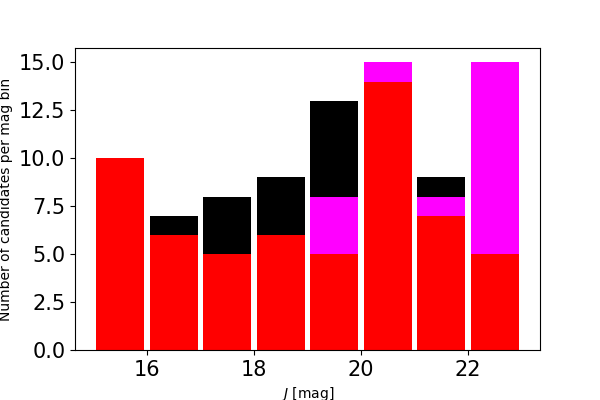
The aim of this subsection is to discuss the shape and form of the USco luminosity and mass functions into the planetary-mass regime. In Table 3, we give the final numbers of candidates before and after rejection of potential photometric non members, equivalent to the luminosity function (Fig. 8). We transform the luminosity function into a mass spectrum, assuming an age of 10 Myr (Pecaut et al. 2012) and the magnitude-mass relation from the BT-Settl model (Baraffe et al. 2015). We also specify the mass range according to the BT-Settl 10 Myr-old isochrone in Table 3. We assumed an age of 10 Myr for USco based on the comparison of these models with the masses derived from eclipsing binaries identified in the association thanks to the Kepler K2 mission (Borucki et al. 2010; Lissauer et al. 2014; Batalha 2014) over the past years (Alonso et al. 2015; Kraus et al. 2015; Lodieu et al. 2015; David et al. 2016b; David et al. 2019). The BT-Settl models at 10 Myr reproduce relatively well the sequence of USco eclipsing binaries in the mass-radius diagram (Lodieu et al. 2020). The age of USco might well be as young as 5 Myr from isochrone fitting of the lowest mass stars (Preibisch & Zinnecker 1999; Preibisch et al. 2001; Song et al. 2012; David et al. 2019) with an upper limit of about 10 Myr (Pecaut et al. 2012).
In Table 3 we observe that the number of objects per bin of magnitudes in the six square degrees is relatively constant over the = 14--20 mag range. We considered Poissonian errors on the luminosity function taking the square root of the number of objects in each column that we need to sum up to obtain the total number of candidates per magnitude bin. This is as a very approximate but recommended practice to estimate the error bars in histograms 22 2 https://docs.astropy.org/en/stable/api/astropy.stats.poisson_conf_interval.html. The last two bins are incomplete because our -band survey is 100% complete down to = 20.5 mag. Typically we find 1.0–1.5 planetary-mass member per square degree in this area of USco, up to two maximum. We observe an increase in the planetary-mass regime if all photometric candidates are bona-fide members. If only the smallest numbers of candidates is confirmed with further follow-ups, the shape of the mass spectrum would rather be flat in the 20–7 MJup range. We can discard a significant decrease in the numbers of members down to 5 MJup, assuming an age of 10 Myr, unless all photometric candidates are rejected in the future. If the age of USco is 5 Myr, the lower mass limit of our survey would be just below 4 MJup. In spite of all uncertainties associated to models at these low masses and young ages as well as the lack of spectroscopic confirmation, star formation processes can form isolated planetary-mass objects down to 5 MJup, consistent with the findings in the solar neighbourhood (Kirkpatrick et al. 2019).
| Rej | no | HSC | dN | Mass range | dN/dM | ||
|---|---|---|---|---|---|---|---|
| mag | M⊙ | ||||||
| 1415 | 10 | 0 | 0 | 0 | 10 (6.8–13.1) | 0.0600–0.0220 | 263 (247–279) |
| 1516 | 7 | 1 | 0 | 0 | 6 (3.5–8.5) | 0.0220–0.0160 | 1000 (968–1032) |
| 1617 | 8 | 3 | 0 | 0 | 5 (2.7–7.2) | 0.0160–0.0120 | 1250 (1214–1285) |
| 1718 | 9 | 3 | 0 | 0 | 6 (3.5–8.5) | 0.0120–0.0095 | 2400 (2351–2449) |
| 1819 | 13 | 5–8 | 0 | 0 | 5–8 (2.7–10.3) | 0.0095–0.0073 | 2242–3587 (2194–3647) |
| 1920 | 9 | 0 | 0–1 | 15 | 14–15 (8.1–20.9) | 0.0073–0.0059 | 10000–10714 (5786-14929) |
| 2021 | 1 | 0 | 1–2 | 15 | 7–8 (1.5–13.5) | 0.0059–0.0045 | 5000–5714 (1071-9643) |
| 2122 | 0 | 0 | 0 | (21)5 | (5–15) (2.9–17.1) | 0.0045–0.0037 | 6250–18750 (3625-21375) |
7 Conclusions and future work
We presented a dedicated photometric search in 6 deg2 in the central region of the USco association to look for the coolest members with a special focus on late-L and T-type candidates. Our survey is the deepest in the association over such large area, between 2 and 1 magnitude deeper in and than any previous study and we are now closer to reach the regime of T dwarfs in USco. The main results of our study are:
-
We identified 10 new candidates fainter than the previously known L7 members confirmed spectroscopically. Their magnitudes are fainter than = 21.7 mag ( 19.5 mag), equivalent to masses below 5 MJup according to evolutionary models at an age of 10 Myr.
-
We highlight two potential T-type member candidates among the 10 faintest sources identified in our deep survey.
-
We derived proper motion confirmation of the brightest member candidates while the accuracy of the astrometry is limited for the newest and faintest candidates.
-
We presented near-infrared spectroscopy of two photometric candidates confirmed them as young L dwarfs, adding credence to their membership. The remaining candidates require optical and/or infrared spectroscopic follow-up.
-
We derive photometric estimates of the luminosity function and mass spectrum in the planetary-mass domain showing no obvious sign of dearth of members down to masses of 5 MJup. Although this analysis is preliminary and requires photometric and spectroscopic follow-ups, there is now growing observational evidence that the star formation processes can form isolated objects with masses below 5 MJup in the field and in young regions.
Acknowledgments
NL was partly funded by the programme AYA2015-69350-C3-2-P from Spanish Ministry of Economy and Competitiveness (MINECO) and acknowledges support from the Agencia Estatal de Investigación del Ministerio de Ciencia e Innovación (AEI-MCINN) under grant PID2019-109522GB-C53. NL has benefited from internal funding from an IAC Severo Ochoa outgoing fellowship for a stay at the Royal Observatory in Edinburgh. We warmly thank the staff at the Royal Observatory Edinburgh and Cambridge Astronomy Survey Unit for their valuable help and support with the data reduction, in particular Mike Read, Rob Blake, Eckhard Sutorius, Mike Irwin, Aybuke Kupcu Yoldas, and Carlos González-Fernańdez.
This research has made use of the Simbad and Vizier (Ochsenbein et al. 2000) databases, operated at the Centre de Données Astronomiques de Strasbourg (CDS), and of NASA’s Astrophysics Data System Bibliographic Services (ADS).
Based on observations collected at the European Organisation for Astronomical Research in the Southern Hemisphere under ESO programme(s) 095.C-0781(A), 089-C.0102(ABC), and 0101.C-0565.
This work is based on programmes GTC4-14A (PI Lodieu) made with the Gran Telescopio Canarias (GTC), operated on the island of La Palma in the Spanish Observatorio del Roque de los Muchachos of the Instituto de Astrofísica de Canarias.
This work is partly based on data collected at Subaru Telescope, which is operated by the National Astronomical Observatory of Japan.
Based on data from the UKIRT Infrared Deep Sky Survey (UKIDSS). The UKIDSS project is defined in Lawrence et al. 2007 and uses the UKIRT Wide Field Camera (Casali et al. 2007, WFCAM;). The photometric system is described in Hewett et al. 2006 and the calibration is described Hodgkin et al. 2009. The pipeline processing and science archive are described in Irwin et al. (2009, in prep) and Hambly et al. 2008.
The Pan-STARRS1 Surveys (PS1) have been made possible through contributions of the Institute for Astronomy, the University of Hawaii, the Pan-STARRS Project Office, the Max-Planck Society and its participating institutes, the Max Planck Institute for Astronomy, Heidelberg and the Max Planck Institute for Extraterrestrial Physics, Garching, The Johns Hopkins University, Durham University, the University of Edinburgh, Queen’s University Belfast, the Harvard-Smithsonian Center for Astrophysics, the Las Cumbres Observatory Global Telescope Network Incorporated, the National Central University of Taiwan, the Space Telescope Science Institute, the National Aeronautics and Space Administration under Grant No. NNX08AR22G issued through the Planetary Science Division of the NASA Science Mission Directorate, the National Science Foundation under Grant No. AST-1238877, the University of Maryland, and Eotvos Lorand University (ELTE).
This publication makes use of data products from the Wide-field Infrared Survey Explorer, which is a joint project of the University of California, Los Angeles, and the Jet Propulsion Laboratory/California Institute of Technology, and NEOWISE, which is a project of the Jet Propulsion Laboratory/California Institute of Technology. WISE and NEOWISE are funded by the National Aeronautics and Space Administration.
John D. Hunter. Matplotlib: A 2D Graphics Environment, Computing in Science & Engineering, 9, 90-95 (2007), DOI:10.1109/MCSE.2007.55 (publisher link) Stefan van der Walt, S. Chris Colbert and Gaël Varoquaux. The NumPy Array: A Structure for Efficient Numerical Computation, Computing in Science & Engineering, 13, 22-30 (2011), DOI:10.1109/MCSE.2011.37 (publisher link) Jones E, Oliphant E, Peterson P, et al. SciPy: Open Source Scientific Tools for Python, 2001-, http://www.scipy.org/ [Online; accessed 2017-10-03].
TOPCAT was initially (2003-2005) developed under the UK Starlink project (1980-2005, R.I.P.). Since then it has been supported by grant PP/D002486/1 from the UK’s Particle Physics and Astronomy Research Council, the VOTech project (from EU FP6), the AstroGrid project (from PPARC/STFC), the AIDA project (from EU FP7), grants ST/H008470/1, ST/I00176X/1, ST/J001414/1 and ST/L002388/1 from the UK’s Science and Technology Facilities Council (STFC), the GAVO project (BMBF Bewilligungsnummer 05A08VHA), the European Space Agency, and the FP7 project GENIUS.
Data Availability
The data underlying this article will be made public to the community through Vizier at the Centre de Données de Strasbourg at http://cdsweb.u-strasbg.fr, and can be accessed with the bibcode or last name of the first author of the paper.
References
- Allers & Liu (2013) Allers K. N., Liu M. C., 2013, ApJ, 772, 79
- Alonso et al. (2015) Alonso R., Deeg H. J., Hoyer S., Lodieu N., Palle E., Sanchis-Ojeda R., 2015, A&A, 584, L8
- Alves de Oliveira et al. (2013) Alves de Oliveira C., Moraux E., Bouvier J., Duchêne G., Bouy H., Maschberger T., Hudelot P., 2013, A&A, 549, A123
- Ardila et al. (2000) Ardila D., Martín E., Basri G., 2000, AJ, 120, 479
- Baraffe et al. (2015) Baraffe I., Homeier D., Allard F., Chabrier G., 2015, A&A, 577, A42
- Barsony et al. (2012) Barsony M., Haisch K. E., Marsh K. A., McCarthy C., 2012, ApJ, 751, 22
- Bastian et al. (2010) Bastian N., Covey K. R., Meyer M. R., 2010, ARA&A, 48, 339
- Batalha (2014) Batalha N. M., 2014, Proceedings of the National Academy of Science, 111, 12647
- Béjar et al. (2008) Béjar V. J. S., Zapatero Osorio M. R., Pérez-Garrido A., Álvarez C., Martín E. L., Rebolo R., Villó-Pérez I., Díaz-Sánchez A., 2008, ApJL, 673, L185
- Best et al. (2017) Best W. M. J., et al., 2017, ApJ, 837, 95
- Boley & Durisen (2010) Boley A. C., Durisen R. H., 2010, ApJ, 724, 618
- Bonnefoy et al. (2014) Bonnefoy M., Chauvin G., Lagrange A.-M., Rojo P., Allard F., Pinte C., Dumas C., Homeier D., 2014, A&A, 562, A127
- Borucki et al. (2010) Borucki W. J., et al., 2010, Science, 327, 977
- Bosch et al. (2018) Bosch J., et al., 2018, PASJ, 70, S5
- Boss (1988) Boss A. P., 1988, ApJ, 331, 370
- Boyd & Whitworth (2005) Boyd D. F. A., Whitworth A. P., 2005, A&A, 430, 1059
- Burgasser et al. (2002) Burgasser A. J., et al., 2002, ApJ, 564, 421
- Burgasser et al. (2003) Burgasser A. J., Kirkpatrick J. D., Liebert J., Burrows A., 2003, ApJ, 594, 510
- Burgasser et al. (2006) Burgasser A. J., Geballe T. R., Leggett S. K., Kirkpatrick J. D., Golimowski D. A., 2006, ApJ, 637, 1067
- Burgess et al. (2009) Burgess A. S. M., Moraux E., Bouvier J., Marmo C., Albert L., Bouy H., 2009, A&A, 508, 823
- Burningham et al. (2010) Burningham B., et al., 2010, MNRAS, 406, 1885
- Burningham et al. (2013) Burningham B., et al., 2013, MNRAS, 433, 457
- Casali et al. (2007) Casali M., Adamson A., Alves de Oliveira C., Almaini O., Burch K., Chuter T., Elliot J., 23 co-authors 2007, A&A, 467, 777
- Cepa et al. (2000) Cepa J., et al., 2000, in M. Iye & A. F. Moorwood ed., Society of Photo-Optical Instrumentation Engineers (SPIE) Conference Series Vol. 4008, Society of Photo-Optical Instrumentation Engineers (SPIE) Conference Series. pp 623–631
- Chambers et al. (2016) Chambers K. C., Magnier E. A., Metcalfe N., 103 co-authors 2016, ApJ,
- Chiang & Chen (2015) Chiang P., Chen W. P., 2015, ApJL, 811, L16
- Chinchilla et al. (2020) Chinchilla P., et al., 2020, A&A, 633, A152
- Cook et al. (2017) Cook N. J., Scholz A., Jayawardhana R., 2017, AJ, 154, 256
- Cross et al. (2012) Cross N. J. G., et al., 2012, A&A, 548, A119
- Cruz et al. (2009) Cruz K. L., Kirkpatrick J. D., Burgasser A. J., 2009, AJ, 137, 3345
- Cutri & et al. (2014) Cutri R. M., et al. 2014, VizieR Online Data Catalog, 2328, 0
- Cutri et al. (2013) Cutri R. M., et al., 2013, Explanatory Supplement to the AllWISE Data Release Products, Explanatory Supplement to the AllWISE Data Release Products
- D’Odorico et al. (2006) D’Odorico S., et al., 2006, in Society of Photo-Optical Instrumentation Engineers (SPIE) Conference Series. , doi:10.1117/12.672969
- Dalton et al. (2006) Dalton G. B., et al., 2006, in Society of Photo-Optical Instrumentation Engineers (SPIE) Conference Series. , doi:10.1117/12.670018
- David et al. (2016a) David T. J., et al., 2016a, Nat, 534, 658
- David et al. (2016b) David T. J., Hillenbrand L. A., Cody A. M., Carpenter J. M., Howard A. W., 2016b, ApJ, 816, 21
- David et al. (2019) David T. J., Hillenbrand L. A., Gillen E., Cody A. M., Howell S. B., Isaacson H. T., Livingston J. H., 2019, ApJ, 872, 161
- Davis (1999) Davis L. E., 1999, in Craine E. R., Crawford D. L., Tucker R. A., eds, Astronomical Society of the Pacific Conference Series Vol. 189, Precision CCD Photometry. p. 35
- Dawson et al. (2011) Dawson P., Scholz A., Ray T. P., 2011, MNRAS, 418, 1231
- Dawson et al. (2013) Dawson P., Scholz A., Ray T. P., Marsh K. A., Wood K., Natta A., Padgett D., Ressler M. E., 2013, MNRAS, 429, 903
- Dawson et al. (2014) Dawson P., Scholz A., Ray T. P., Peterson D. E., Rodgers-Lee D., Geers V., 2014, MNRAS, 442, 1586
- Dupuy & Liu (2012) Dupuy T. J., Liu M. C., 2012, ApJS, 201, 19
- Elias et al. (2006) Elias J. H., Joyce R. R., Liang M., Muller G. P., Hileman E. A., George J. R., 2006, in Ground-based and Airborne Instrumentation for Astronomy. Edited by McLean, Ian S.; Iye, Masanori. Proceedings of the SPIE, Volume 6269, pp. (2006).. , doi:10.1117/12.671817
- Emerson (2001) Emerson J. P., 2001, in R. Clowes, A. Adamson, & G. Bromage ed., Astronomical Society of the Pacific Conference Series Vol. 232, The New Era of Wide Field Astronomy. p. 339
- Emerson et al. (2004) Emerson J. P., Sutherland W. J., McPherson A. M., Craig S. C., Dalton G. B., Ward A. K., 2004, The Messenger, 117, 27
- Faherty et al. (2016) Faherty J. K., et al., 2016, ApJS, 225, 10
- Filippazzo et al. (2015) Filippazzo J. C., Rice E. L., Faherty J., Cruz K. L., Van Gordon M. M., Looper D. L., 2015, ApJ, 810, 158
- Forgan & Rice (2011) Forgan D., Rice K., 2011, MNRAS, 417, 1928
- Furusawa et al. (2018) Furusawa H., et al., 2018, PASJ, 70, S3
- Gagné et al. (2015a) Gagné J., et al., 2015a, ApJS, 219, 33
- Gagné et al. (2015b) Gagné J., Lafrenière D., Doyon R., Malo L., Artigau É., 2015b, ApJ, 798, 73
- Gagné et al. (2017a) Gagné J., et al., 2017a, ApJS, 228, 18
- Gagné et al. (2017b) Gagné J., et al., 2017b, ApJL, 841, L1
- Gaia Collaboration et al. (2018) Gaia Collaboration et al., 2018, A&A, 616, A1
- Gauza et al. (2015) Gauza B., Béjar V. J. S., Pérez-Garrido A., Rosa Zapatero Osorio M., Lodieu N., Rebolo R., Pallé E., Nowak G., 2015, ApJ, 804, 96
- Geballe et al. (2002) Geballe T. R., et al., 2002, ApJ, 564, 466
- Gorlova et al. (2003) Gorlova N. I., Meyer M. R., Rieke G. H., Liebert J., 2003, ApJ, 593, 1074
- Greenfield & White (2006) Greenfield P., White R. L., 2006, in Koekemoer A. M., Goudfrooij P., Dressel L. L., eds, The 2005 HST Calibration Workshop: Hubble After the Transition to Two-Gyro Mode. p. 437
- Haisch et al. (2010) Haisch Jr. K. E., Barsony M., Tinney C., 2010, ApJL, 719, L90
- Hambly et al. (2008) Hambly N. C., et al., 2008, MNRAS, 384, 637
- Hewett et al. (2006) Hewett P. C., Warren S. J., Leggett S. K., Hodgkin S. T., 2006, MNRAS, 367, 454
- Hodgkin et al. (2009) Hodgkin S. T., Irwin M. J., Hewett P. C., Warren S. J., 2009, MNRAS, 394, 675
- Irwin et al. (2004) Irwin M. J., et al., 2004, in Quinn P. J., Bridger A., eds, Optimizing Scientific Return for Astronomy through Information Technologies. Edited by Quinn, Peter J.; Bridger, Alan. Proceedings of the SPIE, Volume 5493, pp. 411-422 (2004).. pp 411–422, doi:10.1117/12.551449
- Iye et al. (2004) Iye M., et al., 2004, PASJ, 56, 381
- Jenness & LSST Data Management Team (2017) Jenness T., LSST Data Management Team 2017, in Lorente N. P. F., Shortridge K., Wayth R., eds, Astronomical Society of the Pacific Conference Series Vol. 512, Astronomical Data Analysis Software and Systems XXV. p. 297 (arXiv:1511.06790)
- Kausch et al. (2015) Kausch W., et al., 2015, A&A, 576, A78
- Kawanomoto et al. (2018) Kawanomoto S., et al., 2018, PASJ, 70, 66
- Kirkpatrick (2005) Kirkpatrick J. D., 2005, ARA&A, 43, 195
- Kirkpatrick et al. (2019) Kirkpatrick J. D., et al., 2019, ApJS, 240, 19
- Komiyama et al. (2018) Komiyama Y., et al., 2018, PASJ, 70, S2
- Kratter et al. (2010) Kratter K. M., Murray-Clay R. A., Youdin A. N., 2010, ApJ, 710, 1375
- Kraus et al. (2008) Kraus A. L., Ireland M. J., Martinache F., Lloyd J. P., 2008, ApJ, 679, 762
- Kraus et al. (2015) Kraus A. L., Cody A. M., Covey K. R., Rizzuto A. C., Mann A. W., Ireland M. J., 2015, ApJ, 807, 3
- Kunkel (1999) Kunkel M., 1999, Ph.D. Thesis, Julius-Maximilians-Universität Würzburg,
- Lafrenière et al. (2010) Lafrenière D., Jayawardhana R., van Kerkwijk M. H., 2010, ApJ, 719, 497
- Lafrenière et al. (2011) Lafrenière D., Jayawardhana R., Janson M., Helling C., Witte S., Hauschildt P., 2011, ApJ, 730, 42
- Lafrenière et al. (2014) Lafrenière D., Jayawardhana R., van Kerkwijk M. H., Brandeker A., Janson M., 2014, ApJ, 785, 47
- Lawrence et al. (2007) Lawrence A., Warren S. J., Almaini O., Edge A. C., Hambly N. C., 17 co-authors 2007, MNRAS, 379, 1599
- Leggett et al. (2000) Leggett S. K., et al., 2000, ApJL, 536, L35
- Lissauer et al. (2014) Lissauer J. J., Dawson R. I., Tremaine S., 2014, Nature, 513, 336
- Liu et al. (2013) Liu M. C., et al., 2013, ApJL, 777, L20
- Liu et al. (2016) Liu M. C., Dupuy T. J., Allers K. N., 2016, ApJ, 833, 96
- Lodieu (2013) Lodieu N., 2013, MNRAS, 431, 3222
- Lodieu et al. (2006) Lodieu N., Hambly N. C., Jameson R. F., 2006, MNRAS, 373, 95
- Lodieu et al. (2007a) Lodieu N., Hambly N. C., Jameson R. F., Hodgkin S. T., Carraro G., Kendall T. R., 2007a, MNRAS, 374, 372
- Lodieu et al. (2007b) Lodieu N., Pinfield D. J., Leggett S. K., Jameson R. F., Mortlock D. J., Warren S. J., co-authors ., 2007b, MNRAS, 379, 1423
- Lodieu et al. (2008) Lodieu N., Hambly N. C., Jameson R. F., Hodgkin S. T., 2008, MNRAS, 383, 1385
- Lodieu et al. (2011a) Lodieu N., Hambly N. C., Dobbie P. D., Cross N. J. G., Christensen L., Martin E. L., Valdivielso L., 2011a, MNRAS, 418, 2604
- Lodieu et al. (2011b) Lodieu N., Dobbie P. D., Hambly N. C., 2011b, A&A, 527, A24
- Lodieu et al. (2013a) Lodieu N., Ivanov V. D., Dobbie P. D., 2013a, MNRAS, 430, 1784
- Lodieu et al. (2013b) Lodieu N., Dobbie P. D., Cross N. J. G., Hambly N. C., Read M. A., Blake R. P., Floyd D. J. E., 2013b, MNRAS, 435, 2474
- Lodieu et al. (2015) Lodieu N., et al., 2015, A&A, 584, A128
- Lodieu et al. (2018a) Lodieu N., Zapatero Osorio M. R., Béjar V. J. S., Peña Ramírez K., 2018a, MNRAS, 473, 2020
- Lodieu et al. (2018b) Lodieu N., Rebolo R., Pérez-Garrido A., 2018b, A&A, 615, L12
- Lodieu et al. (2020) Lodieu N., Paunzen E., Zejda M., 2020, Low-Mass and Sub-stellar Eclipsing Binaries in Stellar Clusters. pp 213–243, doi:10.1007/978-3-030-38509-5_8
- Looper et al. (2007) Looper D. L., Kirkpatrick J. D., Burgasser A. J., 2007, AJ, 134, 1162
- Low & Lynden-Bell (1976) Low C., Lynden-Bell D., 1976, MNRAS, 176, 367
- Lucas & Roche (2000) Lucas P. W., Roche P. F., 2000, MNRAS, 314, 858
- Luhman (2012) Luhman K. L., 2012, ARA&A, 50, 65
- Luhman & Esplin (2020a) Luhman K. L., Esplin T. L., 2020a, AJ, 160, 44
- Luhman & Esplin (2020b) Luhman K. L., Esplin T. L., 2020b, AJ, 160, 44
- Luhman & Mamajek (2012) Luhman K. L., Mamajek E. E., 2012, ApJ, 758, 31
- Luhman et al. (1998) Luhman K. L., Rieke G. H., Lada C. J., Lada E. A., 1998, ApJ, 508, 347
- Luhman et al. (2018) Luhman K. L., Herrmann K. A., Mamajek E. E., Esplin T. L., Pecaut M. J., 2018, AJ, 156, 76
- Manjavacas et al. (2014) Manjavacas E., et al., 2014, A&A, 564, A55
- Mann et al. (2016) Mann A. W., et al., 2016, AJ, 152, 61
- Marocco et al. (2014) Marocco F., et al., 2014, MNRAS, 439, 372
- Martín et al. (1996) Martín E. L., Rebolo R., Zapatero Osorio M. R., 1996, ApJ, 469, 706
- Martín et al. (2004) Martín E. L., Delfosse X., Guieu S., 2004, AJ, 127, 449
- Mauro et al. (2013) Mauro F., Moni Bidin C., Chené A.-N., Geisler D., Alonso-García J., Borissova J., Carraro G., 2013, Revista Mexicana de Astronomía y Astrofísica, 49, 189
- Mayor & Queloz (1995) Mayor M., Queloz D., 1995, Nature, 378, 355
- McGovern et al. (2004) McGovern M. R., Kirkpatrick J. D., McLean I. S., Burgasser A. J., Prato L., Lowrance P. J., 2004, ApJ, 600, 1020
- Miller & Scalo (1979) Miller G. E., Scalo J. M., 1979, ApJS, 41, 513
- Miyazaki et al. (2018) Miyazaki S., et al., 2018, PASJ, 70, S1
- Mužić et al. (2014) Mužić K., Scholz A., Geers V. C., Jayawardhana R., López Martí B., 2014, ApJ, 785, 159
- Nakajima et al. (1995) Nakajima T., Oppenheimer B. R., Kulkarni S. R., Golimowski D. A., Matthews K., Durrance S. T., 1995, Nature, 378, 463
- Ochsenbein et al. (2000) Ochsenbein F., Bauer P., Marcout J., 2000, A&AS, 143, 23
- Peña Ramírez et al. (2011) Peña Ramírez K., Zapatero Osorio M. R., Béjar V. J. S., Rebolo R., Bihain G., 2011, A&A, 532, A42
- Peña Ramírez et al. (2015) Peña Ramírez K., Zapatero Osorio M. R., Béjar V. J. S., 2015, A&A, 574, A118
- Peña Ramírez et al. (2016) Peña Ramírez K., Béjar V. J. S., Zapatero Osorio M. R., 2016, A&A, 586, A157
- Pecaut et al. (2012) Pecaut M. J., Mamajek E. E., Bubar E. J., 2012, ApJ, 746, 154
- Pinfield et al. (2008) Pinfield D. J., Burningham B., Tamura M., Leggett S. K., Lodieu N., Lucas P. W., Mortlock D. J., 28 co-authors 2008, MNRAS, 390, 304
- Preibisch & Zinnecker (1999) Preibisch T., Zinnecker H., 1999, AJ, 117, 2381
- Preibisch & Zinnecker (2002) Preibisch T., Zinnecker H., 2002, AJ, 123, 1613
- Preibisch et al. (1998) Preibisch T., Guenther E., Zinnecker H., Sterzik M., Frink S., Roeser S., 1998, A&A, 333, 619
- Preibisch et al. (2001) Preibisch T., Guenther E., Zinnecker H., 2001, AJ, 121, 1040
- Rebolo et al. (1995) Rebolo R., Zapatero-Osorio M. R., Martín E. L., 1995, Nature, 377, 129
- Rees (1976) Rees M. J., 1976, MNRAS, 176, 483
- Rogers & Wadsley (2012) Rogers P. D., Wadsley J., 2012, MNRAS, 423, 1896
- Salpeter (1955) Salpeter E. E., 1955, ApJ, 121, 161
- Scalo (1986) Scalo J. M., 1986, Fundamentals of Cosmic Physics, 11, 1
- Schlafly et al. (2019) Schlafly E. F., Meisner A. M., Green G. M., 2019, ApJS, 240, 30
- Schmidt et al. (2010) Schmidt S. J., West A. A., Hawley S. L., Pineda J. S., 2010, AJ, 139, 1808
- Schneider et al. (2016) Schneider A. C., Windsor J., Cushing M. C., Kirkpatrick J. D., Wright E. L., 2016, ApJL, 822, L1
- Scholz et al. (2012) Scholz A., Muzic K., Geers V., Bonavita M., Jayawardhana R., Tamura M., 2012, ApJ, 744, 6
- Science Software Branch at STScI (2012) Science Software Branch at STScI 2012, PyRAF: Python alternative for IRAF, Astrophysics Source Code Library (ascl:1207.011)
- Silk (1977) Silk J., 1977, ApJ, 214, 152
- Slesnick et al. (2006) Slesnick C. L., Carpenter J. M., Hillenbrand L. A., 2006, AJ, 131, 3016
- Slesnick et al. (2008) Slesnick C. L., Hillenbrand L. A., Carpenter J. M., 2008, ApJ, 688, 377
- Smette et al. (2015) Smette A., et al., 2015, A&A, 576, A77
- Song et al. (2012) Song I., Zuckerman B., Bessell M. S., 2012, AJ, 144, 8
- Spezzi et al. (2012) Spezzi L., Alves de Oliveira C., Moraux E., Bouvier J., Winston E., Hudelot P., Bouy H., Cuillandre J.-C., 2012, A&A, 545, A105
- Stauffer et al. (1998) Stauffer J. R., Schultz G., Kirkpatrick J. D., 1998, ApJL, 499, 199
- Stetson (1987) Stetson P. B., 1987, PASP, 99, 191
- Tody (1986) Tody D., 1986, in Crawford D. L., ed., Society of Photo-Optical Instrumentation Engineers (SPIE) Conference Series Vol. 627, Society of Photo-Optical Instrumentation Engineers (SPIE) Conference Series. p. 733
- Tody (1993) Tody D., 1993, in Hanisch R. J., Brissenden R. J. V., Barnes J., eds, Astronomical Society of the Pacific Conference Series Vol. 52, Astronomical Data Analysis Software and Systems II. p. 173
- Vernet et al. (2011) Vernet J., et al., 2011, A&A, 536, A105
- Walter et al. (1994) Walter F. M., Vrba F. J., Mathieu R. D., Brown A., Myers P. C., 1994, AJ, 107, 692
- Whitworth & Stamatellos (2006) Whitworth A. P., Stamatellos D., 2006, A&A, 458, 817
- Zapatero Osorio et al. (2000) Zapatero Osorio M. R., Béjar V. J. S., Martín E. L., Rebolo R., Barrado y Navascués D., Bailer-Jones C. A. L., Mundt R., 2000, Science, 290, 103
- Zapatero Osorio et al. (2014a) Zapatero Osorio M. R., Béjar V. J. S., Miles-Páez P. A., Peña Ramírez K., Rebolo R., Pallé E., 2014a, A&A, 568, A6
- Zapatero Osorio et al. (2014b) Zapatero Osorio M. R., et al., 2014b, A&A, 568, A77
- Zapatero Osorio et al. (2014c) Zapatero Osorio M. R., et al., 2014c, A&A, 572, A67
- de Bruijne et al. (1997) de Bruijne J. H. J., Hoogerwerf R., Brown A. G. A., Aguilar L. A., de Zeeuw P. T., 1997, in ESA SP-402: Hipparcos - Venice ’97. pp 575–578
- de Zeeuw et al. (1999) de Zeeuw P. T., Hoogerwerf R., de Bruijne J. H. J., Brown A. G. A., Blaauw A., 1999, AJ, 117, 354
Appendix A Tables with list of candidates
| ID | R.A. | Dec | |||||||||
|---|---|---|---|---|---|---|---|---|---|---|---|
| hh:mm:ss.ss | ∘:′:′′ | mag | mag | mag | mag | mag | mag | mag | mas/yr | mas/yr | |
| 53 | 16:03:50.82 | 21:44:56.7 | 15.0150.010 | 14.3830.018 | 15.7570.010 | 13.8200.004 | — | 13.2260.026 | 13.0290.030 | 44.7 | 4.4 |
| 48 | 16:11:17.11 | 22:17:17.7 | 15.1030.008 | 14.4300.009 | 16.1180.016 | 13.7680.003 | 13.2990.003 | 13.0650.024 | 12.7420.028 | 10.0 | 19.3 |
| 43 | 16:10:30.14 | 23:15:17.1 | 15.1630.009 | 14.3820.007 | 16.1940.007 | 13.8000.003 | 13.2660.003 | 13.0690.025 | 12.7550.026 | 17.9 | 32.3 |
| 34 | 16:10:00.16 | 23:12:19.4 | 15.2180.009 | 14.5780.010 | 16.0930.012 | 13.9710.004 | 13.5600.004 | 13.3910.026 | 13.1050.031 | 38.3 | 13.4 |
| 41 | 16:13:30.33 | 22:44:06.8 | 15.2550.006 | 14.5480.010 | 15.9370.010 | 13.9650.004 | 13.5990.004 | 13.4670.027 | 13.2650.032 | 16.6 | 13.7 |
| 35 | 16:04:40.25 | 22:54:32.6 | 15.2690.007 | 14.4810.019 | 16.4860.013 | 13.7600.003 | 13.2680.003 | 12.8160.025 | 12.1960.025 | 7.3 | 21.6 |
| 46 | 16:13:40.79 | 22:19:46.3 | 15.5700.006 | 14.7070.007 | 16.5800.006 | 14.1400.004 | 13.6530.004 | 13.4160.025 | 13.0580.030 | 2.6 | 25.7 |
| 44 | 16:10:51.78 | 23:33:27.4 | 15.6480.007 | 14.9470.006 | 16.4600.011 | 14.4230.005 | 14.0270.005 | 13.8190.027 | 13.5530.039 | 56.9 | 97.7 |
| 50 | 16:12:53.13 | 21:46:27.4 | 15.6880.006 | 14.9770.020 | 16.3350.010 | 14.5530.006 | 14.1740.006 | 13.9750.027 | 13.7880.039 | 27.0 | 1.4 |
| 32 | 16:08:30.49 | 23:35:11.3 | 15.7530.010 | 14.8500.006 | 16.9290.011 | 14.3110.005 | 13.7460.005 | 13.3600.026 | 12.8410.029 | 5.4 | 17.8 |
| 51 | 16:07:23.81 | 22:11:02.2 | 16.0410.007 | 15.1330.009 | 17.2690.013 | 14.5650.006 | 13.9890.006 | 13.7070.027 | 13.3930.033 | 3.5 | 29.5 |
| 38 | 16:05:01.90 | 23:21:30.5 | 16.0680.012 | 15.1480.007 | 17.2260.010 | 14.5060.004 | 13.9680.005 | 13.7780.028 | 13.3730.035 | 19.1 | 18.4 |
| 33 | 16:09:05.67 | 22:45:16.9 | 16.0900.006 | 15.2040.009 | 17.3210.014 | 14.5720.006 | 14.0140.005 | 13.8170.026 | 13.4590.033 | 3.0 | 9.1 |
| 55 | 16:04:42.11 | 22:34:11.1 | 16.2280.010 | 15.4160.012 | 17.1480.007 | 14.8120.007 | 14.3620.007 | 14.1720.029 | 14.0130.046 | 13.1 | 65.5 |
| 31 | 16:08:28.46 | 23:15:10.6 | 16.4430.007 | 15.4900.009 | 17.6760.008 | 14.7950.007 | 14.1380.006 | 13.7650.027 | 13.1790.030 | 15.8 | 28.0 |
| 54 | 16:06:02.58 | 22:02:49.9 | 16.5940.007 | 15.5540.011 | 17.9160.020 | 14.9530.007 | 14.3400.007 | 14.0970.028 | 13.7000.041 | 33.0 | 7.8 |
| 56 | 16:06:03.75 | 22:19:30.2 | 16.9140.013 | 15.8650.015 | 18.3020.018 | 15.1120.008 | 14.4400.007 | 13.9320.030 | 13.3070.033 | 3.7 | 16.4 |
| 52 | 16:08:18.42 | 22:32:25.2 | 17.1430.011 | 16.1400.012 | 18.5410.012 | 15.3870.011 | 14.6760.010 | 14.3310.031 | 13.9820.046 | 4.1 | 7.3 |
| 49 | 16:13:01.39 | 21:42:54.8 | 17.3050.009 | 16.3900.018 | 18.4270.010 | 15.6310.014 | 15.0700.013 | 14.8590.035 | 14.7380.069 | 18.1 | 12.7 |
| 37 | 16:04:16.18 | 23:26:29.9 | 17.3230.013 | 16.4340.007 | 18.6850.006 | 15.6570.012 | 15.0430.013 | 14.6690.033 | 14.3190.056 | 49.7 | 18.9 |
| 47 | 16:10:38.36 | 21:51:47.0 | 17.4640.005 | 16.3160.020 | 18.8990.017 | 15.4730.012 | 14.7810.009 | 14.3500.031 | 13.8070.040 | 5.6 | 30.6 |
| 45 | 16:16:10.64 | 21:51:24.5 | 17.6460.005 | 16.5550.009 | 18.8310.008 | 15.9950.020 | 15.4510.018 | — | — | 12.6 | 26.7 |
| 29 | 16:07:14.78 | 23:21:01.4 | 17.6710.008 | 16.5810.004 | 19.1240.008 | 15.8070.016 | 15.0590.014 | 14.4640.033 | 13.8120.041 | 5.5 | 24.1 |
| 30 | 16:07:37.97 | 22:42:47.2 | 17.8220.011 | 16.8190.008 | 19.4120.024 | 16.0910.020 | 15.4500.019 | 15.0980.039 | 14.7430.075 | 1.1 | 12.1 |
| 36 | 16:06:09.04 | 23:38:11.6 | 18.0350.006 | 16.9110.008 | 19.5010.012 | 16.2470.020 | 15.5640.020 | 15.1760.044 | 14.8950.085 | 7.2 | 13.0 |
| 39 | 16:04:36.56 | 23:25:24.1 | 18.2560.023 | 17.1450.020 | 19.6640.018 | 16.3480.021 | 15.6710.024 | — | — | 12.5 | 27.8 |
| 57 | 16:05:12.06 | 21:45:28.4 | 18.3580.010 | 17.0800.010 | 19.7920.012 | 16.4030.024 | 15.6450.020 | — | — | 11.1 | 23.0 |
| 40 | 16:14:20.44 | 22:59:52.5 | 18.4630.006 | 17.4430.013 | 19.6150.016 | 16.7530.034 | 16.3130.044 | 16.2680.086 | 16.5850.365 | 44.6 | 59.9 |
| 42 | 16:14:22.56 | 23:31:17.9 | 18.6580.009 | 17.4420.012 | 20.2240.023 | 16.8300.034 | 16.0800.031 | — | — | 10.3 | 20.8 |
| 8 | 16:14:02.87 | 23:14:42.7 | 19.0940.008 | 17.8790.009 | 20.3290.012 | 17.2150.051 | 16.6060.053 | 16.1820.074 | 15.8600.169 | 6.2 | 7.6 |
| 9 | 16:15:32.35 | 22:59:51.0 | 19.1090.007 | 17.8780.009 | 20.3960.020 | 17.2400.056 | 16.5640.058 | 15.8220.055 | 15.6390.146 | 20.0 | 29.1 |
| 27 | 16:06:01.43 | 22:06:16.3 | 19.1930.008 | 18.0370.009 | 20.4010.032 | 17.3190.055 | 16.7920.059 | 16.4890.092 | 16.1620.227 | 23.3 | 10.5 |
| 21 | 16:07:55.40 | 22:33:52.5 | 19.2230.015 | 18.0550.010 | 20.2860.028 | 17.5220.070 | 16.8600.065 | — | — | 33.4 | 4.8 |
| 25 | 16:09:56.36 | 22:22:45.9 | 19.2780.016 | 17.8710.016 | 20.5890.016 | 16.9150.039 | 16.2210.035 | — | — | 4.5 | 37.6 |
| 23 | 16:09:06.61 | 21:41:05.3 | 19.2930.005 | 18.1280.018 | 20.6280.021 | 17.3980.067 | 16.7580.059 | 16.6870.106 | 16.1230.217 | 25.4 | 3.0 |
| 20 | 16:07:31.61 | 21:46:54.5 | 19.5230.009 | 18.0000.013 | 20.9380.034 | 17.0040.046 | 16.2000.034 | 15.1470.040 | 14.5960.062 | 6.2 | 12.5 |
| 24 | 16:09:18.67 | 22:29:23.9 | 19.5340.017 | 17.9480.009 | 20.7860.013 | 16.9740.041 | 16.1390.033 | 15.5390.051 | 15.3170.114 | 33.2 | 16.1 |
| 4 | 16:04:13.03 | 22:41:03.4 | 19.5530.027 | 18.1930.020 | 20.8000.050 | 17.2350.054 | 16.4160.042 | 15.4620.049 | 15.2540.105 | 17.0 | 7.9 |
| 12 | 16:13:34.65 | 21:36:20.3 | 19.6440.008 | 18.2070.017 | 20.9180.017 | 17.1110.045 | 16.3850.039 | 15.7440.053 | 15.3690.120 | 34.4 | 11.5 |
| 14 | 16:14:07.56 | 22:11:52.3 | 19.7050.009 | 18.2240.016 | 21.1050.020 | 17.3860.070 | 16.3840.049 | 15.5700.051 | 15.2900.105 | 3.4 | 23.0 |
| 17 | 16:11:10.15 | 21:45:16.9 | 19.7450.017 | 18.4100.027 | 21.9380.144 | 17.3030.057 | 16.4410.040 | — | — | 0.6 | 30.4 |
| 19 | 16:11:44.37 | 22:15:44.7 | 19.8220.008 | 17.9090.010 | 20.7300.027 | 16.8710.044 | 15.8980.030 | 15.3030.045 | 14.7260.070 | 1.3 | 16.9 |
| 3 | 16:08:43.43 | 22:45:16.2 | 19.8500.018 | 18.3170.021 | 21.1620.041 | 17.1920.056 | 16.2990.040 | 15.4120.045 | 14.6700.069 | 4.8 | 6.0 |
| 28 | 16:04:20.42 | 21:34:53.1 | 19.8990.012 | 18.4480.012 | 21.1130.022 | 17.4320.061 | 16.4980.045 | 15.6950.051 | 15.3320.110 | 27.4 | 14.5 |
| 26 | 16:08:42.37 | 22:23:26.3 | 19.9090.012 | 18.6250.020 | 21.1690.025 | 17.8700.094 | 17.2450.091 | 16.9590.149 | 16.1180.235 | 8.4 | 60.5 |
| 18 | 16:11:10.83 | 22:03:47.6 | 20.0810.011 | 18.8570.012 | 21.2600.027 | 18.0470.118 | 17.3250.092 | — | — | 16.4 | 23.3 |
| 16 | 16:11:05.28 | 22:22:57.4 | 20.4660.016 | 19.1490.019 | 21.9530.046 | 18.4610.192 | 17.3130.109 | — | — | 8.3 | 11.5 |
| 5 | 16:04:31.51 | 23:13:04.4 | 20.5490.013 | 19.1230.021 | 21.9050.046 | 18.4640.152 | 17.6290.140 | — | — | 31.9 | 6.9 |
| 13 | 16:15:15.22 | 21:48:46.6 | 20.9220.015 | 19.5150.029 | 22.2870.051 | — | — | — | — | 21.7 | 7.0 |
| 15 | 16:15:12.70 | 22:29:49.2 | 20.9430.019 | 19.2640.025 | 22.3070.071 | 18.1670.142 | 17.0650.087 | 16.5290.100 | 15.7290.156 | 7.9 | 1.4 |
| 22 | 16:08:34.28 | 21:48:04.9 | 20.9840.015 | 19.3460.039 | 22.2690.094 | — | 17.7990.152 | 17.0220.153 | 16.9390.476 | 10.0 | 3.0 |
| 11 | 16:12:37.84 | 22:51:12.9 | 21.7810.038 | 19.5040.039 | 22.2590.062 | — | — | — | — | 83.9 | 564.2 |
| 6 | 16:05:17.84 | 23:35:51.9 | 21.8240.019 | 18.0640.029 | 21.9600.055 | — | — | — | — | 259.8 | 17.4 |
| 1 | 16:09:29.08 | 23:40:48.2 | 21.9090.136 | 19.3360.040 | 22.7000.083 | 18.3680.168 | — | — | — | 486.5 | 47.5 |
| 7 | 16:04:04.50 | 23:21:31.0 | 22.1640.049 | 19.6880.050 | 22.4960.082 | — | — | — | — | 155.2 | 350.4 |
| 10 | 16:15:04.04 | 22:40:13.3 | 22.1990.097 | 19.5560.022 | 22.6340.084 | 18.4300.170 | — | — | — | 377.2 | 356.6 |
| 2 | 16:10:03.24 | 23:18:11.8 | 22.7560.078 | 20.4440.068 | 23.2960.159 | — | — | 17.5000.199 | 16.5190.000 | 564.3 | 43.1 |
| ID | R.A. | Dec | ||||
|---|---|---|---|---|---|---|
| hh:mm:ss.ss | ∘:′:′′ | mag | mag | mas/yr | mas/yr | |
| candYJ_VISTA_101 | 16:09:13.79 | 23:35:46.9 | 22.2270.166 | 20.2470.089 | 149.5 | 109.0 |
| candYJ_VISTA_102 | 16:04:46.67 | 22:52:41.4 | 22.4590.085 | 20.3670.083 | 272.8 | 65.1 |
| candYJ_VISTA_103 | 16:06:26.99 | 22:50:00.6 | 22.1830.129 | 20.0860.058 | 352.1 | 448.9 |
| candYJ_VISTA_104 | 16:14:41.41 | 22:16:29.8 | 22.6690.070 | 19.5690.046 | 330.8 | 340.0 |
| ID | R.A. | Dec | ||||
|---|---|---|---|---|---|---|
| hh:mm:ss.ss | ∘:′:′′ | mag | mag | mag | ||
| candYJ_HSC_1005 | 16:12:03.71 | 22:35:09.4 | 23.8790.064 | 22.3180.077 | 20.5360.081 | |
| candYJ_HSC_1002 | 16:13:59.13 | 22:12:36.8 | 24.1920.100 | 23.0820.122 | 21.1760.114 | |
| candYJ_HSC_1001 | 16:14:14.47 | 23:12:36.7 | 24.2660.096 | 22.9610.171 | 21.0820.107 | |
| candYJ_HSC_1003 | 16:14:41.41 | 22:16:29.8 | 22.9590.025 | 22.6690.070 | 19.5690.046 | |
| candYJ_HSC_1004 | 16:15:32.45 | 22:11:05.4 | 23.9940.073 | 22.9640.126 | 21.2020.126 | |