The AAA framework for linear dynamical systems with quadratic output \shortdate
Data-driven modeling of linear dynamical systems with quadratic output in the AAA framework
Abstract
We extend the AAA (Adaptive-Antoulas-Anderson) algorithm to develop a data-driven modeling framework for linear systems with quadratic output (LQO). Such systems are characterized by two transfer functions: one corresponding to the linear part of the output and another one to the quadratic part. We first establish the joint barycentric representations and the interpolation theory for the two transfer functions of LQO systems. This analysis leads to the proposed AAA-LQO algorithm. We show that by interpolating the transfer function values on a subset of samples together with imposing a least-squares minimization on the rest, we construct reliable data-driven LQO models. Two numerical test cases illustrate the efficiency of the proposed method.
keywords
data-driven modeling, nonlinear dynamics, rational approximation, barycentric form, interpolation.1 Introduction
Model order reduction (MOR) is used to approximate large-scale dynamical systems with smaller ones that ideally have similar response characteristics to the original one. This has been an active research area and many approaches to MOR have been proposed. We refer the reader to [1, 6, 3, 24, 8, 26] and the references therein for an overview of MOR methods for both linear and nonlinear dynamical systems.
MOR, as the name implies, assumes access to a full order model to be reduced; in most cases, in the form of a state-space formulation obtained via, e.g., a spatial discretization of the underlying partial differential equations. Then, the reduced order quantities are computed via an explicit projection of the full-order quantities. However, in some cases, access to full order dynamics is not available. Instead, one has access to a collection of input/output measurements. In this case, the goal is to construct the approximation directly from data, which we refer to as data-driven modeling. This is the framework we consider in this paper.
Specifically, we focus on data-driven modeling of linear dynamical systems with quadratic output (LQO). In our formulation, data correspond to frequency domain samples of the input/output mapping of the underlying LQO system, in the form of samples of its two transfer functions; the first transfer function being a single-variable one and the second a bivariate one. For this data set, the proposed framework first develops the barycentric rational interpolation theory for LQO systems to interpolate a subset of the data and and then extends the AAA algorithm [20] to this setting by minimizing a least-square measure in the remaining data.
We note that system identification of general nonlinear systems has been a popular topic. In particular, we mention here the special case of identifying linear systems with nonlinear output or input functions, e.g., the so-called Wiener [30] and Hammerstein models, respectively. Significant effort has been allocated for identification of such models; see, e.g., [16], [12] and the references therein. Nevertheless, the methods previously mentioned are based in the time domain, while in this paper we focus on frequency domain data. We point out that the frequency-data based Loewner framework was recently extended to identifying Hammerstein models in [18].
The rest of the paper is organized as follows: We discuss LQO systems and their transfer functions in Section 2, followed by a review of barycentric rational approximation and the AAA algorithm in Section 3. Next, we develop the theory for barycentric representation and multivariate interpolation for LQO systems in Section 4. Based on this analysis, in Section 5, we present the proposed algorithm, AAA-LQO, for data-driven modeling of LQO systems. The numerical experiments are given in Section 6 followed by the conclusions in Section 7.
2 Linear systems with quadratic output
In state-space form, linear dynamical systems with quadratic output (LQO systems) are described as
| (1) |
where , , , and the symbol denotes the Kronecker product, i.e., for the vector , we have
The quadratic part of the output in eq. 1, , can be rewritten as with and where vec denotes the vectorization operation. In some cases, in eq. 1 we have , and thus the output has only the quadratic term.
Several projection-based MOR methodologies have been already proposed for LQO systems. More precisely, balanced truncation-type methods were considered in [28, 23, 7], while interpolation-based methods were used in [29, 14]. All these methods are intrusive, meaning that, they explicitly work with the state-space matrices and in eq. 1.
The main goal of this work is to develop a data-driven modeling framework for LQO systems where only input-output measurements, in the form of transfer function evaluations, are needed as opposed to the internal state-space representation. Therefore, our first goal is to derive transfer functions for this special class of dynamical systems.
2.1 The transfer functions of LQO systems
Many classes of nonlinear systems can be represented in the time domain by generalized kernels as presented in the classical Wiener or Volterra series representations. Generically, infinite number of kernels appear in such series, corresponding to each homogeneous subsystem. For more details we refer the reader to [30, 25]
For the LQO system eq. 1, the nonlinearity is present in the state-to-output equation only and one can write the input-output mapping of the system in the frequency domain using two transfer functions
- 1.
one corresponding to the linear part of the output, i.e., ;
- 2.
one corresponding to the quadratic part of the output, i.e., .
These transfer functions were recently derived in [14] using their time-domain representations. In the next result, we introduce and re-derive them for the completeness of the paper and to illustrate to the reader how they naturally appear.
Lemma 1.
Consider the LQO system in eq. 1 with . Let the input be a sum of the harmonic terms, i.e.,
| (2) |
and . Then, the output is given by
| (3) |
where
| (4) |
is the single-variable rational transfer function corresponding to and
| (5) |
is the two-variable rational transfer function corresponding to with denoting the identity matrix of size .
Proof.
For the input in eq. 2 with , the solution of the linear state-equation in eq. 1 in steady-state can be written as a sum of scaled complex exponential functions as
| (6) |
where . Substituting eq. 6 into the output equation of eq. 1, we obtain
| (7) | ||||
Substituting back into the last equation yields the desired resulteq. 3 with and as defined in eq. 4 and eq. 5. ∎
Lemma 1 shows that the LQO system eq. 1 is characterized by two transfer functions, namely (corresponding to the linear component in the output) and (corresponding to the quadratic linear in the output). As in the classical linear case, is a rational function in single variable. On the other hand, is also a rational function, but of two variables. These two transfer functions that fully describe the LQO system eq. 1 will play the fundamental role in our analysis to extend barycentric interpolation and AAA to the LQO setting. Before we establish the theory for LQO systems, we will briefly review the AAA algorithm for linear systems in Section 3.
Remark 1.
In the proposed framework, we will require sampling the two transfer functions and . As it is shown in Lemma 1, this could be achieved by exciting the system (as a black box) with purely oscillatory control inputs and measuring the outputs, and performing a Fourier transformation. For more details on such procedures in similar settings, we refer the reader to [17]. We also note that [27] examines systems described by two time-domain kernels together with their Fourier transformations (deemed as transfer functions) and their measurements. Even though no explicit representation of these functions are considered in terms of a state-space realization, those ideas also equally apply to sample and .
Remark 2.
Note that in the special case for which it holds that , we obtain where is a scalar. Therefore, in this case the output is a quadratic polynomial in the linear output and the LQO model can be interpreted as a Wiener model [30]. However, our focus here is on the general case of LQO systems without this special case.
3 Barycentric rational approximation for linear systems and the AAA algorithm
For an underlying function , e.g., transfer function of a single-input/single-output (SISO) linear dynamical system, assume the following set of measurements:
| (8) |
Partition the sampling points into two disjoint sets:
| (9) |
We will clarify later how this partitioning is chosen. Based on eq. 9, define the sampled values
and the corresponding data sets
| (12) |
Define the rational function in barycentric form [9], a numerically stable representation of rational functions11 1 With the addition of to the denominator, we guarantee that is a strictly proper rational function with a numerator degree and the denominator degree . This is done in the anticipation of the dynamical system in eq. 1 we aim to approximate where there will be no direct input-to-output mapping. This is not a restriction, and the numerator and denominator degrees can be chosen in a different way [9, 20].:
| (13) |
where are the sampling (support) points and the weights are to be determined. By construction, the degree-() rational function in eq. 13 is a rational interpolant at the support point set , i.e.,
| (14) |
assuming . Then, the freedom in choosing the weights can be used to match the remaining the data in an appropriate measure.
Assuming enough degrees of freedom, [2] chooses the weights to enforce interpolation of as well, by computing the null space of the corresponding divided difference matrix, thus obtaining a degree-() rational function interpolating the full data eq. 8. We skip the details for the conditions to guarantee the existence and uniqueness of such a rational interpolant and refer the reader to [2, 3] for details.
The AAA (Adaptive-Antoulas-Anderson) algorithm [20], on the other hand, elegantly combines interpolation and least-squares (LS) fitting. In the barycentric form eq. 13, which interpolates the data by construction, AAA chooses the weights to minimize a LS error over the data . Note that the LS problem over is nonlinear in the weights since these weights appear in the denominator of as well. AAA solves a relaxed linearized LS problem instead. For a sampling point in the set , AAA uses the linearization
| (15) |
leading to the linearized LS problem
| (16) |
AAA is an iterative algorithm and builds the partitioning eq. 9 using a greedy search. Assume in step , AAA has the rational approximant as in eq. 13 corresponding to the partitioning eq. 9 where the weights are selected by solving eq. 16. AAA updates eq. 9 via a greedy search by finding for which the error is the largest. This sampling point is, then, added to the interpolation set , the barycentric rational approximant in eq. 13 is updated accordingly (it has one higher degree now), and the new weights are computed, as before, solving the linearized LS problem. The procedure is repeated until either a desired order or an error tolerance is obtained. For further details, we refer the reader to the original source [20]. The AAA algorithm proved very flexible and effective, and has been employed in various applications such as rational approximation over disconnected domains [20], solving nonlinear eigenvalue problems [19], modeling of parametrized dynamics [10], and approximation of matrix-valued functions [15].
4 Barycentric representations for LQO systems
To develop interpolating barycentric forms for and , we first need to specify the data corresponding to the underlying the LQO system . The first transfer function of is a regular single-variable rational function and, as in Section 3, we sample at distinct points to obtain the data set
| (17) |
The second transfer function , on the other hand, is a function of two-variables. Therefore, in agreement with the data eq. 17, we will sample at the corresponding rectangular grid: for ,
| (18) |
Partition the full set of sampling points into two disjoint sets
| (19) |
and define the sampled values (measurements):
| (20) |
and
| (21) |
Then, the goal is to a construct a data-driven LQO system directly from its samples without access access to internal dynamics of . The partition eq. 19 and the error measure used in approximating the data will be clarified later. First we will show how the data in eq. 17 and eq. 18 can be used to develop barycentric-like representations corresponding to a reduced LQO system. We will use the notation to denote the rational approximation to and to .
Proposition 1.
Proof.
The fact that is an interpolating rational function for the data eq. 20 is just a restatement of eq. 14 for completeness. To prove eq. 24, we will use the Sherman-Morrison formula [13]: Let be an invertible and be such that Then,
| (25) |
From eq. 23 and eq. 24, we have
| (26) |
To simplify the notation, let . Then, applying the Sherman-Morrison formula to the middle term in eq. 26 with , , and , we obtain
| (27) |
Since is diagonal,
Then, using the definitions of and in eq. 23, we obtain
| (28) |
Substituting these last two equalities into eq. 27 yields eq. 24. ∎
We note that state-space realizations for rational functions are unique up to a similarity transformations. For other equivalent state-space representations of a barycentric form, we refer the reader to, e.g., [5, 19].
Given the samples of ( the data in eq. 20) of the LQO system eq. 1, Proposition 1 constructs the linear part of the data-driven LQO model, directly from these samples. What we need to achieve next is to use the samples (data in eq. 21) to construct a two-variable rational function in a barycentric-like form corresponding to the quadratic part of the data-driven LQO model. However, cannot be constructed independently from . Once is constructed, we should be able to interpret and as the linear and quadratic transfer functions of a single LQO system. This is the precise reason that we cannot simply view as an independent two-variable rational function and use the classical multivariate barycentric form [4, 3]. Therefore, needs to have the form
where and are the same matrices from eq. 23 used in modeling and is the (quadratic) free variable that will incorporate to model the new data eq. 21. The next result achieves this goal.
Theorem 1.
Assume the set-up in Proposition 1. Further assume that the samples in eq. 18 are given. Define, the two-variable function in a barycentric-like form:
| (29) |
Then, interpolates the data eq. 21, i.e.,
| (30) |
Define and using
| (31) | ||||
| (32) |
Then, has the state-space form
| (33) |
Proof.
To prove the interpolation property eq. 30 of the barycentric representation eq. 29, inspired by the linear case, we start by introducing various polynomials in one or two variables:
| (34) | ||||
for . Multiply both the numerator and denominator of in (29) with to obtain
| (35) |
with
| (36) |
Then, evaluate at and to obtain
To prove eq. 33, we first note that
where we used the fact
as shown in deriving eq. 27. Since diagonal, we have
Then, using the definition of in eq. 32 together with the second formula in eq. 28, we obtain
| (37) | ||||
which concludes the proof. ∎
The next result follows from Propositions 1 and 1.
Corollary 1.
Assume the set-up in Propositions 1 and 1. Then, interpolating rational functions and together correspond to an interpolatory LQO model
| (38) |
In others words, the first (linear) transfer function of is and its second transfer function is .
Recall the partitioning of the sampling points in (19). In Theorem 1, we have shown that interpolates over the sampling set . What is the value of over the mixed sampling sets and ? Even though we do not enforce interpolation over these sets, in Section 5 we will need a closed-form expression for the value of over and . The next lemma establishes these results.
Lemma 2.
Proof.
Proof is given in Appendix A. ∎
5 Proposed framework for data-driven modeling of LQO systems
Section 4 established the necessary ingredients to extend AAA to LQO systems. Given the measurements eq. 17 and eq. 18, Propositions 1 and 1 show how to construct the barycentric forms and interpolating this data in accordance with the partitioning eq. 19. Furthermore, Corollary 1 states that and together correspond to an interpolatory LQO system. Based on these results, in this section we will fully develop the AAA framework for LQO systems. The resulting algorithm will be denoted by AAA-LQO.
AAA-LQO will be an iterative algorithm, adding one degree of freedom to the current data-driven LQO model in every iteration step. In the th step, and will correspond to a data-driven order- LQO model for the partitioning of the sampling points in eq. 19. First, for this current partitioning, in Section 5.1, we introduce a LS error measure that will be used to choose the barycentric weights appearing in the definitions of and in eq. 22 and eq. 29. Then, in Section 5.2 we establish a greedy search procedure for updating the partitioning eq. 19. The algorithm will then continue with the LS minimization for the updated partitioning at the th step to construct and . AAA-LQO will terminate after a desired error criterion is met or a maximum allowed order is achieved as explained in Section 5.3.
Even though Section 5.1 investigates the LS problem in the the of AAA-LQO, to simplify the notation, we drop the superscript and use and instead. However, they should be understood as the approximants in the th step. We will reintroduce the superscript in Section 5.2.
5.1 A combined LS measure for computing the barycentric weights for the current partition
For the full LQO data eq. 17 and eq. 18, we recall (and repeat) the partitioning of the sampling points as in eq. 19:
| (40) |
Then, interpolates over (i.e., it interpolates the data eq. 20) and interpolates over (i.e., it interpolates the data eq. 21). Also recall that together, and correspond to a LQO system. The only remaining degrees of freedom in defining and , and thus the corresponding LQO system are the barycentric weights . We will choose those weights to minimize an appropriate error measure in the uninterpolated data corresponding to the sampling points . We first introduce the notation for these uninterpolated values22 2 Since the evaluation of the uninterpolated values occur over three different sets, namely , , and , we use a superscript to distinguish them. Recall that the interpolated values are over only and thus the superscript notation is avoided for .:
| (41) | |||
| (42) | |||
| (43) | |||
| (44) |
We denote with the vector of weights to be determined, as
A reasonable error measure to minimize is the LS distance in the uninterpolated data, leading to the minimization problem
| (45) |
where
| (46) | ||||
| (47) | ||||
| (48) | ||||
| (49) |
As in the original AAA for linear dynamical systems, the LS problem eq. 45 is nonlinear in for LQO systems. The formulation is more complicated here due to the additional term. To resolve this numerical difficulty, we will employ a strategy, similar to the lineraziation step in eq. 15, and solve a relaxed optimization problem. However, the resulting LS problem in our case will still be nonlinear, yet much easier to solve than eq. 45. In the end, we will tackle the original nonlinear LS problem eq. 45 by solving a sequence of quadratic LS problems. We note that in eq. 46-eq. 49, we scale every error term with the number of data points in it.
5.1.1 Quadraticized LS problem in Step
In this section, we show how to relax the each term, , in the nonlinear LS problem eq. 45. The resulting problem will then constitute a crucial component in the proposed iterative algorithm (Section 5.3).
Linearizing :
Note that the th term of in eq. 46, namely , is the same as the term in eq. 15 appearing in AAA. This is natural since corresponds to the linear part of the LQO system. Therefore, we can linearize similar to eq. 15. Write as , as defined in (22). Then, the th term in eq. 46 is linearized as
| (50) |
Substituting and from the definition of in eq. 22 into eq. 50, one obtains
| (51) |
For a matrix , let denote its th entry. Similarly, for a vector , let denote its th entry. Then, define the Loewner matrix with
| (52) |
and the vector with . Then,
Therefore, the term in eq. 46 will be relaxed to
| (53) |
Linearizing and :
Now we extend the linearization strategy used in , which only involved the single-variable function , to the error terms and , which involve . The closed-form expressions for and we derived in Lemma 2 will prove fundamental in achieving these goals.
We start with . Write as in eq. 35. Then, the linearizing the term in (47) means
| (54) |
We substitute and from eq. 39 into eq. 54 to obtain
| (55) |
Define the indexing variable and let be the vector defined such that
| (56) |
Define the Loewner matrix with entries
| (57) |
for , and . Then, using (57) and (56) in (55), we obtain
yielding the linearization of :
| (58) |
Using similar arguments and the explicit formula for the expression in eq. 39, the term in eq. 48 is linearized to
| (59) |
where the Loewner matrix and the vector are defined as
with , , and .
Quadraticizing the term:
In this section we show how to relax the remaining term, , in the minimization problem eq. 45. Note that this term includes ; i.e., evaluated over . As we stated earlier, unlike ( over ) or ( over ), the numerator and denominator of the quantity is quadratic in the weights . Therefore, relaxing the th term in via multiplying it out with its denominator, will not yield a linear term, but rather a quadratic, i.e., even the relaxed problem cannot be solved as a linear LS problem. This is what we establish next.
Similar to (54), relax the th term in (49) using
| (60) |
Using (37), we obtain
| (61) |
Inserting and from (61) into (60) and re-arranging the terms yields
| (62) |
Note that the expression in (62) is quadratic in , as anticipated.
As we did for the , and , to express the resulting expression more compactly in matrix form, we introduce the (2D) Loewner matrix as
| (63) |
where and with and . Then, the th entry of the vector is
| (64) |
thus recovering the first sum in (62). Next, introduce the matrices such that for ,
| (65) |
Using and in eq. 65, the last two sums in (62) can be compactly written as
| (66) |
Define . Then using eq. 65, we write
| (67) |
Insert (63) and (67) into (61) obtain
| (68) |
where is the vector defined as
| (69) |
with as before and . The expression (68) yields the final relaxation of :
| (70) |
5.1.2 Solving the optimization problem in Step
Combining the relaxations , , , and as given in (53), (58), (59), and (70), at the th step of the algorithm, we need to solve the quadraticized minimization problem
| (71) | |||
where
| (72) |
Note that due to the last term, the optimization problem (71) is no longer a linear LS problem, nevertheless can be solved efficiently. One can explicitly compute the gradient (and Hessian) of the cost function and can apply a well-established (quasi)-Newton formulation [21]. If we were to have a one-step algorithm whose solution is given by (71), one would employ these techniques. However, note that solving (71) is only one step of our proposed iterative algorithm. Hence, as the iteration continues (and increases) the vector (and the data-partition) will be updated and the new optimization problem with a larger-dimension needs to be solved. Therefore, we will approximately solve (71) in every step.
One can obtain an approximate solution to (71) in various ways. In our formulation, we will first solve part of the problem (71) that can be written as a linear least-squares problem in , namely
| (73) |
The optimization problem (73) is a classical linear least-squares problem:
| (74) |
Using , we further relax the last term in eq. 71 as
| (75) |
Using , we rewrite (75) as
| (76) |
where the matrix is defined as follows
| (77) |
Then, using eq. 76 in place of the last term in (71), we obtain a minimization problem that is now a linear LS problem. Thus, the solution to our final approximation to (71) is given by
| (78) |
Therefore, in the th step of AAA-LQO, the optimization problem (45) is relaxed and the solution of this relaxed problem (the weights) is given by (78). The algorithms proceeds with the updated weights as we discuss next.
5.2 Partition update via the greedy selection
Given the partition (40) in the Step of the algorithm, Section 5.1 showed how to choose the barycentric weights to minimize a joint LS measure over the uninterpolated data set. The only remaining component of the proposed approach is, then, to choose the next support point and update the data partition (40) (so that we repeat Section 5.1 for the updated partition until a desired tolerance achieved.) In other words, we will move one sampling point from the LS set to the interpolation set . Which point to move from to will be done in a greedy manner. To emphasize the iterative nature of the overall algorithm, at this Step of the algorithm, we will denote by and the two transfer functions of the current LQO approximant. (Note that we dropped the superscript in Section 5.1 to simplify the notation there.)
We start by defining two constants based on the data:
| (79) |
For the current approximant in Step , introduce the absolute error measures, deviations in the linear and quadratic parts:
| (80) | ||||
The next support point is chosen by means of a greedy search over the set using the error measures and . More precisely, if , then . On the other hand, if , define and using
Now the question is whether choose or as . If only one of them was already a support point, then we choose the other one as . If neither nor was previously chosen as a support point, then we compare and , and choose as the one that yields the higher deviation in the first transfer function. Clearly, both cannot be already a support point due to the interpolation property.
Remark 3.
Instead of considering the full grid of pairs of sampling points and the associated measurements, we could consider a sparser grid for samples. This modification would require changing the greedy selection scheme accordingly to make sure that all possible combinations of selected points appear in the sparser grid. We skip this aspect in our examples and work with the full data set.
5.3 The proposed algorithm: AAA-LQO
Now, we have all the pieces to describe the algorithmic framework for the proposed method AAA-LQO, the AAA algorithm for LQO systems.
Given the full LQO data eq. 17 and eq. 18, we initiate the approximant () by choosing as the average of samples and as the average of samples. Then, using the greedy selection strategy of Section 5.2 we update the partition (40) and solve for the barycentric weights as in Section 5.1, more specifically using (78). Let denote the largest dimension permitted for the data-driven LQO approximant and and let denote the relative error tolerance. Then, AAA-LQO terminates either when the prescribed dimension is reached, or when the prescribed error tolerance is achieved, namely
| (81) |
In Section 6, we depict the evolution of and during the AAA-LQO iterations. A sketch of AAA-LQO is given in Algorithm 1.
Input:
Sampling points , and
samples and
of an
LQO system;
Maximum dimension allowed ;
Stopping tolerance .
Output:
data-driven LQO system as in eq. 38.
0:
,
, and
while
Remark 4.
Note that, by choosing complex-conjugate sampling points and sampled values, one can enforce the fitted models to be real-valued. This is actually enforced for both examples presented in Section 6.
6 Numerical examples
We test AAA-LQO, as given in Algorithm 1, on two LQO systems. We also apply the original AAA algorithm (from the linear case) to the data corresponding to the first (linear) transfer function only. Therefore, we construct two approximants: (1) A data-driven LQO approximant of order- using AAA-LQO and (2) A data-driven linear approximant using AAA. Note that both approximants are real-valued, enforced by using a data set that is closed under complex conjugation.
6.1 Example 1
First, we use a single-input/single-output version of the ISS 1R Model from the SLICOT MOR benchmark collection [11]. We construct a LQO system from this linear model by adding a quadratic output with the choice of , which scales the product of the state variable with itself, in the output equation. Here, denotes a quasi-diagonal matrix for which the entries of ones are shifted from the main diagonal based on the integer ( stands for upper shifting, while is used for lower shifting - also, note that ).
We collect the following data: pick logarithmically-spaced points in the interval and add its conjugate pairs in to have sampling points and the samples for as in (17). Then, as in (18), we sample the second-transfer function at for . The sampled data are depicted in Figure 1, where we display the measurements evaluated only on the “positive side” of the imaginary axis and skipping the conjugate data.

We apply Algorithm 1 with and (relative tolerance value corresponding to approximation error on the data). With these variables, AAA-LQO yields a data-driven LQO model of order .
Using only the samples (corresponding to the linear observation map), we apply AAA and obtain a data-driven linear approximant of order . The AAA approximant is constructed to simply illustrate that a linear dynamical system approximation is not sufficient to accurately represent the underlying LQO system.
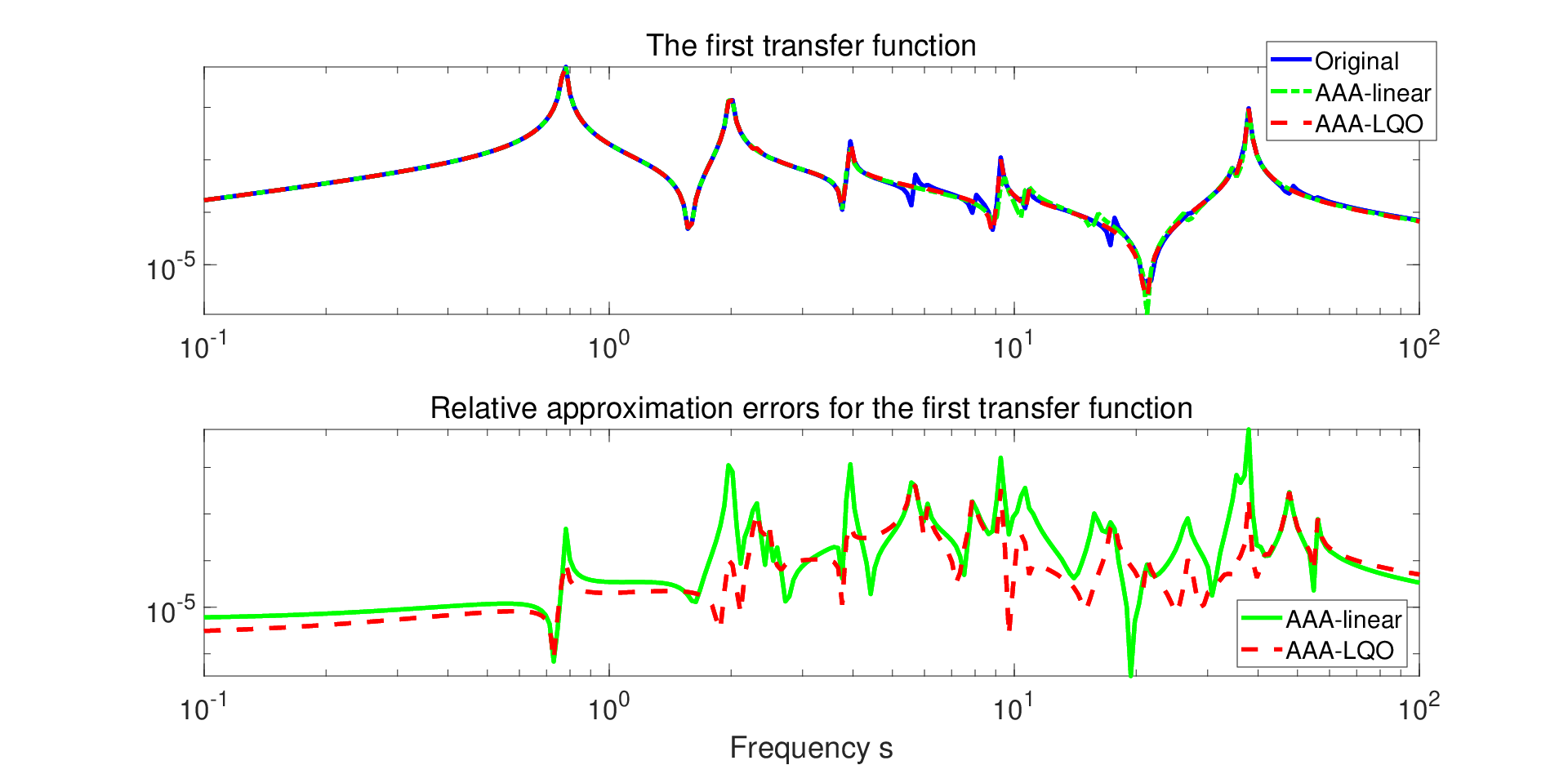
In the top plot of Figure 2, we show the magnitude of the first transfer function of the original system together with that of the linear AAA model and the first transfer function () of the AAA-LQO model. As expected, AAA model does a good job in matching the linear part of the output. Similarly, the AAA-LQO model also matches accurately. To better illustrate this, in the bottom plot of Figure 2, we depict the magnitude of the approximation errors in . The plot reveals that the AAA-LQO model has a smaller error for most of the frequency values, even in approximating . This happens despite the fact that it focuses on both and unlike the AAA model, which only tries to approximate .
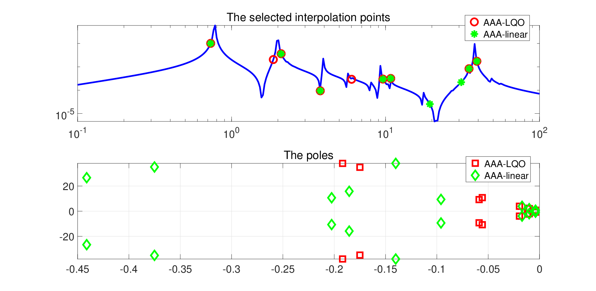
In Figure 3 we depict the selected support points (interpolation points) for both AAA and AAA-LQO algorithms (without the complex conjugate pairs), as well as the poles of the learned models (i.e., the eigenvalues of in both cases). Note that there are complex conjugate pairs of support points for each method. Even though some of the support points of AAA and AAA-LQO overlap, two of the pairs are different. This difference causes a big deviation in the the pole pattern as shown in the bottom plot, illustrating that even the linear part of the AAA-LQO approximant, i.e., , is fundamentally different than the linear AAA model. This is expected since AAA-LQO constructs and together by minimizing a joint LS measure in both and .
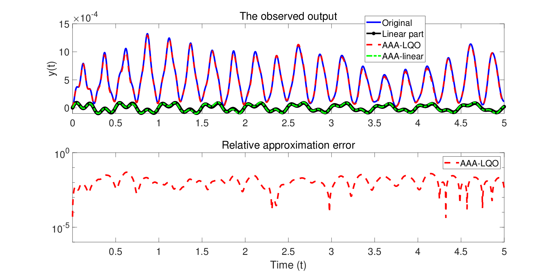
To show the overall performance of AAA-LQO in accurately approximating not only but also (the full LQO behavior), we perform a time-domain simulation of the original LQO system , the data-driven AAA-LQO model , and the linear AAA model by using as the control input. During the simulation of the original system , we also compute only the linear part of the output, which the AAA model should approximate well. The results are given in the top plot of Figure 4. The first observation is that the output of from AAA-LQO accurately replicates the output of . On the other hand, the linear AAA model completely misses the quadratic output and is only able to approximate the linear component in the output, as expected. The approximation error in the output corresponding to is depicted in the bottom plot of Figure 4.
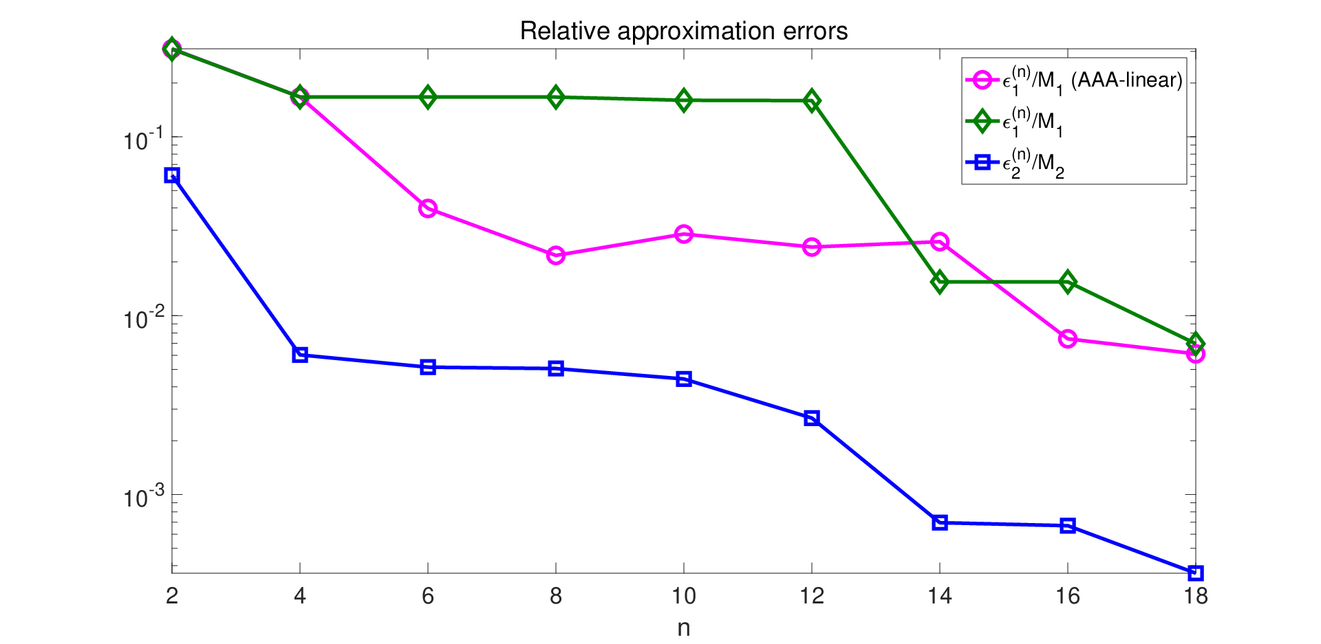
In Figure 5 we show the convergence behavior of AAA-LQO by plotting the evolution of the relative approximation errors ( and for all even values of . For a reference, we also depict the convergence behavior of AAA. The figure illustrates that after , both relative errors fall below the given tolerance of and the algorithm terminates.
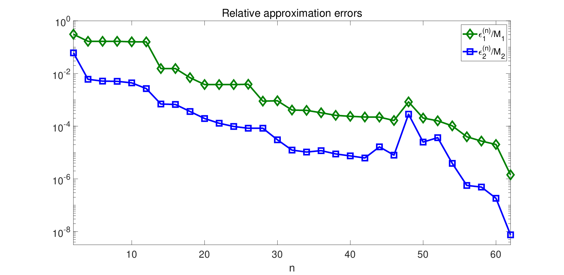
To investigate how the order of the AAA-LQO model varies based on the stopping tolerance, we set and run AAA-LQO for four tolerance values , , , and . The results are displayed in Table 1. For the case of , in Figure 6 we depict the convergence behavior of AAA-LQO by plotting and during the iteration.
6.2 Example 2
This model taken from [23] corresponds to an LQO system whose output measures a variance in the state-variable. A linear mass-spring-damper SISO dynamical system was modified in [22] by means of stochastic modeling, by replacing the physical parameters by independent random variables, yielding a linear dynamical system with multiple outputs. Based on this multiple output system, a SISO LQO system was derived in [23] where the output corresponds to the variance of tne original output (and thus is quadratic in nature). We refer the reader to [23] for further details. We obtain the measurements from a version of this model corresponding to an underlying LQO system of order .
The main difference from the previous example is that in this model the observed output does not have a linear component and depends on the state variable solely quadratically, i.e., in eq. 1. Hence, .
As sampling points , we choose logarithmically spaced points over the interval together with its conjugate pairs, leading to samples. Since , we only need to sample for . The corresponding data for the second transfer function are depicted in Figure 7.

We apply AAA-LQO with and (relative stopping criterion), obtaining a LQO model of order . To show the accuracy of the approximant, we perform time-domain simulations of the full model and the approximant with the input . We depict the observed outputs in the top plot of Figure 8, illustrating an accurate approximation. The corresponding output error is plotted in the bottom plot of Figure 8.

Finally, in Figure 9 we show the convergence behavior of AAA-LQO by plotting the evolution of relative approximation error .

Remark 5.
Since AAA-LQO uses a greedy selection scheme and is not a descent algorithm, there is no theoretical guarantee that the maximum approximation error will decrease monotonically. This can be seen in Figures 5, 6 and 9. This behavior was also observed in the original AAA algorithm; see, e.g, Application 6.3 in [20]. However, numerically the error indeed decreases monotonically with in most cases.
7 Conclusions
We have proposed a novel data-driven modeling method, called AAA-LQO, for linear systems with quadratic outputs (LQO). AAA-LQO extends the AAA algorithm to this new setting by first developing the barycentric representation theory for the two transfer functions arising in the analysis of LQO and then formulating a LS minimization framework to efficiently solve for the barycentric coefficients. The two numerical examples illustrate that AAA-LQO provides high-fidelity data-driven approximants to the original model.
The barycentric form we developed here for LQO systems offers promising research directions for modelling systems with general polynomial observation maps, as well as for nonlinearities appearing in the dynamical equation such as bilinear or quadratic-bilinear systems. These topics are the focus of on-going research.
8 Acknowledgements
The authors would like to thank Dr. Akil Narayan for providing the source codes for generating the numerical example presented in Section 6.2.
S. Gugercin was supported in parts by National Science Foundation under Grant No.
DMS-1720257 and DMS-1819110.
Part of this material is based upon work supported by the National Science
Foundation under Grant No. DMS-1439786 and by the Simons Foundation Grant No.
507536 while Gugercin was in residence at the
Institute for Computational and Experimental Research in Mathematics in
Providence, RI, during the “Model and dimension reduction in
uncertain and dynamic systems” program.
References
- [1] A. C. Antoulas. Approximation of large-scale dynamical systems. SIAM, Philadelphia, 2005.
- [2] A. C. Antoulas and B. D. 0. Anderson. On the scalar rational interpolation problem. IMA Journal of Mathematical Control and Information, 3(2-3):61–88, 1986.
- [3] A. C. Antoulas, C. Beattie, and S. Gugercin. Interpolatory methods for model reduction. Computational Science and Engineering 21. SIAM, Philadelphia, 2020.
- [4] A. C. Antoulas, A. C. Ionita, and S. Lefteriu. On two-variable rational interpolation. Linear Algebra and its Applications, 436(8):28890–2915, apr 2012.
- [5] A. C. Antoulas, S. Lefteriu, and A. C. Ionita. A tutorial introduction to the Loewner framework for model reduction. In Model Reduction and Approximation, chapter 8, pages 335–376. SIAM, 2017.
- [6] U. Baur, P. Benner, and L. Feng. Model order reduction for linear and nonlinear systems: A system-theoretic perspective. Archives of Computational Methods in Engineering, 21(4):331–358, 2014.
- [7] P. Benner, P. Goyal, and I. Pontes Duff. Gramians, energy functionals and balanced truncation for linear dynamical systems with quadratic outputs. Technical report, arXiv preprint available at https://arxiv.org/abs/1909.04597, 2019.
- [8] P. Benner, M. Ohlberger, A. Cohen, and K. Willcox. Model Reduction and Approximation. Society for Industrial and Applied Mathematics, Philadelphia, PA, 2017. doi:10.1137/1.9781611974829.
- [9] J.P. Berrut and L. N. Trefethen. Barycentric Lagrange interpolation. SIAM Rev., 46(3):501–517, aug 2004.
- [10] A. Carracedo Rodriguez and S. Gugercin. The p-AAA algorithm for data driven modeling of parametric dynamical systems. Technical report, arXiv preprint available at https://arxiv.org/abs/2003.06536, 2020.
- [11] Y. Chahlaoui and P. Van Dooren. A collection of benchmark examples for model reduction of linear time invariant dynamical systems. Technical Report 2002–2, SLICOT Working Note, 2002. Available from www.slicot.org.
- [12] F. Giri and E.-W. Bai, editors. Block-oriented Nonlinear System Identification. Lecture Notes in Control and Information Sciences. Springer-Verlag, London, 2010.
- [13] G. H. Golub and C. F. Van Loan. Matrix Computations. The Johns Hopkins University Press, fourth edition, 2013.
- [14] I. V. Gosea and A. C. Antoulas. A two-sided iterative framework for model reduction of linear systems with quadratic output. In Proceedings of the 58th Conference on Decision and Control (CDC), December 11-13, Nice, France, 2019.
- [15] I. V. Gosea and S. Güttel. Algorithms for the rational approximation of matrix-valued functions. Technical report, arXiv preprint available at https://arxiv.org/abs/2003.06410, 2020.
- [16] A. Juditsky, H. Hjalmarsson, A. Benveniste, B. Delyon, L. Ljung, J. Sjöberg, and Q. Zhang. Nonlinear black-box models in system identification: Mathematical foundations. Automatica, 31(12):1725 – 1750, 1995.
- [17] D. S. Karachalios, I. V. Gosea, and A. C. Antoulas. On bilinear time domain identification and reduction in the Loewner framework. In Model Reduction of Complex Dynamical Systems, International Series of Numerical Mathematics. Springer, 2020. accepted September 2020. URL: https://arxiv.org/abs/2003.08711.
- [18] D. S. Karachalios, I. V. Gosea, and A. C. Antoulas. The Loewner framework for nonlinear identification and reduction of Hammerstein cascaded dynamical systems. In Special Issue: 91st Annual Meeting of the International Association of Applied Mathematics and Mechanics (GAMM). Wiley, 2021.
- [19] P. Lietaert, J. Pérez, B. Vandereycken, and K. Meerbergen. Automatic rational approximation and linearization of nonlinear eigenvalue problems. Technical report, arXiv preprint available at https://arxiv.org/abs/1801.08622, 2018.
- [20] Y. Nakatsukasa, O. Sete, and L. N. Trefethen. The AAA algorithm for rational approximation. SIAM Journal on Scientific Computing, 40(3):A1494–A1522, 2018.
- [21] J. Nocedal and S. Wright. Numerical optimization. Springer Science & Business Media, 2006.
- [22] R. Pulch. Model order reduction and low-dimensional representations for random linear dynamical systems. Math. Comput. Simulat., 144:1–20, 2018.
- [23] R. Pulch and A. Narayan. Balanced truncation for model order reduction of linear dynamical systems with quadratic outputs. SIAM Journal on Scientific Computing, 41(4):A2270–A2295, 2019.
- [24] A. Quarteroni, A. Manzoni, and F. Negri. Reduced basis methods for partial differential equations: an introduction, volume 92. Springer, 2015.
- [25] W J. Rugh. Nonlinear System Theory - The Volterra/Wiener Approach. University Press, Baltimore, MD, 1981.
- [26] G. Scarciotti and A. Astolfi. Data-driven model reduction by moment matching for linear and nonlinear systems. Automatica, 79:340–351, 2017.
- [27] L.J. Tick. The estimation of ”transfer functions” of quadratic systems. Technometrics, 3(4):563–567, 1961.
- [28] R. Van Beeumen and K. Meerbergen. Model reduction by balanced truncation of linear systems with a quadratic output, pages 2033–2036. T.E. Simons, G. Psihoyios, Ch. Tsitouras (eds.), International Conference on Numerical Analysis and Applied Mathematics (ICNAAM). American Institute of Physics, 2010.
- [29] R. Van Beeumen, K. Van Nimmen, G. Lombaert, and K. Meerbergen. Model reduction for dynamical systems with quadratic output. Int. J. Numer. Meth. Engng., 91:229–248, 2012.
- [30] N. Wiener. Nonlinear problems in random theory. Wiley, New York, 1958.
Appendix A Proof of Lemma 2
Substitute and into (36) to obtain
and
where , and are as given in (34). Hence, write as
| (82) | ||||
Introduce the notation
| (83) |
Since holds, we can write
| (84) | ||||
By simplifying from both the numerator and the denominator in the above expression proves the first desired result in (39). The proof for follows similarly.