跳到论文正文
W Papers独立论文阅读器 arXiv:2102.13435 论文正文 计算阅读时间 · 0%
引用这篇论文根据当前论文元数据生成,正式投稿前建议核对。


License: arXiv.org perpetual non-exclusive license
arXiv:2102.13435v1 [stat.ME] 26 Feb 2021

Ensemble Conditional Variance Estimator for Sufficient Dimension ReductionThanks: efstathia.bura@tuwien.ac.at

Lukas Fertl Thanks: lukas.fertl@tuwien.ac.at Affiliation:   Institute of Statistics and Mathematical Methods in Economics Affiliation: Faculty of Mathematics and Geoinformation Affiliation: TU Wien, Vienna, Austria    Affiliation: Efstathia Bura Affiliation:   Institute of Statistics and Mathematical Methods in Economics Affiliation: Faculty of Mathematics and Geoinformation Affiliation: TU Wien, Vienna, Austria
Abstract

Ensemble Conditional Variance Estimation (ECVE) is a novel sufficient dimension reduction (SDR) method in regressions with continuous response and predictors. ECVE applies to general non-additive error regression models. It operates under the assumption that the predictors can be replaced by a lower dimensional projection without loss of information.It is a semiparametric forward regression model based exhaustive sufficient dimension reduction estimation method that is shown to be consistent under mild assumptions. It is shown to outperform central subspace mean average variance estimation (csMAVE), its main competitor, under several simulation settings and in a benchmark data set analysis.

1 Introduction

Let (Ω,ℱ,ℙ)(\Omega,{\mathcal{F}},\mathbb{P}) be a probability space. Let YY be a univariate continuous response and 𝐗{\mathbf{X}} a pp-variate continuous predictor, jointly distributed, with (Y,𝐗T)T:Ω→ℝp+1(Y,{\mathbf{X}}^{T})^{T}:\Omega\to{\mathbb{R}}^{p+1}. We consider the linear sufficient dimension reduction model

Y=gcs​(𝐁T​𝐗,ϵ),\displaystyle Y=g_{\textit{cs}}({\mathbf{B}}^{T}{\mathbf{X}},\epsilon), (1)

where 𝐗∈ℝp{\mathbf{X}}\in{\mathbb{R}}^{p} is independent of the random variable ϵ\epsilon, 𝐁{\mathbf{B}} is a p×kp\times k matrix of rank kk, and gcs:ℝk+1→ℝg_{\textit{cs}}:{\mathbb{R}}^{k+1}\to{\mathbb{R}} is an unknown non-constant function.

[ZZ10, Thm. 1] showed that if (Y,𝐗T)T(Y,{\mathbf{X}}^{T})^{T} has a joint continuous distribution, (1) is equivalent to

Y⟂⟂𝐗|𝐁T​𝐗,\displaystyle Y\perp\!\!\!\perp{\mathbf{X}}\mid{\mathbf{B}}^{T}{\mathbf{X}}, (2)

where the symbol ⟂⁣⟂\perp\!\!\!\perp indicates stochastic independence. The matrix 𝐁{\mathbf{B}} is not unique. It can be replaced by any basis of its column space, span⁡{𝐁}\operatorname{span}\{{\mathbf{B}}\}. Let 𝒮{\mathcal{S}} denote a subspace of ℝp{\mathbb{R}}^{p}, and let 𝐏𝒮\mathbf{P}_{{\mathcal{S}}} denote the orthogonal projection onto 𝒮{\mathcal{S}} with respect to the usual inner product. If the response YY and predictor vector 𝐗{\mathbf{X}} are independent conditionally on 𝐏𝒮​𝐗\mathbf{P}_{{\mathcal{S}}}{\mathbf{X}}, then 𝐏𝒮​𝐗\mathbf{P}_{{\mathcal{S}}}{\mathbf{X}} can replace 𝐗{\mathbf{X}} as the predictor in the regression of YY on 𝐗{\mathbf{X}} without loss of information. Such subspaces 𝒮{\mathcal{S}} are called dimension reduction subspaces and their intersection, provided it satisfies the conditional independence condition (2), is called the central subspace and denoted by 𝒮Y|𝐗\mathcal{S}_{Y\mid{\mathbf{X}}} [see [Coo98, p. 105], [Coo07]].

By their equivalence, under both models (1) and (2), FY|𝐗​(y)=FY|𝐁T​𝐗​(y)F_{Y\mid{\mathbf{X}}}(y)=F_{Y\mid{\mathbf{B}}^{T}{\mathbf{X}}}(y) and 𝒮Y|𝐗=span⁡{𝐁}\mathcal{S}_{Y\mid{\mathbf{X}}}=\operatorname{span}\{{\mathbf{B}}\}. Since the conditional distribution of Y|𝐗Y\mid{\mathbf{X}} is the same as that of Y|𝐁T​𝐗Y\mid{\mathbf{B}}^{T}{\mathbf{X}}, 𝐁T​𝐗{\mathbf{B}}^{T}{\mathbf{X}} contains all the information in 𝐗{\mathbf{X}} for modeling the target variable YY, and it can replace 𝐗{\mathbf{X}} without any loss of information.

If the error term in model (1) is additive with 𝔼⁡(ϵ∣𝐗)=0\mathbb{E}(\epsilon\mid{\mathbf{X}})=0, (1) reduces to Y=g⁡(𝐁T​𝐗)+ϵY=g({\mathbf{B}}^{T}{\mathbf{X}})+\epsilon. Now, 𝔼⁡(Y∣𝐗)=𝔼⁡(Y∣𝐁T​𝐗)=𝔼⁡(Y∣𝐏𝒮​𝐗)\mathbb{E}(Y\mid{\mathbf{X}})=\mathbb{E}(Y\mid{\mathbf{B}}^{T}{\mathbf{X}})=\mathbb{E}(Y\mid\mathbf{P}_{{\mathcal{S}}}{\mathbf{X}}), where 𝒮=span⁡{𝐁}{\mathcal{S}}=\operatorname{span}\{{\mathbf{B}}\}. The mean subspace, denoted by 𝒮𝔼⁡(Y∣𝐗)\mathcal{S}_{\mathbb{E}\left(Y\mid{\mathbf{X}}\right)}, is the intersection of all subspaces 𝒮{\mathcal{S}} such that 𝔼⁡(Y∣𝐗)=𝔼⁡(Y∣𝐏𝒮​𝐗)\mathbb{E}(Y\mid{\mathbf{X}})=\mathbb{E}(Y\mid\mathbf{P}_{{\mathcal{S}}}{\mathbf{X}}) [CL02]. In this case, (1) becomes the classic mean subspace model with span⁡{𝐁}=𝒮𝔼⁡(Y∣𝐗)\operatorname{span}\{{\mathbf{B}}\}=\mathcal{S}_{\mathbb{E}\left(Y\mid{\mathbf{X}}\right)}. [CL02] showed that the mean subspace is a subset of the central subspace, 𝒮𝔼⁡(Y∣𝐗)⊆𝒮Y|𝐗\mathcal{S}_{\mathbb{E}\left(Y\mid{\mathbf{X}}\right)}\subseteq\mathcal{S}_{Y\mid{\mathbf{X}}}.

Several linear sufficient dimension reduction (SDR) methods estimate 𝒮𝔼⁡(Y∣𝐗)\mathcal{S}_{\mathbb{E}\left(Y\mid{\mathbf{X}}\right)} consistently ([AC09, MZ13, Li18, XTLZ02]). Linear refers to the reduction being a linear transformation of the predictor vector. Minimum Average Variance Estimation (MAVE) [XTLZ02] is the most competitive and accurate method among them. MAVE differentiates from the majority of SDR methods, in that it is not inverse regression based such as, for example, the widely used Sliced Inverse Regression (SIR, [Li91]). MAVE requires minimal assumptions on the distribution of (Y,𝐗T)T(Y,{\mathbf{X}}^{T})^{T} and is based on estimating the gradients of the regression function E⁡(Y∣𝐗)E(Y\mid{\mathbf{X}}) via local-linear smoothing [CD88].

The central subspace mean average variance estimation (csMAVE) [WX08, WY19] is the extension of MAVE that consistently and exhaustively estimates the span⁡{𝐁}\operatorname{span}\{{\mathbf{B}}\} in model (1) without restrictive assumptions limiting its applicability. csMAVE has remained the gold standard since it was proposed by [WX08]. It is based on repeatedly applying MAVE on the sliced target variables fu(Y)=𝟏{su−1<Y≤su}f_{u}(Y)=\mathbf{1}_{\{s_{u-1}<Y\leq s_{u}\}} for s1<…<sHs_{1}<\ldots<s_{H}. [WX08] showed that the mean subspaces of the sliced YY can be combined to recover the central subspace 𝒮Y|𝐗\mathcal{S}_{Y\mid{\mathbf{X}}}.

Several papers made contributions in establishing a road path from the central mean to the central subspace [see [YL11] for a list of references]. [YL11] recognized that these approaches pointed to the same direction: if one can estimate the central mean subspace of 𝔼⁡(f⁡(𝐗)∣Y)\mathbb{E}(f({\mathbf{X}})\mid Y) for sufficiently many functions f∈ℱf\in\mathcal{F} for a family of functions ℱ\mathcal{F}, then one can recover the central subspace. Such families that are rich enough to obtain the desired outcome are called characterizing ensembles by [YL11], who also proposed and studied such functional families [see also [Li18] for an overview].

In this paper, we extend the conditional variance estimator (CVE) [FB21] to the exhaustive ensemble conditional variance estimator for recovering fully the central subspace 𝒮Y|𝐗\mathcal{S}_{Y\mid{\mathbf{X}}}. Conditional variance estimation is a semi-parametric method for the estimation of 𝒮𝔼⁡(Y∣𝐗)\mathcal{S}_{\mathbb{E}\left(Y\mid{\mathbf{X}}\right)} consistently under minimal regularity assumptions on the distribution of (Y,𝐗T)T(Y,{\mathbf{X}}^{T})^{T}. In contrast to other SDR approaches, it operates by identifying the orthogonal complement of 𝒮𝔼⁡(Y∣𝐗)\mathcal{S}_{\mathbb{E}\left(Y\mid{\mathbf{X}}\right)}. In this paper we apply the conditional variance estimator (CVE) to identify the mean subspace 𝒮𝔼​(ft​(Y)∣𝐗)\mathcal{S}_{\mathbb{E}\left(f_{t}(Y)\mid{\mathbf{X}}\right)} of transformed responses ft​(Y)f_{t}(Y), where ftf_{t} are elements of an ensemble ℱ={ft:t∈ΩT}\mathcal{F}=\{f_{t}:t\in\Omega_{T}\}, and then combine them to form the central subspace 𝒮Y|𝐗\mathcal{S}_{Y\mid{\mathbf{X}}}.

The paper is organized as follows. In Section 2 we define the notation and concepts we use throughout the paper. A short overview of ensembles is given in Section 2.1. The ensemble conditional variance estimator (ECVE) is introduced in Section 3 and the estimation procedure in Section 4. In Section 5, the consistency of the ensemble conditional variance estimator for the central subspace is shown. We assess and compare the performance of the estimator vis-a-vis csMAVE via simulations in Section 6 and by applying it to the Boston Housing data in Section 7. We conclude in Section 8.

2 Preliminaries

We denote by F𝐙F_{\mathbf{Z}} the cumulative distribution function (cdf) of a random variable or vector 𝐙{\mathbf{Z}}. We drop the subscript, when the attribution is clear from the context. For a matrix 𝐀{\mathbf{A}}, ‖𝐀‖\|{\mathbf{A}}\| denotes its Frobenius norm, and ‖𝒂‖\|\bm{a}\| the Euclidean norm for a vector 𝒂\bm{a}. Scalar product refers to the usual Euclidean scalar product, and ⟂\perp denotes orthogonality with respect to it. The probability density function of 𝐗{\mathbf{X}} is denoted by f𝐗f_{{\mathbf{X}}}, and its support by supp​(f𝐗)\mbox{supp}(f_{{\mathbf{X}}}). The notation Y⟂⟂𝐗Y\perp\!\!\!\perp{\mathbf{X}} signifies stochastic independence of the random vector 𝐗{\mathbf{X}} and random variable YY. The jj-th standard basis vector with zeroes everywhere except for 1 on the jj-th position is denoted by 𝐞j∈ℝp\mathbf{e}_{j}\in{\mathbb{R}}^{p}, 𝜾p=(1,1,…,1)T∈ℝp\mbox{\boldmath$\iota$}_{p}=(1,1,\ldots,1)^{T}\in{\mathbb{R}}^{p}, and 𝐈p=(𝐞1,…,𝐞p){\mathbf{I}}_{p}=(\mathbf{e}_{1},\ldots,\mathbf{e}_{p}) is the identity matrix of order pp. For any matrix 𝐌∈ℝp×q{\mathbf{M}}\in{\mathbb{R}}^{p\times q}, 𝐏𝐌\mathbf{P}_{{\mathbf{M}}} denotes the orthogonal projection matrix on its column or range space span⁡{𝐌}\operatorname{span}\{{\mathbf{M}}\}; i.e., 𝐏𝐌=𝐏span⁡{𝐌}=𝐌​(𝐌T​𝐌)−1​𝐌T∈ℝp×p\mathbf{P}_{{\mathbf{M}}}=\mathbf{P}_{\operatorname{span}\{{\mathbf{M}}\}}={\mathbf{M}}({\mathbf{M}}^{T}{\mathbf{M}})^{-1}{\mathbf{M}}^{T}\in{\mathbb{R}}^{p\times p}.

For q≤pq\leq p,

𝒮⁡(p,q)={𝐕∈ℝp×q:𝐕T​𝐕=𝐈q},{\mathcal{S}}(p,q)=\{{\mathbf{V}}\in{\mathbb{R}}^{p\times q}:{\mathbf{V}}^{T}{\mathbf{V}}={\mathbf{I}}_{q}\}, (3)

denotes the Stiefel manifold that comprizes of all p×qp\times q matrices with orthonormal columns. 𝒮⁡(p,q){\mathcal{S}}(p,q) is compact with dim(𝒮⁡(p,q))=p​q−q⁡(q+1)/2\dim({\mathcal{S}}(p,q))=pq-q(q+1)/2 [see [Boo02] and Section 2.1 of [Tag11]]. The set

G​r​(p,q)=𝒮⁡(p,q)/𝒮⁡(q,q)Gr(p,q)={\mathcal{S}}(p,q)/{\mathcal{S}}(q,q) (4)

denotes a Grassmann manifold [GH94] that contains all qq-dimensional subspaces in ℝp{\mathbb{R}}^{p}. G​r​(p,q)Gr(p,q) is the quotient space of 𝒮⁡(p,q){\mathcal{S}}(p,q) with all q×qq\times q orthonormal matrices in 𝒮⁡(q,q){\mathcal{S}}(q,q).

2.1 Ensembles

[YL11] introduced ensembles as a device to extend mean subspace to central subspace SDR methods. The ensemble approach of combining mean subspaces to span the central subspace comprizes of two components: (a) a rich family of functions of transformations for the response and (b) a sampling mechanism for drawing the functions from the ensemble to ascertain coverage of the central subspace. To distinguish between families of functions and ensembles, [YL11] use the term parametric ensemble, which we define next.

Definition.

A family ℱ\mathcal{F} of measurable functions from ℝ{\mathbb{R}} to ℝ{\mathbb{R}} is called an ensemble. If ℱ\mathcal{F} is a family of measurable functions with respect to an index set ΩT\Omega_{T}; i.e. ℱ={ft:t∈ΩT}\mathcal{F}=\{f_{t}:t\in\Omega_{T}\}, ℱ\mathcal{F} is called a parametric ensemble.

Let ℱ\mathcal{F} be an ensemble, f∈ℱf\in\mathcal{F} and let f⁡(Y)f(Y), for YY following model (1). The space 𝒮𝔼⁡(f⁡(Y)∣𝐗){\mathcal{S}}_{\mathbb{E}(f(Y)\mid{\mathbf{X}})} is defined to be the mean subspace of the transformed random variable f⁡(Y)f(Y) [see [Coo98] or [CL02]].

Definition.

An ensemble ℱ\mathcal{F} characterizes the central subspace 𝒮Y|𝐗\mathcal{S}_{Y\mid{\mathbf{X}}}, if

span⁡{𝒮𝔼​(ft​(Y)∣𝐗):ft∈ℱ}=𝒮Y|𝐗\displaystyle\operatorname{span}\{\mathcal{S}_{\mathbb{E}\left(f_{t}(Y)\mid{\mathbf{X}}\right)}:f_{t}\in\mathcal{F}\}=\mathcal{S}_{Y\mid{\mathbf{X}}} (5)

As an example, the parametric ensemble ℱ={ft:t∈ΩT}={1{z≤t}:t∈ℝ}\mathcal{F}=\{f_{t}:t\in\Omega_{T}\}=\{1_{\{z\leq t\}}:t\in{\mathbb{R}}\} can characterize the central subspace 𝒮Y|𝐗\mathcal{S}_{Y\mid{\mathbf{X}}}. That is, 𝔼​(ft​(Y)|𝐗)\mathbb{E}(f_{t}(Y)|{\mathbf{X}}) is the conditional cumulative distribution function evaluated at tt. To see this, let 𝐁∈𝒮⁡(p,k){\mathbf{B}}\in{\mathcal{S}}(p,k) be such that 𝔼⁡(ft​(Y)∣𝐗)=𝔼⁡(ft​(Y)∣𝐁T​𝐗)\mathbb{E}(f_{t}(Y)\mid{\mathbf{X}})=\mathbb{E}(f_{t}(Y)\mid{\mathbf{B}}^{T}{\mathbf{X}}) for all tt. Then, FY|𝐗​(t)=𝔼⁡(ft​(Y)∣𝐗)=𝔼⁡(ft​(Y)∣𝐁T​𝐗)=FY|𝐁T​𝐗​(t)F_{Y\mid{\mathbf{X}}}(t)=\mathbb{E}(f_{t}(Y)\mid{\mathbf{X}})=\mathbb{E}(f_{t}(Y)\mid{\mathbf{B}}^{T}{\mathbf{X}})=F_{Y\mid{\mathbf{B}}^{T}{\mathbf{X}}}(t) for all tt. Varying over the parametric ensemble ℱ\mathcal{F}, in this case over t∈ℝt\in{\mathbb{R}}, obtains the conditional cumulative distribution function. This indicator ensemble fully recovers the conditional distribution of Y|𝐗Y\mid{\mathbf{X}} and, thus, also the central subspace 𝒮Y|𝐗\mathcal{S}_{Y\mid{\mathbf{X}}},

span{𝒮𝔼​(ft​(Y)∣𝐗):ft∈ℱ}=span{𝒮𝔼(1{Y≤t}∣𝐗):t∈ℝ}=𝒮Y|𝐗\displaystyle\operatorname{span}\{\mathcal{S}_{\mathbb{E}\left(f_{t}(Y)\mid{\mathbf{X}}\right)}:f_{t}\in\mathcal{F}\}=\operatorname{span}\{\mathcal{S}_{\mathbb{E}\left(1_{\{Y\leq t\}}\mid{\mathbf{X}}\right)}:t\in{\mathbb{R}}\}=\mathcal{S}_{Y\mid{\mathbf{X}}}

We reproduce a list of parametric ensembles ℱ\mathcal{F}, and associated regularity conditions, that can characterize 𝒮Y|𝐗\mathcal{S}_{Y\mid{\mathbf{X}}} from [YL11] next.

Characteristic ensemble

ℱ={ft:t∈ΩT}={exp(it⋅):t∈ℝ}\mathcal{F}=\{f_{t}:t\in\Omega_{T}\}=\{\exp(it\cdot):t\in{\mathbb{R}}\}

Indicator ensemble

ℱ={1{z≤t}:t∈ℝ}\mathcal{F}=\{1_{\{z\leq t\}}:t\in{\mathbb{R}}\}, where span⁡{𝒮𝔼​(ft​(Y)∣𝐗):ft∈ℱ}\operatorname{span}\{\mathcal{S}_{\mathbb{E}\left(f_{t}(Y)\mid{\mathbf{X}}\right)}:f_{t}\in\mathcal{F}\} recovers the conditional cumulative distribution function

Kernel ensemble

ℱ={h−1K((z−t)/h):t∈ℝ,h>0}\mathcal{F}=\{h^{-1}K\left((z-t)/h\right):t\in{\mathbb{R}},h>0\}, where KK is a kernel suitable for density estimation, and span⁡{𝒮𝔼​(ft​(Y)∣𝐗):ft∈ℱ}\operatorname{span}\{\mathcal{S}_{\mathbb{E}\left(f_{t}(Y)\mid{\mathbf{X}}\right)}:f_{t}\in\mathcal{F}\} recovers the conditional density

Polynomial ensemble

ℱ={zt:t=1,2,3,…}\mathcal{F}=\{z^{t}:t=1,2,3,...\}, where span⁡{𝒮𝔼​(ft​(Y)∣𝐗):ft∈ℱ}\operatorname{span}\{\mathcal{S}_{\mathbb{E}\left(f_{t}(Y)\mid{\mathbf{X}}\right)}:f_{t}\in\mathcal{F}\} recovers the conditional moment generating function

Box-Cox ensemble

ℱ={(zt−1)/t:t≠0}∪{log⁡(z):t=0}\mathcal{F}=\{(z^{t}-1)/t:t\neq 0\}\cup\{\log(z):t=0\} Box-Cox Transforms

Wavelet ensemble

Haar Wavelets

The characteristic and indicator ensembles describe the conditional characteristic and distribution function of Y|𝐗Y\mid{\mathbf{X}}, respectively, which always exist and determine the distribution uniquely. If the conditional density function fY|𝐗f_{Y\mid{\mathbf{X}}} of Y|𝐗Y\mid{\mathbf{X}} exists, then the kernel ensemble characterizes the conditional distribution Y|𝐗Y\mid{\mathbf{X}}. Further, if the conditional moment generating function exists, then the polynomial ensemble characterizes 𝒮Y|𝐗\mathcal{S}_{Y\mid{\mathbf{X}}}. [YL11] used the ensemble device to extend MAVE [XTLZ02], which targets the mean subspace, to its ensemble version that also estimates the central subspace 𝒮Y|𝐗\mathcal{S}_{Y\mid{\mathbf{X}}} consistently.

Theorem 1 [YL11, Thm 2.1] establishes when an ensemble ℱ\mathcal{F} is rich enough to characterize 𝒮Y|𝐗\mathcal{S}_{Y\mid{\mathbf{X}}}.

Theorem 1.

Let ℬ={1A:A​ is a Borel set in​supp​(Y)}\mathcal{B}=\{1_{A}:A\text{ is a Borel set in}\;\text{supp}(Y)\} be the set of indicator functions on supp​(Y)\text{supp}(Y) and L2​(FY)L^{2}(F_{Y}) be the set of square integrable random variables with respect to the distribution FYF_{Y} of the response YY. If ℱ⊆L2​(FY)\mathcal{F}\subseteq L^{2}(F_{Y}) is dense in ℬ⊆L2​(FY)\mathcal{B}\subseteq L^{2}(F_{Y}), then the ensemble ℱ\mathcal{F} characterizes the central subspace 𝒮Y|𝐗\mathcal{S}_{Y\mid{\mathbf{X}}}.

In Theorem 2 we show that finitely many functions of an ensemble ℱ\mathcal{F} are sufficient to characterize the central subspace 𝒮Y|𝐗\mathcal{S}_{Y\mid{\mathbf{X}}}.

Theorem 2.

If a parametric ensemble ℱ\mathcal{F} characterizes 𝒮Y|𝐗\mathcal{S}_{Y\mid{\mathbf{X}}}, then there exist finitely many functions ft∈ℱf_{t}\in\mathcal{F}, with t=1,…,mt=1,\ldots,m and m∈ℕm\in\mathbb{N}, such that

span{𝒮𝔼​(ft​(Y)∣𝐗):t∈1,…,m}=𝒮Y|𝐗\displaystyle\operatorname{span}\{\mathcal{S}_{\mathbb{E}\left(f_{t}(Y)\mid{\mathbf{X}}\right)}:t\in 1,\ldots,m\}=\mathcal{S}_{Y\mid{\mathbf{X}}}
Proof:

Let k=dim(𝒮Y|𝐗)≤pk=\dim(\mathcal{S}_{Y\mid{\mathbf{X}}})\leq p. Since ℱ\mathcal{F} characterizes 𝒮Y|𝐗\mathcal{S}_{Y\mid{\mathbf{X}}}, dim(𝒮𝔼​(ft​(Y)∣𝐗))=kt≤k\dim(\mathcal{S}_{\mathbb{E}\left(f_{t}(Y)\mid{\mathbf{X}}\right)})=k_{t}\leq k by (5) for any tt. If kt=0k_{t}=0, 𝒮𝔼​(ft​(Y)∣𝐗)={𝟎}\mathcal{S}_{\mathbb{E}\left(f_{t}(Y)\mid{\mathbf{X}}\right)}=\{{\mathbf{0}}\} so the corresponding ftf_{t} does not contribute to (5). Assume kt≥1k_{t}\geq 1. If there were infinitely many 𝒮𝔼​(ft​(Y)∣𝐗)≠{𝟎}\mathcal{S}_{\mathbb{E}\left(f_{t}(Y)\mid{\mathbf{X}}\right)}\neq\{{\mathbf{0}}\} of dimension at least 1, whose span is 𝒮Y|𝐗\mathcal{S}_{Y\mid{\mathbf{X}}}, then infinitely as many are identical, otherwise the dimension of the central subspace 𝒮Y|𝐗\mathcal{S}_{Y\mid{\mathbf{X}}} would be infinite, contradicting that dim(𝒮Y|𝐗)=k<∞\dim(\mathcal{S}_{Y\mid{\mathbf{X}}})=k<\infty. ∎

The importance of Theorem 2 lies in the fact that the search to characterize the central subspace is over a finite set, even though it does not offer tools for identifying the elements of the ensemble.

3 Ensemble CVE

Throughout the paper, we refer to the following assumptions as needed.

(E.1).

Model (1), Y=gcs​(𝐁T​𝐗,ϵ)Y=g_{\textit{cs}}({\mathbf{B}}^{T}{\mathbf{X}},\epsilon) holds with Y∈ℝY\in{\mathbb{R}}, gcs:ℝk×ℝ→ℝg_{\textit{cs}}:{\mathbb{R}}^{k}\times{\mathbb{R}}\to{\mathbb{R}} non constant in the first argument, 𝐁=(𝐛1,…,𝐛k)∈𝒮⁡(p,k){\mathbf{B}}=({\mathbf{b}}_{1},...,{\mathbf{b}}_{k})\in{\mathcal{S}}(p,k), 𝐗∈ℝp{\mathbf{X}}\in{\mathbb{R}}^{p} is independent of ϵ\epsilon, the distribution of 𝐗{\mathbf{X}} is absolutely continuous with respect to the Lebesgue measure in ℝp{\mathbb{R}}^{p}, supp​(f𝐗)\text{supp}(f_{\mathbf{X}}) is convex, and 𝕍​ar​(𝐗)=𝚺𝐱\mathbb{V}\mathrm{ar}({\mathbf{X}})=\mbox{\boldmath$\Sigma$}_{{\mathbf{x}}} is positive definite.

(E.2).

The density f𝐗:ℝp→[0,∞)f_{\mathbf{X}}:{\mathbb{R}}^{p}\to[0,\infty) of 𝐗{\mathbf{X}} is twice continuously differentiable with compact support supp​(f𝐗)\text{supp}(f_{\mathbf{X}}).

(E.3).

For a parametric ensemble ℱ\mathcal{F}, its index set ΩT\Omega_{T} is endowed with a probability measure FTF_{T} such that for all t∈ΩTt\in\Omega_{T} with 𝒮𝔼​(ft​(Y)∣𝐗)≠{𝟎}\mathcal{S}_{\mathbb{E}\left(f_{t}(Y)\mid{\mathbf{X}}\right)}\neq\{{\mathbf{0}}\},

ℙFT​({t~∈ΩT:𝒮𝔼​(ft~​(Y)∣𝐗)=𝒮𝔼​(ft​(Y)∣𝐗)})>0\displaystyle\mathbb{P}_{F_{T}}\left(\{\tilde{t}\in\Omega_{T}:{\mathcal{S}}_{\mathbb{E}(f_{\tilde{t}}(Y)\mid{\mathbf{X}})}=\mathcal{S}_{\mathbb{E}\left(f_{t}(Y)\mid{\mathbf{X}}\right)}\}\right)>0
(E.4).

For an ensemble ℱ\mathcal{F} we assume that for all f∈ℱf\in\mathcal{F}, the conditional expectation

𝔼⁡(f⁡(Y)∣𝐗)\displaystyle\mathbb{E}\left(f(Y)\mid{\mathbf{X}}\right)

is twice continuously differentiable in the conditioning argument. Further, for all f∈ℱf\in\mathcal{F}

𝔼⁡(|f⁡(Y)|8)<∞\displaystyle\mathbb{E}(|f(Y)|^{8})<\infty

Assumption (E.1) assures the existence and uniqueness of 𝒮Y|𝐗=span⁡{𝐁}\mathcal{S}_{Y\mid{\mathbf{X}}}=\operatorname{span}\{{\mathbf{B}}\}. Furthermore, it allows the mean subspace to be a proper subset of the central subspace, i.e. 𝒮𝔼⁡(Y∣𝐗)⊊𝒮Y|𝐗\mathcal{S}_{\mathbb{E}\left(Y\mid{\mathbf{X}}\right)}\subsetneq\mathcal{S}_{Y\mid{\mathbf{X}}}. In Assumption (E.2), the compactness assumption for supp​(f𝐗)\text{supp}(f_{\mathbf{X}}) is not as restrictive as it might seem. [YLC08, Prop. 11] showed that there is a compact set K⊂ℝpK\subset{\mathbb{R}}^{p} such that 𝒮Y∣𝐗|K=𝒮Y|𝐗\mathcal{S}_{Y\mid{\mathbf{X}}_{|K}}=\mathcal{S}_{Y\mid{\mathbf{X}}}, where 𝐗|K=𝐗1{𝐗∈K}{\mathbf{X}}_{|K}={\mathbf{X}}1_{\{{\mathbf{X}}\in K\}}. Assumption (E.3) simply states that the set of indices that characterize the central subspace 𝒮Y|𝐗\mathcal{S}_{Y\mid{\mathbf{X}}} is not a null set. In practice, the choice of the probability measure FTF_{T} on the index set ΩT\Omega_{T} of a parametric ensemble ℱ\mathcal{F} can always guarantee the fulfillment of this assumption. If the characteristic or indicator ensemble are used, (E.4) states that the conditional characteristic or distribution function are twice continuously differentiable. In this case, the 8t​hth moments exist since the complex exponential and indicator functions are bounded.

Definition.

For q≤p∈ℕq\leq p\in\mathbb{N}, f∈ℱf\in\mathcal{F}, and any 𝐕∈S⁡(p,q){\mathbf{V}}\in S(p,q), we define

L~ℱ​(𝐕,𝐬0,f)=𝕍​ar​(f⁡(Y)∣𝐗∈𝐬0+span⁡{𝐕})\tilde{L}_{\mathcal{F}}({\mathbf{V}},\mathbf{s}_{0},f)=\mathbb{V}\mathrm{ar}\left(f(Y)\mid{\mathbf{X}}\in\mathbf{s}_{0}+\operatorname{span}\{{\mathbf{V}}\}\right) (6)

where 𝐬0∈ℝp\mathbf{s}_{0}\in{\mathbb{R}}^{p} is a non-random shifting point.

Definition.

Let ℱ\mathcal{F} be a parametric ensemble and FTF_{T} a cumulative distribution function (cdf) on the index set ΩT\Omega_{T}. For q≤pq\leq p, and any 𝐕∈S⁡(p,q){\mathbf{V}}\in S(p,q), we define

Lℱ​(𝐕)\displaystyle L_{\mathcal{F}}({\mathbf{V}}) =∫ΩT∫ℝpL~​(𝐕,𝐱,ft)​d​F𝐗​(𝐱)​d​FT​(t)\displaystyle=\int_{\Omega_{T}}\int_{{\mathbb{R}}^{p}}\tilde{L}({\mathbf{V}},{\mathbf{x}},f_{t})dF_{{\mathbf{X}}}({\mathbf{x}})dF_{T}(t) (7)
=𝔼t∼FT​(𝔼𝐗​(L~ℱ​(𝐕,𝐗,ft)))=𝔼t∼FT​(Lℱ∗​(𝐕,ft)),\displaystyle=\mathbb{E}_{t\sim F_{T}}\left(\mathbb{E}_{\mathbf{X}}\left(\tilde{L}_{\mathcal{F}}({\mathbf{V}},{\mathbf{X}},f_{t})\right)\right)=\mathbb{E}_{t\sim F_{T}}(L_{\mathcal{F}}^{*}({\mathbf{V}},f_{t})),

where F𝐗F_{{\mathbf{X}}} is the cdf of 𝐗{\mathbf{X}},and

Lℱ∗​(𝐕,ft)=𝔼𝐗​(L~ℱ​(𝐕,𝐗,ft)).\displaystyle L_{\mathcal{F}}^{*}({\mathbf{V}},f_{t})=\mathbb{E}_{\mathbf{X}}\left(\tilde{L}_{\mathcal{F}}({\mathbf{V}},{\mathbf{X}},f_{t})\right). (8)

For the identity function, ft0​(z)=zf_{t_{0}}(z)=z, (8) is the target function of the conditional variance estimation proposed in [FB21]. If the random variable tt is concentrated on t0t_{0}; i.e., t∼δt0t\sim\delta_{t_{0}}, then the ensemble conditional variance estimator (ECVE) coincides with the conditional variance estimator (CVE).

The following theorem will be used in establishing the main result of this paper, which obtains the exhaustive sufficient reduction of the conditional distribution of YY given the predictor vector 𝐗{\mathbf{X}}.

Theorem 3.

Assume (E.1) and (E.2) hold, in particular model (1) holds. Let 𝐁~\widetilde{{\mathbf{B}}} be a basis of 𝒮𝔼​(ft​(Y)∣𝐗)\mathcal{S}_{\mathbb{E}\left(f_{t}(Y)\mid{\mathbf{X}}\right)}; i.e. span⁡{𝐁~}=𝒮𝔼​(ft​(Y)∣𝐗)⊆𝒮Y|𝐗=span⁡{𝐁}\operatorname{span}\{\widetilde{{\mathbf{B}}}\}=\mathcal{S}_{\mathbb{E}\left(f_{t}(Y)\mid{\mathbf{X}}\right)}\subseteq\mathcal{S}_{Y\mid{\mathbf{X}}}=\operatorname{span}\{{\mathbf{B}}\}. Then, for any f∈ℱf\in\mathcal{F} for which assumption (E.4) holds,

f⁡(Y)=g⁡(𝐁~T​𝐗)+ϵ~,\displaystyle f(Y)=g(\widetilde{{\mathbf{B}}}^{T}{\mathbf{X}})+\tilde{\epsilon}, (9)

with 𝔼⁡(ϵ~∣𝐗)=0\mathbb{E}(\tilde{\epsilon}\mid{\mathbf{X}})=0 and g:ℝkt→ℝg:{\mathbb{R}}^{k_{t}}\to{\mathbb{R}} is a twice continuously differentiable function, where kt=dim(𝒮𝔼​(ft​(Y)∣𝐗))k_{t}=\dim(\mathcal{S}_{\mathbb{E}\left(f_{t}(Y)\mid{\mathbf{X}}\right)}).

By Theorem 3, any response YY can be written as an additive error via the decomposition (9). The predictors and the additive error term are only required to be conditionally uncorrelated in model (9). The conditional variance estimator [FB21] also estimated 𝐁~\widetilde{{\mathbf{B}}} in (9) but under the more restrictive condition of predictor and error independence.

Proof of Theorem 3.
f⁡(Y)\displaystyle f(Y) =𝔼⁡(f⁡(Y)∣𝐗)+f⁡(Y)−𝔼⁡(f⁡(Y)∣𝐗)⏟ϵ~=𝔼⁡(f⁡(Y)∣𝐗)+ϵ~\displaystyle=\mathbb{E}\left(f(Y)\mid{\mathbf{X}}\right)+\underbrace{f(Y)-\mathbb{E}\left(f(Y)\mid{\mathbf{X}}\right)}_{\tilde{\epsilon}}=\mathbb{E}\left(f(Y)\mid{\mathbf{X}}\right)+\tilde{\epsilon}
=𝔼⁡(f⁡(Y)|𝐁~T​𝐗)+ϵ~=g⁡(𝐁~T​𝐗)+ϵ~\displaystyle=\mathbb{E}\left(f(Y)|\widetilde{{\mathbf{B}}}^{T}{\mathbf{X}}\right)+\tilde{\epsilon}=g(\widetilde{{\mathbf{B}}}^{T}{\mathbf{X}})+\tilde{\epsilon}

where g⁡(𝐁~T​𝐗)=𝔼⁡(f⁡(Y)|𝐁~T​𝐗)g(\widetilde{{\mathbf{B}}}^{T}{\mathbf{X}})=\mathbb{E}\left(f(Y)|\widetilde{{\mathbf{B}}}^{T}{\mathbf{X}}\right). By the tower property of the conditional expectation, 𝔼⁡(ϵ~∣𝐗)=𝔼⁡(f⁡(Y)∣𝐗)−𝔼⁡(𝔼⁡(f⁡(Y)∣𝐗)∣𝐗)=𝔼⁡(f⁡(Y)∣𝐗)−𝔼⁡(f⁡(Y)∣𝐗)=𝟎\mathbb{E}(\tilde{\epsilon}\mid{\mathbf{X}})=\mathbb{E}(f(Y)\mid{\mathbf{X}})-\mathbb{E}(\mathbb{E}(f(Y)\mid{\mathbf{X}})\mid{\mathbf{X}})=\mathbb{E}(f(Y)\mid{\mathbf{X}})-\mathbb{E}(f(Y)\mid{\mathbf{X}})={\mathbf{0}}. The function gg is twice continuous differentiable by (E.4). ∎

Theorem 4.

Assume (E.1) and (E.2) hold. Let ℱ\mathcal{F} be a parametric ensemble, 𝐬0∈supp​(f𝐗)⊂ℝp\mathbf{s}_{0}\in\text{supp}(f_{\mathbf{X}})\subset{\mathbb{R}}^{p}, 𝐕∈S⁡(p,q){\mathbf{V}}\in S(p,q) defined in (3). Then, for any f∈ℱf\in\mathcal{F} for which assumption (E.4) holds,

L~ℱ​(𝐕,𝐬0,f)=μ2​(𝐕,𝐬0,f)−μ12​(𝐕,𝐬0,f)+𝕍​ar​(ϵ~∣𝐗∈𝐬0+span⁡{𝐕})\displaystyle\tilde{L}_{\mathcal{F}}({\mathbf{V}},\mathbf{s}_{0},f)=\mu_{2}({\mathbf{V}},\mathbf{s}_{0},f)-\mu_{1}^{2}({\mathbf{V}},\mathbf{s}_{0},f)+\mathbb{V}\mathrm{ar}(\tilde{\epsilon}\mid{\mathbf{X}}\in\mathbf{s}_{0}+\operatorname{span}\{{\mathbf{V}}\}) (10)

where

μl​(𝐕,𝐬0,f)=∫ℝqg​(𝐁~T​𝐬0+𝐁~T​𝐕𝐫1)l​f𝐗​(𝐬0+𝐕𝐫1)∫ℝqf𝐗​(𝐬0+𝐕𝐫)​𝑑𝐫​d​𝐫1=t(l)​(𝐕,𝐬0,f)t(0)​(𝐕,𝐬0,f),\mu_{l}({\mathbf{V}},\mathbf{s}_{0},f)=\int_{{\mathbb{R}}^{q}}g(\widetilde{{\mathbf{B}}}^{T}\mathbf{s}_{0}+\widetilde{{\mathbf{B}}}^{T}{\mathbf{V}}{\mathbf{r}}_{1})^{l}\frac{f_{\mathbf{X}}(\mathbf{s}_{0}+{\mathbf{V}}{\mathbf{r}}_{1})}{\int_{{\mathbb{R}}^{q}}f_{\mathbf{X}}(\mathbf{s}_{0}+{\mathbf{V}}{\mathbf{r}})d{\mathbf{r}}}d{\mathbf{r}}_{1}=\frac{t^{(l)}({\mathbf{V}},\mathbf{s}_{0},f)}{t^{(0)}({\mathbf{V}},\mathbf{s}_{0},f)}, (11)

for gg given in (9) with

t(l)​(𝐕,𝐬0,f)=∫ℝqg​(𝐁~T​𝐬0+𝐁~T​𝐕𝐫1)l​f𝐗​(𝐬0+𝐕𝐫1)​d​𝐫1,t^{(l)}({\mathbf{V}},\mathbf{s}_{0},f)=\int_{{\mathbb{R}}^{q}}g(\widetilde{{\mathbf{B}}}^{T}\mathbf{s}_{0}+\widetilde{{\mathbf{B}}}^{T}{\mathbf{V}}{\mathbf{r}}_{1})^{l}f_{\mathbf{X}}(\mathbf{s}_{0}+{\mathbf{V}}{\mathbf{r}}_{1})d{\mathbf{r}}_{1}, (12)

and

𝕍​ar​(ϵ~∣𝐗∈𝐬0+span⁡{𝐕})=𝔼⁡(ϵ~2∣𝐗∈𝐬0+span⁡{𝐕})\displaystyle\mathbb{V}\mathrm{ar}(\tilde{\epsilon}\mid{\mathbf{X}}\in\mathbf{s}_{0}+\operatorname{span}\{{\mathbf{V}}\})=\mathbb{E}(\tilde{\epsilon}^{2}\mid{\mathbf{X}}\in\mathbf{s}_{0}+\operatorname{span}\{{\mathbf{V}}\})
=∫supp​(f𝐗)∩ℝqh⁡(𝐬0+𝐕𝐫1)​f𝐗​(𝐬0+𝐕𝐫1)​d​𝐫1/∫ℝqf𝐗​(𝐬0+𝐕𝐫)​𝑑𝐫=h~​(𝐕,𝐬0,f)t(0)​(𝐕,𝐬0,f)\displaystyle=\int_{\text{supp}(f_{\mathbf{X}})\cap{\mathbb{R}}^{q}}h(\mathbf{s}_{0}+{\mathbf{V}}{\mathbf{r}}_{1})f_{\mathbf{X}}(\mathbf{s}_{0}+{\mathbf{V}}{\mathbf{r}}_{1})d{\mathbf{r}}_{1}/\int_{{\mathbb{R}}^{q}}f_{\mathbf{X}}(\mathbf{s}_{0}+{\mathbf{V}}{\mathbf{r}})d{\mathbf{r}}=\frac{\tilde{h}({\mathbf{V}},\mathbf{s}_{0},f)}{t^{(0)}({\mathbf{V}},\mathbf{s}_{0},f)} (13)

with 𝔼⁡(ϵ~2∣𝐗=𝐱)=h⁡(𝐱)\mathbb{E}(\tilde{\epsilon}^{2}\mid{\mathbf{X}}={\mathbf{x}})=h({\mathbf{x}}) and h~​(𝐕,𝐬0,f)=∫supp​(f𝐗)∩ℝqh⁡(𝐬0+𝐕𝐫1)​f𝐗​(𝐬0+𝐕𝐫1)​d​𝐫1\tilde{h}({\mathbf{V}},\mathbf{s}_{0},f)=\int_{\text{supp}(f_{\mathbf{X}})\cap{\mathbb{R}}^{q}}h(\mathbf{s}_{0}+{\mathbf{V}}{\mathbf{r}}_{1})f_{\mathbf{X}}(\mathbf{s}_{0}+{\mathbf{V}}{\mathbf{r}}_{1})d{\mathbf{r}}_{1}. Further assume h⁡(⋅)h(\cdot) to be continuous, then Lℱ∗​(𝐕,ft)L_{\mathcal{F}}^{*}({\mathbf{V}},f_{t}) in (8) is well defined and continuous,

𝐕qt=argmin𝐕∈𝒮⁡(p,q)⁡Lℱ∗​(𝐕,ft)\displaystyle{\mathbf{V}}^{t}_{q}=\operatorname{argmin}_{{\mathbf{V}}\in{\mathcal{S}}(p,q)}L_{\mathcal{F}}^{*}({\mathbf{V}},f_{t}) (14)

is well defined, and the conditional variance estimator of the transformed response ft​(Y)f_{t}(Y) identifies 𝒮𝔼​(ft​(Y)∣𝐗)\mathcal{S}_{\mathbb{E}\left(f_{t}(Y)\mid{\mathbf{X}}\right)},

𝒮𝔼​(ft​(Y)∣𝐗)=span⁡{𝐕qt}⟂.\displaystyle\mathcal{S}_{\mathbb{E}\left(f_{t}(Y)\mid{\mathbf{X}}\right)}=\operatorname{span}\{{\mathbf{V}}^{t}_{q}\}^{\perp}. (15)

[FB21] assumed model Y=g⁡(𝐁T​𝐗)+ϵY=g({\mathbf{B}}^{T}{\mathbf{X}})+\epsilon with ϵ⟂⟂𝐗\epsilon\perp\!\!\!\perp{\mathbf{X}}, which implies 𝒮𝔼⁡(Y∣𝐗)=span⁡{𝐁}=𝒮Y|𝐗\mathcal{S}_{\mathbb{E}\left(Y\mid{\mathbf{X}}\right)}=\operatorname{span}\{{\mathbf{B}}\}=\mathcal{S}_{Y\mid{\mathbf{X}}}. [FB21] showed that the conditional variance estimator (CVE) can identify 𝒮𝔼⁡(Y∣𝐗)\mathcal{S}_{\mathbb{E}\left(Y\mid{\mathbf{X}}\right)} at the population level.

Theorem 4 extends this result to obtain that the conditional variance estimator (CVE) identifies the mean subspace 𝒮𝔼⁡(Y∣𝐗)\mathcal{S}_{\mathbb{E}\left(Y\mid{\mathbf{X}}\right)} also in models of the form Y=g⁡(𝐁T​𝐗)+ϵ~Y=g({\mathbf{B}}^{T}{\mathbf{X}})+\tilde{\epsilon}, where ϵ~\tilde{\epsilon} is simply conditionally uncorrelated with 𝐗{\mathbf{X}}. This allows CVE to apply to problems where the mean subspace is a proper subset of the central subspace, i.e. 𝒮𝔼⁡(Y∣𝐗)⊊𝒮Y|𝐗\mathcal{S}_{\mathbb{E}\left(Y\mid{\mathbf{X}}\right)}\subsetneq\mathcal{S}_{Y\mid{\mathbf{X}}}.

𝐕qt{\mathbf{V}}^{t}_{q} in (14) is not unique since for all orthogonal 𝐎∈ℝq×q{\mathbf{O}}\in{\mathbb{R}}^{q\times q}, Lℱ∗​(𝐕qt​𝐎,ft)=Lℱ∗​(𝐕qt,ft)L_{\mathcal{F}}^{*}({\mathbf{V}}^{t}_{q}{\mathbf{O}},f_{t})=L_{\mathcal{F}}^{*}({\mathbf{V}}^{t}_{q},f_{t}) as Lℱ∗​(𝐕qt,ft)L_{\mathcal{F}}^{*}({\mathbf{V}}^{t}_{q},f_{t}) depends on 𝐕qt{\mathbf{V}}^{t}_{q} only through span⁡{𝐕qt}\operatorname{span}\{{\mathbf{V}}^{t}_{q}\} by (6). Nevertheless, it is a unique minimizer over the Grassmann manifold G​r​(p,q)Gr(p,q) in (4). To see this, suppose 𝐕∈𝒮⁡(p,q){\mathbf{V}}\in{\mathcal{S}}(p,q) is an arbitrary basis of a subspace 𝐌∈G​r​(p,q){\mathbf{M}}\in Gr(p,q). We can identify 𝐌{\mathbf{M}} through the projection 𝐏𝐌=𝐕𝐕T\mathbf{P}_{\mathbf{M}}={\mathbf{V}}{\mathbf{V}}^{T}. By (31), we write 𝐱=𝐕𝐫1+𝐔𝐫2{\mathbf{x}}={\mathbf{V}}{\mathbf{r}}_{1}+{\mathbf{U}}{\mathbf{r}}_{2}. Application of the Fubini-Tonelli Theorem yields

t~(l)​(𝐏𝐌,𝐬0,f)\displaystyle\tilde{t}^{(l)}(\mathbf{P}_{\mathbf{M}},\mathbf{s}_{0},f) =∫supp​(f𝐗)g​(𝐁T​𝐬0+𝐁T​𝐏𝐌​𝐱)l​f𝐗​(𝐬0+𝐏𝐌​𝐱)​𝑑𝐱\displaystyle=\int_{\text{supp}(f_{\mathbf{X}})}g({\mathbf{B}}^{T}\mathbf{s}_{0}+{\mathbf{B}}^{T}\mathbf{P}_{\mathbf{M}}{\mathbf{x}})^{l}f_{\mathbf{X}}(\mathbf{s}_{0}+\mathbf{P}_{\mathbf{M}}{\mathbf{x}})d{\mathbf{x}} (16)
=t(l)​(𝐕,𝐬0,f)​∫supp​(f𝐗)∩ℝp−qd​𝐫2.\displaystyle=t^{(l)}({\mathbf{V}},\mathbf{s}_{0},f)\int_{\text{supp}(f_{\mathbf{X}})\cap{\mathbb{R}}^{p-q}}d{\mathbf{r}}_{2}.

Therefore t~(l)​(𝐏𝐌,𝐬0,f)/t~(0)​(𝐏𝐌,𝐬0,f)=t(l)​(𝐕,𝐬0,f)/t(0)​(𝐕,𝐬0,f)\tilde{t}^{(l)}(\mathbf{P}_{\mathbf{M}},\mathbf{s}_{0},f)/\tilde{t}^{(0)}(\mathbf{P}_{\mathbf{M}},\mathbf{s}_{0},f)=t^{(l)}({\mathbf{V}},\mathbf{s}_{0},f)/t^{(0)}({\mathbf{V}},\mathbf{s}_{0},f) and μl​(⋅,𝐬0,f)\mu_{l}(\cdot,\mathbf{s}_{0},f) in (11) can also be viewed as a function from G​r​(p,q)Gr(p,q) to ℝ{\mathbb{R}}.

Next we define the ensemble conditional variance estimator (ECVE) for a parametric ensemble ℱ\mathcal{F} which characterizes the central subspace 𝒮Y|𝐗\mathcal{S}_{Y\mid{\mathbf{X}}}. Following the ensemble minimum average variance estimation formulation in [YL11], we extend the original objective function by integrating over the index random variable t∼FTt\sim F_{T} in (7) that indexes the ensemble ℱ\mathcal{F} as [YL11].

Definition 5.

Let

𝐕q=argmin𝐕∈S⁡(p,q)⁡Lℱ​(𝐕)\displaystyle{\mathbf{V}}_{q}=\operatorname{argmin}_{{\mathbf{V}}\in S(p,q)}L_{\mathcal{F}}({\mathbf{V}}) (17)

The Ensemble Conditional Variance Estimator with respect to the ensemble ℱ\mathcal{F} is defined to be any basis 𝐁p−q,ℱ{\mathbf{B}}_{p-q,\mathcal{F}} of span⁡{𝐕q}⟂\operatorname{span}\{{\mathbf{V}}_{q}\}^{\perp}.

Theorem 6.

Assume (E.1), (E.2), (E.3), and (E.4) hold, and that the function h⁡(⋅)h(\cdot) defined in Theorem 4 is continuous. Let ℱ\mathcal{F} be a parametric ensemble that characterizes 𝒮Y|𝐗\mathcal{S}_{Y\mid{\mathbf{X}}}, with k=dim(𝒮Y|𝐗)k=\dim(\mathcal{S}_{Y\mid{\mathbf{X}}}), and 𝐕{\mathbf{V}} be an element of the Stiefel manifold S⁡(p,q)S(p,q), which is defined in (3), with q=p−kq=p-k. Then, 𝐕q{\mathbf{V}}_{q} in (17) is well defined and

𝒮Y|𝐗=span⁡{𝐕q}⟂.\displaystyle\mathcal{S}_{Y\mid{\mathbf{X}}}=\operatorname{span}\{{\mathbf{V}}_{q}\}^{\perp}. (18)

4 Estimation of the ensemble CVE

Assume (Yi,𝐗i⊤)i=1,…,n⊤(Y_{i},{\mathbf{X}}_{i}^{\top})_{i=1,...,n}^{\top} is an i.i.d. sample from model (1), and let

di​(𝐕,𝐬0)\displaystyle d_{i}({\mathbf{V}},\mathbf{s}_{0}) =‖𝐗i−𝐏𝐬0+span⁡{𝐕}​𝐗i‖22=‖𝐗i−𝐬0‖22−⟨𝐗i−𝐬0,𝐕𝐕⊤​(𝐗i−𝐬0)⟩\displaystyle=\|{\mathbf{X}}_{i}-\mathbf{P}_{\mathbf{s}_{0}+\operatorname{span}\{{\mathbf{V}}\}}{\mathbf{X}}_{i}\|_{2}^{2}=\|{\mathbf{X}}_{i}-\mathbf{s}_{0}\|_{2}^{2}-\langle{\mathbf{X}}_{i}-\mathbf{s}_{0},{\mathbf{V}}{\mathbf{V}}^{\top}({\mathbf{X}}_{i}-\mathbf{s}_{0})\rangle
=‖(𝐈p−𝐕𝐕⊤)​(𝐗i−𝐬0)‖22=‖𝐐𝐕​(𝐗i−𝐬0)‖22\displaystyle=\|({\mathbf{I}}_{p}-{\mathbf{V}}{\mathbf{V}}^{\top})({\mathbf{X}}_{i}-\mathbf{s}_{0})\|_{2}^{2}=\|{\mathbf{Q}}_{{\mathbf{V}}}({\mathbf{X}}_{i}-\mathbf{s}_{0})\|_{2}^{2} (19)

where ⟨⋅,⋅⟩\langle\cdot,\cdot\rangle is the usual inner product in ℝp{\mathbb{R}}^{p}, 𝐏𝐕=𝐕𝐕⊤\mathbf{P}_{{\mathbf{V}}}={\mathbf{V}}{\mathbf{V}}^{\top} and 𝐐𝐕=𝐈p−𝐏𝐕{\mathbf{Q}}_{{\mathbf{V}}}={\mathbf{I}}_{p}-\mathbf{P}_{{\mathbf{V}}}. The estimators we propose involve a variation of kernel smoothing, which depends on a bandwidth hnh_{n}. In our procedure, hnh_{n} is the squared width of a slice around the subspace 𝐬0+span⁡{𝐕}\mathbf{s}_{0}+\operatorname{span}\{{\mathbf{V}}\}. In order to obtain pointwise convergence for the ensemble CVE, we use the following bias and variance assumptions on the bandwidth, as typical in nonparametric estimation.

(H.1).

For n→∞n\to\infty, hn→0h_{n}\to 0

(H.2).

For n→∞n\to\infty, n​hn(p−q)/2→∞nh^{(p-q)/2}_{n}\to\infty

In order to obtain consistency of the proposed estimator, Assumption (H.2) will be strengthened to log⁡(n)/n​hn(p−q)/2→0\log(n)/nh^{(p-q)/2}_{n}\to 0.

We also let KK, which we refer to as kernel, be a function satisfying the following assumptions.

(K.1).

K:[0,∞)→[0,∞)K:[0,\infty)\rightarrow[0,\infty) is a non increasing and continuous function, so that |K⁡(z)|≤M1|K(z)|\leq M_{1}, with ∫ℝqK⁡(‖𝐫‖2)​𝑑𝐫<∞\int_{{\mathbb{R}}^{q}}K(\|{\mathbf{r}}\|^{2})d{\mathbf{r}}<\infty for q≤p−1q\leq p-1.

(K.2).

There exist positive finite constants L1L_{1} and L2L_{2} such that KK satisfies either (1) or (2) below:

  • (1)

    K⁡(u)=0K(u)=0 for |u|>L2|u|>L_{2} and for all u,u~u,\tilde{u} it holds |K⁡(u)−K⁡(u~)|≤L1​|u−u~||K(u)-K(\tilde{u})|\leq L_{1}|u-\tilde{u}|

  • (2)

    K⁡(u)K(u) is differentiable with |∂uK⁡(u)|≤L1|\partial_{u}K(u)|\leq L_{1} and for some ν>1\nu>1 it holds |∂uK⁡(u)|≤L1​|u|−ν|\partial_{u}K(u)|\leq L_{1}|u|^{-\nu} for |u|>L2|u|>L_{2}

The Gaussian kernel K⁡(z)=exp⁡(−z2)K(z)=\exp(-z^{2}), for example, fulfills both (K.1) and (K.2) [see [Han08]], and will be used throughout the paper.

For i=1,…,ni=1,\ldots,n, we let

wi​(𝐕,𝐬0)=K⁡(di​(𝐕,𝐬0)hn)∑j=1nK⁡(dj​(𝐕,𝐬0)hn)w_{i}({\mathbf{V}},\mathbf{s}_{0})=\frac{K\left(\frac{d_{i}({\mathbf{V}},\mathbf{s}_{0})}{h_{n}}\right)}{\sum_{j=1}^{n}K\left(\frac{d_{j}({\mathbf{V}},\mathbf{s}_{0})}{h_{n}}\right)} (20)
y¯l​(𝐕,𝐬0,f)=∑i=1nwi​(𝐕,𝐬0)​f​(Yi)lforl=1,2\bar{y}_{l}({\mathbf{V}},\mathbf{s}_{0},f)=\sum_{i=1}^{n}w_{i}({\mathbf{V}},\mathbf{s}_{0})f(Y_{i})^{l}\quad\text{for}\quad l=1,2 (21)

We estimate L~ℱ​(𝐕,s0,f)\tilde{L}_{\mathcal{F}}({\mathbf{V}},s_{0},f) in (10) with

L~n,ℱ​(𝐕,s0,f)=y¯2​(𝐕,𝐬0,f)−y¯1​(𝐕,𝐬0,f)2,\tilde{L}_{n,\mathcal{F}}({\mathbf{V}},s_{0},f)=\bar{y}_{2}({\mathbf{V}},\mathbf{s}_{0},f)-\bar{y}_{1}({\mathbf{V}},\mathbf{s}_{0},f)^{2}, (22)

and the objective function Lℱ∗​(𝐕,f)L^{*}_{\mathcal{F}}({\mathbf{V}},f) in (8) with

Ln∗​(𝐕,f)=1n​∑i=1nL~n,ℱ​(𝐕,𝐗i,f),L^{*}_{n}({\mathbf{V}},f)=\frac{1}{n}\sum_{i=1}^{n}\tilde{L}_{n,\mathcal{F}}({\mathbf{V}},{\mathbf{X}}_{i},f), (23)

where each data point 𝐗i{\mathbf{X}}_{i} is a shifting point. For a parametric ensemble ℱ={ft:t∈ΩT}\mathcal{F}=\{f_{t}:t\in\Omega_{T}\} and (tj)j=1,…,mn(t_{j})_{j=1,...,{m_{n}}} an i.i.d. sample from FTF_{T} with limn→∞mn=∞\lim_{n\to\infty}m_{n}=\infty, the final estimate of the objective function in (7) is given by

Ln,ℱ​(𝐕)=1mn​∑j=1mnLn∗​(𝐕,ftj)L_{n,\mathcal{F}}({\mathbf{V}})=\frac{1}{m_{n}}\sum_{j=1}^{{m_{n}}}L^{*}_{n}({\mathbf{V}},f_{t_{j}}) (24)

The ensemble conditional variance estimator (ECVE) is defined to be any basis of span⁡{𝐕^q}⟂\operatorname{span}\{\hat{{\mathbf{V}}}_{q}\}^{\perp}, where

𝐕^q=argmin𝐕∈S⁡(p,q)⁡Ln,ℱ​(𝐕)\hat{{\mathbf{V}}}_{q}=\operatorname{argmin}_{{\mathbf{V}}\in S(p,q)}L_{n,\mathcal{F}}({\mathbf{V}}) (25)

We use the same algorithm as in [FB21] to solve the optimization problem (25). It requires the explicit form of the gradient of (24). Theorem 7 provides the gradient when a Gaussian kernel is used.

Theorem 7.

The gradient of L~n,ℱ​(𝐕,s0,f)\tilde{L}_{n,\mathcal{F}}({\mathbf{V}},s_{0},f) in (22) is given by

∇𝐕L~n,ℱ​(𝐕,s0,f)=1hn2​∑i=1n(L~n,ℱ​(𝐕,𝐬0,f)−(f⁡(Yi)−y¯1​(𝐕,𝐬0,f))2)​wi​di​∇𝐕di​(𝐕,𝐬0)∈ℝp×q,\displaystyle\nabla_{{\mathbf{V}}}\tilde{L}_{n,\mathcal{F}}({\mathbf{V}},s_{0},f)=\frac{1}{h_{n}^{2}}\sum_{i=1}^{n}(\tilde{L}_{n,\mathcal{F}}({\mathbf{V}},\mathbf{s}_{0},f)-(f(Y_{i})-\bar{y}_{1}({\mathbf{V}},\mathbf{s}_{0},f))^{2})w_{i}d_{i}\nabla_{{\mathbf{V}}}d_{i}({\mathbf{V}},\mathbf{s}_{0})\in{\mathbb{R}}^{p\times q},

and the gradient of Ln,ℱ​(𝐕)L_{n,\mathcal{F}}({\mathbf{V}}) in (24) is

∇𝐕Ln,ℱ​(𝐕)=1n​mn​∑i=1n∑j=1mn∇𝐕L~n,ℱ​(𝐕,𝐗i,ftj).\nabla_{{\mathbf{V}}}L_{n,\mathcal{F}}({\mathbf{V}})=\frac{1}{n{m_{n}}}\sum_{i=1}^{n}\sum_{j=1}^{{m_{n}}}\nabla_{{\mathbf{V}}}\tilde{L}_{n,\mathcal{F}}({\mathbf{V}},{\mathbf{X}}_{i},f_{t_{j}}).

In the implementation of ECVE, we follow [FB21] and set the bandwidth to

hn=1.222​tr​(Σ^𝐱)p(n−1/(4+p−q))2.h_{n}=1.2^{2}\frac{2\mbox{tr}(\widehat{\Sigma}_{\mathbf{x}})}{p}\left(n^{-1/(4+p-q)}\right)^{2}. (26)

where Σ^𝐱=(1/n)​∑i(𝐗i−𝐗¯)​(𝐗i−𝐗¯)T\widehat{\Sigma}_{\mathbf{x}}=(1/n)\sum_{i}({\mathbf{X}}_{i}-\bar{{\mathbf{X}}})({\mathbf{X}}_{i}-\bar{{\mathbf{X}}})^{T} and 𝐗¯=(1/n)​∑i𝐗i\bar{{\mathbf{X}}}=(1/n)\sum_{i}{\mathbf{X}}_{i}.

4.1 Weighted estimation of Ln∗​(𝐕,f)L^{*}_{n}({\mathbf{V}},f)

The set of points {𝐱∈ℝp:‖𝐱−𝐏𝐬0+span⁡{𝐕}​𝐱‖2≤hn}\{{\mathbf{x}}\in{\mathbb{R}}^{p}:\|{\mathbf{x}}-\mathbf{P}_{\mathbf{s}_{0}+\operatorname{span}\{{\mathbf{V}}\}}{\mathbf{x}}\|^{2}\leq h_{n}\} represents a slice in the subspace of ℝp{\mathbb{R}}^{p} about 𝐬0+span⁡{𝐕}\mathbf{s}_{0}+\operatorname{span}\{{\mathbf{V}}\}. In the estimation of L⁡(𝐕)L({\mathbf{V}}) two different weighting schemes are used: (a) Within slices: The weights are defined in (20) and are used to calculate (22). (b) Between slices: Equal weights 1/n1/n are used to calculate (23). Another idea for the between slices weighting is to assign more weight to slices with more points. This can be realized by altering (23) to

Ln(w)​(𝐕,f)\displaystyle L^{(w)}_{n}({\mathbf{V}},f) =∑i=1nw~​(𝐕,𝐗i)​L~n​(𝐕,𝐗i,f),with\displaystyle=\sum_{i=1}^{n}\tilde{w}({\mathbf{V}},{\mathbf{X}}_{i})\tilde{L}_{n}({\mathbf{V}},{\mathbf{X}}_{i},f),\quad\mbox{with} (27)
w~​(𝐕,𝐗i)\displaystyle\tilde{w}({\mathbf{V}},{\mathbf{X}}_{i}) =∑j=1nK⁡(dj​(𝐕,𝐗i)/hn)−1∑l,u=1nK⁡(dl​(𝐕,𝐗u)/hn)−n=∑j=1,j≠inK⁡(dj​(𝐕,𝐗i)/hn)∑l,u=1,l≠unK⁡(dl​(𝐕,𝐗u)/hn)\displaystyle=\frac{\sum_{j=1}^{n}K(d_{j}({\mathbf{V}},{\mathbf{X}}_{i})/h_{n})-1}{\sum_{l,u=1}^{n}K(d_{l}({\mathbf{V}},{\mathbf{X}}_{u})/h_{n})-n}=\frac{\sum_{j=1,j\neq i}^{n}K(d_{j}({\mathbf{V}},{\mathbf{X}}_{i})/h_{n})}{\sum_{l,u=1,l\neq u}^{n}K(d_{l}({\mathbf{V}},{\mathbf{X}}_{u})/h_{n})} (28)

The denominator in (28) guarantees the weights w~​(𝐕,𝐗i)\tilde{w}({\mathbf{V}},{\mathbf{X}}_{i}) sum up to one. If (27) instead of (23) is used in (24) we refer to this method as weighted ensemble conditional variance estimation.

For example, if a rectangular kernel is used, ∑j=1,j≠inK⁡(dj​(𝐕,𝐗i)/hn)\sum_{j=1,j\neq i}^{n}K(d_{j}({\mathbf{V}},{\mathbf{X}}_{i})/h_{n}) is the number of 𝐗j{\mathbf{X}}_{j} (j≠ij\neq i) points in the slice corresponding to L~n​(𝐕,𝐗i,f)\tilde{L}_{n}({\mathbf{V}},{\mathbf{X}}_{i},f). Therefore, this slice is assigned weight that is proportional to the number of 𝐗j{\mathbf{X}}_{j} points in it, and the more observations we use for estimating L⁡(𝐕,𝐗i,f)L({\mathbf{V}},{\mathbf{X}}_{i},f), the better its accuracy.

5 Consistency of the ECVE

The consistency of ECVE derives from the consistency of CVE [FB21] that targets a specific 𝒮𝔼​(ft​(Y)∣𝐗)\mathcal{S}_{\mathbb{E}\left(f_{t}(Y)\mid{\mathbf{X}}\right)} and the fact that we can recover 𝒮Y|𝐗\mathcal{S}_{Y\mid{\mathbf{X}}} from 𝒮𝔼​(ft​(Y)∣𝐗)\mathcal{S}_{\mathbb{E}\left(f_{t}(Y)\mid{\mathbf{X}}\right)} across all transformations ft∈ℱ={ft:t∈ΩT}f_{t}\in\mathcal{F}=\{f_{t}:t\in\Omega_{T}\} for an ensemble that characterizes 𝒮Y|𝐗\mathcal{S}_{Y\mid{\mathbf{X}}}. This is achieved in sequential steps from Theorem 8, which is the main building block, to Theorem 11. The proofs are technical and lengthy, and, thus, are given in the Appendix.

Theorem 8.

Assume conditions (E.1), (E.2), (E.4), (K.1), (K.2), (H.1) hold, an2=log⁡(n)/n​hn(p−q)/2=o⁡(1)a_{n}^{2}=\log(n)/nh_{n}^{(p-q)/2}=o(1), and an/hn(p−q)/2=O⁡(1)a_{n}/h_{n}^{(p-q)/2}=O(1). Let ℱ\mathcal{F} be a parametric ensemble such that 𝔼⁡(|ϵ~|l∣𝐗=𝐱)\mathbb{E}(|\tilde{\epsilon}|^{l}\mid{\mathbf{X}}={\mathbf{x}}) is continuous for l=1,…,4l=1,\ldots,4, and the second conditional moment is twice continuously differentiable, where ϵ~\tilde{\epsilon} is given by Theorem 3. Then, Ln∗​(𝐕,f)L^{*}_{n}({\mathbf{V}},f), defined in (23), converges uniformly in probability to L∗​(𝐕,f)L^{*}({\mathbf{V}},f) in (8) for all f∈ℱf\in\mathcal{F}; i.e.,

sup𝐕∈𝒮⁡(p,q)|Ln∗​(𝐕,f)−L∗​(𝐕,f)|⟶0in probability as n→∞.\displaystyle\sup_{{\mathbf{V}}\in{\mathcal{S}}(p,q)}|L^{*}_{n}({\mathbf{V}},f)-L^{*}({\mathbf{V}},f)|\longrightarrow 0\quad\text{in probability as $n\to\infty$.}

Next, Theorem 9 shows that ensemble conditional variance estimator is consistent for 𝒮𝔼​(ft​(Y)∣𝐗)\mathcal{S}_{\mathbb{E}\left(f_{t}(Y)\mid{\mathbf{X}}\right)} for any transformation ff.

Theorem 9.

Under the same conditions as Theorem 8, the conditional variance estimator span⁡{𝐁^ktt}\operatorname{span}\{\widehat{{\mathbf{B}}}^{t}_{{k_{t}}}\} estimates 𝒮𝔼​(ft​(Y)∣𝐗)\mathcal{S}_{\mathbb{E}\left(f_{t}(Y)\mid{\mathbf{X}}\right)} consistently, for ft∈ℱf_{t}\in\mathcal{F}. That is,

‖𝐏𝐁^ktt−𝐏𝒮𝔼​(ft​(Y)∣𝐗)‖→0in probability as ​n→∞.\|\mathbf{P}_{\widehat{{\mathbf{B}}}^{t}_{{k_{t}}}}-\mathbf{P}_{\mathcal{S}_{\mathbb{E}\left(f_{t}(Y)\mid{\mathbf{X}}\right)}}\|\to 0\quad\text{in probability as }n\to\infty.

where 𝐁^ktt\widehat{{\mathbf{B}}}^{t}_{{k_{t}}} is any basis of span⁡{𝐕^ktt}⟂\operatorname{span}\{\widehat{{\mathbf{V}}}_{k_{t}}^{t}\}^{\perp} with

𝐕^ktt=argmin𝐕∈𝒮⁡(p,q)⁡Ln,ℱ∗​(𝐕,ft).\displaystyle\widehat{{\mathbf{V}}}_{k_{t}}^{t}=\operatorname{argmin}_{{\mathbf{V}}\in{\mathcal{S}}(p,q)}L_{n,\mathcal{F}}^{*}({\mathbf{V}},f_{t}).

with q=p−ktq=p-k_{t} and kt=dim(𝒮𝔼​(ft​(Y)∣𝐗))k_{t}=\dim(\mathcal{S}_{\mathbb{E}\left(f_{t}(Y)\mid{\mathbf{X}}\right)}).

A straightforward application of Theorem 9, using the identity function, obtains that 𝒮E⁡(Y∣𝐗){\mathcal{S}}_{E(Y\mid{\mathbf{X}})} can be consistently estimated by ECVE.

Theorem 10.

Assume the conditions of Theorem 8 hold. Let ℱ\mathcal{F} be a parametric ensemble such that supt∈ΩT|ft​(Y)|<M<∞\sup_{t\in\Omega_{T}}|f_{t}(Y)|<M<\infty almost surely, and let the index random variable t∼FTt\sim F_{T} be independent from the data (Yi,𝐗i)i=1,…,n(Y_{i},{\mathbf{X}}_{i})_{i=1,\ldots,n}. Then Ln,ℱ​(𝐕)L_{n,\mathcal{F}}({\mathbf{V}}), defined in (24), converges uniformly in probability to Lℱ​(𝐕)L_{\mathcal{F}}({\mathbf{V}}) in (7); i.e.,

sup𝐕∈𝒮⁡(p,q)|Ln,ℱ​(𝐕)−Lℱ​(𝐕)|⟶0in probability as n→∞.\displaystyle\sup_{{\mathbf{V}}\in{\mathcal{S}}(p,q)}|L_{n,\mathcal{F}}({\mathbf{V}})-L_{\mathcal{F}}({\mathbf{V}})|\longrightarrow 0\quad\text{in probability as $n\to\infty$.}

The assumption supt∈ΩT|ft​(Y)|<M<∞\sup_{t\in\Omega_{T}}|f_{t}(Y)|<M<\infty in Theorem 10 is trivially satisfied by the elements of the characteristic and indicator ensembles. Further the assumption an/hn(p−q)/2=O⁡(1)a_{n}/h_{n}^{(p-q)/2}=O(1) used for the truncation step in the proof of Theorem 8 can be dropped since obviously no truncation is needed.

The rate of convergence of mnm_{n} is not characterized in Theorem 10. In the simulation studies of Sections 6.2 and 6, we find that mnm_{n} should be chosen to be very small relative to the sample size nn, roughly at the rate of log⁡(n)\log(n).

The consistency of the ensemble CVE is shown in Theorem 11.

Theorem 11.

Assume the conditions of Theorem 8 and (E.3) hold. Let ℱ\mathcal{F} be a parametric ensemble that characterizes 𝒮Y|𝐗\mathcal{S}_{Y\mid{\mathbf{X}}} and whose members satisfy supt∈ΩT|ft​(Y)|<M<∞\sup_{t\in\Omega_{T}}|f_{t}(Y)|<M<\infty almost surely. Also, assume the index random variable t∼FTt\sim F_{T} is independent from the data (Yi,𝐗i)i=1,…,n(Y_{i},{\mathbf{X}}_{i})_{i=1,\ldots,n}. Then, the ensemble conditional variance estimator (ECVE) is a consistent estimator for 𝒮Y|𝐗\mathcal{S}_{Y\mid{\mathbf{X}}}. That is, for any basis 𝐁^p−q,ℱ\widehat{{\mathbf{B}}}_{p-q,\mathcal{F}} of span⁡{𝐕^q}⟂\operatorname{span}\{\widehat{{\mathbf{V}}}_{q}\}^{\perp}, where 𝐕^q\widehat{{\mathbf{V}}}_{q} is defined in (25) with q=p−kq=p-k and k=dim(𝒮Y|𝐗)k=\dim(\mathcal{S}_{Y\mid{\mathbf{X}}}),

‖𝐏𝐁^p−q,ℱ−𝐏𝒮Y|𝐗‖⟶0in probability as ​n→∞,\displaystyle\|\mathbf{P}_{\widehat{{\mathbf{B}}}_{p-q,\mathcal{F}}}-\mathbf{P}_{\mathcal{S}_{Y\mid{\mathbf{X}}}}\|\longrightarrow 0\quad\text{in probability as }n\to\infty,

where 𝐏𝐌\mathbf{P}_{{\mathbf{M}}} denotes the orthogonal projection onto the range space of the matrix or linear subspace 𝐌{\mathbf{M}}.

6 Simulation Studies

6.1 Influence of mnm_{n} on ECVE

In this section we study the influence of the number of functions of the ensemble ℱ\mathcal{F}, mnm_{n} in (24), on the accuracy of the ensemble conditional variance estimation. In Theorem  10 and 11, how fast mnm_{n} approaches ∞\infty is unspecified. We consider the 2-dimensional regression model

Y=(𝐛2T​𝐗)+(0.5+(𝐛1T​𝐗)2)​ϵ,Y=({\mathbf{b}}_{2}^{T}{\mathbf{X}})+(0.5+({\mathbf{b}}_{1}^{T}{\mathbf{X}})^{2})\epsilon, (29)

where p=10p=10, k=2k=2, 𝐗∼N⁡(0,𝐈10){\mathbf{X}}\sim N(0,{\mathbf{I}}_{10}), ϵ∼N⁡(0,1)\epsilon\sim N(0,1) independent of 𝐗{\mathbf{X}}, 𝐛1=(1,0,…,0)T∈ℝp{\mathbf{b}}_{1}=(1,0,\ldots,0)^{T}\in{\mathbb{R}}^{p}, and 𝐛2=(0,1,0,…,0)T∈ℝp{\mathbf{b}}_{2}=(0,1,0,\ldots,0)^{T}\in{\mathbb{R}}^{p}. Therefore, 𝒮𝔼⁡(Y∣𝐗)=span⁡{𝐛2}⊊𝒮Y|𝐗=span⁡{𝐁}\mathcal{S}_{\mathbb{E}\left(Y\mid{\mathbf{X}}\right)}=\operatorname{span}\{{\mathbf{b}}_{2}\}\subsetneq\mathcal{S}_{Y\mid{\mathbf{X}}}=\operatorname{span}\{{\mathbf{B}}\}, with 𝐁=(𝐛1,𝐛2){\mathbf{B}}=({\mathbf{b}}_{1},{\mathbf{b}}_{2}).

We set the sample size to n=300n=300 and vary mm over {4,8,10,26,50,76,100}\{4,8,10,26,50,76,100\} for the (a) indicator, ℱm,Indicator={1{x≥qj}:j=1,…,m}\mathcal{F}_{m,\text{Indicator}}=\{1_{\{x\geq q_{j}\}}:j=1,\ldots,m\}, where qjq_{j} is the j/(m+1)j/(m+1)th empirical quantile of (Yi)i=1,…,n(Y_{i})_{i=1,\ldots,n}; (b) characteristic or Fourier, ℱm,Fourier={sin(jx):j=1,…,m/2}∪{cos(jx):j=1,…,m/2}\mathcal{F}_{m,\text{Fourier}}=\{\sin(jx):j=1,\ldots,m/2\}\cup\{\cos(jx):j=1,\ldots,m/2\}; (c) monomial, ℱm,Monom={xj:j=1,…,m}\mathcal{F}_{m,\text{Monom}}=\{x^{j}:j=1,\ldots,m\}, (d) and Box-Cox, ℱm,BoxCox={(xtj−1)/tj:tj=0.1+2(j−1)/(m−1),j=1,…,m−1}∪{log(x)}\mathcal{F}_{m,\text{BoxCox}}=\{(x^{t_{j}}-1)/t_{j}:t_{j}=0.1+2(j-1)/(m-1),j=1,\ldots,m-1\}\cup\{\log(x)\}, ensembles.

For each ensemble, we form the ensemble conditional variance estimator and its weighted version as in section 4.1, see also [FB21]. The results of 100 replications for each method and each mm are displayed in Figure 2. We assess the estimation accuracy with errj,m=‖𝐁^​𝐁^T−𝐁𝐁T‖/(2​k)1/2\text{err}_{j,m}=\|\widehat{{\mathbf{B}}}\widehat{{\mathbf{B}}}^{T}-{\mathbf{B}}{\mathbf{B}}^{T}\|/(2k)^{1/2}, j=1,…,100j=1,\ldots,100, m∈{2,4,8,10,26,50,76,100}m\in\{2,4,8,10,26,50,76,100\}. ECVE’s main competitor, csMAVE, which does not vary with mm, estimate of the central subspace has median error 0.2 with a wide range from 0.1 to 0.6. The estimation accuracy of Fourier, Indicator and Box-Cox ECVE vary over mm and is on par or better for some mm values.

For the Fourier basis, fewer basis functions give the best performance, the indicator and BoxCox ensembles are quite robust against varying mm, whereas the errors get rapidly larger if mm is increased for the monomial ensemble. The weighted version of ECVE improves the accuracy for all ensembles. ℱ4,Fourier_weighted\mathcal{F}_{4,\text{Fourier\_weighted}}, ℱ8,Indicator_weighted\mathcal{F}_{8,\text{Indicator\_weighted}}, ℱ4,BoxCox_weighted\mathcal{F}_{4,\text{BoxCox\_weighted}} are on par or more accurate than csMAVE. In sum, the simulation results support a choice of a small mm number of basis functions. Based on this and further unreported simulations, we set the default value of mm to

mn={⌈log⁡(n)⌉,if⌈log⁡(n)⌉even⌈log⁡(n)⌉+1,if⌈log⁡(n)⌉odd\displaystyle m_{n}=\begin{cases}\lceil\log(n)\rceil,\text{if}\quad\lceil\log(n)\rceil\quad\text{even}\\ \lceil\log(n)\rceil+1,\text{if}\quad\lceil\log(n)\rceil\quad\text{odd}\\ \end{cases} (30)

for all simulations in Section 6.2, 6.3 and the data analysis in Section 7.

6.2 Demonstrating consistency

We explore the consistency rate of the conditional variance estimator (CVE) and ensemble conditional variance estimator (CVE), csMAVE and mMAVE in model (29).

Specifically, we apply seven estimation methods, the first five targeting the central subspace 𝒮Y|𝐗\mathcal{S}_{Y\mid{\mathbf{X}}} and the last two 𝒮𝔼⁡(Y∣𝐗)\mathcal{S}_{\mathbb{E}\left(Y\mid{\mathbf{X}}\right)}, as follows. For 𝒮Y|𝐗\mathcal{S}_{Y\mid{\mathbf{X}}}, we compare ECVE for the indicator (I), Fourier (II), monomial (III) and Box-Cox (IV) ensembles, as in Section 6.1, and csMAVE (V). For 𝒮𝔼⁡(Y∣𝐗)\mathcal{S}_{\mathbb{E}\left(Y\mid{\mathbf{X}}\right)}, we use CVE (VI) of [FB21] and mMAVE (VII) in [XTLZ02].

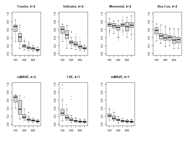
The simulation is performed as follows. We generate 100 i.i.d samples (Yi,𝐗iT)i=1,…,n(Y_{i},{\mathbf{X}}_{i}^{T})_{i=1,...,n} from (29) for each sample size n=100,200,400,600,800,1000n=100,200,400,600,800,1000. Model (29) is a two dimensional model with 𝒮𝔼⁡(Y∣𝐗)=span⁡(𝐛2)⊊𝒮Y|𝐗=span⁡(𝐁)\mathcal{S}_{\mathbb{E}\left(Y\mid{\mathbf{X}}\right)}=\operatorname{span}({\mathbf{b}}_{2})\subsetneq\mathcal{S}_{Y\mid{\mathbf{X}}}=\operatorname{span}({\mathbf{B}}). For methods (I)-(V), we set k=2k=2 and estimate 𝐁∈ℝ10×2{\mathbf{B}}\in{\mathbb{R}}^{10\times 2}. For (VI) and (VII), we set k=1k=1 and estimate 𝐛2∈ℝ10×1{\mathbf{b}}_{2}\in{\mathbb{R}}^{10\times 1}. Then, we calculate errj,n=‖𝐁^​𝐁^T−𝐁𝐁T‖/(2​k)1/2\text{err}_{j,n}=\|\widehat{{\mathbf{B}}}\widehat{{\mathbf{B}}}^{T}-{\mathbf{B}}{\mathbf{B}}^{T}\|/(2k)^{1/2}, j=1,…,100j=1,\ldots,100, n∈{100,200,400,600,800,1000}n\in\{100,200,400,600,800,1000\}. Figure 2 displays the distribution of e​r​rj,nerr_{j,n} for increasing nn for the seven methods. As the sample size increases ECVE Indicator, Fourier and csMAVE are on par with respect to both speed and accuracy. The accuracy of ECVE Box-Cox improves as the sample size increases but at a slower rate. There is no improvement in the accuracy of ECVE monomial. This is not surprising as the monomial, as well as the Box-Cox, do not satisfy the assumption supt∈ΩT|ft​(Y)|<M<∞\sup_{t\in\Omega_{T}}|f_{t}(Y)|<M<\infty in Theorem 11, in contrast to the Indicator and Fourier ensembles. The Fourier, Indicator ECVE and csMAVE estimate 𝒮Y|𝐗=span⁡{𝐁}\mathcal{S}_{Y\mid{\mathbf{X}}}=\operatorname{span}\{{\mathbf{B}}\} consistently and the mean subspace methods, CVE and mMAVE, estimate 𝒮𝔼⁡(Y∣𝐗)=span⁡{𝐛2}\mathcal{S}_{\mathbb{E}\left(Y\mid{\mathbf{X}}\right)}=\operatorname{span}\{{\mathbf{b}}_{2}\} consistently.

Refer to caption
Figure 1: Box plots of the estimation errors over 100100 replications of model (29) with n=300n=300 over m=|ℱ|=(2,4,8,10,26,50,76,100)m=|\mathcal{F}|=(2,4,8,10,26,50,76,100) across four ensembles.
Refer to caption
Figure 2: Estimation error distribution of model (29) plotted over n=(100,200,400,600,800,1000)n=(100,200,400,600,800,1000) for the seven (I-VII) methods

6.3 Evaluating estimation accuracy

We consider seven models, (M1-M7) defined in Table 1, three different sample sizes {100,200,400}\{100,200,400\}, and three different distributions of the predictor vector 𝐗=𝚺1/2​𝐙∈ℝp{\mathbf{X}}=\mbox{\boldmath$\Sigma$}^{1/2}{\mathbf{Z}}\in{\mathbb{R}}^{p}, where 𝚺=(Σi​j)i,j=1,…,p\mbox{\boldmath$\Sigma$}=(\Sigma_{ij})_{i,j=1,\ldots,p}, Σi,j=0.5|i−j|\Sigma_{i,j}=0.5^{|i-j|}. Throughout, p=10p=10, 𝐁{\mathbf{B}} are the first kk columns of 𝐈p{\mathbf{I}}_{p}, and ϵ∼N⁡(0,1)\epsilon\sim N(0,1) independent of 𝐗{\mathbf{X}}. As in [WX08], we consider three distributions for 𝐙∈ℝp{\mathbf{Z}}\in{\mathbb{R}}^{p}: (I) N⁡(0,𝐈p)N(0,{\mathbf{I}}_{p}), (II) pp-dimensional uniform distribution on [−3,3]p[-\sqrt{3},\sqrt{3}]^{p}, i.e. all components of 𝐙{\mathbf{Z}} are independent and uniformly distributed , and (III) a mixture-distribution N⁡(0,𝐈p)+𝝁N(0,{\mathbf{I}}_{p})+\mbox{\boldmath$\mu$}, where 𝝁=(μ1,…,μp)T∈ℝp\mbox{\boldmath$\mu$}=(\mu_{1},\ldots,\mu_{p})^{T}\in{\mathbb{R}}^{p} with μj=2\mu_{j}=2, μk=0\mu_{k}=0, for k≠jk\neq j, and jj is uniformly distributed on {1,…,p}\{1,\ldots,p\}.

The simple and weighted [see Section 4.1] Fourier and Indicator ensembles are used to form four ensemble conditional variance estimators (ECVE). The monomial and BoxCox ensembles were also used but did not give satisfactory results and are not reported. From these two ensembles four ECVE estimators are formed and compared against the reference method csMAVE [WX08], which is implemented in the R package MAVE. The source code for conditional variance estimation and its ensemble version is available at https://git.art-ist.cc/daniel/CVE.

Table 1: Models
Name Model 𝒮𝔼⁡(Y∣𝐗)\mathcal{S}_{\mathbb{E}\left(Y\mid{\mathbf{X}}\right)} 𝒮Y|𝐗\mathcal{S}_{Y\mid{\mathbf{X}}} kk
M1 Y=1𝐛1T​𝐗+0.2​ϵY=\frac{1}{{\mathbf{b}}_{1}^{T}{\mathbf{X}}}+0.2\epsilon span⁡{𝐛1}\operatorname{span}\{{\mathbf{b}}_{1}\} span⁡{𝐛1}\operatorname{span}\{{\mathbf{b}}_{1}\} 1
M2 Y=cos⁡(2​𝐛1T​𝐗)+cos⁡(𝐛2T​𝐗)+0.2​ϵY=\cos(2{\mathbf{b}}_{1}^{T}{\mathbf{X}})+\cos({\mathbf{b}}_{2}^{T}{\mathbf{X}})+0.2\epsilon span⁡{𝐛1,𝐛2}\operatorname{span}\{{\mathbf{b}}_{1},{\mathbf{b}}_{2}\} span⁡{𝐛1,𝐛2}\operatorname{span}\{{\mathbf{b}}_{1},{\mathbf{b}}_{2}\} 2
M3 Y=(𝐛2T​𝐗)+(0.5+(𝐛1T​𝐗)2)​ϵY=({\mathbf{b}}_{2}^{T}{\mathbf{X}})+(0.5+({\mathbf{b}}_{1}^{T}{\mathbf{X}})^{2})\epsilon span⁡{𝐛2}\operatorname{span}\{{\mathbf{b}}_{2}\} span⁡{𝐛1,𝐛2}\operatorname{span}\{{\mathbf{b}}_{1},{\mathbf{b}}_{2}\} 2
M4 Y=𝐛1T​𝐗0.5+(1.5+𝐛2T​𝐗)2+(|𝐛1T​𝐗|+(𝐛2T​𝐗)2+0.5)​ϵY=\frac{{\mathbf{b}}_{1}^{T}{\mathbf{X}}}{0.5+(1.5+{\mathbf{b}}_{2}^{T}{\mathbf{X}})^{2}}+(|{\mathbf{b}}_{1}^{T}{\mathbf{X}}|+({\mathbf{b}}_{2}^{T}{\mathbf{X}})^{2}+0.5)\epsilon span⁡{𝐛1,𝐛2}\operatorname{span}\{{\mathbf{b}}_{1},{\mathbf{b}}_{2}\} span⁡{𝐛1,𝐛2}\operatorname{span}\{{\mathbf{b}}_{1},{\mathbf{b}}_{2}\} 2
M5 Y=𝐛3T​𝐗+sin⁡(𝐛1T​𝐗​(𝐛2T​𝐗)2)​ϵY={\mathbf{b}}_{3}^{T}{\mathbf{X}}+\sin({\mathbf{b}}_{1}^{T}{\mathbf{X}}({\mathbf{b}}_{2}^{T}{\mathbf{X}})^{2})\epsilon span⁡{𝐛3}\operatorname{span}\{{\mathbf{b}}_{3}\} span⁡{𝐛1,𝐛2,𝐛3}\operatorname{span}\{{\mathbf{b}}_{1},{\mathbf{b}}_{2},{\mathbf{b}}_{3}\} 3
M6 Y=0.5​(𝐛1T​𝐗)2​ϵY=0.5({\mathbf{b}}_{1}^{T}{\mathbf{X}})^{2}\epsilon span⁡{𝟎}\operatorname{span}\{{\mathbf{0}}\} span⁡{𝐛1}\operatorname{span}\{{\mathbf{b}}_{1}\} 1
M7 Y=cos⁡(𝐛1T​𝐗−π)+cos⁡(2​𝐛1T​𝐗)​ϵY=\cos({\mathbf{b}}_{1}^{T}{\mathbf{X}}-\pi)+\cos(2{\mathbf{b}}_{1}^{T}{\mathbf{X}})\epsilon span⁡{𝐛1}\operatorname{span}\{{\mathbf{b}}_{1}\} span⁡{𝐛1}\operatorname{span}\{{\mathbf{b}}_{1}\} 1

We set q=p−kq=p-k and generate r=100r=100 replicates of models M1-M7 with the specified distribution of 𝐗{\mathbf{X}} and sample size nn. We estimate 𝐁{\mathbf{B}} using the four ECVE methods and csMAVE. The accuracy of the estimates is assessed using e​r​r=‖𝐏𝐁−𝐏𝐁^‖2/2​k∈[0,1]err=\|\mathbf{P}_{\mathbf{B}}-\mathbf{P}_{\widehat{{\mathbf{B}}}}\|_{2}/\sqrt{2k}\in[0,1], where 𝐏𝐁=𝐁​(𝐁T​𝐁)−1​𝐁T\mathbf{P}_{\mathbf{B}}={\mathbf{B}}({\mathbf{B}}^{T}{\mathbf{B}})^{-1}{\mathbf{B}}^{T} is the orthogonal projection matrix on span⁡{𝐁}\operatorname{span}\{{\mathbf{B}}\}. The factor 2​k\sqrt{2k} normalizes the distance, with values closer to zero indicating better agreement and values closer to one indicating strong disagreement. The results are displayed in Tables 2-8. In M1, which is taken from [WX08], the mean subspace agrees with the central subspace, i.e. 𝒮𝔼⁡(Y∣𝐗)=𝒮Y|𝐗\mathcal{S}_{\mathbb{E}\left(Y\mid{\mathbf{X}}\right)}=\mathcal{S}_{Y\mid{\mathbf{X}}}, but due to the unboundedness of the link function g⁡(x)=1/xg(x)=1/x most mean subspace estimation methods, such as SIR, mean MAVE and CVE, fail. In contrast, all 4 ensemble CVE methods and csMAVE succeed in identifying the minimal dimension reduction subspace, with ensemble CVE performing slightly better, as can be seen in Table 2. In particular, Fourier is the best performing method. M2, is a two dimensional mean subspace model, i.e. 𝒮𝔼⁡(Y∣𝐗)=𝒮Y|𝐗\mathcal{S}_{\mathbb{E}\left(Y\mid{\mathbf{X}}\right)}=\mathcal{S}_{Y\mid{\mathbf{X}}}, and in Table 3 we see that csMAVE is the best performing method. M3 is the same as model (29) and here the mean subspace is a proper subset of the central subspace. In Table 4 we see that Indicator_weighted and csMAVE are the best performers and are roughly on par. In M4, the two dimensional mean subspace, which determines also the heteroskedasticity, agrees with the central subspace. In Table 5 we see that this model is quite challenging for all methods, and only Indicator_weighted and csMAVE give satisfactory results, with Indicator_weighted the clear winner.

In M5, the heteroskedasticity is induced by an interaction term, and the three dimensional central subspace model is a proper superset of the one dimensional mean subspace. In Table 6 we see that M5 is quite challenging for all five methods, therefore we increase the sample size nn to 800800. For M5, the two weighted ensemble conditional variance estimators are the best performing methods followed by csMAVE.

M6 is a one dimensional pure central subspace model, whereas the mean subspace is 00. In Table 7, we see that for n=100n=100 the two weighted ECVEs are the best performing methods and for higher sample sizes csMAVE is slightly more accurate than the ECVE methods.

In M7 the one dimensional mean subspace agrees with the central subspace, i.e. 𝒮𝔼⁡(Y∣𝐗)=𝒮Y|𝐗\mathcal{S}_{\mathbb{E}\left(Y\mid{\mathbf{X}}\right)}=\mathcal{S}_{Y\mid{\mathbf{X}}}, and the conditional first and second moments, 𝔼⁡(Yl∣𝐗)\mathbb{E}(Y^{l}\mid{\mathbf{X}}) for l=1,2l=1,2, are highly nonlinear and periodic functions of the sufficient reduction. In Table 8, we see that all ensemble conditional variance estimators clearly outperform csMAVE.

Table 2: Mean and standard deviation (in parenthesis) of estimation errors of M1
Distribution nn Fourier Fourier_weighted Indicator Indicator_weighted csMAVE
I 100 0.172 0.201 0.248 0.265 0.210
(0.047) (0.054) (0.064) (0.063) (0.063)
I 200 0.120 0.142 0.182 0.197 0.128
(0.029) (0.037) (0.045) (0.049) (0.037)
I 400 0.079 0.091 0.126 0.136 0.080
(0.020) (0.024) (0.037) (0.040) (0.024)
II 100 0.174 0.196 0.241 0.254 0.193
(0.038) (0.049) (0.055) (0.056) (0.059)
II 200 0.110 0.127 0.170 0.182 0.121
(0.031) (0.033) (0.043) (0.045) (0.036)
II 400 0.078 0.091 0.122 0.132 0.079
(0.021) (0.026) (0.031) (0.033) (0.020)
III 100 0.187 0.218 0.256 0.263 0.204
(0.045) (0.053) (0.060) (0.058) (0.066)
III 200 0.118 0.137 0.171 0.179 0.118
(0.031) (0.038) (0.043) (0.042) (0.033)
III 400 0.082 0.101 0.127 0.132 0.079
(0.020) (0.029) (0.031) (0.032) (0.022)
Table 3: Mean and standard deviation (in parenthesis) of estimation errors of M2
Distribution nn Fourier Fourier_weighted Indicator Indicator_weighted csMAVE
I 100 0.670 0.601 0.629 0.582 0.575
(0.089) (0.135) (0.130) (0.140) (0.176)
I 200 0.478 0.388 0.436 0.407 0.219
(0.201) (0.152) (0.193) (0.162) (0.136)
I 400 0.226 0.201 0.231 0.236 0.098
(0.153) (0.074) (0.127) (0.111) (0.025)
II 100 0.663 0.652 0.687 0.658 0.544
(0.097) (0.104) (0.057) (0.080) (0.176)
II 200 0.525 0.468 0.601 0.539 0.182
(0.171) (0.171) (0.127) (0.148) (0.096)
II 400 0.267 0.307 0.375 0.357 0.087
(0.081) (0.146) (0.154) (0.141) (0.021)
III 100 0.657 0.590 0.530 0.542 0.603
(0.104) (0.148) (0.155) (0.148) (0.193)
III 200 0.421 0.367 0.306 0.336 0.240
(0.203) (0.165) (0.147) (0.151) (0.193)
III 400 0.170 0.170 0.144 0.170 0.089
(0.110) (0.071) (0.053) (0.063) (0.019)
Table 4: Mean and standard deviation (in parenthesis) of estimation errors of M3
Distribution nn Fourier Fourier_weighted Indicator Indicator_weighted csMAVE
I 100 0.744 0.657 0.668 0.561 0.602
(0.056) (0.113) (0.083) (0.142) (0.147)
I 200 0.702 0.472 0.559 0.369 0.374
(0.061) (0.177) (0.147) (0.155) (0.148)
I 400 0.621 0.252 0.408 0.223 0.203
(0.148) (0.102) (0.177) (0.064) (0.061)
II 100 0.751 0.698 0.683 0.570 0.635
(0.041) (0.076) (0.080) (0.136) (0.136)
II 200 0.719 0.521 0.584 0.355 0.387
(0.040) (0.163) (0.111) (0.097) (0.144)
II 400 0.686 0.267 0.452 0.252 0.201
(0.079) (0.084) (0.153) (0.052) (0.045)
III 100 0.739 0.676 0.654 0.563 0.571
(0.073) (0.106) (0.105) (0.150) (0.120)
III 200 0.704 0.546 0.523 0.368 0.330
(0.048) (0.162) (0.171) (0.153) (0.131)
III 400 0.616 0.252 0.297 0.202 0.179
(0.151) (0.113) (0.106) (0.055) (0.042)
Table 5: Mean and standard deviation (in parenthesis) of estimation errors of M4
Distribution nn Fourier Fourier_weighted Indicator Indicator_weighted csMAVE
I 100 0.836 0.794 0.774 0.713 0.803
(0.072) (0.076) (0.074) (0.105) (0.087)
I 200 0.820 0.733 0.747 0.545 0.685
(0.066) (0.094) (0.060) (0.150) (0.116)
I 400 0.782 0.633 0.710 0.364 0.534
(0.059) ( 0.142) (0.081) (0.129) (0.155)
II 100 0.839 0.828 0.788 0.751 0.818
(0.067) (0.064) (0.062) (0.095) (0.095)
II 200 0.834 0.781 0.759 0.660 0.701
(0.171) (0.081) (0.040) (0.117) (0.111)
II 400 0.812 0.712 0.739 0.511 0.544
(0.059) (0.097) (0.038) (0.135) (0.151)
III 100 0.838 0.815 0.764 0.706 0.786
(0.074) (0.077) (0.069) (0.108) (0.109)
III 200 0.829 0.761 0.726 0.544 0.676
(0.071) (0.099) (0.083) (0.149) (0.123)
III 400 0.796 0.646 0.669 0.317 0.506
(0.069) (0.139) (0.113) (0.110) (0.146)
Table 6: Mean and standard deviation (in parenthesis) of estimation errors of M5
Distribution nn Fourier Fourier_weighted Indicator Indicator_weighted csMAVE
I 100 0.705 0.682 0.708 0.691 0.709
(0.060) (0.067) (0.060) (0.056) (0.069)
I 200 0.679 0.634 0.688 0.642 0.687
(0.061) (0.054) (0.058) (0.060) (0.073)
I 400 0.644 0.588 0.660 0.591 0.646
(0.050) (0.047) (0.056) (0.061) (0.082)
I 800 0.622 0.543 0.629 0.493 0.553
(0.032) (0.078) (0.035) (0.100) (0.077)
II 100 0.712 0.688 0.713 0.697 0.722
(0.060) (0.069) (0.051) (0.057) (0.054)
II 200 0.693 0.669 0.694 0.669 0.697
(0.058) (0.065) (0.054) (0.057) (0.064)
II 400 0.670 0.614 0.681 0.633 0.687
(0.054) (0.059) (0.052) (0.050) (0.067)
II 800 0.660 0.584 0.672 0.585 0.589
(0.053) (0.045) (0.052) (0.055) (0.074)
III 100 0.706 0.687 0.703 0.691 0.724
(0.062) (0.062) (0.061) (0.061) (0.051)
III 200 0.701 0.655 0.702 0.668 0.703
(0.063) (0.069) (0.058) (0.074) (0.080)
III 400 0.659 0.603 0.664 0.604 0.682
(0.062) (0.072) (0.059) (0.077) (0.081)
III 800 0.657 0.562 0.651 0.513 0.602
(0.064) (0.068) (0.052) (0.109) (0.087)
Table 7: Mean and standard deviation (in parenthesis) of estimation errors of M6
Distribution nn Fourier Fourier_weighted Indicator Indicator_weighted csMAVE
I 100 0.304 0.294 0.492 0.299 0.539
(0.092) (0.082) (0.135) (0.087) (0.255)
I 200 0.217 0.213 0.329 0.205 0.194
(0.057) (0.054) (0.107) (0.059) (0.061)
I 400 0.142 0.146 0.199 0.138 0.114
(0.036) ( 0.035) (0.069) (0.039) (0.034)
II 100 0.308 0.293 0.479 0.299 0.488
(0.094) (0.073) (0.129) (0.086) (0.248)
II 200 0.205 0.210 0.321 0.210 0.192
(0.058) (0.057) (0.095) (0.058) (0.061)
II 400 0.144 0.150 0.190 0.142 0.111
(0.039) (0.042) (0.055) (0.045) (0.032)
III 100 0.373 0.375 0.504 0.322 0.562
(0.152) (0.175) (0.143) (0.083) (0.273)
III 200 0.226 0.230 0.340 0.218 0.218
(0.065) (0.070) (0.100) (0.060) (0.083)
III 400 0.149 0.151 0.194 0.146 0.114
(0.039) (0.038) (0.068) (0.042) (0.032)
Table 8: Mean and standard deviation (in parenthesis) of estimation errors of M7
Distribution nn Fourier Fourier_weighted Indicator Indicator_weighted csMAVE
I 100 0.273 0.237 0.241 0.252 0.790
(0.169) (0.050) (0.136) (0.158) (0.316)
I 200 0.160 0.159 0.143 0.153 0.425
(0.093) (0.041) (0.083) (0.093) (0.391)
I 400 0.098 0.104 0.088 0.102 0.127
(0.024) ( 0.025) (0.021) (0.093) (0.202)
II 100 0.233 0.260 0.236 0.265 0.902
(0.057) (0.134) (0.142) (0.185) (0.219)
II 200 0.154 0.176 0.145 0.150 0.649
(0.058) (0.124) (0.093) (0.094) (0.414)
II 400 0.097 0.110 0.087 0.099 0.295
(0.025) (0.094) (0.022) (0.093) (0.391)
III 100 0.274 0.303 0.238 0.298 0.933
(0.201) (0.237) (0.160) (0.242) (0.163)
III 200 0.167 0.188 0.159 0.167 0.678
(0.120) (0.159) (0.150) (0.144) (0.408)
III 400 0.100 0.116 0.089 0.112 0.375
(0.023) (0.090) (0.023) (0.129) (0.431)

7 Boston Housing Data

We apply the ensemble conditional variance estimator and csMAVE to the Boston Housing data set. This data set has been extensively used as a benchmark for assessing regression methods [see, for example, [JWHT13]], and is available in the R-package mlbench. The data contains 506 instances of 14 variables from the 1970 Boston census, 13 of which are continuous. The binary variable chas, indexing proximity to the Charles river, is omitted from the analysis since ensemble conditional variance estimation operates under the assumption of continuous predictors. The target variable is the median value of owner-occupied homes, medv, in $1,000. The 12 predictors are crim (per capita crime rate by town), zn (proportion of residential land zoned for lots over 25,000 sq.ft), indus (proportion of non-retail business acres per town), nox (nitric oxides concentration (parts per 10 million)), rm (average number of rooms per dwelling), age (proportion of owner-occupied units built prior to 1940), dis (weighted distances to five Boston employment centres), rad (index of accessibility to radial highways), tax (full-value property-tax rate per $10,000), ptratio (pupil-teacher ratio by town), lstat (percentage of lower status of the population), and b stands for 1000​(B−0.63)21000(B-0.63)^{2} where BB is the proportion of blacks by town.

We analyze these data with the weighted and unweighted Fourier and indicator ensembles, and csMAVE. We compute unbiased error estimates by leave-one-out cross-validation. We estimate the sufficient reduction with the five methods from the standardized training set, estimate the forward model from the reduced training set using mars, multivariate adaptive regression splines [Fri91], in the R-package mda, and predict the target variable on the test set. We report results for dimension k=1k=1. The analysis was repeated setting k=2k=2 with similar results. Table 9 reports the first quantile, median, mean and third quantile of the out-of-sample prediction errors. The reductions estimated by the ensemble CVE methods achieve lower mean and median prediction errors than csMAVE. Also, both ensemble CVE and csMAVE are approximately on par with the variable selection methods in [JWHT13, Section 8.3.3].

Table 9: Summary statistics of the out of sample prediction errors for the Boston Housing data obtained by LOO cross validation
Fourier Fourier_weighted Indicator Indicator_weighted csMAVE
25% quantile 0.766 0.785 0.973 0.916 0.851
median 3.323 3.358 3.844 3.666 4.515
mean 19.971 19.948 19.716 19.583 24.309
75% quantile 11.129 10.660 11.099 10.429 16.521

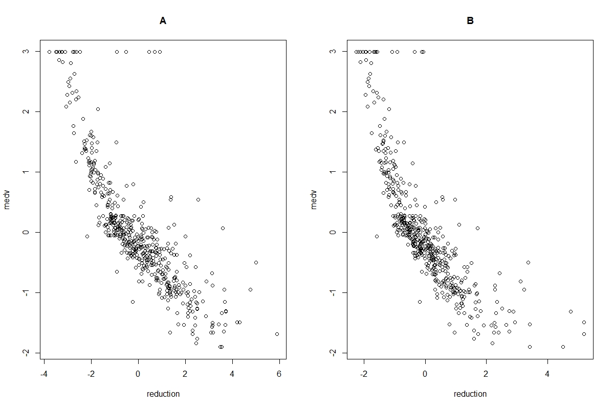
Moreover, we plot the standardized response medv against the reduced Fourier and csMAVE predictors, 𝐁T​𝐗{\mathbf{B}}^{T}{\mathbf{X}}, in Figure 3. The sufficient reductions are estimated using the entire data set. A particular feature of these data is that the response medv appears to be truncated as the highest median price of exactly $50,000 is reported in 16 cases. Both methods pick up similar patterns, which is captured by the relatively high absolute correlation of the coefficients of the two reductions, |𝐁^FourierT​𝐁^csMAVE|=0.786|\widehat{{\mathbf{B}}}_{\texttt{Fourier}}^{T}\widehat{{\mathbf{B}}}_{\texttt{csMAVE}}|=0.786. The coefficients of the reductions, 𝐁^Fourier\widehat{{\mathbf{B}}}_{\texttt{Fourier}} and 𝐁^csMAVE\widehat{{\mathbf{B}}}_{\texttt{csMAVE}}, are reported in Table 10. For the Fourier ensemble, the variables rm and lstat have the highest influence on the target variable medv. This agrees with the analysis in [JWHT13, Section 8.3.4] where it was found that these two variables are by far the most important using different variable selection techniques, such as random forests and boosted regression trees. In contrast, the reduction estimated by csMAVE has a lower coefficient for rm and higher ones for crim and rad.

Table 10: Rounded coefficients of the estimated reductions for 𝐁^Fourier\widehat{{\mathbf{B}}}_{\texttt{Fourier}} and 𝐁^csMAVE\widehat{{\mathbf{B}}}_{\texttt{csMAVE}} from the full Boston Housing data
crim zn indus nox rm age dis rad tax ptratio b lstat
Fourier 0.21 -0.01 0.04 0.1 -0.62 0.16 0.2 0 0.2 0.27 -0.25 0.57
csMAVE 0.5 -0.05 -0.06 0.14 -0.27 0.11 0.24 -0.43 0.3 0.19 -0.15 0.51
Refer to caption
Figure 3: Panel A: YY vs. 𝐁^FourierT​𝐗\widehat{{\mathbf{B}}}_{\texttt{Fourier}}^{T}{\mathbf{X}}. Panel B: YY vs. 𝐁^csMAVET​𝐗\widehat{{\mathbf{B}}}_{\texttt{csMAVE}}^{T}{\mathbf{X}}

8 Discussion

In this paper, we extend the mean subspace conditional variance estimation (CVE) of [FB21] to the ensemble conditional variance estimation (ECVE), which exhaustively estimates the central subspace, by applying the ensemble device introduced by [YL11]. In Section 5 we showed that the new estimator is consistent for the central subspace. The regularity conditions for consistency require the joint distribution of the target variable and predictors, (Y,𝐗T)T(Y,{\mathbf{X}}^{T})^{T}, be sufficiently smooth. They are comparable to those under which the main competitor csMAVE [WX08] is consistent.

We analysed the estimation accuracy of ECVE in Section 6. We found that it is either on par with csMAVE or that it exhibits substantial performance improvement in certain models. We could not characterize the defining features of the models for which the ensemble conditional variance estimation outperforms csMAVE. This is an interesting line of further research together with establishing more theoretical results such as the rate of convergence, estimation of the structural dimension, and the limiting distribution of the estimator.

ECVE identifies the central subspace via the orthogonal complement and thus circumvents the estimation and inversion of the variance matrix of the predictors 𝐗{\mathbf{X}}. This renders the method formally applicable to settings where the sample size nn is small or smaller than pp, the number of predictors, and leads to potential future research.

Throughout, the dimension of the central subspace, k=dim(𝒮Y|𝐗)k=\dim(\mathcal{S}_{Y\mid{\mathbf{X}}}), is assumed to be known. The derivation of asymptotic tests for dimension is technically very challenging due to the lack of closed-form solution and the lack of independence of all quantities in the calculation. The dimension can be estimated via cross-validation, as in [WX08] and [FB21], or information criteria.

Acknowledgements

The authors gratefully acknowledge the support of the Austrian Science Fund (FWF P 30690-N35) and thank Daniel Kapla for his programming assistance. Daniel Kapla also co-authored the CVE R package that implements the proposed method.

References

  • [AC09] Kofi P. Adragni and R. Dennis Cook. Sufficient dimension reduction and prediction in regression. Philosophical Transactions of the Royal Society A: Mathematical, Physical and Engineering Sciences, 367(1906):4385–4405, 11 2009.
  • [Ame85] Takeshi Amemiya. Advanced econometrics. Harvard university press, 1985.
  • [Boo02] W. M. Boothby. An Introduction to Differentiable Manifolds and Riemannian Geometry. Academic Press, 2002.
  • [CD88] William S. Cleveland and Susan J. Devlin. Locally weighted regression: An approach to regression analysis by local fitting. Journal of the American Statistical Association, 83(403):596–610, 1988.
  • [CL02] R.Dennis Cook and Bing Li. Dimension reduction for conditional mean in regression. Ann. Statist., 30(2):455–474, 04 2002.
  • [Coo98] Dennis R. Cook. Regression Graphics: Ideas for studying regressions through graphics. Wiley, New York, 1998.
  • [Coo07] R. Dennis Cook. Fisher lecture: Dimension reduction in regression. Statist. Sci., 22(1):1–26, 02 2007.
  • [Fad85] Arnold M. Faden. The existence of regular conditional probabilities: Necessary and sufficient conditions. The Annals of Probability, 13(1):288–298, 1985.
  • [FB21] Lukas Fertl and Efstathia Bura. Conditional variance estimator for sufficient dimension reduction, 2021.
  • [Fri91] Jerome H. Friedman. Multivariate adaptive regression splines. The Annals of Statistics, 19(1):1–67, 1991.
  • [GH94] Phillip Griffiths and Joseph Harris. Principles of algebraic geometry. Wiley Classics Library. John Wiley & Sons, Inc., New York, 1994. Reprint of the 1978 original.
  • [Han08] Bruce E. Hansen. Uniform convergence rates for kernel estimation with dependent data. Econometric Theory, 24:726–748, 2008.
  • [Heu95] H. Heuser. Analysis 2, 9 Auflage. Teubner, 1995.
  • [Jen69] Robert I. Jennrich. Asymptotic properties of non-linear least squares estimators. Ann. Math. Statist., 40(2):633–643, 04 1969.
  • [JWHT13] Gareth James, Daniela Witten, Trevor Hastie, and Robert Tibshirani. An Introduction to Statistical Learning: with Applications in R. Springer, 2013.
  • [Kar93] Alan F. Karr. Probability. Springer Texts in Statistics. Springer-Verlag New York, 1993.
  • [Li91] K. C. Li. Sliced inverse regression for dimension reduction. Journal of the American Statistical Association, 86(414):316–327, 1991.
  • [Li18] Bing Li. Sufficient dimension reduction: methods and applications with R. CRC Press, Taylor & Francis Group, 2018.
  • [LJFR04] D. Leao Jr., M. Fragoso, and P. Ruffino. Regular conditional probability, disintegration of probability and radon spaces. Proyecciones (Antofagasta), 23:15 – 29, 05 2004.
  • [MMW+63] M.R. Mickey, P.B. Mundle, D.N. Walker, A.M. Glinski, Inc C-E-I-R, and Aerospace Research Laboratories (U.S.). Test Criteria for Pearson Type III Distributions. ARL (Aerospace Research Laboratories (U.S.))). Aerospace Research Laboratories, Office of Aerospace Research, United States Air Force, 1963.
  • [MZ13] Yanyuan Ma and Liping Zhu. A review on dimension reduction. International Statistical Review, 81(1):134–150, 4 2013.
  • [S.N27] S.N.Bernstein. Theory of Probability. 1927.
  • [Tag11] Hemant D. Tagare. Notes on optimization on stiefel manifolds, January 2011.
  • [WX08] Hansheng Wang and Yingcun Xia. Sliced regression for dimension reduction. Journal of the American Statistical Association, 103(482):811–821, 2008.
  • [WY19] Hang Weiqiang and Xia Yingcun. MAVE: Methods for Dimension Reduction, 2019. R package version 1.3.10.
  • [XTLZ02] Yingcun Xia, Howell Tong, W. K. Li, and Li-Xing Zhu. An adaptive estimation of dimension reduction space. Journal of the Royal Statistical Society: Series B (Statistical Methodology), 64(3):363–410, 2002.
  • [YL11] Xiangrong Yin and Bing Li. Sufficient dimension reduction based on an ensemble of minimum average variance estimators. Ann. Statist., 39(6):3392–3416, 12 2011.
  • [YLC08] Xiangrong Yin, Bing Li, and R. Cook. Successive direction extraction for estimating the central subspace in a multiple-index regression. Journal of Multivariate Analysis, 99:1733–1757, 09 2008.
  • [ZZ10] Peng Zeng and Yu Zhu. An integral transform method for estimating the central mean and central subspaces. Journal of Multivariate Analysis, 101(1):271 – 290, 2010.

Appendix

For any 𝐕∈𝒮⁡(p,q){\mathbf{V}}\in{\mathcal{S}}(p,q), defined in (3), we generically denote a basis of the orthogonal complement of its column space span⁡{𝐕}\operatorname{span}\{{\mathbf{V}}\}, by 𝐔{\mathbf{U}}. That is, 𝐔∈𝒮⁡(p,p−q){\mathbf{U}}\in{\mathcal{S}}(p,p-q) such that span⁡{𝐕}⟂span⁡{𝐔}\operatorname{span}\{{\mathbf{V}}\}\perp\operatorname{span}\{{\mathbf{U}}\} and span⁡{𝐕}∪span⁡{𝐔}=ℝp\operatorname{span}\{{\mathbf{V}}\}\cup\operatorname{span}\{{\mathbf{U}}\}={\mathbb{R}}^{p}, 𝐔T​𝐕=𝟎∈ℝ(p−q)×q,𝐔T​𝐔=𝐈p−q{\mathbf{U}}^{T}{\mathbf{V}}={\mathbf{0}}\in{\mathbb{R}}^{(p-q)\times q},{\mathbf{U}}^{T}{\mathbf{U}}={\mathbf{I}}_{p-q}. For any 𝐱,𝐬0∈ℝp{\mathbf{x}},\mathbf{s}_{0}\in{\mathbb{R}}^{p} we can always write

𝐱=𝐬0+𝐏𝐕​(𝐱−𝐬0)+𝐏𝐔​(𝐱−𝐬0)=𝐬0+𝐕𝐫1+𝐔𝐫2{\mathbf{x}}=\mathbf{s}_{0}+\mathbf{P}_{\mathbf{V}}({\mathbf{x}}-\mathbf{s}_{0})+\mathbf{P}_{\mathbf{U}}({\mathbf{x}}-\mathbf{s}_{0})=\mathbf{s}_{0}+{\mathbf{V}}{\mathbf{r}}_{1}+{\mathbf{U}}{\mathbf{r}}_{2} (31)

where 𝐫1=𝐕T​(𝐱−𝐬0)∈ℝq,𝐫2=𝐔T​(𝐱−𝐬0)∈ℝp−q{\mathbf{r}}_{1}={\mathbf{V}}^{T}({\mathbf{x}}-\mathbf{s}_{0})\in{\mathbb{R}}^{q},{\mathbf{r}}_{2}={\mathbf{U}}^{T}({\mathbf{x}}-\mathbf{s}_{0})\in{\mathbb{R}}^{p-q}.

Proof of Theorem 4.

The density of 𝐗|𝐗∈𝐬0+span⁡{𝐕}{\mathbf{X}}\mid{\mathbf{X}}\in\mathbf{s}_{0}+\operatorname{span}\{{\mathbf{V}}\} is given by

f𝐗|𝐗∈𝐬0+span⁡{𝐕}​(𝐫1)=f𝐗​(𝐬0+𝐕𝐫1)∫ℝqf𝐗​(𝐬0+𝐕𝐫)​𝑑𝐫\displaystyle f_{{\mathbf{X}}\mid{\mathbf{X}}\in\mathbf{s}_{0}+\operatorname{span}\{{\mathbf{V}}\}}({\mathbf{r}}_{1})=\frac{f_{\mathbf{X}}(\mathbf{s}_{0}+{\mathbf{V}}{\mathbf{r}}_{1})}{\int_{{\mathbb{R}}^{q}}f_{\mathbf{X}}(\mathbf{s}_{0}+{\mathbf{V}}{\mathbf{r}})d{\mathbf{r}}} (32)

where 𝐗{\mathbf{X}} is the pp-dimensional continuous random covariate vector with density f𝐗​(𝐱)f_{\mathbf{X}}({\mathbf{x}}), 𝐬0∈supp​(f𝐗)⊂ℝp\mathbf{s}_{0}\in\text{supp}(f_{\mathbf{X}})\subset{\mathbb{R}}^{p}, and 𝐕{\mathbf{V}} belongs to the Stiefel manifold 𝒮⁡(p,q){\mathcal{S}}(p,q) defined in (3). Equation (32) follows from Theorem 3.1 of [LJFR04] and the fact that (ℝp,ℬ⁡(ℝp))({\mathbb{R}}^{p},\mathcal{B}({\mathbb{R}}^{p})), where ℬ⁡(ℝp)\mathcal{B}({\mathbb{R}}^{p}) denotes the Borel sets on ℝp{\mathbb{R}}^{p}, is a Polish space, which in turnguarantees the existence of the regular conditional probability of 𝐗|𝐗∈𝐬0+span⁡{𝐕}{\mathbf{X}}\mid{\mathbf{X}}\in\mathbf{s}_{0}+\operatorname{span}\{{\mathbf{V}}\} [see also [Fad85]]. Further, the measure is concentrated on the affine subspace 𝐬0+span⁡{𝐕}⊂ℝp\mathbf{s}_{0}+\operatorname{span}\{{\mathbf{V}}\}\subset{\mathbb{R}}^{p} with density (32), which follows from Definition 8.38, Theorem 8.39 of [Kar93], the orthogonal decomposition (31), and the continuity of f𝐗f_{\mathbf{X}} (E.2).

By assumption (E.1), Y=gcs​(𝐁T​𝐗,ϵ)Y=g_{\textit{cs}}({\mathbf{B}}^{T}{\mathbf{X}},\epsilon) with ϵ⟂⟂𝐗\epsilon\perp\!\!\!\perp{\mathbf{X}}. Assume f∈ℱf\in\mathcal{F} for which assumption (E.4) holds and let 𝐁~\widetilde{{\mathbf{B}}} be a basis of 𝒮𝔼​(ft​(Y)∣𝐗)\mathcal{S}_{\mathbb{E}\left(f_{t}(Y)\mid{\mathbf{X}}\right)}; that is, span⁡{𝐁~}=𝒮𝔼​(ft​(Y)∣𝐗)⊆𝒮Y|𝐗=span⁡{𝐁}\operatorname{span}\{\widetilde{{\mathbf{B}}}\}=\mathcal{S}_{\mathbb{E}\left(f_{t}(Y)\mid{\mathbf{X}}\right)}\subseteq\mathcal{S}_{Y\mid{\mathbf{X}}}=\operatorname{span}\{{\mathbf{B}}\}. By Theorem 3, f⁡(Y)=g⁡(𝐁~T​𝐗)+ϵ~f(Y)=g(\widetilde{{\mathbf{B}}}^{T}{\mathbf{X}})+\tilde{\epsilon}, with 𝔼⁡(ϵ~∣𝐗)=0\mathbb{E}(\tilde{\epsilon}\mid{\mathbf{X}})=0 and gg twice continuously differentiable. Therefore,

L~ℱ​(𝐕,𝐬0,f)=𝕍​ar​(f⁡(Y)∣𝐗∈𝐬0+span⁡{𝐕})\displaystyle\tilde{L}_{\mathcal{F}}({\mathbf{V}},\mathbf{s}_{0},f)=\mathbb{V}\mathrm{ar}\left(f(Y)\mid{\mathbf{X}}\in\mathbf{s}_{0}+\operatorname{span}\{{\mathbf{V}}\}\right)
=𝕍​ar​(g⁡(𝐁~T​𝐗)∣𝐗∈𝐬0+span⁡{𝐕})+2​cov​(ϵ~,g⁡(𝐁~T​𝐗)∣𝐗∈𝐬0+span⁡{𝐕})\displaystyle=\mathbb{V}\mathrm{ar}\left(g(\widetilde{{\mathbf{B}}}^{T}{\mathbf{X}})\mid{\mathbf{X}}\in\mathbf{s}_{0}+\operatorname{span}\{{\mathbf{V}}\}\right)+2\mbox{cov}\left(\tilde{\epsilon},g(\widetilde{{\mathbf{B}}}^{T}{\mathbf{X}})\mid{\mathbf{X}}\in\mathbf{s}_{0}+\operatorname{span}\{{\mathbf{V}}\}\right)
+𝕍​ar​(ϵ~∣𝐗∈𝐬0+span⁡{𝐕})\displaystyle+\mathbb{V}\mathrm{ar}\left(\tilde{\epsilon}\mid{\mathbf{X}}\in\mathbf{s}_{0}+\operatorname{span}\{{\mathbf{V}}\}\right)
=𝕍​ar​(g⁡(𝐁~T​𝐗)∣𝐗∈𝐬0+span⁡{𝐕})+𝕍​ar​(ϵ~∣𝐗∈𝐬0+span⁡{𝐕})\displaystyle=\mathbb{V}\mathrm{ar}\left(g(\widetilde{{\mathbf{B}}}^{T}{\mathbf{X}})\mid{\mathbf{X}}\in\mathbf{s}_{0}+\operatorname{span}\{{\mathbf{V}}\}\right)+\mathbb{V}\mathrm{ar}\left(\tilde{\epsilon}\mid{\mathbf{X}}\in\mathbf{s}_{0}+\operatorname{span}\{{\mathbf{V}}\}\right) (33)

The covariance term in (33) vanishes since

cov​(ϵ~,g⁡(𝐁~T​𝐗)∣𝐗∈𝐬0+span⁡{𝐕})=𝔼⁡(𝔼⁡(ϵ~∣𝐗)⏟=0​g​(𝐁~T​𝐗)∣𝐗∈𝐬0+span⁡{𝐕})\displaystyle\mbox{cov}\left(\tilde{\epsilon},g(\widetilde{{\mathbf{B}}}^{T}{\mathbf{X}})\mid{\mathbf{X}}\in\mathbf{s}_{0}+\operatorname{span}\{{\mathbf{V}}\}\right)=\mathbb{E}\left(\underbrace{\mathbb{E}(\tilde{\epsilon}\mid{\mathbf{X}})}_{=0}g(\widetilde{{\mathbf{B}}}^{T}{\mathbf{X}})\mid{\mathbf{X}}\in\mathbf{s}_{0}+\operatorname{span}\{{\mathbf{V}}\}\right)
−E⁡(g⁡(𝐁~T​𝐗)∣𝐗∈𝐬0+span⁡{𝐕})​𝔼​(𝔼⁡(ϵ~∣𝐗)⏟=0∣𝐗∈𝐬0+span⁡{𝐕})=0\displaystyle-E\left(g(\widetilde{{\mathbf{B}}}^{T}{\mathbf{X}})\mid{\mathbf{X}}\in\mathbf{s}_{0}+\operatorname{span}\{{\mathbf{V}}\}\right)\mathbb{E}\left(\underbrace{\mathbb{E}(\tilde{\epsilon}\mid{\mathbf{X}})}_{=0}\mid{\mathbf{X}}\in\mathbf{s}_{0}+\operatorname{span}\{{\mathbf{V}}\}\right)=0

i.e. the sigma field generated by 𝐗∈𝐬0+span⁡{𝐕}{\mathbf{X}}\in\mathbf{s}_{0}+\operatorname{span}\{{\mathbf{V}}\} is a subset of that generated by 𝐗{\mathbf{X}}. By the same argument and using (32)

𝕍​ar​(ϵ~∣𝐗∈𝐬0+span⁡{𝐕})=𝔼⁡(ϵ~2∣𝐗∈𝐬0+span⁡{𝐕})\displaystyle\mathbb{V}\mathrm{ar}\left(\tilde{\epsilon}\mid{\mathbf{X}}\in\mathbf{s}_{0}+\operatorname{span}\{{\mathbf{V}}\}\right)=\mathbb{E}(\tilde{\epsilon}^{2}\mid{\mathbf{X}}\in\mathbf{s}_{0}+\operatorname{span}\{{\mathbf{V}}\})
=𝔼⁡(𝔼⁡(ϵ~2∣𝐗)∣𝐗∈𝐬0+span⁡{𝐕})=𝔼⁡(h⁡(𝐗)∣𝐗∈𝐬0+span⁡{𝐕})\displaystyle=\mathbb{E}(\mathbb{E}(\tilde{\epsilon}^{2}\mid{\mathbf{X}})\mid{\mathbf{X}}\in\mathbf{s}_{0}+\operatorname{span}\{{\mathbf{V}}\})=\mathbb{E}(h({\mathbf{X}})\mid{\mathbf{X}}\in\mathbf{s}_{0}+\operatorname{span}\{{\mathbf{V}}\})
OPEN=∫supp​(f𝐗)∩ℝqh⁡(𝐬0+𝐕𝐫1)×f𝐗​(𝐬0+𝐕𝐫1)​d​𝐫1/t(0)​(𝐕,𝐬0,f))\displaystyle=\int_{\text{supp}(f_{\mathbf{X}})\cap{\mathbb{R}}^{q}}h(\mathbf{s}_{0}+{\mathbf{V}}{\mathbf{r}}_{1})\times f_{\mathbf{X}}(\mathbf{s}_{0}+{\mathbf{V}}{\mathbf{r}}_{1})d{\mathbf{r}}_{1}/t^{(0)}({\mathbf{V}},\mathbf{s}_{0},f))

where 𝔼⁡(ϵ~2∣𝐗=𝐱)=h⁡(𝐱)\mathbb{E}(\tilde{\epsilon}^{2}\mid{\mathbf{X}}={\mathbf{x}})=h({\mathbf{x}}). Using (32) again for the first term in (33) obtains formula (10) and (13).

To see that (7), (10), and (13) are well defined and continuous, let g~​(𝐕,𝐬0,𝐫)=g​(𝐁T​𝐬0+𝐁T​𝐕𝐫)l​f𝐗​(𝐬0+𝐕𝐫)\tilde{g}({\mathbf{V}},\mathbf{s}_{0},{\mathbf{r}})=g({\mathbf{B}}^{T}\mathbf{s}_{0}+{\mathbf{B}}^{T}{\mathbf{V}}{\mathbf{r}})^{l}f_{\mathbf{X}}(\mathbf{s}_{0}+{\mathbf{V}}{\mathbf{r}}) for l=1,2l=1,2 or g~​(𝐕,𝐬0,𝐫)=h⁡(𝐁T​𝐬0+𝐁T​𝐕𝐫)​f𝐗​(𝐬0+𝐕𝐫)\tilde{g}({\mathbf{V}},\mathbf{s}_{0},{\mathbf{r}})=h({\mathbf{B}}^{T}\mathbf{s}_{0}+{\mathbf{B}}^{T}{\mathbf{V}}{\mathbf{r}})f_{\mathbf{X}}(\mathbf{s}_{0}+{\mathbf{V}}{\mathbf{r}}) (for (13)) which are continuous by assumption. In consequence, the parameter depending integrals (12) and (13) are well defined and continuous if (1) g~(𝐕,𝐬0,⋅)\tilde{g}({\mathbf{V}},\mathbf{s}_{0},\cdot) is integrable for all 𝐕∈𝒮⁡(p,q),𝐬0∈supp​(f𝐗){\mathbf{V}}\in{\mathcal{S}}(p,q),\mathbf{s}_{0}\in\text{supp}(f_{\mathbf{X}}), (2) g~​(⋅,⋅,𝐫)\tilde{g}(\cdot,\cdot,{\mathbf{r}}) is continuous for all 𝐫{\mathbf{r}}, and (3) there exists an integrable dominating function of g~\tilde{g} that does not depend on 𝐕{\mathbf{V}} and 𝐬0\mathbf{s}_{0} [see [Heu95, p. 101]].

Furthermore, for some compact set 𝒦\mathcal{K}, t(l)​(𝐕,𝐬0)=∫𝒦g~​(𝐕,𝐬0,𝐫)​𝑑𝐫t^{(l)}({\mathbf{V}},\mathbf{s}_{0})=\int_{\mathcal{K}}\tilde{g}({\mathbf{V}},\mathbf{s}_{0},{\mathbf{r}})d{\mathbf{r}}, since supp​(f𝐗)\text{supp}(f_{\mathbf{X}}) is compact by (E.2). The function g~​(𝐕,𝐬0,𝐫)\tilde{g}({\mathbf{V}},\mathbf{s}_{0},{\mathbf{r}}) is continuous in all inputs by the continuity of gg (E.4) and f𝐗f_{\mathbf{X}} by (E.2), and therefore it attains a maximum. In consequence, all three conditions are satisfied so that t(l)​(𝐕,𝐬0)t^{(l)}({\mathbf{V}},\mathbf{s}_{0}) is well defined and continuous. By the same argument (13) is well defined and continuous.

Next, μl​(𝐕,𝐬0)=t(l)​(𝐕,𝐬0)/t(0)​(𝐕,𝐬0)\mu_{l}({\mathbf{V}},\mathbf{s}_{0})=t^{(l)}({\mathbf{V}},\mathbf{s}_{0})/t^{(0)}({\mathbf{V}},\mathbf{s}_{0}) is continuous since t(0)​(𝐕,𝐬0)>0t^{(0)}({\mathbf{V}},\mathbf{s}_{0})>0 for all interior points 𝐬0∈supp​(f𝐗)\mathbf{s}_{0}\in\text{supp}(f_{\mathbf{X}}) by the continuity of f𝐗f_{\mathbf{X}}, convexity of the support and 𝚺𝐱>0\mbox{\boldmath$\Sigma$}_{{\mathbf{x}}}>0. Then, L~​(𝐕,𝐬0,f)\tilde{L}({\mathbf{V}},\mathbf{s}_{0},f) in (10) is continuous, which results in (8) also being well defined and continuous by virtue of it being a parameter depending integral following the same arguments as above. Moreover, (14) exists as the minimizer of a continuous function over the compact set 𝒮⁡(p,q){\mathcal{S}}(p,q).

Then, (8) can be writen as

Lℱ∗​(𝐕,f)=𝔼𝐬0∼𝐗​(μ2​(𝐕,𝐬0,f)−μ1​(𝐕,𝐬0,f)2)+𝔼𝐬0∼𝐗​(𝕍​ar​(ϵ~∣𝐗∈𝐬0+span⁡{𝐕}))\displaystyle L_{\mathcal{F}}^{*}({\mathbf{V}},f)=\mathbb{E}_{\mathbf{s}_{0}\sim{\mathbf{X}}}\left(\mu_{2}({\mathbf{V}},\mathbf{s}_{0},f)-\mu_{1}({\mathbf{V}},\mathbf{s}_{0},f)^{2}\right)+\mathbb{E}_{\mathbf{s}_{0}\sim{\mathbf{X}}}\left(\mathbb{V}\mathrm{ar}\left(\tilde{\epsilon}\mid{\mathbf{X}}\in\mathbf{s}_{0}+\operatorname{span}\{{\mathbf{V}}\}\right)\right) (34)

where 𝐬0∼𝐗\mathbf{s}_{0}\sim{\mathbf{X}} signifies that 𝐬0\mathbf{s}_{0} is distributed as 𝐗{\mathbf{X}} and the expectation is with respect to the distribution of 𝐬0\mathbf{s}_{0}.

It now suffices to show that the second term on the right hand side of (34) is constant with respect to 𝐕{\mathbf{V}}. By the law of total variance,

𝕍​ar​(ϵ~)\displaystyle\mathbb{V}\mathrm{ar}(\tilde{\epsilon}) =𝔼⁡(𝕍​ar​(ϵ~∣𝐗∈𝐬0+span⁡{𝐕}))+𝕍​ar​(𝔼⁡(ϵ~∣𝐗∈𝐬0+span⁡{𝐕}))\displaystyle=\mathbb{E}\left(\mathbb{V}\mathrm{ar}(\tilde{\epsilon}\mid{\mathbf{X}}\in\mathbf{s}_{0}+\operatorname{span}\{{\mathbf{V}}\})\right)+\mathbb{V}\mathrm{ar}\left(\mathbb{E}(\tilde{\epsilon}\mid{\mathbf{X}}\in\mathbf{s}_{0}+\operatorname{span}\{{\mathbf{V}}\})\right)
=𝔼⁡(𝕍​ar​(ϵ~∣𝐗∈𝐬0+span⁡{𝐕}))\displaystyle=\mathbb{E}\left(\mathbb{V}\mathrm{ar}(\tilde{\epsilon}\mid{\mathbf{X}}\in\mathbf{s}_{0}+\operatorname{span}\{{\mathbf{V}}\})\right) (35)

since 𝔼⁡(ϵ~∣𝐗∈𝐬0+span⁡{𝐕})=𝔼⁡(𝔼⁡(ϵ~∣𝐗)⏟=0∣𝐗∈𝐬0+span⁡{𝐕})=0\mathbb{E}(\tilde{\epsilon}\mid{\mathbf{X}}\in\mathbf{s}_{0}+\operatorname{span}\{{\mathbf{V}}\})=\mathbb{E}(\underbrace{\mathbb{E}(\tilde{\epsilon}\mid{\mathbf{X}})}_{=0}\mid{\mathbf{X}}\in\mathbf{s}_{0}+\operatorname{span}\{{\mathbf{V}}\})=0. Inserting (35) into (34) obtains

Lℱ∗​(𝐕,ft)=𝔼⁡(μ2​(𝐕,𝐗,ft)−μ1​(𝐕,𝐗,ft)2)+𝕍​ar​(ϵ~)\displaystyle L_{\mathcal{F}}^{*}({\mathbf{V}},f_{t})=\mathbb{E}\left(\mu_{2}({\mathbf{V}},{\mathbf{X}},f_{t})-\mu_{1}({\mathbf{V}},{\mathbf{X}},f_{t})^{2}\right)+\mathbb{V}\mathrm{ar}(\tilde{\epsilon})
=𝔼𝐬0∼𝐗​(𝕍​ar​(g⁡(𝐁~T​𝐗)∣𝐗∈𝐬0+span⁡{𝐕}))+𝕍​ar​(ϵ~)\displaystyle=\mathbb{E}_{\mathbf{s}_{0}\sim{\mathbf{X}}}\left(\mathbb{V}\mathrm{ar}\left(g(\widetilde{{\mathbf{B}}}^{T}{\mathbf{X}})\mid{\mathbf{X}}\in\mathbf{s}_{0}+\operatorname{span}\{{\mathbf{V}}\}\right)\right)+\mathbb{V}\mathrm{ar}(\tilde{\epsilon}) (36)

Next we show that (8), or, equivalently (36)), attains its minimum at 𝐕⟂𝐁~{\mathbf{V}}\perp\widetilde{{\mathbf{B}}}. Let 𝐬0∈supp​(f𝐗)\mathbf{s}_{0}\in\text{supp}(f_{\mathbf{X}}) and 𝐕=(𝐯1,…,𝐯q)∈ℝp×q{\mathbf{V}}=(\mathbf{v}_{1},...,\mathbf{v}_{q})\in{\mathbb{R}}^{p\times q}, so that 𝐯u∈span⁡{𝐁}\mathbf{v}_{u}\in\operatorname{span}\{{\mathbf{B}}\} for some u∈{1,…,q}u\in\{1,...,q\}. Since 𝐗∈𝐬0+span⁡{𝐕}⟺𝐗=𝐬0+𝐏𝐕​(𝐗−𝐬0){\mathbf{X}}\in\mathbf{s}_{0}+\operatorname{span}\{{\mathbf{V}}\}\Longleftrightarrow{\mathbf{X}}=\mathbf{s}_{0}+\mathbf{P}_{{\mathbf{V}}}({\mathbf{X}}-\mathbf{s}_{0}), by the first term in (36)

𝕍​ar​(g⁡(𝐁~T​𝐗)∣𝐗∈𝐬0+span⁡{𝐕})=𝕍​ar​(g⁡(𝐁~T​𝐗)∣𝐗=𝐬0+𝐕𝐕T​(𝐗−𝐬0))\displaystyle\mathbb{V}\mathrm{ar}\left(g(\widetilde{{\mathbf{B}}}^{T}{\mathbf{X}})\mid{\mathbf{X}}\in\mathbf{s}_{0}+\operatorname{span}\{{\mathbf{V}}\}\right)=\mathbb{V}\mathrm{ar}\left(g(\widetilde{{\mathbf{B}}}^{T}{\mathbf{X}})\mid{\mathbf{X}}=\mathbf{s}_{0}+{\mathbf{V}}{\mathbf{V}}^{T}({\mathbf{X}}-\mathbf{s}_{0})\right)
=𝕍​ar​(g⁡(𝐁~T​𝐬0+𝐁~T​𝐕𝐕T​(𝐗−𝐬0))∣𝐗=𝐬0+𝐕𝐕T​(𝐗−𝐬0))≥0\displaystyle=\mathbb{V}\mathrm{ar}\left(g(\widetilde{{\mathbf{B}}}^{T}\mathbf{s}_{0}+\widetilde{{\mathbf{B}}}^{T}{\mathbf{V}}{\mathbf{V}}^{T}({\mathbf{X}}-\mathbf{s}_{0}))\mid{\mathbf{X}}=\mathbf{s}_{0}+{\mathbf{V}}{\mathbf{V}}^{T}({\mathbf{X}}-\mathbf{s}_{0})\right)\geq 0 (37)

If (37) is positive, i.e. 𝐁~T​𝐕𝐕T​(𝐗−𝐬0)≠0\widetilde{{\mathbf{B}}}^{T}{\mathbf{V}}{\mathbf{V}}^{T}({\mathbf{X}}-\mathbf{s}_{0})\neq 0 with positive probability, then the lower bound is not attained. If it is zero; i.e., for 𝐕{\mathbf{V}} such that 𝐕{\mathbf{V}} and 𝐁~T\widetilde{{\mathbf{B}}}^{T} are orthogonal, then Lℱ∗​(𝐕,f)=𝕍​ar​(ϵ~)L_{\mathcal{F}}^{*}({\mathbf{V}},f)=\mathbb{V}\mathrm{ar}(\tilde{\epsilon}). Since 𝐬0\mathbf{s}_{0} is arbitrary yet constant, the same inequality holds for (8); that is, (8) attains its minimum for 𝐕{\mathbf{V}} such that 𝐕{\mathbf{V}} and 𝐁~T\widetilde{{\mathbf{B}}}^{T} are orthogonal. Since span⁡{𝐁~T}=𝒮𝔼​(ft​(Y)∣𝐗)\operatorname{span}\{\widetilde{{\mathbf{B}}}^{T}\}=\mathcal{S}_{\mathbb{E}\left(f_{t}(Y)\mid{\mathbf{X}}\right)}, (14) follows. ∎

Proof of Theorem 6.

Under assumptions (E.1), (E.2), and (E.3), (7) is well defined and continuous by arguments analogous to those in the proof of Theorem 4. Therefore (17) exists as a minimizer of a continuous function over the compact set 𝒮⁡(p,q){\mathcal{S}}(p,q).

To show 𝒮Y|𝐗=span⁡{𝐕q}⟂\mathcal{S}_{Y\mid{\mathbf{X}}}=\operatorname{span}\{{\mathbf{V}}_{q}\}^{\perp}, let 𝒮~≠𝒮Y|𝐗\tilde{{\mathcal{S}}}\neq\mathcal{S}_{Y\mid{\mathbf{X}}} with dim(𝒮~)=dim(𝒮Y|𝐗)=k\dim(\tilde{{\mathcal{S}}})=\dim(\mathcal{S}_{Y\mid{\mathbf{X}}})=k. Also, let 𝐙∈ℝp×(p−k){\mathbf{Z}}\in{\mathbb{R}}^{p\times(p-k)} be an orthonormal base of 𝒮~⟂\tilde{{\mathcal{S}}}^{\perp}. Suppose Lℱ​(𝐙)=minV∈𝒮⁡(p,p−k)⁡Lℱ​(𝐕)L_{\mathcal{F}}({\mathbf{Z}})=\min_{V\in{\mathcal{S}}(p,p-k)}L_{\mathcal{F}}({\mathbf{V}}). By (14) and (15) in Theorem 4, Lℱ∗​(𝐕,ft)L_{\mathcal{F}}^{*}({\mathbf{V}},f_{t}), considered as a function from ℝp×(p−kt){\mathbb{R}}^{p\times(p-k_{t})}, is minimized by an orthonormal base of 𝒮𝔼​(ft​(Y)∣𝐗)⟂\mathcal{S}_{\mathbb{E}\left(f_{t}(Y)\mid{\mathbf{X}}\right)}^{\perp} with p−ktp-k_{t} elements, where kt=dim(𝒮𝔼​(ft​(Y)∣𝐗))≤kk_{t}=\dim(\mathcal{S}_{\mathbb{E}\left(f_{t}(Y)\mid{\mathbf{X}}\right)})\leq k. By (E.1), 𝒮𝔼​(ft​(Y)∣𝐗)⊆𝒮Y|𝐗=span⁡{𝐁}\mathcal{S}_{\mathbb{E}\left(f_{t}(Y)\mid{\mathbf{X}}\right)}\subseteq\mathcal{S}_{Y\mid{\mathbf{X}}}=\operatorname{span}\{{\mathbf{B}}\}. As in the proof of Theorem 4, we obtain that Lℱ∗​(𝐕,ft)L_{\mathcal{F}}^{*}({\mathbf{V}},f_{t}), as a function from ℝp×(p−k){\mathbb{R}}^{p\times(p-k)}, is minimized by an orthonormal base 𝐔∈ℝp×(p−k){\mathbf{U}}\in{\mathbb{R}}^{p\times(p-k)} of span⁡{𝐁}⟂\operatorname{span}\{{\mathbf{B}}\}^{\perp}.

Since 𝒮~=span⁡{𝐙}≠span⁡{𝐔}=𝒮Y|𝐗\tilde{{\mathcal{S}}}=\operatorname{span}\{{\mathbf{Z}}\}\neq\operatorname{span}\{{\mathbf{U}}\}=\mathcal{S}_{Y\mid{\mathbf{X}}}, we can rearrange the bases 𝐔=(𝐔1,𝐔2){\mathbf{U}}=({\mathbf{U}}_{1},{\mathbf{U}}_{2}) and 𝐙=(𝐙1,𝐙2){\mathbf{Z}}=({\mathbf{Z}}_{1},{\mathbf{Z}}_{2}) such that span⁡{𝐔1}=span⁡{𝐙1}\operatorname{span}\{{\mathbf{U}}_{1}\}=\operatorname{span}\{{\mathbf{Z}}_{1}\} and span⁡{𝐔2}≠span⁡{𝐙2}\operatorname{span}\{{\mathbf{U}}_{2}\}\neq\operatorname{span}\{{\mathbf{Z}}_{2}\}. Since ℱ\mathcal{F} characterises 𝒮Y|𝐗\mathcal{S}_{Y\mid{\mathbf{X}}}, the set A={t∈ΩT:span⁡{𝐔2}⊆𝒮𝔼​(ft​(Y)∣𝐗)}A=\{t\in\Omega_{T}:\operatorname{span}\{{\mathbf{U}}_{2}\}\subseteq\mathcal{S}_{\mathbb{E}\left(f_{t}(Y)\mid{\mathbf{X}}\right)}\} is non empty and by (E.3) AA is not a null set with respect to the probability measure FTF_{T}.

Thus,

minV∈𝒮⁡(p,p−k)⁡Lℱ​(𝐕)=Lℱ​(𝐙)=𝔼t∼FT​(Lℱ∗​(𝐙,ft))\displaystyle\min_{V\in{\mathcal{S}}(p,p-k)}L_{\mathcal{F}}({\mathbf{V}})=L_{\mathcal{F}}({\mathbf{Z}})=\mathbb{E}_{t\sim F_{T}}\left(L_{\mathcal{F}}^{*}({\mathbf{Z}},f_{t})\right)
=∫ALℱ∗​(𝐙,ft)⏟>Lℱ∗​(𝐔,ft)​d​FT​(t)+∫AcLℱ∗​(𝐙,ft)⏟=Lℱ∗​(𝐔,ft)​d​FT​(t)>𝔼t∼FT​(Lℱ∗​(𝐔,ft)),\displaystyle=\int_{A}\underbrace{L_{\mathcal{F}}^{*}({\mathbf{Z}},f_{t})}_{>L_{\mathcal{F}}^{*}({\mathbf{U}},f_{t})}dF_{T}(t)+\int_{A^{c}}\underbrace{L_{\mathcal{F}}^{*}({\mathbf{Z}},f_{t})}_{=L_{\mathcal{F}}^{*}({\mathbf{U}},f_{t})}dF_{T}(t)>\mathbb{E}_{t\sim F_{T}}\left(L_{\mathcal{F}}^{*}({\mathbf{U}},f_{t})\right),

which contradicts our assumption that Lℱ​(𝐙)=minV∈𝒮⁡(p,p−k)⁡Lℱ​(𝐕)L_{\mathcal{F}}({\mathbf{Z}})=\min_{V\in{\mathcal{S}}(p,p-k)}L_{\mathcal{F}}({\mathbf{V}}). ∎

Next we introduce notation and auxiliary lemmas for the proof of Theorem 8. We suppose all assumptions of Theorem 8 hold. We generically use the letter “C” to denote constants.

Suppose ff is an arbitrary element of ℱ\mathcal{F} and let

Y~i=f⁡(Yi)=g⁡(𝐁~T​𝐗i)+ϵi~\displaystyle\tilde{Y}_{i}=f(Y_{i})=g(\widetilde{{\mathbf{B}}}^{T}{\mathbf{X}}_{i})+\tilde{\epsilon_{i}} (38)

with span⁡{𝐁~}=𝒮𝔼⁡(Y~∣𝐗)=𝒮𝔼⁡(f⁡(Y)∣𝐗)\operatorname{span}\{\widetilde{{\mathbf{B}}}\}={\mathcal{S}}_{\mathbb{E}(\tilde{Y}\mid{\mathbf{X}})}={\mathcal{S}}_{\mathbb{E}(f(Y)\mid{\mathbf{X}})}. Condition (E.4) yields that gg is twice continuously differentiable, and 𝔼⁡(|Y~|8)<∞\mathbb{E}(|\tilde{Y}|^{8})<\infty. Since ff is fixed, we suppress it in t(l)​(𝐕,𝐬0,f)t^{(l)}({\mathbf{V}},\mathbf{s}_{0},f) and h~​(𝐕,𝐬0,f)\tilde{h}({\mathbf{V}},\mathbf{s}_{0},f), so that

tn(l)​(𝐕,𝐬0,f)=tn(l)​(𝐕,𝐬0)=1n​hn(p−q)/2​∑i=1nK⁡(di​(𝐕,𝐬0)hn)​Y~il,\displaystyle t^{(l)}_{n}({\mathbf{V}},\mathbf{s}_{0},f)=t^{(l)}_{n}({\mathbf{V}},\mathbf{s}_{0})=\frac{1}{nh_{n}^{(p-q)/2}}\sum_{i=1}^{n}K\left(\frac{d_{i}({\mathbf{V}},\mathbf{s}_{0})}{h_{n}}\right)\tilde{Y}^{l}_{i}, (39)

which is the sample version of (12) for l=0,1,2l=0,1,2. Eqn. (21) can be expressed as

y¯l​(𝐕,𝐬0)\displaystyle\bar{y}_{l}({\mathbf{V}},\mathbf{s}_{0}) =tn(l)​(𝐕,𝐬0)tn(0)​(𝐕,𝐬0),\displaystyle=\frac{t^{(l)}_{n}({\mathbf{V}},\mathbf{s}_{0})}{t^{(0)}_{n}({\mathbf{V}},\mathbf{s}_{0})}, (40)
Lemma 12.

Assume (E.2) and (K.1) hold. For a continuous function gg, we let Zn​(𝐕,𝐬0)=(∑ig​(𝐗i)l​K​(di​(𝐕,𝐬0)/hn))/(n​hn(p−q)/2)Z_{n}({\mathbf{V}},\mathbf{s}_{0})=\left(\sum_{i}g({\mathbf{X}}_{i})^{l}K(d_{i}({\mathbf{V}},\mathbf{s}_{0})/h_{n})\right)/(nh_{n}^{(p-q)/2}). Then,

𝔼⁡(Zn​(𝐕,𝐬0))\displaystyle\mathbb{E}\left(Z_{n}({\mathbf{V}},\mathbf{s}_{0})\right) =∫supp​(f𝐗)∩ℝp−qK⁡(‖𝐫2‖2)​∫supp​(f𝐗)∩ℝqg~​(𝐫1,hn1/2​𝐫2)​d​𝐫1​d​𝐫2\displaystyle=\int_{\text{supp}(f_{\mathbf{X}})\cap{\mathbb{R}}^{p-q}}K(\|{\mathbf{r}}_{2}\|^{2})\int_{\text{supp}(f_{\mathbf{X}})\cap{\mathbb{R}}^{q}}\tilde{g}({\mathbf{r}}_{1},h_{n}^{1/2}{\mathbf{r}}_{2})d{\mathbf{r}}_{1}d{\mathbf{r}}_{2}

where g~​(𝐫1,𝐫2)=g​(𝐬0+𝐕𝐫1+𝐔𝐫2)l​f𝐗​(𝐬0+𝐕𝐫1+𝐔𝐫2)\tilde{g}({\mathbf{r}}_{1},{\mathbf{r}}_{2})=g(\mathbf{s}_{0}+{\mathbf{V}}{\mathbf{r}}_{1}+{\mathbf{U}}{\mathbf{r}}_{2})^{l}f_{\mathbf{X}}(\mathbf{s}_{0}+{\mathbf{V}}{\mathbf{r}}_{1}+{\mathbf{U}}{\mathbf{r}}_{2}), 𝐱=𝐬0+𝐕𝐫1+𝐔𝐫2{\mathbf{x}}=\mathbf{s}_{0}+{\mathbf{V}}{\mathbf{r}}_{1}+{\mathbf{U}}{\mathbf{r}}_{2} in (31).

Proof of Lemma 12.

By (31), ‖𝐏𝐔​(𝐱−𝐬0)‖2=‖𝐔𝐫2‖2=‖𝐫2‖2\|\mathbf{P}_{{\mathbf{U}}}({\mathbf{x}}-\mathbf{s}_{0})\|^{2}=\|{\mathbf{U}}{\mathbf{r}}_{2}\|^{2}=\|{\mathbf{r}}_{2}\|^{2}. Further

𝔼⁡(Zn​(𝐕,𝐬0))=1hn(p−q)/2​∫supp​(f𝐗)g​(𝐱)l​K​(‖𝐏𝐔​(𝐱−𝐬0)/hn1/2‖2)​f𝐗​(𝐱)​𝑑𝐱\displaystyle\mathbb{E}\left(Z_{n}({\mathbf{V}},\mathbf{s}_{0})\right)=\frac{1}{h_{n}^{(p-q)/2}}\int_{\text{supp}(f_{\mathbf{X}})}g({\mathbf{x}})^{l}K(\|\mathbf{P}_{\mathbf{U}}({\mathbf{x}}-\mathbf{s}_{0})/h^{1/2}_{n}\|^{2})f_{\mathbf{X}}({\mathbf{x}})d{\mathbf{x}}
=1hn(p−q)/2∫supp​(f𝐗)∩ℝp−q∫supp​(f𝐗)∩ℝqg(𝐬0+𝐕𝐫1+𝐔𝐫2)lK(∥𝐫2/hn1/2∥2)×\displaystyle=\frac{1}{h_{n}^{(p-q)/2}}\int_{\text{supp}(f_{\mathbf{X}})\cap{\mathbb{R}}^{p-q}}\int_{\text{supp}(f_{\mathbf{X}})\cap{\mathbb{R}}^{q}}g(\mathbf{s}_{0}+{\mathbf{V}}{\mathbf{r}}_{1}+{\mathbf{U}}{\mathbf{r}}_{2})^{l}K(\|{\mathbf{r}}_{2}/h^{1/2}_{n}\|^{2})\times
f𝐗​(𝐬0+𝐕𝐫1+𝐔𝐫2)​d​𝐫1​d​𝐫2\displaystyle f_{\mathbf{X}}(\mathbf{s}_{0}+{\mathbf{V}}{\mathbf{r}}_{1}+{\mathbf{U}}{\mathbf{r}}_{2})d{\mathbf{r}}_{1}d{\mathbf{r}}_{2}
=∫supp​(f𝐗)∩ℝp−qK⁡(‖𝐫2‖2)​∫supp​(f𝐗)∩ℝqg​(𝐬0+𝐕𝐫1+hn1/2​𝐔𝐫2)l​f𝐗​(𝐬0+𝐕𝐫1+hn1/2​𝐔𝐫2)​d​𝐫1​d​𝐫2\displaystyle=\int_{\text{supp}(f_{\mathbf{X}})\cap{\mathbb{R}}^{p-q}}K(\|{\mathbf{r}}_{2}\|^{2})\int_{\text{supp}(f_{\mathbf{X}})\cap{\mathbb{R}}^{q}}g(\mathbf{s}_{0}+{\mathbf{V}}{\mathbf{r}}_{1}+h_{n}^{1/2}{\mathbf{U}}{\mathbf{r}}_{2})^{l}f_{\mathbf{X}}(\mathbf{s}_{0}+{\mathbf{V}}{\mathbf{r}}_{1}+h_{n}^{1/2}{\mathbf{U}}{\mathbf{r}}_{2})d{\mathbf{r}}_{1}d{\mathbf{r}}_{2}

where the substitution 𝐫~2=𝐫2/hn1/2\tilde{{\mathbf{r}}}_{2}={\mathbf{r}}_{2}/h_{n}^{1/2}, d​𝐫2=hn(p−q)/2​d​𝐫~2d{\mathbf{r}}_{2}=h_{n}^{(p-q)/2}d\tilde{{\mathbf{r}}}_{2} was used to obtain the last equality. ∎

Lemma 13.

Assume (E.1), (E.2), (E.3), (E.4), (H.1) and (K.1) hold. Then, there exists a constant C>0C>0, such that

𝕍​ar​(n​hn(p−q)/2​tn(l)​(𝐕,𝐬0,f))≤n​hn(p−q)/2​C\mathbb{V}\mathrm{ar}\left(nh_{n}^{(p-q)/2}t^{(l)}_{n}({\mathbf{V}},\mathbf{s}_{0},f)\right)\leq nh_{n}^{(p-q)/2}C

for n>n⋆n>n^{\star} and tn(l)​(𝐕,𝐬0)t^{(l)}_{n}({\mathbf{V}},\mathbf{s}_{0}), l=0,1,2l=0,1,2, in (39).

Proof of Lemma 13.

Since a continuous function attains a finite maximum over a compact set, sup𝐱∈supp​(f𝐗)|g⁡(𝐁~T​𝐱)|<∞.\sup_{{\mathbf{x}}\in\text{supp}(f_{\mathbf{X}})}|g(\widetilde{{\mathbf{B}}}^{T}{\mathbf{x}})|<\infty. Therefore,

|Y~i|≤|g⁡(𝐁~T​𝐗i)|+|ϵi~|≤sup𝐱∈supp​(f𝐗)|g⁡(𝐁~T​𝐱)|+|ϵi~|=C+|ϵi~|\displaystyle|\tilde{Y}_{i}|\leq|g(\widetilde{{\mathbf{B}}}^{T}{\mathbf{X}}_{i})|+|\tilde{\epsilon_{i}}|\leq\sup_{{\mathbf{x}}\in\text{supp}(f_{\mathbf{X}})}|g(\widetilde{{\mathbf{B}}}^{T}{\mathbf{x}})|+|\tilde{\epsilon_{i}}|=C+|\tilde{\epsilon_{i}}|

and |Y~i|2​l≤∑u=02​l(2​lu)​Cu​|ϵi~|2​l−u|\tilde{Y}_{i}|^{2l}\leq\sum_{u=0}^{2l}\binom{2l}{u}C^{u}|\tilde{\epsilon_{i}}|^{2l-u}. Since (Y~i,𝐗i)(\tilde{Y}_{i},{\mathbf{X}}_{i}) are i.i.d.,

𝕍​ar​(n​hn(p−q)/2​tn(l)​(𝐕,𝐬0,f))=n​𝕍​ar​(Y~l​K​(di​(𝐕,𝐬0)hn))≤n​𝔼​(Y~2​l​K2​(di​(𝐕,𝐬0)hn))\displaystyle\mathbb{V}\mathrm{ar}\left(nh_{n}^{(p-q)/2}t^{(l)}_{n}({\mathbf{V}},\mathbf{s}_{0},f)\right)=n\mathbb{V}\mathrm{ar}\left(\tilde{Y}^{l}K\left(\frac{d_{i}({\mathbf{V}},\mathbf{s}_{0})}{h_{n}}\right)\right)\leq n\mathbb{E}\left(\tilde{Y}^{2l}K^{2}\left(\frac{d_{i}({\mathbf{V}},\mathbf{s}_{0})}{h_{n}}\right)\right)
=n​𝔼​(|Y~|2​l​K2​(di​(𝐕,𝐬0)hn))≤n​∑u=02​l(2​lu)​Cu​𝔼​(|ϵi~|2​l−u​K2​(di​(𝐕,𝐬0)hn))\displaystyle=n\mathbb{E}\left(|\tilde{Y}|^{2l}K^{2}\left(\frac{d_{i}({\mathbf{V}},\mathbf{s}_{0})}{h_{n}}\right)\right)\leq n\sum_{u=0}^{2l}\binom{2l}{u}C^{u}\mathbb{E}\left(|\tilde{\epsilon_{i}}|^{2l-u}K^{2}\left(\frac{d_{i}({\mathbf{V}},\mathbf{s}_{0})}{h_{n}}\right)\right)
=n​∑u=02​l(2​lu)​Cu​𝔼​(𝔼⁡(|ϵi~|2​l−u∣𝐗i)​K2​(di​(𝐕,𝐬0)hn))\displaystyle=n\sum_{u=0}^{2l}\binom{2l}{u}C^{u}\mathbb{E}\left(\mathbb{E}(|\tilde{\epsilon_{i}}|^{2l-u}\mid{\mathbf{X}}_{i})K^{2}\left(\frac{d_{i}({\mathbf{V}},\mathbf{s}_{0})}{h_{n}}\right)\right) (41)

for l=0,1,2l=0,1,2. Let 𝔼⁡(|ϵi~|2​l−u∣𝐗i)=g2​l−u​(𝐗i)\mathbb{E}(|\tilde{\epsilon_{i}}|^{2l-u}\mid{\mathbf{X}}_{i})=g_{2l-u}({\mathbf{X}}_{i}) for a continuous (by assumption) function g2​l−u​(⋅)g_{2l-u}(\cdot) with finite moments for l=0,1,2l=0,1,2 by the compactness of supp​(f𝐗)\text{supp}(f_{\mathbf{X}}). Using Lemma 12 with

Zn​(𝐕,𝐬0)=1n​hn(p−q)/2​∑ig2​l−u​(𝐗i)​K2​(di​(𝐕,𝐬0)/hn),Z_{n}({\mathbf{V}},\mathbf{s}_{0})=\frac{1}{nh_{n}^{(p-q)/2}}\sum_{i}g_{2l-u}({\mathbf{X}}_{i})K^{2}\left(d_{i}({\mathbf{V}},\mathbf{s}_{0})/h_{n}\right),

where K2​(⋅)K^{2}(\cdot) fulfills (K.1), we calculate

𝔼⁡(𝔼⁡(|ϵi~|2​l−u∣𝐗i)​K2​(di​(𝐕,𝐬0)hn))=hn(p−q)/2​𝔼​(Zn​(𝐕,𝐬0))\displaystyle\mathbb{E}\left(\mathbb{E}(|\tilde{\epsilon_{i}}|^{2l-u}\mid{\mathbf{X}}_{i})K^{2}\left(\frac{d_{i}({\mathbf{V}},\mathbf{s}_{0})}{h_{n}}\right)\right)=h_{n}^{(p-q)/2}\mathbb{E}(Z_{n}({\mathbf{V}},\mathbf{s}_{0}))
=hn(p−q)/2∫supp​(f𝐗)∩ℝp−qK2(∥𝐫2∥2)×\displaystyle=h_{n}^{(p-q)/2}\int_{\text{supp}(f_{\mathbf{X}})\cap{\mathbb{R}}^{p-q}}K^{2}(\|{\mathbf{r}}_{2}\|^{2})\times
∫supp​(f𝐗)∩ℝqg2​l−u​(𝐬0+𝐕𝐫1+hn1/2​𝐔𝐫2)​f𝐗​(𝐬0+𝐕𝐫1+hn1/2​𝐔𝐫2)​d​𝐫1​d​𝐫2\displaystyle\quad\int_{\text{supp}(f_{\mathbf{X}})\cap{\mathbb{R}}^{q}}g_{2l-u}(\mathbf{s}_{0}+{\mathbf{V}}{\mathbf{r}}_{1}+h_{n}^{1/2}{\mathbf{U}}{\mathbf{r}}_{2})f_{\mathbf{X}}(\mathbf{s}_{0}+{\mathbf{V}}{\mathbf{r}}_{1}+h_{n}^{1/2}{\mathbf{U}}{\mathbf{r}}_{2})d{\mathbf{r}}_{1}d{\mathbf{r}}_{2} (42)
≤hn(p−q)/2​C\displaystyle\leq h_{n}^{(p-q)/2}C

since all integrands in (42) are continuous and over compact sets by (E.2) and the continuity of g2​l−u​(⋅)g_{2l-u}(\cdot) and K⁡(⋅)K(\cdot), so that the integral can be upper bounded by a finite constant CC. Inserting (42) into (41) yields

𝕍​ar​(n​hn(p−q)/2​tn(l)​(𝐕,𝐬0,f))≤n​hn(p−q)/2​∑u=02​l(2​lu)​Cu​C⏟=C=n​hn(p−q)/2​C\displaystyle\mathbb{V}\mathrm{ar}\left(nh_{n}^{(p-q)/2}t^{(l)}_{n}({\mathbf{V}},\mathbf{s}_{0},f)\right)\leq nh_{n}^{(p-q)/2}\underbrace{\sum_{u=0}^{2l}\binom{2l}{u}C^{u}C}_{=C}=nh_{n}^{(p-q)/2}C (43)

∎

In Lemma 14 we show that di​(𝐕,𝐬0)d_{i}({\mathbf{V}},\mathbf{s}_{0}) in (19) is Lipschitz in its inputs under assumption (E.2).

Lemma 14.

Under assumption (E.2) there exists a constant 0<C2<∞0<C_{2}<\infty such that for all δ>0\delta>0 and 𝐕,𝐕j∈𝒮⁡(p,q){\mathbf{V}},{\mathbf{V}}_{j}\in{\mathcal{S}}(p,q) with ‖𝐏𝐕−𝐏𝐕j‖<δ\|\mathbf{P}_{\mathbf{V}}-\mathbf{P}_{{\mathbf{V}}_{j}}\|<\delta and for all 𝐬0,𝐬j∈supp​(f𝐗)⊂ℝp\mathbf{s}_{0},\mathbf{s}_{j}\in\text{supp}(f_{\mathbf{X}})\subset{\mathbb{R}}^{p} with ‖𝐬0−𝐬j‖<δ\|\mathbf{s}_{0}-\mathbf{s}_{j}\|<\delta,

|di​(𝐕,𝐬0)−di​(𝐕j,𝐬j)|≤C2​δ|d_{i}({\mathbf{V}},\mathbf{s}_{0})-d_{i}({\mathbf{V}}_{j},\mathbf{s}_{j})|\leq C_{2}\delta

for di​(𝐕,𝐬0)d_{i}({\mathbf{V}},\mathbf{s}_{0}) given by (19)

Proof of Lemma 14.
|di​(𝐕,𝐬0)−di​(𝐕j,𝐬j)|≤|‖𝐗i−𝐬0‖2−‖𝐗i−𝐬j‖2|+\displaystyle|d_{i}({\mathbf{V}},\mathbf{s}_{0})-d_{i}({\mathbf{V}}_{j},\mathbf{s}_{j})|\leq\left|\|{\mathbf{X}}_{i}-\mathbf{s}_{0}\|^{2}-\|{\mathbf{X}}_{i}-\mathbf{s}_{j}\|^{2}\right|+
|⟨𝐗i−𝐬0,𝐏𝐕​(𝐗i−𝐬0)⟩−⟨𝐗i−𝐬j,𝐏𝐕j​(𝐗i−𝐬j)⟩|=I1+I2\displaystyle\left|\langle{\mathbf{X}}_{i}-\mathbf{s}_{0},\mathbf{P}_{{\mathbf{V}}}({\mathbf{X}}_{i}-\mathbf{s}_{0})\rangle-\langle{\mathbf{X}}_{i}-\mathbf{s}_{j},\mathbf{P}_{{\mathbf{V}}_{j}}({\mathbf{X}}_{i}-\mathbf{s}_{j})\rangle\right|=I_{1}+I_{2} (44)

where ⟨⋅,⋅⟩\langle\cdot,\cdot\rangle is the scalar product in ℝp{\mathbb{R}}^{p}. We bound the first term on the right hand side of (44) as follows using ‖𝐗i‖≤supz∈supp​(f𝐗)‖z‖=C1<∞\|{\mathbf{X}}_{i}\|\leq\sup_{z\in\text{supp}(f_{\mathbf{X}})}\|z\|=C_{1}<\infty with probability 1 by (E.2).

I1\displaystyle I_{1} =|‖𝐗i−𝐬0‖2−‖𝐗i−𝐬j‖2|≤2​|⟨𝐗i,𝐬0−𝐬j⟩|+|‖𝐬0‖2−‖𝐬j‖2|\displaystyle=\left|\|{\mathbf{X}}_{i}-\mathbf{s}_{0}\|^{2}-\|{\mathbf{X}}_{i}-\mathbf{s}_{j}\|^{2}\right|\leq 2\left|\langle{\mathbf{X}}_{i},\mathbf{s}_{0}-\mathbf{s}_{j}\rangle\right|+\left|\|\mathbf{s}_{0}\|^{2}-\|\mathbf{s}_{j}\|^{2}\right|
≤2​‖𝐗i‖​‖𝐬0−𝐬j‖+2​C1​‖𝐬0−𝐬j‖≤2​C1​δ+2​C1​δ=4​C1​δ\displaystyle\leq 2\|{\mathbf{X}}_{i}\|\|\mathbf{s}_{0}-\mathbf{s}_{j}\|+2C_{1}\|\mathbf{s}_{0}-\mathbf{s}_{j}\|\leq 2C_{1}\delta+2C_{1}\delta=4C_{1}\delta

by Cauchy-Schwartz and the reverse triangular inequality for which |‖𝐬0‖2−‖𝐬j‖2|=|‖𝐬0‖−‖𝐬j‖|​(‖𝐬0‖+‖𝐬j‖)≤‖𝐬0−𝐬j‖​2​C1\left|\|\mathbf{s}_{0}\|^{2}-\|\mathbf{s}_{j}\|^{2}\right|=\left|\|\mathbf{s}_{0}\|-\|\mathbf{s}_{j}\|\right|(\|\mathbf{s}_{0}\|+\|\mathbf{s}_{j}\|)\leq\|\mathbf{s}_{0}-\mathbf{s}_{j}\|2C_{1}. The second term in (44) satisfies

I2≤|⟨𝐗i,(𝐏𝐕−𝐏𝐕j)​𝐗i⟩|+2​|⟨𝐗i,𝐏𝐕​𝐬0−𝐏𝐕j​𝐬j⟩|+|⟨𝐬0,𝐏𝐕​𝐬0⟩−⟨𝐬j,𝐏𝐕j​𝐬j⟩|\displaystyle I_{2}\leq\left|\langle{\mathbf{X}}_{i},(\mathbf{P}_{{\mathbf{V}}}-\mathbf{P}_{{\mathbf{V}}_{j}}){\mathbf{X}}_{i}\rangle\right|+2\left|\langle{\mathbf{X}}_{i},\mathbf{P}_{{\mathbf{V}}}\mathbf{s}_{0}-\mathbf{P}_{{\mathbf{V}}_{j}}\mathbf{s}_{j}\rangle\right|+\left|\langle\mathbf{s}_{0},\mathbf{P}_{{\mathbf{V}}}\mathbf{s}_{0}\rangle-\langle\mathbf{s}_{j},\mathbf{P}_{{\mathbf{V}}_{j}}\mathbf{s}_{j}\rangle\right|
≤‖𝐗i‖2​‖𝐏𝐕−𝐏𝐕j‖+2​‖𝐗i‖​‖𝐏𝐕​(𝐬0−𝐬j)+(𝐏𝐕−𝐏𝐕j)​𝐬j‖+|⟨𝐬0−𝐬j,𝐏𝐕​𝐬0⟩|+\displaystyle\leq\|{\mathbf{X}}_{i}\|^{2}\|\mathbf{P}_{{\mathbf{V}}}-\mathbf{P}_{{\mathbf{V}}_{j}}\|+2\|{\mathbf{X}}_{i}\|\left\|\mathbf{P}_{{\mathbf{V}}}(\mathbf{s}_{0}-\mathbf{s}_{j})+(\mathbf{P}_{{\mathbf{V}}}-\mathbf{P}_{{\mathbf{V}}_{j}})\mathbf{s}_{j}\right\|+\left|\langle\mathbf{s}_{0}-\mathbf{s}_{j},\mathbf{P}_{{\mathbf{V}}}\mathbf{s}_{0}\rangle\right|+
|⟨𝐬j,𝐏𝐕​𝐬0−𝐏𝐕j​𝐬j⟩|≤C12​δ+2​C1​(δ+C1​δ)+C1​δ+C1​(δ+C1​δ)=4​C1​δ+4​C12​δ\displaystyle\left|\langle\mathbf{s}_{j},\mathbf{P}_{{\mathbf{V}}}\mathbf{s}_{0}-\mathbf{P}_{{\mathbf{V}}_{j}}\mathbf{s}_{j}\rangle\right|\leq C_{1}^{2}\delta+2C_{1}(\delta+C_{1}\delta)+C_{1}\delta+C_{1}(\delta+C_{1}\delta)=4C_{1}\delta+4C_{1}^{2}\delta

Collecting all constants into C2C_{2} (i.e. C2=8​C1+4​C12C_{2}=8C_{1}+4C_{1}^{2}) yields the result. ∎

To show Theorems 8 and 15, we use the Bernstein inequality [S.N27]. Let {Zi,i=1,2,…}\{Z_{i},i=1,2,\ldots\}, be an independent sequence of bounded random variables with |Zi|≤b|Z_{i}|\leq b. Let Sn=∑i=1nZiS_{n}=\sum_{i=1}^{n}Z_{i}, En=𝔼⁡(Sn)E_{n}=\mathbb{E}(S_{n}) and Vn=𝕍​ar​(Sn)V_{n}=\mathbb{V}\mathrm{ar}(S_{n}). Then,

P⁡(|Sn−En|>t)<2​exp⁡(−t2/2Vn+b​t/3)P(|S_{n}-E_{n}|>t)<2\exp{\left(-\frac{t^{2}/2}{V_{n}+bt/3}\right)} (45)

Assumption (K.2) yields

|K⁡(u)−K⁡(u′)|≤K∗​(u′)​δ|K(u)-K(u^{\prime})|\leq K^{*}(u^{\prime})\delta (46)

for all u,u′u,u^{\prime} with |u−u′|<δ≤L2|u-u^{\prime}|<\delta\leq L_{2} and K∗​(⋅)K^{*}(\cdot) is a bounded and integrable kernel function [see [Han08]]. Specifically, if condition (1) of (K.2) holds, then K∗(u)=L11{|u|≤2L2}K^{*}(u)=L_{1}1_{\{|u|\leq 2L_{2}\}}. If condition (2) holds, then K∗(u)=L11{|u|≤2L2}+1{|u|>2L2}|u−L2|−νK^{*}(u)=L_{1}1_{\{|u|\leq 2L_{2}\}}+1_{\{|u|>2L_{2}\}}|u-L_{2}|^{-\nu}.

Let A=𝒮⁡(p,q)×supp​(f𝐗)A={\mathcal{S}}(p,q)\times\text{supp}(f_{\mathbf{X}}). In Lemma 15 and 16 we show that (39) converges uniformly in probability to (12) by showing that the variance and bias terms vanish uniformly in probability, respectively.

Lemma 15.

Under the assumptions of Theorem 8,

sup𝐕×𝐬0∈A|tn(l)(𝐕,𝐬0)−𝔼(tn(l)(𝐕,𝐬0))|=OP(an),l=0,1,2\sup_{{\mathbf{V}}\times\mathbf{s}_{0}\in A}\left|t^{(l)}_{n}({\mathbf{V}},\mathbf{s}_{0})-\mathbb{E}\left(t_{n}^{(l)}({\mathbf{V}},\mathbf{s}_{0})\right)\right|=O_{P}(a_{n}),\;l=0,1,2 (47)
Proof of Lemma 15.

The proof proceeds in 3 steps: (i) truncation, (ii) discretization by covering A=𝒮⁡(p,q)×supp​(f𝐗)A={\mathcal{S}}(p,q)\times\text{supp}(f_{\mathbf{X}}), and (iii) application of Bernstein’s inequality (45). If the function ff in (38) is bounded, the truncation step and the assumption an/hn(p−q)/2=O⁡(1)a_{n}/h_{n}^{(p-q)/2}=O(1) are not needed.

(i) We let τn=an−1\tau_{n}=a_{n}^{-1} and truncate Y~il\tilde{Y}_{i}^{l} by τn\tau_{n} as follows. We let

tn,trc(l)​(𝐕,𝐬0)\displaystyle t^{(l)}_{n,\text{trc}}({\mathbf{V}},\mathbf{s}_{0}) =(1/nhn(p−q)/2)∑iK(∥𝐏𝐔(𝐗i−𝐬0)∥2/hn)Y~il1{|Y~i|l≤τn}\displaystyle=(1/nh_{n}^{(p-q)/2})\sum_{i}K(\|\mathbf{P}_{\mathbf{U}}({\mathbf{X}}_{i}-\mathbf{s}_{0})\|^{2}/h_{n})\tilde{Y}_{i}^{l}1_{\{|\tilde{Y}_{i}|^{l}\leq\tau_{n}\}} (48)

be the truncated version of (39) and R~n(l)=(1/nhn(p−q)/2)∑i|Y~i|l1{|Y~i|l>τn}\tilde{R}^{(l)}_{n}=(1/nh_{n}^{(p-q)/2})\sum_{i}|\tilde{Y}_{i}|^{l}1_{\{|\tilde{Y}_{i}|^{l}>\tau_{n}\}} be the remainder of (39). Therefore Rn(l)​(𝐕,𝐬0)=tn(l)​(𝐕,𝐬0)−tn,trc(l)​(𝐕,𝐬0)≤M1​R~n(l)R^{(l)}_{n}({\mathbf{V}},\mathbf{s}_{0})=t^{(l)}_{n}({\mathbf{V}},\mathbf{s}_{0})-t^{(l)}_{n,\text{trc}}({\mathbf{V}},\mathbf{s}_{0})\leq M_{1}\tilde{R}^{(l)}_{n} due to (K.1) and

sup𝐕×𝐬0∈A|tn(l)​(𝐕,𝐬0)−𝔼⁡(tn(l)​(𝐕,𝐬0))|\displaystyle\sup_{{\mathbf{V}}\times\mathbf{s}_{0}\in A}\left|t^{(l)}_{n}({\mathbf{V}},\mathbf{s}_{0})-\mathbb{E}\left(t_{n}^{(l)}({\mathbf{V}},\mathbf{s}_{0})\right)\right| ≤M1​(R~n(l)+𝔼​R~n(l))\displaystyle\leq M_{1}(\tilde{R}^{(l)}_{n}+\mathbb{E}\tilde{R}^{(l)}_{n})
+sup𝐕×𝐬0∈A|tn,trc(l)(𝐕,𝐬0)−𝔼(tn,trc(l)(𝐕,𝐬0))|\displaystyle\qquad+\sup_{{\mathbf{V}}\times\mathbf{s}_{0}\in A}\left|t^{(l)}_{n,\text{trc}}({\mathbf{V}},\mathbf{s}_{0})-\mathbb{E}\left(t^{(l)}_{n,\text{trc}}({\mathbf{V}},\mathbf{s}_{0})\right)\right| (49)

By Cauchy-Schwartz and the Markov inequality, ℙ⁡(|Z|>t)=ℙ⁡(Z4>t4)≤𝔼⁡(Z4)/t4\mathbb{P}(|Z|>t)=\mathbb{P}(Z^{4}>t^{4})\leq\mathbb{E}(Z^{4})/t^{4}, we obtain

𝔼​R~n(l)\displaystyle\mathbb{E}\tilde{R}^{(l)}_{n} =1hn(p−q)/2𝔼(|Y~i|l1{|Y~i|l>τn})≤1hn(p−q)/2𝔼⁡(|Y~i|2​l)ℙ⁡(|Y~i|l>τn)\displaystyle=\frac{1}{h_{n}^{(p-q)/2}}\mathbb{E}\left(|\tilde{Y}_{i}|^{l}1_{\{|\tilde{Y}_{i}|^{l}>\tau_{n}\}}\right)\leq\frac{1}{h_{n}^{(p-q)/2}}\sqrt{\mathbb{E}(|\tilde{Y}_{i}|^{2l})}\sqrt{\mathbb{P}(|\tilde{Y}_{i}|^{l}>\tau_{n})}
≤1hn(p−q)/2​𝔼⁡(|Y~i|2​l)​(𝔼⁡(|Y~i|4​l)an−4)1/2=o⁡(an),\displaystyle\leq\frac{1}{h_{n}^{(p-q)/2}}\sqrt{\mathbb{E}(|\tilde{Y}_{i}|^{2l})}\left(\frac{\mathbb{E}(|\tilde{Y}_{i}|^{4l})}{a_{n}^{-4}}\right)^{1/2}=o(a_{n}), (50)

where the last equality uses the assumption an/hn(p−q)/2=O⁡(1)a_{n}/h_{n}^{(p-q)/2}=O(1) and the expectations are finite due to (E.4) for l=0,1,2l=0,1,2. No truncation is needed for l=0l=0 or if Y~i=f⁡(Yi)≤supf∈ℱ|f⁡(Yi)|<C<∞\tilde{Y}_{i}=f(Y_{i})\leq\sup_{f\in\mathcal{F}}|f(Y_{i})|<C<\infty.

Therefore, the first two terms of the right hand side of (49) converge to 0 with rate ana_{n} by (50) and Markov’s inequality. From this point on, Y~i\tilde{Y}_{i} will denote the truncated version Y~i1{|Y~i|≤τn}\tilde{Y}_{i}1_{\{|\tilde{Y}_{i}|\leq\tau_{n}\}} and we do not distinguish the truncated from the untruncated tn​(𝐕,𝐬0)t_{n}({\mathbf{V}},\mathbf{s}_{0}) since this truncation results in an error of magnitude ana_{n}.

(ii) For the discretization step we cover the compact set A=𝒮⁡(p,q)×supp​(f𝐗)A={\mathcal{S}}(p,q)\times\text{supp}(f_{\mathbf{X}}) by finitely many balls, which is possible by (E.2) and the compactness of 𝒮⁡(p,q){\mathcal{S}}(p,q). Let δn=an​hn\delta_{n}=a_{n}h_{n} and Aj={𝐕:‖𝐏𝐕−𝐏𝐕j‖≤δn}×{𝐬:‖𝐬−𝐬j‖≤δn}A_{j}=\{{\mathbf{V}}:\|\mathbf{P}_{\mathbf{V}}-\mathbf{P}_{{\mathbf{V}}_{j}}\|\leq\delta_{n}\}\times\{\mathbf{s}:\|\mathbf{s}-\mathbf{s}_{j}\|\leq\delta_{n}\} be a cover of AA with ball centers 𝐕j×𝐬j{\mathbf{V}}_{j}\times\mathbf{s}_{j}. Then, A⊂⋃j=1NAjA\subset\bigcup_{j=1}^{N}A_{j} and the number of balls can be bounded by N≤C​δn−d​δn−pN\leq C\,\delta_{n}^{-d}\delta_{n}^{-p} for some constant C∈(0,∞)C\in(0,\infty), where d=dim​(𝒮⁡(p,q))=p​q−q⁡(q+1)/2d=\text{dim}({\mathcal{S}}(p,q))=pq-q(q+1)/2. Let 𝐕×𝐬0∈Aj{\mathbf{V}}\times\mathbf{s}_{0}\in A_{j}. Then by Lemma 14 there exists 0<C2<∞0<C_{2}<\infty, such that

|di​(𝐕,𝐬0)−di​(𝐕j,𝐬j)|≤C2​δn\displaystyle|d_{i}({\mathbf{V}},\mathbf{s}_{0})-d_{i}({\mathbf{V}}_{j},\mathbf{s}_{j})|\leq C_{2}\delta_{n} (51)

for did_{i} in (19). Under (K.2), which implies (46), inequality (51) yields

|K⁡(di​(𝐕,𝐬0)hn)−K⁡(di​(𝐕j,𝐬j)hn)|≤K∗​(di​(𝐕j,𝐬j)hn)​C2​an\left|K\left(\frac{d_{i}({\mathbf{V}},\mathbf{s}_{0})}{h_{n}}\right)-K\left(\frac{d_{i}({\mathbf{V}}_{j},\mathbf{s}_{j})}{h_{n}}\right)\right|\leq K^{*}\left(\frac{d_{i}({\mathbf{V}}_{j},\mathbf{s}_{j})}{h_{n}}\right)C_{2}a_{n} (52)

for 𝐕×𝐬0∈Aj{\mathbf{V}}\times\mathbf{s}_{0}\in A_{j} and K∗​(⋅)K^{*}(\cdot) an integrable and bounded function.

Define rn(l)​(𝐕j,𝐬j)=(1/n​hn(p−q)/2)​∑i=1nK∗​(di​(𝐕j,𝐬j)/hn)​|Y~i|lr^{(l)}_{n}({\mathbf{V}}_{j},\mathbf{s}_{j})=(1/nh_{n}^{(p-q)/2})\sum_{i=1}^{n}K^{*}(d_{i}({\mathbf{V}}_{j},\mathbf{s}_{j})/h_{n})|\tilde{Y}_{i}|^{l}. For notational convenience we next drop the dependence on ll and jj and observe that (52) yields

|tn(l)​(𝐕,𝐬0)−tn(l)​(𝐕j,𝐬j)|≤C2​an​rn(l)​(𝐕j,𝐬j)|t^{(l)}_{n}({\mathbf{V}},\mathbf{s}_{0})-t^{(l)}_{n}({\mathbf{V}}_{j},\mathbf{s}_{j})|\leq C_{2}a_{n}r^{(l)}_{n}({\mathbf{V}}_{j},\mathbf{s}_{j}) (53)

Since K∗K^{*} fulfills (K.1) except for continuity, an analogous argument as in the proof of Lemma 12 yields that 𝔼⁡(rn(l)​(𝐕j,𝐬j))<∞\mathbb{E}\left(r^{(l)}_{n}({\mathbf{V}}_{j},\mathbf{s}_{j})\right)<\infty. By subtracting and adding tn(l)​(𝐕j,𝐬j)t^{(l)}_{n}({\mathbf{V}}_{j},\mathbf{s}_{j}), 𝔼⁡(tn(l)​(𝐕j,𝐬j))\mathbb{E}(t^{(l)}_{n}({\mathbf{V}}_{j},\mathbf{s}_{j})), the triangular inequality, (53) and integrability of rnlr_{n}^{l}, we obtain

|tn(l)​(𝐕,𝐬0)−𝔼⁡(tn(l)​(𝐕,𝐬0))|≤|tn(l)​(𝐕,𝐬0)−tn(l)​(𝐕j,𝐬j)|+|𝔼⁡(tn(l)​(𝐕j,𝐬j)−tn(l)​(𝐕,𝐬0))|\displaystyle\left|t^{(l)}_{n}({\mathbf{V}},\mathbf{s}_{0})-\mathbb{E}\left(t_{n}^{(l)}({\mathbf{V}},\mathbf{s}_{0})\right)\right|\leq\left|t^{(l)}_{n}({\mathbf{V}},\mathbf{s}_{0})-t^{(l)}_{n}({\mathbf{V}}_{j},\mathbf{s}_{j})\right|+\left|\mathbb{E}\left(t^{(l)}_{n}({\mathbf{V}}_{j},\mathbf{s}_{j})-t_{n}^{(l)}({\mathbf{V}},\mathbf{s}_{0})\right)\right|
+|tn(l)​(𝐕j,𝐬j)−𝔼⁡(tn(l)​(𝐕j,𝐬j))|≤C2​an​(|rn|+|𝔼⁡(rn)|)+|tn(l)​(𝐕j,𝐬j)−𝔼⁡(tn(l)​(𝐕j,𝐬j))|\displaystyle+\left|t^{(l)}_{n}({\mathbf{V}}_{j},\mathbf{s}_{j})-\mathbb{E}\left(t_{n}^{(l)}({\mathbf{V}}_{j},\mathbf{s}_{j})\right)\right|\leq C_{2}a_{n}\left(|r_{n}|+|\mathbb{E}\left(r_{n}\right)|\right)+\left|t^{(l)}_{n}({\mathbf{V}}_{j},\mathbf{s}_{j})-\mathbb{E}\left(t_{n}^{(l)}({\mathbf{V}}_{j},\mathbf{s}_{j})\right)\right|
≤C2​an​(|rn−𝔼⁡(rn)|+2​|𝔼⁡(rn)|)+|tn(l)​(𝐕j,𝐬j)−𝔼⁡(tn(l)​(𝐕j,𝐬j))|\displaystyle\leq C_{2}a_{n}(|r_{n}-\mathbb{E}(r_{n})|+2|\mathbb{E}(r_{n})|)+\left|t^{(l)}_{n}({\mathbf{V}}_{j},\mathbf{s}_{j})-\mathbb{E}\left(t_{n}^{(l)}({\mathbf{V}}_{j},\mathbf{s}_{j})\right)\right|
≤2​C3​an+|rn−𝔼⁡(rn)|+|tn(l)​(𝐕j,𝐬j)−𝔼⁡(tn(l)​(𝐕j,𝐬j))|\displaystyle\leq 2C_{3}a_{n}+|r_{n}-\mathbb{E}(r_{n})|+\left|t^{(l)}_{n}({\mathbf{V}}_{j},\mathbf{s}_{j})-\mathbb{E}\left(t_{n}^{(l)}({\mathbf{V}}_{j},\mathbf{s}_{j})\right)\right| (54)

for any constant C3>C2​𝔼​(rn(l)​(𝐕j,𝐬j))C_{3}>C_{2}\mathbb{E}(r^{(l)}_{n}({\mathbf{V}}_{j},\mathbf{s}_{j})) and nn such that C2​an≤1C_{2}a_{n}\leq 1, since an2=o⁡(1)a_{n}^{2}=o(1), which in turn yields that there exists 0<C3<∞0<C_{3}<\infty such that (54) holds.

Since supx∈Af⁡(x)=max⁡supx∈Aj1≤j≤N⁡f⁡(x)≤∑j=1Nsupx∈Ajf⁡(x)\sup_{x\in A}f(x)=\max_{1\leq j\leq N}\sup_{x\in A_{j}}f(x)\leq\sum_{j=1}^{N}\sup_{x\in A_{j}}f(x) for any cover of AA and continuous function ff,

ℙ⁡(sup𝐕×𝐬0∈A|tn(l)​(𝐕,𝐬0)−𝔼⁡(tn(l)​(𝐕,𝐬0))|>3​C3​an)\displaystyle\mathbb{P}(\sup_{{\mathbf{V}}\times\mathbf{s}_{0}\in A}|t^{(l)}_{n}({\mathbf{V}},\mathbf{s}_{0})-\mathbb{E}\left(t_{n}^{(l)}({\mathbf{V}},\mathbf{s}_{0})\right)|>3C_{3}a_{n})
≤∑j=1Nℙ⁡(sup𝐕×𝐬0∈Aj|tn(l)​(𝐕,𝐬0)−𝔼⁡(tn(l)​(𝐕,𝐬0))|>3​C3​an)\displaystyle\leq\sum_{j=1}^{N}\mathbb{P}(\sup_{{\mathbf{V}}\times\mathbf{s}_{0}\in A_{j}}|t^{(l)}_{n}({\mathbf{V}},\mathbf{s}_{0})-\mathbb{E}\left(t_{n}^{(l)}({\mathbf{V}},\mathbf{s}_{0})\right)|>3C_{3}a_{n})
≤N​max1≤j≤N⁡ℙ⁡(sup𝐕×𝐬0∈Aj|tn(l)​(𝐕,𝐬0)−𝔼⁡(tn(l)​(𝐕,𝐬0))|>3​C3​an)\displaystyle\leq N\max_{1\leq j\leq N}\mathbb{P}(\sup_{{\mathbf{V}}\times\mathbf{s}_{0}\in A_{j}}|t^{(l)}_{n}({\mathbf{V}},\mathbf{s}_{0})-\mathbb{E}\left(t_{n}^{(l)}({\mathbf{V}},\mathbf{s}_{0})\right)|>3C_{3}a_{n}) (55)
≤N⁡(max1≤j≤N⁡ℙ⁡(|tn(l)​(𝐕j,𝐬j)−𝔼⁡(tn(l)​(𝐕j,𝐬j))|>C3​an)+max1≤j≤N⁡ℙ⁡(|rn−𝔼⁡(rn)|>C3​an))≤\displaystyle\leq N\left(\max_{1\leq j\leq N}\mathbb{P}(|t^{(l)}_{n}({\mathbf{V}}_{j},\mathbf{s}_{j})-\mathbb{E}\left(t_{n}^{(l)}({\mathbf{V}}_{j},\mathbf{s}_{j})\right)|>C_{3}a_{n})+\max_{1\leq j\leq N}\mathbb{P}(|r_{n}-\mathbb{E}(r_{n})|>C_{3}a_{n})\right)\leq
C​δ−(d+p)​(max1≤j≤N⁡ℙ⁡(|tn(l)​(𝐕j,𝐬j)−𝔼⁡(tn(l)​(𝐕j,𝐬j))|>C3​an)+max1≤j≤N⁡ℙ⁡(|rn−𝔼⁡(rn)|>C3​an))\displaystyle C\,\delta^{-(d+p)}\left(\max_{1\leq j\leq N}\mathbb{P}(|t^{(l)}_{n}({\mathbf{V}}_{j},\mathbf{s}_{j})-\mathbb{E}\left(t_{n}^{(l)}({\mathbf{V}}_{j},\mathbf{s}_{j})\right)|>C_{3}a_{n})+\max_{1\leq j\leq N}\mathbb{P}(|r_{n}-\mathbb{E}(r_{n})|>C_{3}a_{n})\right)

by the subadditivity of probability for the first inequality and (54) for the third inequality above, where the last inequality is due to N≤C​δn−d​δn−pN\leq C\,\delta_{n}^{-d}\delta_{n}^{-p} for a cover of AA.

Finally, we bound the first and second term in the last line of (55) by the Bernstein inequality (45). For the first term in the last line of (55), let Zi=Yil​K​(di​(𝐕j,𝐬j)/hn)Z_{i}=Y^{l}_{i}K(d_{i}({\mathbf{V}}_{j},\mathbf{s}_{j})/h_{n}) and Sn=∑iZi=n​hn(p−q)/2​tn(l)​(𝐕j,𝐬j)S_{n}=\sum_{i}Z_{i}=nh_{n}^{(p-q)/2}t^{(l)}_{n}({\mathbf{V}}_{j},\mathbf{s}_{j}). Then, ZiZ_{i} are independent with |Zi|≤b=M1​τn=M1/an|Z_{i}|\leq b=M_{1}\tau_{n}=M_{1}/a_{n} by (K.1) and the truncation step (i). For Vn=𝕍​ar​(Sn)V_{n}=\mathbb{V}\mathrm{ar}(S_{n}), Lemma 13 yields n​hn(p−q)/2​C≥Vnnh_{n}^{(p-q)/2}C\geq V_{n} with C>0C>0, and set t=C3​an​n​hn(p−q)/2t=C_{3}a_{n}nh_{n}^{(p-q)/2}. The Bernstein inequality (45) yields

ℙ⁡(|tn(l)​(𝐕j,𝐬j)−𝔼⁡(tn(l)​(𝐕j,𝐬j))|>C3​an)<2​exp⁡(−t2/2Vn+b​t/3)≤\displaystyle\mathbb{P}\left(\left|t^{(l)}_{n}({\mathbf{V}}_{j},\mathbf{s}_{j})-\mathbb{E}\left(t_{n}^{(l)}({\mathbf{V}}_{j},\mathbf{s}_{j})\right)\right|>C_{3}a_{n}\right)<2\exp{\left(\frac{-t^{2}/2}{V_{n}+bt/3}\right)}\leq
2​exp⁡(−(1/2)​C32​an2​n2​hn(p−q)OPENn​hn(p−q)/2​C+(1/3)​M1​τn​C3​an​n​hn(p−q)/2))≤2​exp⁡(−(1/2)​C3​log⁡(n)C/C3+M1/3)=2​n−γ⁡(C3)\displaystyle 2\exp{\left(-\frac{(1/2)C_{3}^{2}a^{2}_{n}n^{2}h_{n}^{(p-q)}}{nh_{n}^{(p-q)/2}C+(1/3)M_{1}\tau_{n}C_{3}a_{n}nh_{n}^{(p-q)/2})}\right)}\leq 2\exp{\left(-\frac{(1/2)C_{3}\log(n)}{C/C_{3}+M_{1}/3}\right)}=2n^{-\gamma(C_{3})}

where an2=log⁡(n)/(n​hn(p−q)/2)a_{n}^{2}=\log(n)/(nh_{n}^{(p-q)/2}) and γ⁡(C3)=C3​(2​(C/C3+M1/3))−1\gamma(C_{3})=C_{3}\left(2(C/C_{3}+M_{1}/3)\right)^{-1} that is an increasing function that can be made arbitrarily large by increasing C3C_{3}.

For the second term in the last line of (55), set Zi=Yil​K∗​(di​(𝐕j,𝐬j)/hn)Z_{i}=Y^{l}_{i}K^{*}(d_{i}({\mathbf{V}}_{j},\mathbf{s}_{j})/h_{n}) in (45) and proceed similarly to obtain

ℙ⁡(|rn(l)​(𝐕j,𝐬j)−𝔼⁡(rn(l)​(𝐕j,𝐬j))|>C3​an)<2​n−(1/2)​C3C/C3+(1/3)​M2=2​n−γ⁡(C3)\displaystyle\mathbb{P}\left(\left|r^{(l)}_{n}({\mathbf{V}}_{j},\mathbf{s}_{j})-\mathbb{E}\left(r_{n}^{(l)}({\mathbf{V}}_{j},\mathbf{s}_{j})\right)\right|>C_{3}a_{n}\right)<2n^{-\frac{(1/2)C_{3}}{C/C_{3}+(1/3)M_{2}}}=2n^{-\gamma(C_{3})}

By (H.1), hn(p−q)/4≤1h_{n}^{(p-q)/4}\leq 1 for nn large and (H.2) implies 1/(n​hn(p−q)/2)≤11/(nh_{n}^{(p-q)/2})\leq 1 for nn large, therefore hn−1≤n2/(p−q)≤n2h_{n}^{-1}\leq n^{2/(p-q)}\leq n^{2} since p−q≥1p-q\geq 1. Then, δn−1=(an​hn)−1≤n1/2​hn−1​hn(p−q)/4≤n5/2\delta_{n}^{-1}=(a_{n}h_{n})^{-1}\leq n^{1/2}h_{n}^{-1}h_{n}^{(p-q)/4}\leq n^{5/2}. Therefore, (55) is smaller than 4​C​δn−(d+p)​n−γ⁡(C3)≤4​C​n5​(d+p)/2−γ⁡(C3)4\,C\,\delta_{n}^{-(d+p)}n^{-\gamma(C_{3})}\leq 4Cn^{5(d+p)/2-\gamma(C_{3})}. For C3C_{3} large enough, we have 5​(d+p)/2−γ⁡(C3)<05(d+p)/2-\gamma(C_{3})<0 and n5​(d+p)/2−γ⁡(C3)→0n^{5(d+p)/2-\gamma(C_{3})}\to 0. This completes the proof. ∎

If we assume |Y~i|<M2<∞|\tilde{Y}_{i}|<M_{2}<\infty almost surely, the requirement an/hn(p−q)/2=O⁡(1)a_{n}/h_{n}^{(p-q)/2}=O(1) for the bandwidth can be dropped and the truncation step of the proof of Lemma 15 is no longer necessary.

Lemma 16.

Under (E.1), (E.2), (E.3), (E.4), (H.1), (K.1), and ∫ℝp−qK⁡(‖𝐫2‖2)​d​𝐫2=1\int_{{\mathbb{R}}^{p-q}}K(\|{\mathbf{r}}_{2}\|^{2})d{\mathbf{r}}_{2}=1,

sup𝐕×𝐬0∈A|t(l)(𝐕,𝐬0)+1{l=2}h~(𝐕,𝐬0)−𝔼(tn(l)(𝐕,𝐬0))|=O(hn),l=0,1,2\sup_{{\mathbf{V}}\times\mathbf{s}_{0}\in A}\left|t^{(l)}({\mathbf{V}},\mathbf{s}_{0})+1_{\{l=2\}}\tilde{h}({\mathbf{V}},\mathbf{s}_{0})-\mathbb{E}\left(t_{n}^{(l)}({\mathbf{V}},\mathbf{s}_{0})\right)\right|=O(h_{n}),\quad l=0,1,2 (56)

where t(l)​(𝐕,𝐬0)t^{(l)}({\mathbf{V}},\mathbf{s}_{0}) and h~​(𝐕,𝐬0)\tilde{h}({\mathbf{V}},\mathbf{s}_{0}) are defined in Theorem 4.

Proof of Lemma 16.

Let g~​(𝐫1,𝐫2)=g​(𝐁~T​𝐬0+𝐁~T​𝐕𝐫1+𝐁~T​𝐔𝐫2)l​f𝐗​(𝐬0+𝐕𝐫1+𝐔𝐫2)\tilde{g}({\mathbf{r}}_{1},{\mathbf{r}}_{2})=g(\widetilde{{\mathbf{B}}}^{T}\mathbf{s}_{0}+\widetilde{{\mathbf{B}}}^{T}{\mathbf{V}}{\mathbf{r}}_{1}+\widetilde{{\mathbf{B}}}^{T}{\mathbf{U}}{\mathbf{r}}_{2})^{l}f_{\mathbf{X}}(\mathbf{s}_{0}+{\mathbf{V}}{\mathbf{r}}_{1}+{\mathbf{U}}{\mathbf{r}}_{2}), where 𝐫1,𝐫2{\mathbf{r}}_{1},{\mathbf{r}}_{2} satisfy the orthogonal decomposition (31).

𝔼⁡(tn(0)​(𝐕,𝐬0))\displaystyle\mathbb{E}\left(t_{n}^{(0)}({\mathbf{V}},\mathbf{s}_{0})\right) =𝔼⁡(K⁡(di​(𝐕,𝐬0)/hn))/hn(p−q)/2\displaystyle=\mathbb{E}\left(K(d_{i}({\mathbf{V}},\mathbf{s}_{0})/h_{n})\right)/h_{n}^{(p-q)/2}
𝔼⁡(tn(1)​(𝐕,𝐬0))\displaystyle\mathbb{E}(t_{n}^{(1)}({\mathbf{V}},\mathbf{s}_{0})) =𝔼⁡(K⁡(di​(𝐕,𝐬0)/hn)​g​(𝐁~T​𝐗i))/hn(p−q)/2\displaystyle=\mathbb{E}\left(K(d_{i}({\mathbf{V}},\mathbf{s}_{0})/h_{n})g(\widetilde{{\mathbf{B}}}^{T}{\mathbf{X}}_{i})\right)/h_{n}^{(p-q)/2}
+𝔼(K(di(𝐕,𝐬0)/hn)𝔼⁡(ϵ~i∣𝐗)⏟=0)/hn(p−q)/2\displaystyle\quad+\mathbb{E}\left(K(d_{i}({\mathbf{V}},\mathbf{s}_{0})/h_{n})\underbrace{\mathbb{E}(\tilde{\epsilon}_{i}\mid{\mathbf{X}})}_{=0}\right)/h_{n}^{(p-q)/2}
𝔼⁡(tn(2)​(𝐕,𝐬0))\displaystyle\mathbb{E}(t_{n}^{(2)}({\mathbf{V}},\mathbf{s}_{0})) =𝔼⁡(K⁡(di​(𝐕,𝐬0)/hn)​g​(𝐁~T​𝐗i)2)/hn(p−q)/2\displaystyle=\mathbb{E}\left(K(d_{i}({\mathbf{V}},\mathbf{s}_{0})/h_{n})g(\widetilde{{\mathbf{B}}}^{T}{\mathbf{X}}_{i})^{2}\right)/h_{n}^{(p-q)/2}
+2𝔼(K(di(𝐕,𝐬0)/hn)𝔼⁡(ϵ~i∣𝐗)⏟=0)/hn(p−q)/2\displaystyle\quad+2\mathbb{E}\left(K(d_{i}({\mathbf{V}},\mathbf{s}_{0})/h_{n})\underbrace{\mathbb{E}(\tilde{\epsilon}_{i}\mid{\mathbf{X}})}_{=0}\right)/h_{n}^{(p-q)/2}
+𝔼(K(di(𝐕,𝐬0)/hn)𝔼⁡(ϵ~i2∣𝐗)⏟=h⁡(𝐗i))/hn(p−q)/2\displaystyle\qquad+\mathbb{E}\left(K(d_{i}({\mathbf{V}},\mathbf{s}_{0})/h_{n})\underbrace{\mathbb{E}(\tilde{\epsilon}^{2}_{i}\mid{\mathbf{X}})}_{=h({\mathbf{X}}_{i})}\right)/h_{n}^{(p-q)/2}

Then

𝔼⁡(tn(l)​(𝐕,𝐬0))=∫ℝp−qK⁡(‖𝐫2‖2)​∫ℝpg~​(𝐫1,hn1/2​𝐫2)​d​𝐫1​d​𝐫2\displaystyle\mathbb{E}\left(t_{n}^{(l)}({\mathbf{V}},\mathbf{s}_{0})\right)=\int_{{\mathbb{R}}^{p-q}}K(\|{\mathbf{r}}_{2}\|^{2})\int_{{\mathbb{R}}^{p}}\tilde{g}({\mathbf{r}}_{1},{h_{n}}^{1/2}{\mathbf{r}}_{2})d{\mathbf{r}}_{1}d{\mathbf{r}}_{2} (57)

holds by Lemma 12 for l=0,1l=0,1. For l=2l=2, Y~i2=gi2+2​gi​ϵi+ϵi2\tilde{Y}_{i}^{2}=g_{i}^{2}+2g_{i}\epsilon_{i}+\epsilon_{i}^{2} with gi=g⁡(𝐁~T​𝐗i)g_{i}=g(\widetilde{{\mathbf{B}}}^{T}{\mathbf{X}}_{i}) and can be handled as in the case of l=0,1l=0,1. Plugging in (57) the second order Taylor expansion for some ξ\xi in the neighborhood of 0, g~​(𝐫1,hn1/2​𝐫2)=g~​(𝐫1,0)+hn1/2​∇𝐫2g~​(𝐫1,0)T​𝐫2+hn​𝐫2T​∇𝐫22g~​(𝐫1,ξ)​𝐫2\tilde{g}({\mathbf{r}}_{1},{h_{n}}^{1/2}{\mathbf{r}}_{2})=\tilde{g}({\mathbf{r}}_{1},0)+{h_{n}}^{1/2}\nabla_{{\mathbf{r}}_{2}}\tilde{g}({\mathbf{r}}_{1},0)^{T}{\mathbf{r}}_{2}+h_{n}{\mathbf{r}}_{2}^{T}\nabla^{2}_{{\mathbf{r}}_{2}}\tilde{g}({\mathbf{r}}_{1},\xi){\mathbf{r}}_{2}, yields

𝔼⁡(tn(l)​(𝐕,𝐬0))=∫ℝqg~​(𝐫1,0)​d​𝐫1+hn​(∫ℝq∇𝐫2g~​(𝐫1,0)​d​𝐫1)T​∫ℝp−qK⁡(‖𝐫2‖2)​𝐫2​d​𝐫2+\displaystyle\mathbb{E}\left(t_{n}^{(l)}({\mathbf{V}},\mathbf{s}_{0})\right)=\int_{{\mathbb{R}}^{q}}\tilde{g}({\mathbf{r}}_{1},0)d{\mathbf{r}}_{1}+\sqrt{h_{n}}\left(\int_{{\mathbb{R}}^{q}}\nabla_{{\mathbf{r}}_{2}}\tilde{g}({\mathbf{r}}_{1},0)d{\mathbf{r}}_{1}\right)^{T}\int_{{\mathbb{R}}^{p-q}}K(\|{\mathbf{r}}_{2}\|^{2}){\mathbf{r}}_{2}d{\mathbf{r}}_{2}+
hn​12​∫ℝp−qK⁡(‖𝐫2‖2)​∫ℝp𝐫2T​∇𝐫22g~​(𝐫1,ξ)​𝐫2​d​𝐫1​d​𝐫2=t(l)​(𝐕,𝐬0)+hn​12​R​(𝐕,𝐬0)\displaystyle h_{n}\frac{1}{2}\int_{{\mathbb{R}}^{p-q}}K(\|{\mathbf{r}}_{2}\|^{2})\int_{{\mathbb{R}}^{p}}{\mathbf{r}}_{2}^{T}\nabla^{2}_{{\mathbf{r}}_{2}}\tilde{g}({\mathbf{r}}_{1},\xi){\mathbf{r}}_{2}d{\mathbf{r}}_{1}d{\mathbf{r}}_{2}=t^{(l)}({\mathbf{V}},\mathbf{s}_{0})+h_{n}\frac{1}{2}R({\mathbf{V}},\mathbf{s}_{0})

since ∫ℝqg~​(𝐫1,0)​d​𝐫1=t(l)​(𝐕,𝐬0)\int_{{\mathbb{R}}^{q}}\tilde{g}({\mathbf{r}}_{1},0)d{\mathbf{r}}_{1}=t^{(l)}({\mathbf{V}},\mathbf{s}_{0}) and ∫ℝp−qK⁡(‖𝐫2‖2)​𝐫2​d​𝐫2=0∈ℝp−q\int_{{\mathbb{R}}^{p-q}}K(\|{\mathbf{r}}_{2}\|^{2}){\mathbf{r}}_{2}d{\mathbf{r}}_{2}=0\in{\mathbb{R}}^{p-q} due to K(∥⋅∥2)K(\|\cdot\|^{2}) being even. Let R⁡(𝐕,𝐬0)=∫ℝp−qK⁡(‖𝐫2‖2)​∫ℝp𝐫2T​∇𝐫22g~​(𝐫1,ξ)​𝐫2​d​𝐫1​d​𝐫2R({\mathbf{V}},\mathbf{s}_{0})=\int_{{\mathbb{R}}^{p-q}}K(\|{\mathbf{r}}_{2}\|^{2})\int_{{\mathbb{R}}^{p}}{\mathbf{r}}_{2}^{T}\nabla^{2}_{{\mathbf{r}}_{2}}\tilde{g}({\mathbf{r}}_{1},\xi){\mathbf{r}}_{2}d{\mathbf{r}}_{1}d{\mathbf{r}}_{2}. By (E.4) and (E.2), |𝐫2T​∇𝐫22g~​(𝐫1,ξ)​𝐫2|≤C​‖𝐫2‖2|{\mathbf{r}}_{2}^{T}\nabla^{2}_{{\mathbf{r}}_{2}}\tilde{g}({\mathbf{r}}_{1},\xi){\mathbf{r}}_{2}|\leq C\|{\mathbf{r}}_{2}\|^{2} for C=sup𝐱,𝐲‖∇𝐫22​g~​(𝐱,𝐲)‖<∞C=\sup_{{\mathbf{x}},{\mathbf{y}}}\|\nabla^{2}_{{\mathbf{r}}_{2}}\tilde{g}({\mathbf{x}},{\mathbf{y}})\|<\infty, since a continuous function over a compact set is bounded. Then, R⁡(𝐕,𝐬0)≤C​C4​∫ℝp−qK⁡(‖𝐫2‖2)​‖𝐫2‖2​d​𝐫2<∞R({\mathbf{V}},\mathbf{s}_{0})\leq CC_{4}\int_{{\mathbb{R}}^{p-q}}K(\|{\mathbf{r}}_{2}\|^{2})\|{\mathbf{r}}_{2}\|^{2}d{\mathbf{r}}_{2}<\infty for some C4>0C_{4}>0, since the integral over 𝐫1{\mathbf{r}}_{1} is over a compact set by (E.2). ∎

Lemma 17 follows directly from Lemmas 15 and 16 and the triangle inequality.

Lemma 17.

Suppose (E.1), (E.2), (E.3), (E.4), (K.1), (K.2), (H.1) hold. If an2=log⁡(n)/n​hn(p−q)/2=o⁡(1)a_{n}^{2}=\log(n)/nh_{n}^{(p-q)/2}=o(1), and an/hn(p−q)/2=O⁡(1)a_{n}/h_{n}^{(p-q)/2}=O(1), then for l=0,1,2l=0,1,2

sup𝐕×𝐬0∈A|t(l)(𝐕,𝐬0)+1{l=2}h~(𝐕,𝐬0)−tn(l)(𝐕,𝐬0)|=OP(an+hn)\sup_{{\mathbf{V}}\times\mathbf{s}_{0}\in A}\left|t^{(l)}({\mathbf{V}},\mathbf{s}_{0})+1_{\{l=2\}}\tilde{h}({\mathbf{V}},\mathbf{s}_{0})-t_{n}^{(l)}({\mathbf{V}},\mathbf{s}_{0})\right|=O_{P}(a_{n}+h_{n})
Theorem 18.

Suppose (E.1), (E.2), (E.3), (E.4), (K.1), (K.2), (H.1) hold. Let an2=log⁡(n)/n​hn(p−q)/2=o⁡(1)a_{n}^{2}=\log(n)/nh_{n}^{(p-q)/2}=o(1), an/hn(p−q)/2=O⁡(1)a_{n}/h_{n}^{(p-q)/2}=O(1), then

sup𝐕×𝐬0∈A|y¯l(𝐕,𝐬0)−μl(𝐕,𝐬0)−1{l=2}h~(𝐕,𝐬0)|=oP(1),l=0,1,2\sup_{{\mathbf{V}}\times\mathbf{s}_{0}\in A}\left|\bar{y}_{l}({\mathbf{V}},\mathbf{s}_{0})-\mu_{l}({\mathbf{V}},\mathbf{s}_{0})-1_{\{l=2\}}\tilde{h}({\mathbf{V}},\mathbf{s}_{0})\right|=o_{P}(1),\quad l=0,1,2

and

sup𝐕×𝐬0∈A|L~n,ℱ​(𝐕,𝐬0)−L~ℱ​(𝐕,𝐬0)|=oP​(1)\sup_{{\mathbf{V}}\times\mathbf{s}_{0}\in A}\left|\tilde{L}_{n,\mathcal{F}}({\mathbf{V}},\mathbf{s}_{0})-\tilde{L}_{\mathcal{F}}({\mathbf{V}},\mathbf{s}_{0})\right|=o_{P}(1) (58)

where y¯l​(𝐕,𝐬0)\bar{y}_{l}({\mathbf{V}},\mathbf{s}_{0}), μl​(𝐕,𝐬0)\mu_{l}({\mathbf{V}},\mathbf{s}_{0}), L~n,ℱ​(𝐕,𝐬0)\tilde{L}_{n,\mathcal{F}}({\mathbf{V}},\mathbf{s}_{0}) and L~ℱ​(𝐕,𝐬0)\tilde{L}_{\mathcal{F}}({\mathbf{V}},\mathbf{s}_{0}) are defined in (21), (11), (22) and (10), respectively.

Proof of Theorem 18.

Let δn=inf𝐕×𝐬0∈Ant(0)​(𝐕,𝐬0)\delta_{n}=\inf_{{\mathbf{V}}\times\mathbf{s}_{0}\in A_{n}}t^{(0)}({\mathbf{V}},\mathbf{s}_{0}), where t(0)​(𝐕,𝐬0)t^{(0)}({\mathbf{V}},\mathbf{s}_{0}) is defined in (12), and An=𝒮⁡(p,q)×{𝐱∈supp​(f𝐗):|𝐱−∂supp​(f𝐗)|≥bn}A_{n}={\mathcal{S}}(p,q)\times\{{\mathbf{x}}\in\text{supp}(f_{\mathbf{X}}):|{\mathbf{x}}-\partial\text{supp}(f_{\mathbf{X}})|\geq b_{n}\}, where ∂C\partial C denotes the boundary of the set CC and |𝐱−C|=inf𝐫∈C|𝐱−𝐫||{\mathbf{x}}-C|=\inf_{{\mathbf{r}}\in C}|{\mathbf{x}}-{\mathbf{r}}|, for a sequence bn→0b_{n}\to 0 so that δn−1​(an+hn)→0\delta_{n}^{-1}(a_{n}+h_{n})\to 0 for any bandwidth hnh_{n} that satisfies the assumptions. Then,

y¯l​(𝐕,𝐬0)=tn(l)​(𝐕,𝐬0)tn(0)​(𝐕,𝐬0)=tn(l)​(𝐕,𝐬0)/t(0)​(𝐕,𝐬0)tn(0)​(𝐕,𝐬0)/t(0)​(𝐕,𝐬0)\bar{y}_{l}({\mathbf{V}},\mathbf{s}_{0})=\frac{t_{n}^{(l)}({\mathbf{V}},\mathbf{s}_{0})}{t_{n}^{(0)}({\mathbf{V}},\mathbf{s}_{0})}=\frac{t_{n}^{(l)}({\mathbf{V}},\mathbf{s}_{0})/t^{(0)}({\mathbf{V}},\mathbf{s}_{0})}{t_{n}^{(0)}({\mathbf{V}},\mathbf{s}_{0})/t^{(0)}({\mathbf{V}},\mathbf{s}_{0})} (59)

We consider the numerator and enumerator of (59) separately. By Lemma 17

sup𝐕×𝐬0∈An|tn(0)​(𝐕,𝐬0)t(0)​(𝐕,𝐬0)−1|≤supA|tn(0)​(𝐕,𝐬0)−t(0)​(𝐕,𝐬0)|infAnt(0)​(𝐕,𝐬0)=OP​(δn−1​(an+hn))\displaystyle\sup_{{\mathbf{V}}\times\mathbf{s}_{0}\in A_{n}}\left|\frac{t_{n}^{(0)}({\mathbf{V}},\mathbf{s}_{0})}{t^{(0)}({\mathbf{V}},\mathbf{s}_{0})}-1\right|\leq\frac{\sup_{A}|t_{n}^{(0)}({\mathbf{V}},\mathbf{s}_{0})-t^{(0)}({\mathbf{V}},\mathbf{s}_{0})|}{\inf_{A_{n}}t^{(0)}({\mathbf{V}},\mathbf{s}_{0})}=O_{P}(\delta_{n}^{-1}(a_{n}+h_{n}))
sup𝐕×𝐬0∈An|tn(l)​(𝐕,𝐬0)t(0)​(𝐕,𝐬0)−μl​(𝐕,𝐬0)|≤supA|tn(l)​(𝐕,𝐬0)−t(l)​(𝐕,𝐬0)|infAnt(0)​(𝐕,𝐬0)=OP​(δn−1​(an+hn)),\displaystyle\sup_{{\mathbf{V}}\times\mathbf{s}_{0}\in A_{n}}\left|\frac{t_{n}^{(l)}({\mathbf{V}},\mathbf{s}_{0})}{t^{(0)}({\mathbf{V}},\mathbf{s}_{0})}-\mu_{l}({\mathbf{V}},\mathbf{s}_{0})\right|\leq\frac{\sup_{A}|t_{n}^{(l)}({\mathbf{V}},\mathbf{s}_{0})-t^{(l)}({\mathbf{V}},\mathbf{s}_{0})|}{\inf_{A_{n}}t^{(0)}({\mathbf{V}},\mathbf{s}_{0})}=O_{P}(\delta_{n}^{-1}(a_{n}+h_{n})),

and therefore by An↑A=𝒮⁡(p,q)×supp​(f𝐗)A_{n}\uparrow A={\mathcal{S}}(p,q)\times\text{supp}(f_{\mathbf{X}}),

limn→∞sup𝐕×𝐬0∈An|tn(l)​(𝐕,𝐬0)t(0)​(𝐕,𝐬0)−μl​(𝐕,𝐬0)|=limn→∞sup𝐕×𝐬0∈A|tn(l)​(𝐕,𝐬0)t(0)​(𝐕,𝐬0)−μl​(𝐕,𝐬0)|\lim_{n\to\infty}\sup_{{\mathbf{V}}\times\mathbf{s}_{0}\in A_{n}}\left|\frac{t_{n}^{(l)}({\mathbf{V}},\mathbf{s}_{0})}{t^{(0)}({\mathbf{V}},\mathbf{s}_{0})}-\mu_{l}({\mathbf{V}},\mathbf{s}_{0})\right|=\lim_{n\to\infty}\sup_{{\mathbf{V}}\times\mathbf{s}_{0}\in A}\left|\frac{t_{n}^{(l)}({\mathbf{V}},\mathbf{s}_{0})}{t^{(0)}({\mathbf{V}},\mathbf{s}_{0})}-\mu_{l}({\mathbf{V}},\mathbf{s}_{0})\right|

Substituting in (59), we obtain

y¯l​(𝐕,𝐬0)=tn(l)​(𝐕,𝐬0)/t(0)​(𝐕,𝐬0)tn(0)​(𝐕,𝐬0)/t(0)​(𝐕,𝐬0)=μl+OP​(δn−1​(an+hn))1+OP​(δn−1​(an+hn))=μl+OP​(δn−1​(an+hn)).\bar{y}_{l}({\mathbf{V}},\mathbf{s}_{0})=\frac{t_{n}^{(l)}({\mathbf{V}},\mathbf{s}_{0})/t^{(0)}({\mathbf{V}},\mathbf{s}_{0})}{t_{n}^{(0)}({\mathbf{V}},\mathbf{s}_{0})/t^{(0)}({\mathbf{V}},\mathbf{s}_{0})}=\frac{\mu_{l}+O_{P}(\delta_{n}^{-1}(a_{n}+h_{n}))}{1+O_{P}(\delta_{n}^{-1}(a_{n}+h_{n}))}=\mu_{l}+O_{P}(\delta_{n}^{-1}(a_{n}+h_{n})).

For l=2l=2, Y~i2=g​(𝐁~T​𝐗i)2+2​g​(𝐁~T​𝐗i)​ϵ~i+ϵ~i2\tilde{Y}^{2}_{i}=g(\widetilde{{\mathbf{B}}}^{T}{\mathbf{X}}_{i})^{2}+2g(\widetilde{{\mathbf{B}}}^{T}{\mathbf{X}}_{i})\tilde{\epsilon}_{i}+\tilde{\epsilon}_{i}^{2}, and (58) follows from (10). ∎

Lemma 19.

Under (E.1), (E.2), (E.4), there exists 0<C5<∞0<C_{5}<\infty such that

|μl​(𝐕,𝐬0)−μl​(𝐕j,𝐬0)|≤C5​‖𝐏𝐕−𝐏𝐕j‖\displaystyle\left|\mu_{l}({\mathbf{V}},\mathbf{s}_{0})-\mu_{l}({\mathbf{V}}_{j},\mathbf{s}_{0})\right|\leq C_{5}\|\mathbf{P}_{\mathbf{V}}-\mathbf{P}_{{\mathbf{V}}_{j}}\| (60)

for all interior points 𝐬0∈supp​(f𝐗)\mathbf{s}_{0}\in\text{supp}(f_{\mathbf{X}})

Proof.

From the representation t~(l)​(𝐏𝐕,𝐬0)\tilde{t}^{(l)}(\mathbf{P}_{\mathbf{V}},\mathbf{s}_{0}) in (16) instead of t(l)​(𝐕,𝐬0)t^{(l)}({\mathbf{V}},\mathbf{s}_{0}), we consider μl​(𝐕,𝐬0)=μl​(𝐏𝐕,𝐬0)\mu_{l}({\mathbf{V}},\mathbf{s}_{0})=\mu_{l}(\mathbf{P}_{\mathbf{V}},\mathbf{s}_{0}) as a function on the Grassmann manifold since 𝐏𝐕∈G​r​(p,q)\mathbf{P}_{\mathbf{V}}\in Gr(p,q). Then,

|μl​(𝐏𝐕,𝐬0)−μl​(𝐏𝐕j,𝐬0)|\displaystyle\left|\mu_{l}(\mathbf{P}_{\mathbf{V}},\mathbf{s}_{0})-\mu_{l}(\mathbf{P}_{{\mathbf{V}}_{j}},\mathbf{s}_{0})\right| =|t~(l)​(𝐏𝐕,𝐬0)t~(0)​(𝐏𝐕,𝐬0)−t~(l)​(𝐏𝐕j,𝐬0)t~(0)​(𝐏𝐕j,𝐬0)|\displaystyle=\left|\frac{\tilde{t}^{(l)}(\mathbf{P}_{\mathbf{V}},\mathbf{s}_{0})}{\tilde{t}^{(0)}(\mathbf{P}_{\mathbf{V}},\mathbf{s}_{0})}-\frac{\tilde{t}^{(l)}(\mathbf{P}_{{\mathbf{V}}_{j}},\mathbf{s}_{0})}{\tilde{t}^{(0)}(\mathbf{P}_{{\mathbf{V}}_{j}},\mathbf{s}_{0})}\right|
≤sup|t~(0)​(𝐏𝐕,𝐬0)|(inft~(0)​(𝐏𝐕,𝐬0))2​|t~(l)​(𝐏𝐕,𝐬0)−t~(l)​(𝐏𝐕j,𝐬0)|\displaystyle\leq\frac{\sup|\tilde{t}^{(0)}(\mathbf{P}_{\mathbf{V}},\mathbf{s}_{0})|}{(\inf\tilde{t}^{(0)}(\mathbf{P}_{\mathbf{V}},\mathbf{s}_{0}))^{2}}\left|\tilde{t}^{(l)}(\mathbf{P}_{\mathbf{V}},\mathbf{s}_{0})-\tilde{t}^{(l)}(\mathbf{P}_{{\mathbf{V}}_{j}},\mathbf{s}_{0})\right|
+supt~(l)​(𝐏𝐕,𝐬0)(inft~(0)​(𝐏𝐕,𝐬0))2​|t~(0)​(𝐏𝐕,𝐬0)−t~(0)​(𝐏𝐕j,𝐬0)|\displaystyle\quad+\frac{\sup\tilde{t}^{(l)}(\mathbf{P}_{\mathbf{V}},\mathbf{s}_{0})}{(\inf\tilde{t}^{(0)}(\mathbf{P}_{\mathbf{V}},\mathbf{s}_{0}))^{2}}\left|\tilde{t}^{(0)}(\mathbf{P}_{\mathbf{V}},\mathbf{s}_{0})-\tilde{t}^{(0)}(\mathbf{P}_{{\mathbf{V}}_{j}},\mathbf{s}_{0})\right| (61)

with sup𝐏𝐕∈G​r​(p,q)t~(0)​(𝐏𝐕,𝐬0)∈(0,∞)\sup_{\mathbf{P}_{\mathbf{V}}\in Gr(p,q)}\tilde{t}^{(0)}(\mathbf{P}_{\mathbf{V}},\mathbf{s}_{0})\in(0,\infty) and inf𝐏𝐕∈G​r​(p,q)t~(0)​(𝐏𝐕,𝐬0)∈(0,∞)\inf_{\mathbf{P}_{\mathbf{V}}\in Gr(p,q)}\tilde{t}^{(0)}(\mathbf{P}_{\mathbf{V}},\mathbf{s}_{0})\in(0,\infty) since t~(l)\tilde{t}^{(l)} is continuous, 𝚺𝐱>0\mbox{\boldmath$\Sigma$}_{{\mathbf{x}}}>0 and 𝐬0∈supp​(f𝐗)\mathbf{s}_{0}\in\text{supp}(f_{\mathbf{X}}) an interior point.

By (E.2) and (E.4), g~​(𝐱)=g⁡(𝐁~T​𝐱)​f𝐗​(𝐱)\tilde{g}({\mathbf{x}})=g(\widetilde{{\mathbf{B}}}^{T}{\mathbf{x}})f_{\mathbf{X}}({\mathbf{x}}) is twice continuous differentiable and therefore Lipschitz continuous on compact sets. We denote its Lipschitz constant by L<∞L<\infty. Therefore,

|t~(l)​(𝐏𝐕,𝐬0)−t~(l)​(𝐏𝐕j,𝐬0)|≤∫supp​(f𝐗)|g~​(𝐬0+𝐏𝐕​𝐫)−g~​(𝐬0+𝐏𝐕j​𝐫)|​𝑑𝐫\displaystyle\left|\tilde{t}^{(l)}(\mathbf{P}_{{\mathbf{V}}},\mathbf{s}_{0})-\tilde{t}^{(l)}(\mathbf{P}_{{\mathbf{V}}_{j}},\mathbf{s}_{0})\right|\leq\int_{\text{supp}(f_{\mathbf{X}})}\left|\tilde{g}(\mathbf{s}_{0}+\mathbf{P}_{{\mathbf{V}}}{\mathbf{r}})-\tilde{g}(\mathbf{s}_{0}+\mathbf{P}_{{\mathbf{V}}_{j}}{\mathbf{r}})\right|d{\mathbf{r}}
≤L​∫supp​(f𝐗)‖(𝐏𝐕−𝐏𝐕j)​𝐫‖​𝑑𝐫≤L⁡(∫supp​(f𝐗)‖𝐫‖​𝑑r)​‖𝐏𝐕−𝐏𝐕j‖\displaystyle\leq L\int_{\text{supp}(f_{\mathbf{X}})}\|(\mathbf{P}_{{\mathbf{V}}}-\mathbf{P}_{{\mathbf{V}}_{j}}){\mathbf{r}}\|d{\mathbf{r}}\leq L\left(\int_{\text{supp}(f_{\mathbf{X}})}\|{\mathbf{r}}\|dr\right)\|\mathbf{P}_{\mathbf{V}}-\mathbf{P}_{{\mathbf{V}}_{j}}\| (62)

where the last inequality is due to the sub-multiplicativity of the Frobenius norm and the integral being finite by (E.2). Plugging (62) in (Proof.) and collecting all constants into C5C_{5} yields (60). ∎

Proof of Theorem 8.

By (23) and (7),

|Ln∗​(𝐕,f)−Lℱ∗​(𝐕,f)|\displaystyle\left|L^{*}_{n}({\mathbf{V}},f)-L_{\mathcal{F}}^{*}({\mathbf{V}},f)\right| ≤|1n​∑i(L~n,ℱ​(𝐕,𝐗i,f)−L~ℱ​(𝐕,𝐗i,f))|\displaystyle\leq\left|\frac{1}{n}\sum_{i}\left(\tilde{L}_{n,\mathcal{F}}({\mathbf{V}},{\mathbf{X}}_{i},f)-\tilde{L}_{\mathcal{F}}({\mathbf{V}},{\mathbf{X}}_{i},f)\right)\right|
+|1n​∑i(L~ℱ​(𝐕,𝐗i,f)−𝔼⁡(L~ℱ​(𝐕,𝐗,f)))|\displaystyle\qquad+\left|\frac{1}{n}\sum_{i}\left(\tilde{L}_{\mathcal{F}}({\mathbf{V}},{\mathbf{X}}_{i},f)-\mathbb{E}(\tilde{L}_{\mathcal{F}}({\mathbf{V}},{\mathbf{X}},f))\right)\right| (63)

By Theorem 18,

|1n​∑iL~n,ℱ​(𝐕,𝐗i,f)−L~ℱ​(𝐕,𝐗i,f)|≤sup𝐕×𝐬0∈A|L~n,ℱ​(𝐕,𝐬0,f)−L~ℱ​(𝐕,𝐬0,f)|=oP​(1)\left|\frac{1}{n}\sum_{i}\tilde{L}_{n,\mathcal{F}}({\mathbf{V}},{\mathbf{X}}_{i},f)-\tilde{L}_{\mathcal{F}}({\mathbf{V}},{\mathbf{X}}_{i},f)\right|\leq\sup_{{\mathbf{V}}\times\mathbf{s}_{0}\in A}\left|\tilde{L}_{n,\mathcal{F}}({\mathbf{V}},\mathbf{s}_{0},f)-\tilde{L}_{\mathcal{F}}({\mathbf{V}},\mathbf{s}_{0},f)\right|=o_{P}(1) (64)

The second term in (63) converges to 0 almost surely for all 𝐕∈𝒮⁡(p,q){\mathbf{V}}\in{\mathcal{S}}(p,q) by the strong law of large numbers. In order to show uniform convergence the same technique as in the proof of Theorem 15 is used. Let Bj={𝐕∈𝒮⁡(p,q):‖𝐕𝐕T−𝐕j​𝐕jT‖≤a~n}B_{j}=\{{\mathbf{V}}\in{\mathcal{S}}(p,q):\|{\mathbf{V}}{\mathbf{V}}^{T}-{\mathbf{V}}_{j}{\mathbf{V}}_{j}^{T}\|\leq\tilde{a}_{n}\} be a cover of 𝒮⁡(p,q)⊂⋃j=1NBj{\mathcal{S}}(p,q)\subset\bigcup_{j=1}^{N}B_{j} with N≤C​a~n−d=C​(n/log⁡(n))d/2≤C​nd/2N\leq C\,\tilde{a}_{n}^{-d}=C\,(n/\log(n))^{d/2}\leq C\,n^{d/2}, where d=dim(𝒮⁡(p,q))d=\dim({\mathcal{S}}(p,q)) is defined in the proof of Theorem 15. By Lemma 19,

|μl​(𝐕,𝐗i)−μl​(𝐕j,𝐗i)|≤C5​‖𝐏𝐕−𝐏𝐕j‖\displaystyle\left|\mu_{l}({\mathbf{V}},{\mathbf{X}}_{i})-\mu_{l}({\mathbf{V}}_{j},{\mathbf{X}}_{i})\right|\leq C_{5}\|\mathbf{P}_{\mathbf{V}}-\mathbf{P}_{{\mathbf{V}}_{j}}\| (65)

Let Gn​(𝐕,f)=∑iL~ℱ​(𝐕,𝐗i,f)/nG_{n}({\mathbf{V}},f)=\sum_{i}\tilde{L}_{\mathcal{F}}({\mathbf{V}},{\mathbf{X}}_{i},f)/n with 𝔼⁡(Gn​(V))=Lℱ∗​(𝐕,f)\mathbb{E}(G_{n}(V))=L^{*}_{\mathcal{F}}({\mathbf{V}},f). Using (65) and following the same steps as in the proof of Lemma 15 we obtain

|Gn​(𝐕,f)−Lℱ∗​(𝐕,f)|\displaystyle\left|G_{n}({\mathbf{V}},f)-L^{*}_{\mathcal{F}}({\mathbf{V}},f)\right| ≤|Gn​(𝐕,f)−Gn​(𝐕j,f)|\displaystyle\leq\left|G_{n}({\mathbf{V}},f)-G_{n}({\mathbf{V}}_{j},f)\right|
+|Gn​(𝐕j,f)−Lℱ∗​(𝐕j,f)|+|Lℱ∗​(𝐕,f)−Lℱ∗​(𝐕j,f)|\displaystyle\quad+\left|G_{n}({\mathbf{V}}_{j},f)-L^{*}_{\mathcal{F}}({\mathbf{V}}_{j},f)\right|+\left|L^{*}_{\mathcal{F}}({\mathbf{V}},f)-L^{*}_{\mathcal{F}}({\mathbf{V}}_{j},f)\right|
≤2​C6​a~n+|Gn​(𝐕j,f)−Lℱ∗​(𝐕j,f)|\displaystyle\quad\leq 2C_{6}\tilde{a}_{n}+\left|G_{n}({\mathbf{V}}_{j},f)-L^{*}_{\mathcal{F}}({\mathbf{V}}_{j},f)\right| (66)

for 𝐕∈Bj{\mathbf{V}}\in B_{j} and some C6>C5C_{6}>C_{5}. Inequality (Proof of Theorem .) leads to

ℙ⁡(sup𝐕∈𝒮⁡(p,q)|Gn​(𝐕,f)−Lℱ∗​(𝐕,f)|>3​C6​a~n)\displaystyle\mathbb{P}\left(\sup_{{\mathbf{V}}\in{\mathcal{S}}(p,q)}|G_{n}({\mathbf{V}},f)-L^{*}_{\mathcal{F}}({\mathbf{V}},f)|>3C_{6}\tilde{a}_{n}\right) ≤C​N​ℙ​(sup𝐕∈Bj|Gn​(𝐕,f)−Lℱ∗​(𝐕,f)|>3​C6​a~n)\displaystyle\leq C\,N\,\mathbb{P}(\sup_{{\mathbf{V}}\in B_{j}}|G_{n}({\mathbf{V}},f)-L^{*}_{\mathcal{F}}({\mathbf{V}},f)|>3C_{6}\tilde{a}_{n})
≤C​nd/2​ℙ​(|Gn​(𝐕j,f)−Lℱ∗​(𝐕j,f)|>C6​a~n)\displaystyle\leq C\,n^{d/2}\mathbb{P}(|G_{n}({\mathbf{V}}_{j},f)-L^{*}_{\mathcal{F}}({\mathbf{V}}_{j},f)|>C_{6}\tilde{a}_{n})
≤C​nd/2​n−γ⁡(C6)→0\displaystyle\leq C\,n^{d/2}n^{-\gamma(C_{6})}\to 0 (67)

where the last inequality in (67) is due to (45) with Zi=L~ℱ​(𝐕j,𝐗i,f)Z_{i}=\tilde{L}_{\mathcal{F}}({\mathbf{V}}_{j},{\mathbf{X}}_{i},f), which is bounded since L~ℱ​(⋅,⋅,f)\tilde{L}_{\mathcal{F}}(\cdot,\cdot,f) is continuous on the compact set AA, and γ⁡(C6)\gamma(C_{6}) a monotone increasing function of C6C_{6} that can be made arbitrarily large by choosing C6C_{6} accordingly. Therefore, sup𝐕∈𝒮⁡(p,q)|Ln∗​(𝐕,f)−Lℱ∗​(𝐕,f)|≤oP​(1)+OP​(a~n)\sup_{{\mathbf{V}}\in{\mathcal{S}}(p,q)}\left|L^{*}_{n}({\mathbf{V}},f)-L_{\mathcal{F}}^{*}({\mathbf{V}},f)\right|\leq o_{P}(1)+O_{P}(\tilde{a}_{n}) which implies Theorem 8. ∎

Proof of Theorem 9.

We apply [Ame85, Thm 4.1.1] to obtain consistency of the conditional variance estimator. This theorem requires three conditions that guarantee the convergence of the minimizer of a sequence of random functions Ln∗​(𝐏𝐕,ft)L^{*}_{n}(\mathbf{P}_{\mathbf{V}},f_{t}) to the minimizer of the limiting function L∗​(𝐏𝐕,ft)L^{*}(\mathbf{P}_{\mathbf{V}},f_{t}); i.e., 𝐏span⁡{𝐁^ktt}⟂=argmin⁡Ln∗​(𝐏𝐕,f)→𝐏span⁡{𝐁}⟂=argmin⁡L∗​(𝐏𝐕,ft)\mathbf{P}_{\operatorname{span}\{\widehat{{\mathbf{B}}}^{t}_{{k_{t}}}\}^{\perp}}=\operatorname{argmin}L^{*}_{n}(\mathbf{P}_{\mathbf{V}},f)\to\mathbf{P}_{\operatorname{span}\{{\mathbf{B}}\}^{\perp}}=\operatorname{argmin}L^{*}(\mathbf{P}_{\mathbf{V}},f_{t}) in probability. To apply the theorem three conditions have to be met: (1) The parameter space is compact; (2) Ln∗​(𝐏𝐕,ft)L^{*}_{n}(\mathbf{P}_{\mathbf{V}},f_{t}) is continuous in 𝐏𝐕\mathbf{P}_{\mathbf{V}} and a measurable function of the data (Yi,𝐗iT)i=1,…,n(Y_{i},{\mathbf{X}}_{i}^{T})_{i=1,...,n}, and (3) Ln∗​(𝐏𝐕,ft)L^{*}_{n}(\mathbf{P}_{\mathbf{V}},f_{t}) converges uniformly to L∗​(𝐏𝐕,ft)L^{*}(\mathbf{P}_{\mathbf{V}},f_{t}) and L∗​(𝐏𝐕,ft)L^{*}(\mathbf{P}_{\mathbf{V}},f_{t}) attains a unique global minimum at 𝒮𝔼​(ft​(Y)∣𝐗)⟂\mathcal{S}_{\mathbb{E}\left(f_{t}(Y)\mid{\mathbf{X}}\right)}^{\perp}.

Since Ln∗​(𝐕,ft)L^{*}_{n}({\mathbf{V}},f_{t}) depends on 𝐕{\mathbf{V}} only through 𝐏𝐕=𝐕𝐕T\mathbf{P}_{\mathbf{V}}={\mathbf{V}}{\mathbf{V}}^{T}, Ln∗​(𝐕,ft)L^{*}_{n}({\mathbf{V}},f_{t}) can be considered as functions on the Grassmann manifold, which is compact, and the same holds true for L∗​(𝐕,ft)L^{*}({\mathbf{V}},f_{t}) by (16). Further, Ln∗​(𝐕,ft)L^{*}_{n}({\mathbf{V}},f_{t}) is by definition a measurable function of the data and continuous in 𝐕{\mathbf{V}} if a continuous kernel, such as the Gaussian, is used. Theorem 8 obtains the uniform convergence and Theorem 4 that the minimizer is unique when L⁡(𝐕)L({\mathbf{V}}) is minimized over the Grassmann manifold G⁡(p,q)G(p,q), since 𝒮𝔼​(ft​(Y)∣𝐗)=span⁡{𝐁~}\mathcal{S}_{\mathbb{E}\left(f_{t}(Y)\mid{\mathbf{X}}\right)}=\operatorname{span}\{\widetilde{{\mathbf{B}}}\} is uniquely identifiable and so is span⁡{𝐁~}⟂\operatorname{span}\{\widetilde{{\mathbf{B}}}\}^{\perp} (i.e. ‖𝐏span⁡{𝐁^ktt}−𝐏span⁡{𝐁~}‖=‖𝐁^ktt​(𝐁^ktt)T−𝐁~​𝐁~T‖=‖(𝐈p−𝐁~​𝐁~T)−(𝐈p−𝐁^ktt​(𝐁^ktt)T)‖=‖𝐏span⁡{𝐁~}⟂−𝐏span⁡{𝐁^ktt}⟂‖\|\mathbf{P}_{\operatorname{span}\{\widehat{{\mathbf{B}}}^{t}_{k_{t}}\}}-\mathbf{P}_{\operatorname{span}\{\widetilde{{\mathbf{B}}}\}}\|=\|\widehat{{\mathbf{B}}}^{t}_{k_{t}}(\widehat{{\mathbf{B}}}^{t}_{k_{t}})^{T}-\widetilde{{\mathbf{B}}}\widetilde{{\mathbf{B}}}^{T}\|=\|({\mathbf{I}}_{p}-\widetilde{{\mathbf{B}}}\widetilde{{\mathbf{B}}}^{T})-({\mathbf{I}}_{p}-\widehat{{\mathbf{B}}}^{t}_{k_{t}}(\widehat{{\mathbf{B}}}^{t}_{k_{t}})^{T})\|=\|\mathbf{P}_{\operatorname{span}\{\widetilde{{\mathbf{B}}}\}^{\perp}}-\mathbf{P}_{\operatorname{span}\{\widehat{{\mathbf{B}}}^{t}_{k_{t}}\}^{\perp}}\|). Thus, all three conditions are met and the result is obtained. ∎

Proof of Theorem 10.

Let (tj)j=1,…,mn(t_{j})_{j=1,\ldots,{m_{n}}} be an i.i.d. sample from FTF_{T} and write

|Ln,ℱ​(𝐕)−Lℱ​(𝐕)|\displaystyle|L_{n,\mathcal{F}}({\mathbf{V}})-L_{\mathcal{F}}({\mathbf{V}})| =|1mn​∑j=1mn(Ln∗​(𝐕,ftj)−L∗​(𝐕,ftj))|\displaystyle=\left|\frac{1}{{m_{n}}}\sum_{j=1}^{{m_{n}}}\left(L_{n}^{*}({\mathbf{V}},f_{t_{j}})-L^{*}({\mathbf{V}},f_{t_{j}})\right)\right|
+|1mn∑j=1mn(L∗(𝐕,ftj)−𝔼t∼FT(L∗(𝐕,ft))|\displaystyle\quad+\left|\frac{1}{{m_{n}}}\sum_{j=1}^{{m_{n}}}\left(L^{*}({\mathbf{V}},f_{t_{j}})-\mathbb{E}_{t\sim F_{T}}(L^{*}({\mathbf{V}},f_{t})\right)\right| (68)

Then, sup𝐕∈𝒮⁡(p,q)|Ln∗​(𝐕,ft)−L∗​(𝐕,ft)|≤8​M2\sup_{{\mathbf{V}}\in{\mathcal{S}}(p,q)}\left|L_{n}^{*}({\mathbf{V}},f_{t})-L^{*}({\mathbf{V}},f_{t})\right|\leq 8M^{2}, by the assumption supt∈ΩT|ft​(Y)|<M<∞\sup_{t\in\Omega_{T}}|f_{t}(Y)|<M<\infty, and the triangle inequality. That is, Ln∗​(𝐕,ft)L_{n}^{*}({\mathbf{V}},f_{t}) estimates a variance of a bounded response ft​(Y)∈[−M,M]f_{t}(Y)\in[-M,M] and is therefore bounded by the squared range 4​M24M^{2} of ft​(Y)f_{t}(Y). The same holds true for L∗​(𝐕,ft)L^{*}({\mathbf{V}},f_{t}). Further, 8​M28M^{2} is an integrable dominant function so that Fatou’s Lemma applies.

Consider the first term on the right hand side of (Proof of Theorem .) and let δ>0\delta>0. By Markov’s and triangle inequalities and Fatou’s Lemma,

lim supnℙ⁡(sup𝐕∈𝒮⁡(p,q)|1mn​∑j=1mnLn∗​(𝐕,ftj)−L∗​(𝐕,ftj)|>δ)\displaystyle\limsup_{n}\mathbb{P}\left(\sup_{{\mathbf{V}}\in{\mathcal{S}}(p,q)}\left|\frac{1}{{m_{n}}}\sum_{j=1}^{{m_{n}}}L_{n}^{*}({\mathbf{V}},f_{t_{j}})-L^{*}({\mathbf{V}},f_{t_{j}})\right|>\delta\right)
≤1δlim supn𝔼FT(𝔼(sup𝐕∈𝒮⁡(p,q)|1mn∑j=1mnLn∗(𝐕,ftj)−L∗(𝐕,ftj)|):Markov inequality\displaystyle\leq\frac{1}{\delta}\limsup_{n}\mathbb{E}_{F_{T}}\left(\mathbb{E}(\sup_{{\mathbf{V}}\in{\mathcal{S}}(p,q)}\left|\frac{1}{{m_{n}}}\sum_{j=1}^{{m_{n}}}L_{n}^{*}({\mathbf{V}},f_{t_{j}})-L^{*}({\mathbf{V}},f_{t_{j}})\right|\right)\;\mbox{:Markov inequality}
≤1δ​lim supn𝔼FT​(1mn​∑j=1mn𝔼⁡(sup𝐕∈𝒮⁡(p,q)|Ln∗​(𝐕,ftj)−L∗​(𝐕,ftj)|)CLOSE\displaystyle\leq\frac{1}{\delta}\limsup_{n}\mathbb{E}_{F_{T}}\left(\frac{1}{{m_{n}}}\sum_{j=1}^{{m_{n}}}\mathbb{E}(\sup_{{\mathbf{V}}\in{\mathcal{S}}(p,q)}|L_{n}^{*}({\mathbf{V}},f_{t_{j}})-L^{*}({\mathbf{V}},f_{t_{j}})|\right)
=1δ​lim supn𝔼FT​(𝔼⁡(sup𝐕∈𝒮⁡(p,q)|Ln∗​(𝐕,ftj)−L∗​(𝐕,ftj)|))\displaystyle=\frac{1}{\delta}\limsup_{n}\mathbb{E}_{F_{T}}\left(\mathbb{E}(\sup_{{\mathbf{V}}\in{\mathcal{S}}(p,q)}|L_{n}^{*}({\mathbf{V}},f_{t_{j}})-L^{*}({\mathbf{V}},f_{t_{j}})|)\right)
≤1δ​𝔼FT​(𝔼⁡(lim supnsup𝐕∈𝒮⁡(p,q)|Ln∗​(𝐕,ftj)−L∗​(𝐕,ftj)|)=1δ​𝔼t∼FT​(𝔼⁡(0))=0CLOSE\displaystyle\leq\frac{1}{\delta}\mathbb{E}_{F_{T}}\left(\mathbb{E}(\limsup_{n}\sup_{{\mathbf{V}}\in{\mathcal{S}}(p,q)}|L_{n}^{*}({\mathbf{V}},f_{t_{j}})-L^{*}({\mathbf{V}},f_{t_{j}})|\right)=\frac{1}{\delta}\mathbb{E}_{t\sim F_{T}}\left(\mathbb{E}(0)\right)=0

since by Theorem 8 it holds lim supnsup𝐕∈𝒮⁡(p,q)|Ln∗​(𝐕,ftj)−L∗​(𝐕,ftj)|=0\limsup_{n}\sup_{{\mathbf{V}}\in{\mathcal{S}}(p,q)}|L_{n}^{*}({\mathbf{V}},f_{t_{j}})-L^{*}({\mathbf{V}},f_{t_{j}})|=0.

For the second term on the right hand side of (Proof of Theorem .) we apply Theorem 2 of [Jen69] in [MMW+63, p. 40]:

Theorem 20.

Let tjt_{j} be an i.i.d. sample and L∗​(𝐕,ft):Θ×ΩT→ℝL^{*}({\mathbf{V}},f_{t}):\Theta\times\Omega_{T}\to{\mathbb{R}} where Θ\Theta is a compact subset of an euclidean space. L∗​(𝐕,ft)L^{*}({\mathbf{V}},f_{t}) is continuous in 𝐕{\mathbf{V}} and measurable in tt by Theorem 4. If L∗​(𝐕,ftj)≤h⁡(tj)L^{*}({\mathbf{V}},f_{t_{j}})\leq h(t_{j}), where h⁡(tj)h(t_{j}) is integrable with respect to FTF_{T}, then

1mn​∑j=1mnL∗​(𝐕,ftj)⟶𝔼FT​(L∗​(𝐕,ft))uniformly over 𝐕∈Θ almost surely as n→∞\displaystyle\frac{1}{m_{n}}\sum_{j=1}^{m_{n}}L^{*}({\mathbf{V}},f_{t_{j}})\longrightarrow\mathbb{E}_{F_{T}}\left(L^{*}({\mathbf{V}},f_{t})\right)\quad\text{uniformly over ${\mathbf{V}}\in\Theta$ almost surely as $n\to\infty$ }

Here 𝐕∈𝒮⁡(p,q)=Θ⊆ℝp​q{\mathbf{V}}\in{\mathcal{S}}(p,q)=\Theta\subseteq{\mathbb{R}}^{pq}, by supt∈ΩT|ft​(Y)|<M<∞\sup_{t\in\Omega_{T}}|f_{t}(Y)|<M<\infty and an analogous argument as for the first term in (Proof of Theorem .), Zj​(𝐕)=L∗​(𝐕,ftj)<4​M2Z_{j}({\mathbf{V}})=L^{*}({\mathbf{V}},f_{t_{j}})<4M^{2}. Therefore, 𝔼⁡(sup𝐕∈𝒮⁡(p,q)|Zj​(𝐕)|)<4​M2\mathbb{E}(\sup_{{\mathbf{V}}\in{\mathcal{S}}(p,q)}|Z_{j}({\mathbf{V}})|)<4M^{2}, which is integrable. Further, since tjt_{j} are an i.i.d. sample from FTF_{T}, Zj​(𝐕)Z_{j}({\mathbf{V}}) is a i.i.d. sequence of random variables, Zj​(𝐕)Z_{j}({\mathbf{V}}) is continuous in 𝐕{\mathbf{V}} by Theorem 4 and the parameter space 𝒮⁡(p,q){\mathcal{S}}(p,q) is compact. Then by Theorem 20,

sup𝐕∈𝒮⁡(p,q)|1mn​∑j=1mnL∗​(𝐕,ftj)−𝔼t∼FT​(L∗​(𝐕,ft))|⟶0almost surely as n→∞\displaystyle\sup_{{\mathbf{V}}\in{\mathcal{S}}(p,q)}\left|\frac{1}{{m_{n}}}\sum_{j=1}^{{m_{n}}}L^{*}({\mathbf{V}},f_{t_{j}})-\mathbb{E}_{t\sim F_{T}}(L^{*}({\mathbf{V}},f_{t}))\right|\longrightarrow 0\quad\quad\text{almost surely as $n\to\infty$}

if limn→∞mn=∞\lim_{n\to\infty}m_{n}=\infty. Putting everything together it follows that sup𝐕∈𝒮⁡(p,q)|Ln,ℱ​(𝐕)−Lℱ​(𝐕)|→0\sup_{{\mathbf{V}}\in{\mathcal{S}}(p,q)}|L_{n,\mathcal{F}}({\mathbf{V}})-L_{\mathcal{F}}({\mathbf{V}})|\to 0 in probability as n→∞n\to\infty. ∎

Proof of Theorem 11.

The proof is directly analogous to the proof of Theorem 9. The uniform convergence of the target function Ln,ℱ​(𝐕)L_{n,\mathcal{F}}({\mathbf{V}}) is obtained by Theorem 10. The minimizer over G​r​(p,q)Gr(p,q) and its uniqueness derive from Theorem 6. ∎

Proof of Theorem 7.

In this proof we supress the dependence on ff in the notation. The Gaussian kernel KK satisfies ∂zK⁡(z)=−z​K​(z)\partial_{z}K(z)=-zK(z). From (20) and (22) we have L~n,ℱ=y¯2−y¯12\tilde{L}_{n,\mathcal{F}}=\bar{y}_{2}-\bar{y}_{1}^{2} where y¯l=∑iwi​Y~il\bar{y}_{l}=\sum_{i}w_{i}\tilde{Y}_{i}^{l}, l=1,2l=1,2. We let Kj=K⁡(dj​(𝐕,𝐬0)/hn)K_{j}=K(d_{j}({\mathbf{V}},\mathbf{s}_{0})/h_{n}), suppress the dependence on 𝐕{\mathbf{V}} and 𝐬0\mathbf{s}_{0} and write wi=Ki/∑jKjw_{i}=K_{i}/\sum_{j}K_{j}. Then, ∇Ki=(−1/hn2)Kidi∇di\nabla K_{i}=(-1/h_{n}^{2})K_{i}d_{i}\nabla d_{i} and ∇wi=−(Kidi∇di(∑jKj)−Ki∑jKjdj∇dj)/(hn∑jKj)2\nabla w_{i}=-\left(K_{i}d_{i}\nabla d_{i}(\sum_{j}K_{j})-K_{i}\sum_{j}K_{j}d_{j}\nabla d_{j}\right)/(h_{n}\sum_{j}K_{j})^{2}. Next,

∇y¯l\displaystyle\nabla\bar{y}_{l} =−1hn2∑iY~ilKidi∇di−Ki(∑jKjdj∇dj)(∑jKj)2=−1hn2∑iY~ilwi(di∇di−∑jwjdj∇dj)\displaystyle=-\frac{1}{h_{n}^{2}}\sum_{i}\tilde{Y}_{i}^{l}\frac{K_{i}d_{i}\nabla d_{i}-K_{i}(\sum_{j}K_{j}d_{j}\nabla d_{j})}{(\sum_{j}K_{j})^{2}}=-\frac{1}{h_{n}^{2}}\sum_{i}\tilde{Y}_{i}^{l}w_{i}\left(d_{i}\nabla d_{i}-\sum_{j}w_{j}d_{j}\nabla d_{j}\right)
=−1hn2(∑iY~ilwidi∇di−∑jY~jlwj∑iwidi∇di)=−1hn2∑i(Y~il−y¯l)widi∇di\displaystyle=-\frac{1}{h_{n}^{2}}\left(\sum_{i}\tilde{Y}_{i}^{l}w_{i}d_{i}\nabla d_{i}-\sum_{j}\tilde{Y}_{j}^{l}w_{j}\sum_{i}w_{i}d_{i}\nabla d_{i}\right)=-\frac{1}{h_{n}^{2}}\sum_{i}(\tilde{Y}_{i}^{l}-\bar{y}_{l})w_{i}d_{i}\nabla d_{i} (69)

Then, ∇L~n=∇y¯2−2y¯1∇y¯1\nabla\tilde{L}_{n}=\nabla\bar{y}_{2}-2\bar{y}_{1}\nabla\bar{y}_{1}, and inserting ∇y¯l\nabla\bar{y}_{l} from (69) yields ∇L~n=(−1/hn2)∑i(Yi2−y¯2−2y¯1(Yi−y¯1))widi∇di=(1/hn2)(∑i(L~n−(Yi−y¯1)2)widi∇di)\nabla\tilde{L}_{n}=(-1/h_{n}^{2})\sum_{i}(Y_{i}^{2}-\bar{y}_{2}-2\bar{y}_{1}(Y_{i}-\bar{y}_{1}))w_{i}d_{i}\nabla d_{i}=(1/h_{n}^{2})\left(\sum_{i}\left(\tilde{L}_{n}-(Y_{i}-\bar{y}_{1})^{2}\right)w_{i}d_{i}\nabla d_{i}\right), since Yi2−y¯2−2​y¯1​(Yi−y¯1)=(Yi−y¯1)2−L~nY_{i}^{2}-\bar{y}_{2}-2\bar{y}_{1}(Y_{i}-\bar{y}_{1})=(Y_{i}-\bar{y}_{1})^{2}-\tilde{L}_{n}.∎