Energy Efficiency Maximization in the Uplink Delta-OMA Networks

Consider the UL of a multi-access point (AP) network shown in Fig. 1(a) where the D-OMA method is leveraged to serve the users within $K$ APs.

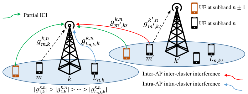
The principal methodology of D-OMA scheme is illustrated in Fig. 1(b) in which the overall system bandwidth ($W$ Hz) is divided into $N$ subbands and each subband is allocated to a sub-set of users (i.e., users in a specific NOMA cluster)¹¹ 1 D-OMA allows different NOMA clusters with adjacent frequency bands to overlap by an amount of $\delta$ percent of their maximum allocated sub-channel. Consequently, the spectral efficiency achieved by massive in-band NOMA cluster is maintained by adding more clusters within the same allocated overall spectrum.. Assume the number of users in subband $n$ at AP $k$ as $L_{n,k}$, and $\mathscr{U}_{k}=\{1,2,...,U_{k}\}$ denotes the set of users in the coverage area of AP $k$. Thus, we have $\sum_{n=1}^{N}L_{n,k}=U_{k}$. We indicate the set of subbands by $\mathscr{N}$ and the set of all APs by $\mathscr{K}$.

In D-OMA method, an additional interference signal named as partial inter-cluster interference (ICI) from the adjacent sub-channels incur. This interference will be observed from users in the same AP as well as other APs. The adjacent subbands are interleaved from the right- and left-side by amount of $\text{B}\times\delta_{n,k}^{r}$ Hz and $\text{B}\times\delta_{n,k}^{l}$ Hz, respectively, where $0\leq\delta_{n,k}^{r}\leq 1$ and $0\leq\delta_{n,k}^{l}\leq 1$ denote the overlap percentage of subband $n$ for AP $k$, and B is the bandwidth of each subband i.e. $\text{B}=\frac{W}{N}$ (see Fig. 1(b)). Note that when $\delta_{n,k}^{r}=\delta_{n,k}^{l}=1$ the subbands are completely overlapped such that the amount of interference power is maximum. On the other hand, each subband’s effective bandwidth denoted by $\text{B}_{n}=\text{B}(1+\delta_{n,k}^{r}+\delta_{n,k}^{l})$ is expanded three times at the expense of additional ICI. Subsequently, the optimal values of $\delta_{n,k}^{r}$ and $\delta_{n,k}^{l}$ for $\forall n\in\mathscr{N}$ and $\forall k\in\mathscr{K}$ and cluster size should be determined efficiently to enhance the network sum rate (SR). Note that $\delta_{n,k}^{r}=0$ and $\delta_{n,k}^{l}=0$ for $\forall n\in\mathscr{N}$ and $\forall k\in\mathscr{K}$ correspond to the conventional NOMA-OFDM.

Let $p_{m,k}$ denote the transmitted data power from the user equipment (UE) $m$ to the AP $k$. To model the subband allocation, we define the following binary variable

Therefore, the received signal at AP $k$ in subband $n$ will be as given in

where $w^{n}_{k}\sim\mathcal{C}\mathcal{N}(0,\sigma^{2})$ is the additive complex Gaussian white noise for a given bandwidth B, in which the noise power is increased due to subband expansion to $(1+\delta_{n,k}^{l}+\delta_{n,k}^{r})\sigma^{2}$, $s_{m,k}$ represents the transmitted symbol from UE $m$ to the AP $k$ with $\mathbb{E}[|s_{m,k}|^{2}]=1$, $\delta_{n,k}^{r}$ and $\delta_{n,k}^{l}$ are the introduced parameters to control the partial ICI at the subband $n$ in AP $k$. It is worth noting that the ICI is caused by using the same subband by other nearby clusters. The users within a certain cluster will suffer from ICI resulting from use of the same subband by other nearby clusters. The size of a NOMA cluster is considered a design parameter to reach trade-offs between different factors, namely, the data-rate necessities of the users; the total power budget per NOMA cluster; the complexity level at the NOMA receivers; and the NOMA user immunity to ICI-based and SIC-based error propagation. On the other hand, SIC allows successive decoding of users’ signals.

It is important to note that there are four types of partial ICI on a given subband $n$ in AP $k$, as illustrated in Fig. 1(b). For instance, the partial ICI on the left-hand side is due to the expansion of subband $n-1$ towards the right-hand side which is controlled by $\delta^{r}_{n-1,k}$ as well as the expansion of subband $n$ to the left-hand side where it is controlled by $\delta^{l}_{n,k}$. The same inference applies to the other two partial ICI signals on the right-hand side of subband $n$.

Note that, $\delta^{r}_{N,k}$ and $\delta^{l}_{1,k}$ do not exist and therefore their value is zero. $g_{m,k^{\prime}}^{k,n}$ indicates the channel power gain between UE $m$ in AP $k^{\prime}$ and AP $k$ at subband $n$ which is denoted as $g_{m,k^{\prime}}^{k,n}=h_{m,k^{\prime}}^{k,n}\sqrt{\beta_{m,k^{\prime}}^{k,n}}$, where $h_{m,k^{\prime}}^{k,n}$ is the small-scale fading coefficient which follows circularly-symmetric zero-mean complex normal distribution with unit variance as $h_{m,k^{\prime}}^{k,n}\sim\mathcal{C}\mathcal{N}(0,1)$ and $\beta_{m,k^{\prime}}^{k,n}$ represents the large-scale fading and path loss. The channel gains are being sorted at APs, i.e., $|g_{1,k}^{k,n}|\geq|g_{2,k}^{k,n}|\geq...\geq|g_{L_{n,k},k}^{k,n}|$, $\forall k\in\mathscr{K}$, $\forall n\in\mathscr{N}$, to perform SIC, in order to extract the desired signal of all UEs. Therefore, the achievable rate of UE $m$ associated with AP $k$ at subband $n$ is given by

where $\text{B}=\frac{W}{N}$, $\text{B}_{n}=\text{B}(1+\delta_{n,k}^{r}+\delta_{n,k}^{l})$, $\tilde{\sigma}^{2}_{n,k}=\sigma^{2}(1+{\delta_{n,k}^{l}}+{\delta_{n,k}^{r}})$, and $\text{I}_{\text{{\color[rgb]{0,0,0}IntraICI}}}^{m,n,k}$, $\text{I}_{\text{{\color[rgb]{0,0,0}InterICI}}}^{m,n,k}$ and $\text{I}_{\text{{\color[rgb]{0,0,0}PartialICI}}}^{m,n,k}$ are defined as

where $\text{I}_{\text{{\color[rgb]{0,0,0}IntraICI}}}^{m,n,k}$ and $\text{I}_{\text{{\color[rgb]{0,0,0}InterICI}}}^{m,n,k}$ are the power of the intra-AP intra-cluster interference and inter-AP inter-cluster interference terms in (1), respectively. Additionally, $\text{I}_{\text{{\color[rgb]{0,0,0}PartialICI}}}^{m,n,k}$ refer to the power of partial ICI components as a function of $\delta_{n,k}^{r}$ and $\delta_{n,k}^{l}$. For simplicity, let us define $\text{I}_{\text{{\color[rgb]{0,0,0}Total}}}^{m,n,k}=\text{I}_{\text{{\color[rgb]{0,0,0}IntraICI}}}^{m,n,k}+\text{I}_{\text{{\color[rgb]{0,0,0}InterICI}}}^{m,n,k}+\text{I}_{\text{{\color[rgb]{0,0,0}PartialICI}}}^{m,n,k}+\tilde{\sigma}^{2}_{n,k}$ as the total interference plus noise power. The total SR of network in bps/Hz is given by $\text{SR}=\displaystyle\sum\limits_{n=1}^{N}\sum\limits_{k=1}^{K}\sum\limits_{m=1}^{U_{k}}\rho_{m,k}^{n}R_{m,k}^{n}$ . It is inferred that by appropriately choosing $\delta_{n,k}^{r}$ and $\delta_{n,k}^{l}$ for $\forall n\in\mathscr{N},\forall k\in\mathscr{K}$, the SR will be increased as well. To the best of our knowledge, the joint optimization of SR and sum power (SP) in terms of finding optimal value of $\boldsymbol{\delta}$, p, and $\boldsymbol{\rho}$ have not been investigated before where we will discuss it in the next subsequent sections. Note that $\boldsymbol{\rho}$, p and $\boldsymbol{\delta}$ are the vector representation of the variables $p_{k,m}$ for $\forall(m,k)\in\mathscr{U}_{k}\times\mathscr{K}$ and $\rho_{m,k}^{n}$, $\forall(m,k,n)\in\mathscr{U}_{k}\times\mathscr{K}\times\mathscr{N}$ and $\delta_{n,k}^{r}$ and $\delta_{n,k}^{l}$ for $\forall(n,k)\in\mathscr{N}$\$N\times\mathscr{K}$, respectively.

Our aim is to optimize the total energy efficiency (EE) which is $\text{EE}=\frac{\text{SR}}{\text{SP}+\text{CP}}$ where $\text{CP}=\sum\limits_{k=1}^{K}\sum\limits_{m=1}^{U_{k}}p^{\text{circuit}}_{m,k}$ denotes the total circuit power consumption with $p^{\text{circuit}}_{m,k}$ for UE $m$ in AP $k$ and $\text{SP}=\sum\limits_{k=1}^{K}\sum\limits_{m=1}^{U_{k}}p_{m,k}$ is the total transmitted data power where $p_{m,k}$ is the transmission power for UE $m$ in AP $k$. It can be easily proved that a problem with the objective of maximizing EE (which is a ratio of total rate to the power consumption) is equivalent to a multi-objective optimization which the objectives are maximizing total rate (the nominator of the EE) and minimizing total power consumption (the denominator of the EE) [12]. Therefore, invoking this property, we formulate a multi-objective optimization problem in the next section.

In this section, we formulate an optimization framework where the objective is to jointly maximize the SR and minimize the total transmitted data power, i.e. SP. The problem formulation is described as follows

where C1 denotes the QoS constraint guaranteeing minimum rate of each user, C2 and C3 are the amount of allowed inter-cluster partial ICI overlapping percentage. The constraint C4 shows that the total number of users in subband $n$ at AP $k$ is $L_{n,k}$ and C5 states that each UE must be allocated to only one subband, C6 is the maximum transmission power constraint for UE $m$. Problem P1 is a type of mixed integer nonlinear and non-convex optimization which is intractable to solve. In order to find the Pareto-optimal solutions for P1, we inspire the Tchebycheff approach [13, 14] which is investigated in the next section comprehensively.

Inspired from weighted max-min formulation for multi-objective optimizations, to convert P1 into a single objective optimization problem we employ Tchebycheff method as it provides complete Pareto-optimal solutions [14]. Henceforth, by applying this method, the multi-objective optimization problem P1 is be transformed as follows:

where $\lambda$ is an auxiliary parameter, $\omega$ is the non-negative weight typically set by a decision maker, and $U_{1}(\boldsymbol{\rho},\textbf{p},\boldsymbol{\delta})=\text{SR}$ where SR is the sum-rate, $U_{2}(\boldsymbol{\rho},\textbf{p},\boldsymbol{\delta})=\text{SP}$ in which SP is the sum-power defined earlier. Furthermore, $U_{i}^{*}$ is the utopia point [14], for $i\in\{1,2\}$ obtained by solving the single-objective problems.

The problem P2 is still non-convex due to binary constraint C7 and non-convex constraint C1. To address this issue, first, we relax the binary constraint C7 then, add a regulation term; next, we combine $p_{m,k}$ and $\rho_{m,k}^{n}$ and introduce new constraint $\tilde{p}_{m,k}^{n}\leq\rho_{m,k}^{n}P^{\text{max}}_{m}$ to be replaced with C6, where it is equal to zero when $\rho_{m,k}^{n}=0$. Therefore, the problem formulation will be

where a regulation term is added to the objective function with parameter $\alpha\gg 1$ that forces the relaxed variables $\rho_{m,k}^{n}$ to be approximately close to either zero or one. For a sufficiently large value of $\alpha$, optimization problem P3 is equivalent to P2 as both problems attain the same optimal values [13]. In other words, the parameter $\alpha$ controls the importance of the regulation term penalty in the objective function, however its value during the simulations shall be chosen properly, since for an exceedingly large $\alpha$, the regulation term would dominate the objective function. Note that $\tilde{\textbf{p}}$ is the vector representation of the new variables $\tilde{p}_{m,k}^{n}$ for $\forall(m,k,n)\in\mathscr{U}_{k}\times\mathscr{K}\times\mathscr{N}$.

In this section, our aim is to convert problem P3 into the caconical form of the monotonic optimization framework [15, 16, 17]. It is observed that the objective and the constraints in P3 are not strictly increasing, however they can be written in terms of difference of increasing functions (DIF). Thus, the following theorem is expressed for optimization problems incorporating DIFs.

Because the the objective and the constraints in P3 do not explicitly indicate monotonicity, our aim is to reformulate P3 to explore some hidden monotonicity. To do so, we first define the following functions

where we observe that $q_{0}^{\pm}(.),q_{1}^{\pm}(.),q_{2}^{\pm}(.),q_{3}^{\pm}(.),q_{4}^{\pm}(.)$ are increasing functions. Now, the constraints can be written in the form of difference of increasing functions. To do so, we define $\tilde{\textbf{p}}_{\text{max}}$ as the tensor containing maximum transmit powers (i.e. $P_{m}^{\text{max}}$), $\boldsymbol{\rho}_{\text{max}}=\textbf{1}$ for $\forall k\in\mathscr{K},m\in\mathscr{U}_{k}$ and $\forall n\in\mathscr{N}$ and $\boldsymbol{\delta}_{\text{max}}=\textbf{1},\forall k\in\mathscr{K},n\in\mathscr{N}$; moreover we set $\lambda_{\text{max}}=\Lambda$. It can be inferred that the problem P3 is an optimization problem where DIFs are used in the objective as well as constraints. Thus, we can convert the problem into an MO by employing Theorem 1. In order to proceed, we define the auxiliary variables $t=q_{0}^{-}(\boldsymbol{\rho}_{\text{max}},\Lambda)-q_{0}^{-}(\boldsymbol{\rho},\lambda)$, $w=q^{-}_{1}(\tilde{\textbf{p}}_{\text{max}},\boldsymbol{\delta}_{\text{max}})-q^{-}_{1}(\tilde{\textbf{p}},\boldsymbol{\delta})$, $l=q^{-}_{2}(\tilde{\textbf{p}}_{\text{max}}$, $\boldsymbol{\delta}_{\text{max}})-q^{-}_{2}(\tilde{\textbf{p}},\boldsymbol{\delta})$, $u=q_{3}^{-}(\tilde{\textbf{\text{p}}}_{\text{max}})-q_{3}^{-}(\tilde{\textbf{\text{p}}})$, $v=q_{4}^{-}(\tilde{\textbf{\text{p}}}_{\text{max}})-q_{4}^{-}(\tilde{\textbf{\text{p}}})$. Then, the problem P3 will be transformed into

where N1–N10 and C2–C5 and $\tilde{\text{C}}$7 are the constraints that build normal set denoted by $\boldsymbol{\Xi}$ and Co-N1–Co-N4 indicate the constraints constructing a co-normal set shown as $\boldsymbol{\Xi}_{c}$. Therefore, P4 is a monotonic optimization in standard canonical form [15]. Henceforth, the optimal solution of P4 lies on the boundary of the feasible set which is defined as $\boldsymbol{\Xi}\cap\boldsymbol{\Xi}_{c}$. A well-known method to solve MO problems is polyblock algorithm [15, 16, 17] in which searches the upper boundary vertex set (edges of the feasible region). The main advantage of employing polyblock algorithm is that the feasible search set is reduced to look up in the boundaries, whereas in the other methods, usually the whole feasible region is exhaustively searched which is intractable and not practical in most cases.

The computational complexity of the polyblock algorithm is severely based on the form of the functions providing number of variables and the normal, co-normal sets. Note that, the size of the vertex set can grow exponentially over iterations, however, some of the vertices are not needed in the computation, and therefore can be safely discarded that accelerate the algorithm speed. Assuming the offered algorithm includes following steps starting from a hyper-rectangle that encloses $\boldsymbol{\Xi}\cap\boldsymbol{\Xi}_{c}$: In the first step, we obtain the best vertex which its projection belongs to the normal set. Next, we obtain the projection of selected vertex on the normal set by using bisection algorithm. The new vertex set is found based on the projection of the vertex on the normal set upperboundary. Then, the improper vertexes that do not satisfy the co-normal constraints are removed. The algorithm continues until a convergence criteria and the best candidate vertex point is reported. While assuming that the dimensions of the optimization problem is $M_{1}$, the number of iterations in overall polyblock algorithm to converge is $M_{2}$ and the number of iteration in bisection algorithm for the projection of each vertex is $M_{3}$. Then, the complexity order is expressed as $\mathcal{O}\left(M_{2}(M_{2}\times M_{1}+M_{3})\right)$.

References

- [1] Y. Al-Eryani and E. Hossain, “The D-OMA method for massive multiple access in 6G: Performance, security, and challenges,” IEEE Veh. Technol. Mag., vol. 14, no. 3, pp. 92–99, Sep. 2019.
- [2] K. David and H. Berndt, “6G vision and requirements: Is there any need for beyond 5G?” IEEE Veh. Technol. Mag., vol. 13, no. 3, pp. 72–80, Sep. 2018.
- [3] Y. Al-Eryani and E. Hossain, “Delta-OMA (D-OMA): A new method for massive multiple access in 6G,” arXiv preprint arXiv:1901.07100, 2019.
- [4] M. S. Ali, H. Tabassum, and E. Hossain, “Dynamic user clustering and power allocation for uplink and downlink non-orthogonal multiple access (NOMA) systems,” IEEE access, vol. 4, pp. 6325–6343, 2016.
- [5] M. Zeng, A. Yadav et al., “Energy-efficient joint user-RB association and power allocation for uplink hybrid NOMA-OMA,” IEEE Internet Things J., vol. 6, no. 3, pp. 5119–5131, Jun 2019.
- [6] J. Shi, W. Yu et al., “Energy efficient resource allocation in hybrid non-orthogonal multiple access systems,” IEEE Trans. Commun., vol. 67, no. 5, pp. 3496–3511, May 2019.
- [7] Y. Sun, D. W. K. Ng et al., “Optimal joint power and subcarrier allocation for full-duplex multicarrier non-orthogonal multiple access systems,” IEEE Trans. Commun., vol. 65, no. 3, pp. 1077–1091, 2017.
- [8] Z. Wei, L. Yang et al., “On the performance gain of NOMA over OMA in uplink communication systems,” IEEE Trans. Commun., vol. 68, no. 1, pp. 536–568, 2020.
- [9] B. Kim, Y. Park, and D. Hong, “Partial non-orthogonal multiple access (P-NOMA),” IEEE Wireless Commun. Lett., vol. 8, no. 5, pp. 1377–1380, Oct. 2019.
- [10] K. S. Ali, E. Hossain, and M. J. Hossain, “Partial non-orthogonal multiple access (NOMA) in downlink poisson networks,” IEEE Trans. Wireless Commun., vol. 19, no. 11, pp. 7637–7652, 2020.
- [11] H. Tabassum, M. S. Ali et al., “Non-orthogonal multiple access (NOMA) in cellular uplink and downlink: challenges and enabling techniques,” Aug. 2016. [Online]. Available: http://arxiv.org/abs/1608.05783
- [12] S. Zarandi, A. Khalili et al., “Multi-objective energy efficient resource allocation and user association for in-band full duplex small-cells,” IEEE Trans. Green Commun. Netw., vol. 4, no. 4, pp. 1048–1060, 2020.
- [13] A. Khalili, M. Robat Mili et al., “Antenna selection strategy for energy efficiency maximization in uplink OFDMA networks: A multi-objective approach,” IEEE Trans. Wirel. Commun., vol. 19, no. 1, pp. 595–609, Jan. 2020.
- [14] R. T. Marler and J. S. Arora, “Survey of multi-objective optimization methods for engineering,” Struct. Multidiscip. Optim., vol. 26, no. 6, pp. 369–395, Apr. 2004.
- [15] H. Tuy, “Monotonic optimization: Problems and solution approaches,” SIAM J. Optim., vol. 11, no. 2, pp. 464–494, Jul. 2000.
- [16] H. Tuy, F. Al-Khayyal, and P. T. Thach, Monotonic optimization: branch and cut methods. Boston, MA: Springer US, 2005, pp. 39–78.
- [17] A. Zappone, E. Björnson et al., “Globally optimal energy-efficient power control and receiver design in wireless networks,” IEEE Trans. Signal Process., vol. 65, no. 11, pp. 2844–2859, Jun. 2017.