跳到论文正文
W Papers独立论文阅读器 arXiv:2102.13270 论文正文 计算阅读时间 · 0%
引用这篇论文根据当前论文元数据生成,正式投稿前建议核对。


License: arXiv.org perpetual non-exclusive license
arXiv:2102.13270v3 [cs.IT] 04 Mar 2021

Single-angle Radon samples based reconstruction of functions in refinable shift-invariant spaceThanks: Youfa Li is partially supported by Natural Science Foundation of China (Nos: 61961003, 61561006, 11501132), Natural Science Foundation of Guangxi (Nos: 2018JJA110110, 2016GXNSFAA380049) and the talent project of Education Department of Guangxi Government for Young-Middle-Aged backbone teachers.

Youfa Li Address: College of Mathematics and Information Science
Guangxi University, Nanning, China
Email address: youfalee@hotmail.com
, Shengli Fan Address: CREOL College of Optics & Photonics
University of Central Florida, Orlando, FL 32816
Email address: shengli.fan@knights.ucf.edu
and Yanfeng Huang Address: College of Mathematics and Information Science
Guangxi University, Nanning, China
Email address: hyfbqy@163.com
Date: August 11, 2026
Abstract.

The traditional approaches to computerized tomography (CT) depend on the samples of Radon transform at multiple angles. In optics, the real time imaging requires the reconstruction of an object by the samples of Radon transform at a single angle (SA). Driven by this and motivated by the connection between Bin Han’s construction of wavelet frames (e.g [13]) and Radon transform, in refinable shift-invariant spaces (SISs) we investigate the SA-Radon sample based reconstruction problem. We have two main theorems. The fist main theorem states that, any compactly supported function in a SIS generated by a general refinable function can be determined by its Radon samples at an appropriate angle. Motivated by the extensive application of positive definite (PD) functions to interpolation of scattered data, we also investigate the SA reconstruction problem in a class of (refinable) box-spline generated SISs. Thanks to the PD property of the Radon transform of such spline, our second main theorem states that, the reconstruction of compactly supported functions in these spline generated SISs can be achieved by the samples of Radon transform at almost every angle. Numerical simulation is conducted to check the result.

Key words and phrases: 
computerized tomography, single-angle Radon sample, refinable shift-invariant spaces, box-spline, positive definite function
2010 Mathematics Subject Classification
Primary 42C40; 65T60; 94A20

1. Introduction

1.1. CT and Radon transform

We start with the X-ray computerized tomography (CT) on ℝ2\mathbb{R}^{2}. Its core mathematics includes the Radon transform and its inversion. For a function f∈L2​(ℝ2)f\in L^{2}(\mathbb{R}^{2}), the Radon transform, w.r.t a fixed angle θ∈[0,2​π)\theta\in[0,2\pi), at t∈ℝt\in\mathbb{R} is defined as the integral of ff along the line (x,y)=t⁡(cos⁡θ,sin⁡θ)+s⁡(−sin⁡θ,cos⁡θ):(x,y)=t(\cos\theta,\sin\theta)+s(-\sin\theta,\cos\theta):

(1.1) ∫−∞∞f⁡(t​cos⁡θ−s​sin⁡θ,t​sin⁡θ+s​cos⁡θ)​𝑑s.\displaystyle\int^{\infty}_{-\infty}f(t\cos\theta-s\sin\theta,t\sin\theta+s\cos\theta)ds.

Denote P=[cos⁡θ,sin⁡θ]P=[\cos\theta,\sin\theta]. For simplicity, following B. Han [13] the Radon transform in (1.1) is denoted as

P​f​(t)=∫−∞∞f⁡(t​cos⁡θ−s​sin⁡θ,t​sin⁡θ+s​cos⁡θ)​𝑑s.Pf(t)=\int^{\infty}_{-\infty}f(t\cos\theta-s\sin\theta,t\sin\theta+s\cos\theta)ds.

The Fourier transform of P​fPf can be expressed as

(1.2) P​f^​(ξ)=f^​(PT​ξ)=f^​(ξ​cos⁡θ,ξ​sin⁡θ),ξ∈ℝ,\displaystyle\widehat{Pf}(\xi)=\widehat{f}(P^{T}\xi)=\widehat{f}(\xi\cos\theta,\xi\sin\theta),\quad\xi\in\mathbb{R},

where for any function g∈Lp​(ℝD)g\in L^{p}(\mathbb{R}^{D}) its Fourier transform at γ∈ℝD\gamma\in\mathbb{R}^{D} is defined as g^(γ):=∫ℝDg(x)e−ix⋅γdx\widehat{g}(\gamma):=\int_{\mathbb{R}^{D}}g(x)e^{-\textbf{i}x\cdot\gamma}dx. It follows from (1.2) that P​f^\widehat{Pf} is essentially the projection of f^\widehat{f} onto the subspace (slice) {PT​ξ:ξ∈ℝ}\{P^{T}\xi:\xi\in\mathbb{R}\}. Correspondingly, from now on PP is called the projection vector. On the other hand, ff can be reconstructed via the so called inverse Radon transform (c.f.[29]):

(1.3) f⁡(x,y)=14​π2​∫02​π∫0∞f^​(PT​ξ)​ei​ξ​(x​cos⁡θ+y​sin⁡θ)​ξ​𝑑ξ​𝑑θ,\displaystyle f(x,y)=\frac{1}{4\pi^{2}}\int^{2\pi}_{0}\int^{\infty}_{0}\widehat{f}(P^{T}\xi)e^{\textbf{i}\xi(x\cos\theta+y\sin\theta)}\xi d\xi d\theta,

with P=[cos⁡θ,sin⁡θ].P=[\cos\theta,\sin\theta].

1.2. Traditional approaches conducted by Radon transforms at multiple angles

Theoretically, (1.3) implies that the reconstruction of ff requires the projections f^​(PT​ξ)\widehat{f}(P^{T}\xi) for all angle θ\theta. In practice, however, what we can observe are the samples of limited projections. Therefore, the essential problem of CT (also referred to as the limited angle problem (LAP)) is to construct the approximation to ff by the samples of finitely many projections. The most classical approximation is the filtered backprojection (FBP) (c.f. [19, 10]) derived from (1.3). In principle, FBP requires ff to be bandlimited and needs the Fourier samples. If FBP is applied to non-bandlimited functions, then the low-pass filtering (to cut off the high-frequency component) and linear interpolation are commonly necessary. They may introduce serious errors (c.f. [35, 30]).

Some recent alternatives to FBP have been introduced (e.g. [8, 21, 26, 28, 35]). Unlike FBP, they are conducted by the samples of Radon transforms. For example, based on the orthogonal polynomial system, Xu [35] established the approach to CT. Entezari, Nilchian and Unser [8] and McCann and Unser [28] established a spline-based reconstruction. Note that the samples required for the above approaches are derived from Radon transforms at multiple angles.

Contrary to the traditional approaches requiring multiple angles, our purpose is to reconstruct a function by the samples of its Radon transform at a single angle (SA). In what follows, we introduce the requirement for such a SA-based approach in optical imaging.

1.3. SA-based reconstruction is required for real time imaging

Optical imaging has been widely used in observing biological objects, such as blood cells (thin objects) and bones (thick objects). The thin objects are commonly imaged directly by refractive-index distributions, which is achieved by holographic tomography (HT) ([22]). However, for imaging thick objects, CT is usually employed.

CT commonly requires samples (measurements) of the light fields penetrating through the object from different angles (views). To do so, the object needs to be rotated by a rotation motor ([36]) or the illumination needs to be scanned by a beam steering device, which not only causes instability for the imaging system, but makes the system bulky ([3, 27]). More importantly, limited by the time of recording fields, rotating objects or scanning illuminations becomes not suitable for real-time imaging, especially for observing fast dynamic events ([27]). Now a natural imaging problem is:

(1.4) can CT be achieved by the samples of SA-Radon transform?

Most recently, R. Horisaki, K. Fujii, and J. Tanida [27] established a SA method for HT by inserting a diffuser. However, to our best of knowledge, (1.4) (the SA problem for CT) is very challenging and remains less explored. The purpose of this paper is to investigate it from the mathematical perspective. In what follows, we organize the problem in the present paper.

1.4. The mathematical problem of SA-based reconstruction in refinable SISs

Recall that the refinable shift-invariant space (SIS) is a type of function space that is widely used in signal processing and time-frequency analysis (e.g. [1, 9, 31, 32, 33]). On the other hand, motivated by the connection between Bin Han’s construction of wavelet frames (c.f. [13, 14, 15, 17] and to be introduced in subsection 2.1) and Radon transform (1.2), we will investigate the following problem:

Q:Can one reconstruct a function in a refinable SIS by its SA-Randon (transform)samples​?\displaystyle\begin{array}[]{llll}\hbox{{Q}}:\hbox{Can one reconstruct a function in a refinable SIS by its SA-Randon (transform)}\\ \quad\quad\hbox{samples}?\end{array}

As the problem (1.4) in optics, the above problem is still less explored in mathematics. It might be ”stereotyped” by the inverse Radon transform (1.3) which requires the Fourier samples of Radon transform at multiple angles.

1.5. Our contributions

Our main results are organized in Theorems 3.1 and 4.3. In Theorem 3.1 we prove that, any compactly supported function from a general refinable SIS can be exactly reconstructed by its Radon samples at the appropriate angle. For a class of refinable box-splines, we prove that their Radon transforms at any angle are positive definite (PD). And Theorem 4.3 states that for almost every angle θ∈[0,2​π)\theta\in[0,2\pi), any compactly supported function in such box-splines generated SISs can be reconstructed by its Radon (transform at angle θ\theta) samples.

2. Preliminary

2.1. Connection between Han’s construction of wavelet frame and Radon transform (1.2)

B. Han et.al [13, 14, 15, 17] and [16, Section 7.1.3] provided the projection method for constructing wavelet frames. Specifically, the wavelet frames {ψ1,…,ψL}⊆L2​(ℝ2)\{\psi^{1},\ldots,\psi^{L}\}\subseteq L^{2}(\mathbb{R}^{2}) are first constructed, then the ones {P~​ψ1,…,P~​ψL}⊆L2​(ℝ)\{\tilde{P}\psi^{1},\ldots,\tilde{P}\psi^{L}\}\subseteq L^{2}(\mathbb{R}) defined by

(2.1) P~​ψl^​(ξ)=ψl^​(P~T​ξ)\displaystyle\widehat{\tilde{P}\psi^{l}}(\xi)=\widehat{\psi^{l}}(\tilde{P}^{T}\xi)

can have desirable properties if choosing an appropriate vector P~∈ℤ1×2\tilde{P}\in\mathbb{Z}^{1\times 2}. Note that both (1.2) and (2.1) take the identical form. Moreover, since P~​ψl^=ψl^​(‖P~‖2​P~T‖P~‖2​ξ)\widehat{\tilde{P}\psi^{l}}=\widehat{\psi^{l}}(\|\tilde{P}\|_{2}\frac{\tilde{P}^{T}}{\|\tilde{P}\|_{2}}\xi) then P~​ψl\tilde{P}\psi^{l} is essentially the composition of Radon transform (projection vector: P~T‖P~‖2\frac{\tilde{P}^{T}}{\|\tilde{P}\|_{2}}) and the dilation operation (dilation factor: ‖P~‖2−1\|\tilde{P}\|^{-1}_{2}).

2.2. On the support of P~​f\tilde{P}f defined via (2.1)

For a function f∈L1​(ℝ2)f\in L^{1}(\mathbb{R}^{2}) and a vector P~∈ℝ1×2\tilde{P}\in\mathbb{R}^{1\times 2}, motivated by [13, 16] we next address the relationship between P~​f\tilde{P}f and ff in the spatial domain. Denote the singular value decomposition (SVD) of P~\tilde{P} by P~=Σ​VT\tilde{P}=\Sigma V^{T}, where VV is a 2×22\times 2 real-valued unitary matrix, and Σ=[σ,0]\Sigma=[\sigma,0] with σ=‖P‖2\sigma=\|P\|_{2}. Now it follows from [13, 16] that P~​f=Σ⁡(VT​f),\tilde{P}f=\Sigma(V^{T}f), where VT​f​(x)=f⁡((VT)−1​x)V^{T}f(x)=f((V^{T})^{-1}x) with x=(x1,x2)T∈ℝ2x=(x_{1},x_{2})^{T}\in\mathbb{R}^{2}, and for any gg on ℝ2\mathbb{R}^{2} the function Σ​g\Sigma g is defined by

(2.2) Σ​g​(x1)=σ−1​∫ℝg⁡(σ−1​x1,x2)​d​x2.\displaystyle\Sigma g(x_{1})=\sigma^{-1}\int_{\mathbb{R}}g(\sigma^{-1}x_{1},x_{2})dx_{2}.

It is easy to check that if f∈L1​(ℝ2)f\in L^{1}(\mathbb{R}^{2}) then P~​f∈L1​(ℝ)\tilde{P}f\in L^{1}(\mathbb{R}). Moreover, the following lemma states that if f∈L2​(ℝ2)f\in L^{2}(\mathbb{R}^{2}) is compactly supported, then P~​f\tilde{P}f still lies in L2​(ℝ)L^{2}(\mathbb{R}) and is also compactly supported.

Lemma 2.1.

Suppose that f∈L2​(ℝ2)f\in L^{2}(\mathbb{R}^{2}) is compactly supported on [a1,b1]×[a2,b2][a_{1},b_{1}]\times[a_{2},b_{2}]. For 0≠P~∈ℝ1×20\neq\tilde{P}\in\mathbb{R}^{1\times 2}, define P~​f\tilde{P}f via (2.1). Then

(2.3) supp(P~f)⊆[−2∥P~∥2max{|bi|,|ai|:i=1,2},2∥P~∥2max{|bi|,|ai|:i=1,2}],\displaystyle\hbox{supp}(\tilde{P}f)\subseteq[-\sqrt{2}\|\tilde{P}\|_{2}\max\{|b_{i}|,|a_{i}|:i=1,2\},\sqrt{2}\|\tilde{P}\|_{2}\max\{|b_{i}|,|a_{i}|:i=1,2\}],

and P~​f∈L2​(ℝ)\tilde{P}f\in L^{2}(\mathbb{R}).

Proof.

Denote VT​fV^{T}f by g.g. Then for any x1∈ℝ,x_{1}\in\mathbb{R},

P~​f​(x1)=Σ​g​(x1)=σ−1​∫ℝg⁡(σ−1​x1,x2)​d​x2=σ−1​∫ℝ[VT​f]​(σ−1​x1,x2)​d​x2=σ−1​∫ℝf⁡(V​(σ−1​x1,x2)T)​d​x2,\displaystyle\begin{array}[]{llll}\tilde{P}f(x_{1})&=\displaystyle\Sigma g(x_{1})\\ &\displaystyle=\sigma^{-1}\int_{\mathbb{R}}g(\sigma^{-1}x_{1},x_{2})dx_{2}\\ &\displaystyle=\sigma^{-1}\int_{\mathbb{R}}[V^{T}f](\sigma^{-1}x_{1},x_{2})dx_{2}\\ &\displaystyle=\sigma^{-1}\int_{\mathbb{R}}f(V(\sigma^{-1}x_{1},x_{2})^{T})dx_{2},\end{array}

where σ=‖P~‖2\sigma=\|\tilde{P}\|_{2}, the second and last equalities are derived from (2.2) and VV being a real-valued unitary matrix. It follows from supp​(f)⊆[a1,b1]×[a2,b2]\hbox{supp}(f)\subseteq[a_{1},b_{1}]\times[a_{2},b_{2}] that for any x∈supp​(f)x\in\hbox{supp}(f), we have ∥x∥2≤2max{|bi|,|ai|:i=1,2}\|x\|_{2}\leq\sqrt{2}\max\{|b_{i}|,|a_{i}|:i=1,2\}. Now by (2.2) and VV being a unitary matrix it is easy to check that (2.3) holds. Define G⁡(x1,x2):=f⁡(V​(x1,x2)T)G(x_{1},x_{2}):=f(V(x_{1},x_{2})^{T}). For any (x1,x2)T∈supp​(G)(x_{1},x_{2})^{T}\in\hbox{supp}(G), through the similar analysis as above we have

(2.8) |x2|≤2max{|bi|,|ai|:i=1,2}.\displaystyle|x_{2}|\leq\sqrt{2}\max\{|b_{i}|,|a_{i}|:i=1,2\}.

Moreover,

‖P~​f‖L22=‖Σ⁡(VT​f)‖L22=1σ2​∫ℝ|∫ℝ[VT​f]​(σ−1​x1,x2)​d​x2|2​d​x1≤2max{|bi|,|ai|:i=1,2}σ2∫ℝ∫ℝ|[VTf](σ−1x1,x2)|2dx2dx1≤2max{|bi|,|ai|:i=1,2}σ∥f∥L22<∞,\displaystyle\begin{array}[]{llll}\|\tilde{P}f\|_{L^{2}}^{2}&=\|\Sigma(V^{T}f)\|_{L^{2}}^{2}\\ &\displaystyle=\frac{1}{\sigma^{2}}\int_{\mathbb{R}}\big|\int_{\mathbb{R}}[V^{T}f](\sigma^{-1}x_{1},x_{2})dx_{2}\big|^{2}dx_{1}\\ &\displaystyle\leq\frac{\sqrt{2}\max\{|b_{i}|,|a_{i}|:i=1,2\}}{\sigma^{2}}\int_{\mathbb{R}}\int_{\mathbb{R}}|[V^{T}f](\sigma^{-1}x_{1},x_{2})|^{2}dx_{2}dx_{1}\\ &\displaystyle\leq\frac{\sqrt{2}\max\{|b_{i}|,|a_{i}|:i=1,2\}}{\sigma}\|f\|_{L^{2}}^{2}<\infty,\end{array}

where the first inequality is derived from (2.8) and the Cauchy-Swart inequality. The proof is concluded. ∎

2.3. (Quasi) shift-invariant space

The space of square summable sequences on ℤD\mathbb{Z}^{D} is defined as ℓ2​(ℤD):={{ck}k∈ℤD:‖{ck}k∈ℤD‖ℓ2=[∑k∈ℤD|ck|2]1/2<∞}\ell^{2}(\mathbb{Z}^{D}):=\big\{\{c_{k}\}_{k\in\mathbb{Z}^{D}}:\|\{c_{k}\}_{k\in\mathbb{Z}^{D}}\|_{\ell^{2}}=[\sum_{k\in\mathbb{Z}^{D}}|c_{k}|^{2}]^{1/2}<\infty\big\}. For a generator ϕ∈L2​(ℝD)\phi\in L^{2}(\mathbb{R}^{D}) with D≥1D\geq 1, the associated shift-invariant space (SIS) V⁡(ϕ,ℤD)V(\phi,\mathbb{Z}^{D}) is defined as

(2.13) V(ϕ,ℤD)={∑k∈ℤDckϕ(⋅−k):{ck}k∈ℤD∈ℓ2(ℤD)}.\displaystyle V(\phi,\mathbb{Z}^{D})=\Big\{\sum_{k\in\mathbb{Z}^{D}}c_{k}\phi(\cdot-k):\{c_{k}\}_{k\in\mathbb{Z}^{D}}\in\ell^{2}(\mathbb{Z}^{D})\Big\}.

For the stable recovery of functions in V⁡(ϕ,ℤD)V(\phi,\mathbb{Z}^{D}), it is commonly required that {ϕ(⋅−k):k∈ℤD}\big\{\phi(\cdot-k):k\in\mathbb{Z}^{D}\big\} is a Riesz basis for V⁡(ϕ,ℤD)V(\phi,\mathbb{Z}^{D}) (c.f. [1, 2, 23]), namely, there exist 0<C1≤C2<∞0<C_{1}\leq C_{2}<\infty such that

(2.14) C1∥{ck}k∈ℤD∥ℓ22≤∥∑k∈ℤDckϕ(⋅−k)∥L22≤C2∥{ck}k∈ℤD∥ℓ22.\displaystyle C_{1}\|\{c_{k}\}_{k\in\mathbb{Z}^{D}}\|^{2}_{\ell^{2}}\leq\big\|\sum_{k\in\mathbb{Z}^{D}}c_{k}\phi(\cdot-k)\big\|^{2}_{L^{2}}\leq C_{2}\|\{c_{k}\}_{k\in\mathbb{Z}^{D}}\|^{2}_{\ell^{2}}.

Here C1C_{1} and C2C_{2} are referred to as the Riesz lower and upper bounds of {ϕ(⋅−k):k∈ℤD}\{\phi(\cdot-k):k\in\mathbb{Z}^{D}\}. For a generator φ∈L2​(ℝD)\varphi\in L^{2}(\mathbb{R}^{D}) and the shift set 𝒳={xj}j∈ℤD⊆ℝD\mathcal{X}=\{x_{j}\}_{j\in\mathbb{Z}^{D}}\subseteq\mathbb{R}^{D}, the associated quasi shift-invariant space (QSIS) is defined as

(2.15) V(φ,𝒳):={∑k∈ℤDckφ(⋅−xj):{ck}k∈ℤD∈ℓ2(ℤD)}.\displaystyle V(\varphi,\mathcal{X}):=\Big\{\sum_{k\in\mathbb{Z}^{D}}c_{k}\varphi(\cdot-x_{j}):\{c_{k}\}_{k\in\mathbb{Z}^{D}}\in\ell^{2}(\mathbb{Z}^{D})\Big\}.

If 𝒳=ℤ\mathcal{X}=\mathbb{Z} then V⁡(φ,𝒳)V(\varphi,\mathcal{X}) degenerates to be an SIS. As implied in [12], the recovery theory for the QSIS (𝒳≠ℤ\mathcal{X}\neq\mathbb{Z} ) is not the trivial generalization of that for the SIS. For example, the generator for the QSIS needs to be a positive definite function (the definition is postponed to section 4) such that the recovery can be achieved (c.f. [12, section 3.1(A1)]). Readers can refer to [4, 5, 11, 12] for the recent recovery results in QSISs (generated from some interesting generators such as the sinc and Gaussian functions).

2.4. On the Sobolev smoothness of a function

For any ς∈ℝ\varsigma\in\mathbb{R}, the Sobolev space Hς​(ℝD)H^{\varsigma}(\mathbb{R}^{D}) is defined as

Hς​(ℝD):={f:∫ℝD|f^​(ξ)|2​(1+‖ξ‖22)ς​dξ<∞}.\displaystyle\begin{array}[]{lllll}\displaystyle H^{\varsigma}(\mathbb{R}^{D}):=\Big\{f:\int_{\mathbb{R}^{D}}|\widehat{f}(\xi)|^{2}(1+\|\xi\|_{2}^{2})^{\varsigma}d\xi<\infty\Big\}.\end{array}

The deduced norm is defined by

∥f∥Hς​(ℝD):=1(2​π)D/2(∫ℝD|f^(ξ)|2(1+∥ξ∥22)ςdξ)1/2,∀f∈Hς(ℝD).\displaystyle\begin{array}[]{lllll}\displaystyle\|f\|_{H^{\varsigma}(\mathbb{R}^{D})}:=\frac{1}{(2\pi)^{D/2}}\Big(\int_{\mathbb{R}^{D}}|\widehat{f}(\xi)|^{2}(1+\|\xi\|_{2}^{2})^{\varsigma}d\xi\Big)^{1/2},\quad\forall f\in H^{\varsigma}(\mathbb{R}^{D}).\end{array}

And the Sobolev smoothness of ff is defined as ν2​(f):=sup{ς:f∈Hς​(ℝD)}\nu_{2}(f):=\sup\{\varsigma:f\in H^{\varsigma}(\mathbb{R}^{D})\}. For ς>D/2\varsigma>D/2, by [31, Chapter 9.1] or [24, section 1] the functions in Hς​(ℝD)H^{\varsigma}(\mathbb{R}^{D}) are continuous.

3. SA-Radon samples based reconstruction for compactly supported functions in general refinable SISs

Some definitions and denotations are necessary for our discussion. For a SIS V⁡(ϕ,ℤD)V(\phi,\mathbb{Z}^{D}) and a compact set E⊆ℝDE\subseteq\mathbb{R}^{D}, define

VE​(ϕ,ℤD):={f∈V⁡(ϕ,ℤD):supp​(f)⊆E}.V_{E}(\phi,\mathbb{Z}^{D}):=\{f\in V(\phi,\mathbb{Z}^{D}):\hbox{supp}(f)\subseteq E\}.

Denote by ⌊x⌋\lfloor x\rfloor (⌈x⌉\lceil x\rceil) the largest (smallest) number that is not larger (not smaller) than xx. The cardinality of a set GG is denoted by #​G\#G. A function ϕ∈L2​(ℝD)\phi\in L^{2}(\mathbb{R}^{D}) is refinable if ϕ^​(2​ξ)=a^​(ξ)​ϕ^​(ξ)\widehat{\phi}(2\xi)=\widehat{a}(\xi)\widehat{\phi}(\xi) where a^​(ξ)\widehat{a}(\xi) is a 2​π​ℤD2\pi\mathbb{Z}^{D}-periodic trigonometric polynomial (c.f. [6, 16, 25]). In what follows we establish the first main theorem in this paper.

3.1. The first main theorem

The following is the first main result in this paper.

Theorem 3.1.

Suppose that ϕ∈L2​(ℝ2)\phi\in L^{2}(\mathbb{R}^{2}) is refinable and continuous such that supp​(ϕ)⊆[N1,M1]×[N2,M2]\hbox{supp}(\phi)\subseteq[N_{1},M_{1}]\times[N_{2},M_{2}]. Moreover, suppose that the projection vector P∈ℝ1×2P\in\mathbb{R}^{1\times 2} and there exists γ∈ℝ\gamma\in\mathbb{R} such that γ​P∈ℤ1×2\gamma P\in\mathbb{Z}^{1\times 2} and {γ​P​x:x∈ℤ2}=ℤ\{\gamma Px:x\in\mathbb{Z}^{2}\}=\mathbb{Z}. Then for almost all discrete set X⊆(0,1)X\subseteq(0,1) such that 2≤#​X<∞2\leq\#X<\infty, any f∈VE​(ϕ,ℤ2)f\in V_{E}(\phi,\mathbb{Z}^{2}) with E=[a1,b1]×[a2,b2]E=[a_{1},b_{1}]\times[a_{2},b_{2}] can be determined by the samples of its SA-Radon transform P​fPf at

(X/γ+ℤ/γ)⋂[−2max{|Ni|,|Mi|:i=1,2}+Kmin,2max{|Ni|,|Mi|:i=1,2}+Kmax],\displaystyle\begin{array}[]{lllllllll}\big(X/\gamma+\mathbb{Z}/\gamma\big)\\ \bigcap\Big[-\sqrt{2}\max\{|N_{i}|,|M_{i}|:i=1,2\}+K_{\min},\sqrt{2}\max\{|N_{i}|,|M_{i}|:i=1,2\}+K_{\max}\Big],\end{array}

provided that the map PE̊:E̊⟶ℤP_{\mathring{E}}:\mathring{E}\longrightarrow\mathbb{Z} defined by PE̊​(x)=P​xP_{\mathring{E}}(x)=Px is an injection, where

(3.3) E̊={[⌈a1−M1⌉,⌊b1−N1⌋]×[⌈a2−M2⌉,⌊b2−N2⌋]}∩ℤ2,\displaystyle\mathring{E}=\Big\{\Big[\lceil a_{1}-M_{1}\rceil,\lfloor b_{1}-N_{1}\rfloor\Big]\times\Big[\lceil a_{2}-M_{2}\rceil,\lfloor b_{2}-N_{2}\rfloor\Big]\Big\}\cap\mathbb{Z}^{2},

Kmin=min⁡{γ​P​k:k∈E̊}K_{\min}=\min\{\gamma Pk:k\in\mathring{E}\} and Kmax=max⁡{γ​P​k:k∈E̊}K_{\max}=\max\{\gamma Pk:k\in\mathring{E}\}.

Proof.

The proof is given in subsection 3.3. ∎

Remark 3.1.

In Theorem 3.1, we assume that the functions to be reconstructed are compactly supported and their supports are contained in a known rectangle. Such an assumption is reasonable for CT (c.f. [35]).

3.2. Design of feasible projection vector

In Theorem 3.1 the projection vector PP is required to satisfy the following two conditions:

(A1):(A_{1}): the map PE̊:E̊⟶ℤP_{\mathring{E}}:\mathring{E}\longrightarrow\mathbb{Z} defined by PE̊​(x)=P​xP_{\mathring{E}}(x)=Px is injective.

(A2):(A_{2}): there exists 0≠γ∈ℝ0\neq\gamma\in\mathbb{R} such that {γ​P​x:x∈ℤ2}=ℤ.\{\gamma Px:x\in\mathbb{Z}^{2}\}=\mathbb{Z}.

In what follows, we establish a choice of PP such that (A1)(A_{1}) and (A2)(A_{2}) hold.

Proposition 3.2.

Define E̊−:={k−k^:k,k^∈E̊}\mathring{E}^{-}:=\{k-\hat{k}:k,\hat{k}\in\mathring{E}\}. For j=1,2j=1,2, denote E̊j,max−:={|⟨k,ej⟩|:k∈E̊−}\mathring{E}^{-}_{j,\max}:=\{|\langle k,e_{j}\rangle|:k\in\mathring{E}^{-}\}, where ej∈ℝ2e_{j}\in\mathbb{R}^{2} is the jjth unit coordinate vector with the only nonzero entry 11 at the jjth entry. Choose P~=[P~1,P~2]\tilde{P}=[\tilde{P}_{1},\tilde{P}_{2}] recursively by P~1=1\tilde{P}_{1}=1, P~2=E̊1,max−+P~1\tilde{P}_{2}=\mathring{E}^{-}_{1,\max}+\tilde{P}_{1}. Then P=P~‖P~‖2P=\frac{\tilde{P}}{\|\tilde{P}\|_{2}} satisfies (A1)(A_{1}) and (A2).(A_{2}).

Proof.

It is easy to prove that (A1)(A_{1}) holds if and only if ⟨P~,k⟩≠0\langle\tilde{P},k\rangle\neq 0 for any fixed 0≠k=(k1,k2)∈E̊−.\textbf{0}\neq k=(k_{1},k_{2})\in\mathring{E}^{-}. Denote Jk=max⁡{j:kj≠0}J_{k}=\max\{j:k_{j}\neq 0\}. If Jk=1J_{k}=1, then clearly |⟨P~,k⟩|≥1|\langle\tilde{P},k\rangle|\geq 1. If Jk=2J_{k}=2, then

|⟨P~,k⟩|≥|P~2​k2|−|P~1​k1|=|P~2​k2|−|k1|≥|P~2|−|k1|≥|P~2|−E̊1,max−=1.|\langle\tilde{P},k\rangle|\geq|\tilde{P}_{2}k_{2}|-|\tilde{P}_{1}k_{1}|=|\tilde{P}_{2}k_{2}|-|k_{1}|\geq|\tilde{P}_{2}|-|k_{1}|\geq|\tilde{P}_{2}|-\mathring{E}^{-}_{1,\max}=1.

Then (A1)(A_{1}) holds. Since ⟨P~,e1⟩=P~1=1\langle\tilde{P},e_{1}\rangle=\tilde{P}_{1}=1 then (A2)(A_{2}) holds with γ=‖P~‖2\gamma=\|\tilde{P}\|_{2}. ∎

3.3. Proof of Theorem 3.1

3.3.1. Two lemmas

In the following lemma, we establish a necessary and sufficient condition on the generator Radon transform P​ϕP\phi, such that any compactly supported f∈V⁡(ϕ,ℤ2)f\in V(\phi,\mathbb{Z}^{2}) can be determined by its SA-Radon transform P​f.Pf.

Lemma 3.3.

Suppose that ϕ∈L2​(ℝ2)\phi\in L^{2}(\mathbb{R}^{2}) is refinable such that supp​(ϕ)⊆[N1,M1]×[N2,M2]\hbox{supp}(\phi)\subseteq[N_{1},M_{1}]\times[N_{2},M_{2}]. Then any f∈VE​(ϕ,ℤ2)f\in V_{E}(\phi,\mathbb{Z}^{2}) can be determined by its Radon transform P​fPf if and only if {Pϕ(⋅−Pk):k∈E̊}\{P\phi(\cdot-Pk):k\in\mathring{E}\} is a basis for span{Pϕ(⋅−Pk):k∈E̊}\hbox{span}\{P\phi(\cdot-Pk):k\in\mathring{E}\}, where E=[a1,b1]×[a2,b2]E=[a_{1},b_{1}]\times[a_{2},b_{2}] and

(3.4) E̊={[⌈a1−M1⌉,⌊b1−N1⌋]×[⌈a2−M2⌉,⌊b2−N2⌋]}∩ℤ2.\displaystyle\mathring{E}=\Big\{\Big[\lceil a_{1}-M_{1}\rceil,\lfloor b_{1}-N_{1}\rfloor\Big]\times\Big[\lceil a_{2}-M_{2}\rceil,\lfloor b_{2}-N_{2}\rfloor\Big]\Big\}\cap\mathbb{Z}^{2}.
Proof.

Necessity: For f∈VE​(ϕ,ℤ2)f\in V_{E}(\phi,\mathbb{Z}^{2}), it follows from supp​(f)⊆E\hbox{supp}(f)\subseteq E that

(3.5) f=∑k1=⌈a1−M1⌉⌊b1−N1⌋∑k2=⌈a2−M2⌉⌊b2−N2⌋ck1,k2ϕ(⋅−k1,⋅−k2).\displaystyle f=\sum^{\lfloor b_{1}-N_{1}\rfloor}_{k_{1}=\lceil a_{1}-M_{1}\rceil}\sum^{\lfloor b_{2}-N_{2}\rfloor}_{k_{2}=\lceil a_{2}-M_{2}\rceil}c_{k_{1},k_{2}}\phi(\cdot-k_{1},\cdot-k_{2}).

Then for any ξ∈ℝ\xi\in\mathbb{R}, we have

P​f^​(ξ)=f^​(PT​ξ)=∑⌊b1−N1⌋k1=⌈a1−M1⌉∑⌊b2−N2⌋k2=⌈a2−M2⌉ck1,k2e−ik⋅PTξϕ^(PTξ)=∑⌊b1−N1⌋k1=⌈a1−M1⌉∑⌊b2−N2⌋k2=⌈a2−M2⌉ck1,k2e−iPk⋅ξP​ϕ^(ξ),\displaystyle\begin{array}[]{llll}\widehat{Pf}(\xi)&=\widehat{f}(P^{T}\xi)&=\displaystyle\sum^{\lfloor b_{1}-N_{1}\rfloor}_{k_{1}=\lceil a_{1}-M_{1}\rceil}\sum^{\lfloor b_{2}-N_{2}\rfloor}_{k_{2}=\lceil a_{2}-M_{2}\rceil}c_{k_{1},k_{2}}e^{-\textbf{i}k\cdot P^{T}\xi}\widehat{\phi}(P^{T}\xi)\\ &&=\displaystyle\sum^{\lfloor b_{1}-N_{1}\rfloor}_{k_{1}=\lceil a_{1}-M_{1}\rceil}\sum^{\lfloor b_{2}-N_{2}\rfloor}_{k_{2}=\lceil a_{2}-M_{2}\rceil}c_{k_{1},k_{2}}e^{-\textbf{i}Pk\cdot\xi}\widehat{P\phi}(\xi),\end{array}

where k=(k1,k2)Tk=(k_{1},k_{2})^{T}. That is,

(3.8) Pf=∑k1=⌈a1−M1⌉⌊b1−N1⌋∑k2=⌈a2−M2⌉⌊b2−N2⌋ck1,k2Pϕ(⋅−Pk)∈span{Pϕ(⋅−Pk):k∈E̊}.\displaystyle Pf=\sum^{\lfloor b_{1}-N_{1}\rfloor}_{k_{1}=\lceil a_{1}-M_{1}\rceil}\sum^{\lfloor b_{2}-N_{2}\rfloor}_{k_{2}=\lceil a_{2}-M_{2}\rceil}c_{k_{1},k_{2}}P\phi(\cdot-Pk)\in\hbox{span}\{P\phi(\cdot-Pk):k\in\mathring{E}\}.

If {Pϕ(⋅−Pk):k∈E̊}\{P\phi(\cdot-Pk):k\in\mathring{E}\} is a basis for span{Pϕ(⋅−Pk):k∈E̊}\hbox{span}\{P\phi(\cdot-Pk):k\in\mathring{E}\}, then the map PE̊:E̊⟶P​x,x∈E̊P_{\mathring{E}}:\mathring{E}\longrightarrow Px,x\in\mathring{E} is an injection. For convenient narration we denote {P​x:x∈E̊}\{Px:x\in\mathring{E}\} by Λ\Lambda. Then there exists uniquely {c^j}j∈Λ\{\widehat{c}_{j}\}_{j\in\Lambda} such that Pf=∑j∈Λc^jPϕ(⋅−j)Pf=\sum_{j\in\Lambda}\widehat{c}_{j}P\phi(\cdot-j). Comparing (3.5) and (3.8), we have f=∑j∈Λc^jϕ(⋅−PE̊−1(j))f=\sum_{j\in\Lambda}\widehat{c}_{j}\phi(\cdot-P^{-1}_{\mathring{E}}(j)).

Sufficiency: Without loss of generality, suppose that the dimension dim(span{Pϕ(⋅−Pk):k∈E̊})≥1.\hbox{dim}(\hbox{span}\{P\phi(\cdot-Pk):k\in\mathring{E}\})\geq 1. If {Pϕ(⋅−Pk):k∈E̊}\{P\phi(\cdot-Pk):k\in\mathring{E}\} is not a basis for span{Pϕ(⋅−Pk):k∈E̊}\hbox{span}\{P\phi(\cdot-Pk):k\in\mathring{E}\}, then there exists a nonzero sequence {ck}k∈E̊\{c_{k}\}_{k\in\mathring{E}} such that 0≡∑k∈E̊ckPϕ(⋅−Pk)0\equiv\sum_{k\in\mathring{E}}c_{k}P\phi(\cdot-Pk). Therefore, 0≢f~:=∑k∈E̊ckϕ(⋅−k)0\not\equiv\widetilde{f}:=\sum_{k\in\mathring{E}}c_{k}\phi(\cdot-k) is not distinguishable from g≡0∈VE​(ϕ,ℤD)g\equiv 0\in V_{E}(\phi,\mathbb{Z}^{D}) since they have the same projection. This leads to a contradiction. ∎

Lemma 3.4.

Suppose that ϕ∈L2​(ℝ2)\phi\in L^{2}(\mathbb{R}^{2}) is refinable and P~∈ℤ1×2\tilde{P}\in\mathbb{Z}^{1\times 2} such that {P~​x:x∈ℤ2}=ℤ\{\tilde{P}x:x\in\mathbb{Z}^{2}\}=\mathbb{Z}. Then P~​ϕ\tilde{P}\phi defined by P~​ϕ^​(ξ)=ϕ^​(P~T​ξ)\widehat{\tilde{P}\phi}(\xi)=\widehat{\phi}(\tilde{P}^{T}\xi) is compactly supported and refinable in L2​(ℝ).L^{2}(\mathbb{R}).

Proof.

By Lemma 2.1, P~​ϕ\tilde{P}\phi is compactly supported. By [16, Theorem 7.1.9], if P~T​(ℤ∖[2​ℤ])⊆2​ℤ2\tilde{P}^{T}(\mathbb{Z}\setminus[2\mathbb{Z}])\subseteq 2\mathbb{Z}^{2} then P~​ϕ\tilde{P}\phi is still refinable such that {P~ϕ(⋅−k)}k∈ℤ\{\tilde{P}\phi(\cdot-k)\}_{k\in\mathbb{Z}} is linearly independent. Since {P~​x:x∈ℤ2}=ℤ,\{\tilde{P}x:x\in\mathbb{Z}^{2}\}=\mathbb{Z}, then it follows from [14, Proposition 4.2] that P~T​(ℤ∖[2​ℤ])⊆2​ℤ2\tilde{P}^{T}(\mathbb{Z}\setminus[2\mathbb{Z}])\subseteq 2\mathbb{Z}^{2} is satisfied. Now the proof can be easily concluded. ∎

3.3.2. Proof of Theorem 3.1

Denote P~=γ​P\tilde{P}=\gamma P. It is straightforward to check that P​f​(x)=γ​P~​f​(γ​x)Pf(x)=\gamma\tilde{P}f(\gamma x). As in (3.8), we have

(3.9) P~f=∑k1=⌈a1−M1⌉⌊b1−N1⌋∑k2=⌈a2−M2⌉⌊b2−N2⌋ck1,k2P~ϕ(⋅−P~k)∈span{P~ϕ(⋅−P~k):k∈E̊}.\displaystyle\tilde{P}f=\sum^{\lfloor b_{1}-N_{1}\rfloor}_{k_{1}=\lceil a_{1}-M_{1}\rceil}\sum^{\lfloor b_{2}-N_{2}\rfloor}_{k_{2}=\lceil a_{2}-M_{2}\rceil}c_{k_{1},k_{2}}\tilde{P}\phi(\cdot-\tilde{P}k)\in\hbox{span}\{\tilde{P}\phi(\cdot-\tilde{P}k):k\in\mathring{E}\}.

It follows from Lemma 3.4 that P~​ϕ\tilde{P}\phi is compactly supported and refinable in L2​(ℝ).L^{2}(\mathbb{R}). Moreover, by [15, Lemma 2.4] we have ν2​(P~​ϕ)≥ν2​(ϕ)≥1\nu_{2}(\tilde{P}\phi)\geq\nu_{2}(\phi)\geq 1, which together with [31, Chapter 9.1] (or [24, section 1]) leads to that P​ϕP\phi is continuous. On the other hand, since {P~​x:x∈ℤ2}=ℤ\{\tilde{P}x:x\in\mathbb{Z}^{2}\}=\mathbb{Z} then P~​f∈V⁡(P~​ϕ,ℤ)\tilde{P}f\in V(\tilde{P}\phi,\mathbb{Z}). Now it follows from [32, section 4] that P~​f\tilde{P}f (or the sequence {ck1,k2}\{c_{k_{1},k_{2}}\} in (3.9)) can determined by its samples at X+ℤX+\mathbb{Z}. Since the map PE̊:E̊⟶P​x,x∈E̊P_{\mathring{E}}:\mathring{E}\longrightarrow Px,x\in\mathring{E} is injective, then so is the map P~E̊:E̊⟶P~​x,x∈E̊\tilde{P}_{\mathring{E}}:\mathring{E}\longrightarrow\tilde{P}x,x\in\mathring{E}. Now by (3.9) and Lemma 3.4, P​fPf can be rewritten as

(3.10) Pf=∑j∈Λc^jPϕ(⋅−j),\displaystyle Pf=\sum_{j\in\Lambda}\widehat{c}_{j}P\phi(\cdot-j),

where Λ={P~​x:x∈E̊}\Lambda=\{\tilde{P}x:x\in\mathring{E}\} and {c^j:j∈Λ}\{\widehat{c}_{j}:j\in\Lambda\} is a rearrangement of {ck1,k2}\{c_{k_{1},k_{2}}\}. Denote Kmin=min⁡{P~​k:k∈E̊}K_{\min}=\min\{\tilde{P}k:k\in\mathring{E}\} and Kmax=max⁡{P~​k:k∈E̊}K_{\max}=\max\{\tilde{P}k:k\in\mathring{E}\}. Then

(3.11) Λ⊆{Kmin,Kmin+1,…,Kmax}.\displaystyle\Lambda\subseteq\{K_{\min},K_{\min}+1,\ldots,K_{\max}\}.

By Lemma 2.1, we have

(3.12) supp(P~ϕ)⊆[−2|γ|max{|Ni|,|Mi|:i=1,2},2|γ|max{|Ni|,|Mi|:i=1,2}].\displaystyle\hbox{supp}(\tilde{P}\phi)\subseteq\big[-\sqrt{2}|\gamma|\max\{|N_{i}|,|M_{i}|:i=1,2\},\sqrt{2}|\gamma|\max\{|N_{i}|,|M_{i}|:i=1,2\}\big].

Now it follows from (3.10), (3.11) and (3.12) that P~​f\tilde{P}f can be determined by its samples at

(X+ℤ)⋂[−2|γ|max{|Ni|,|Mi|:i=1,2}+Kmin,2|γ|max{|Ni|,|Mi|:i=1,2}+Kmax].\displaystyle\begin{array}[]{lllllllll}\big(X+\mathbb{Z}\big)\\ \bigcap\Big[-\sqrt{2}|\gamma|\max\{|N_{i}|,|M_{i}|:i=1,2\}+K_{\min},\sqrt{2}|\gamma|\max\{|N_{i}|,|M_{i}|:i=1,2\}+K_{\max}\Big].\end{array}

Equivalently, P​fPf can be determined by its samples at

(X/γ+ℤ/γ)⋂[−2max{|Ni|,|Mi|:i=1,2}+Kmin,2max{|Ni|,|Mi|:i=1,2}+Kmax].\displaystyle\begin{array}[]{lllllllll}\big(X/\gamma+\mathbb{Z}/\gamma\big)\\ \bigcap\big[-\sqrt{2}\max\{|N_{i}|,|M_{i}|:i=1,2\}+K_{\min},\sqrt{2}\max\{|N_{i}|,|M_{i}|:i=1,2\}+K_{\max}\big].\end{array}

The proof is concluded by Lemma 3.3.

4. Reconstruction of functions in SISs generated from a class of refinable splines by SA-Radon samples

In this section, we are interested in the SA problem (1.4) for compactly supported functions in the SISs generated by a class of refinable box-splines. The main result will be organized in Theorem 4.3. Due to the positive definite (PD) property of the Radon transform at any angle of such splines, the theorem enjoys great angle flexibility. In what follows, we introduce the PD functions and the determination of functions in their generated QSISs.

4.1. PD functions and the determination of functions in the generated QSISs

We start with the definition of a PD function which is extensively applied to interpolation of scattered data (c.f. [20, 34]).

Definition 4.1.

A function φ:ℝD⟶ℂ\varphi:\mathbb{R}^{D}\longrightarrow\mathbb{C} is PD if, for all N∈ℕN\in\mathbb{N}, all sets X={x1,x2,…,xN}⊆ℝDX=\{x_{1},x_{2},\ldots,x_{N}\}\subseteq\mathbb{R}^{D} of pairwise distinct elements, and all 0≠α=(α1,…,αN)∈ℂN0\neq\alpha=(\alpha_{1},\ldots,\alpha_{N})\in\mathbb{C}^{N}, the quadratic form

(4.1) ∑j=1N∑k=1Nαj​α¯k​φ​(xj−xk)>0.\displaystyle\sum^{N}_{j=1}\sum^{N}_{k=1}\alpha_{j}\overline{\alpha}_{k}\varphi(x_{j}-x_{k})>0.

The following proposition concerns on the determination of functions by the PD property. It can be easily proved by (4.1).

Proposition 4.1.

If φ:ℝD⟶ℂ\varphi:\mathbb{R}^{D}\longrightarrow\mathbb{C} is PD, then φ⁡(0)>0,\varphi(0)>0, and for any set X={x1,x2,…,xN}⊆ℝDX=\{x_{1},x_{2},\ldots,x_{N}\}\subseteq\mathbb{R}^{D}, the system {φ(⋅−xk)}k=1N\{\varphi(\cdot-x_{k})\}^{N}_{k=1} is linearly independent. Moreover, any function f=∑k=1Nαkφ(⋅−xk)f=\sum^{N}_{k=1}\alpha_{k}\varphi(\cdot-x_{k}) can be determined by its samples at XX.

Next we introduce why we require the PD property for the SA problem (1.4). Recall that in the proof of Theorem 3.1, the reconstruction of f∈V⁡(ϕ,ℤ)f\in V(\phi,\mathbb{Z}) depends on that of its Radon transform P​fPf. For the projection vector PP, as in section 3.2 (A1) it is required that there exists γ∈ℝ\gamma\in\mathbb{R} such that P~:=γ​P∈ℤ1×2\tilde{P}:=\gamma P\in\mathbb{Z}^{1\times 2}. The condition P~∈ℤ1×2\tilde{P}\in\mathbb{Z}^{1\times 2} guarantees that P~​ϕ\tilde{P}\phi is still refinable and P~​f\tilde{P}f lies in the SIS V⁡(P~​ϕ,ℤ)V(\tilde{P}\phi,\mathbb{Z}). By the relationship P​f​(x)=γ​P~​f​(γ​x)Pf(x)=\gamma\tilde{P}f(\gamma x), we can reconstruct P​fPf by the sampling method in the SIS V⁡(P~​ϕ,ℤ)V(\tilde{P}\phi,\mathbb{Z}). For a general refinable function ϕ∈L2​(ℝ2)\phi\in L^{2}(\mathbb{R}^{2}), however, if PP does not satisfy (A1) then Theorem 3.1 probably fails. In this section we will investigate the SA problem (1.4) for the SISs generated by a class of refinable box-splines. It will be clear in Theorem 4.3 that (A1) is not necessary for such refinable functions since their Radon transforms at any angle are PD, which admits the reconstruction in the QSISs by Proposition 4.1. Stated another way, the reconstruction will have great flexibility for choosing the angle of Radon transform.

4.2. The second main theorem

We first introduce a class of refinable box-splines which admit the PD property of their Radon transforms at any angle. The mmth cardinal B-spline BmB_{m} is defined by Bm:=χ(0,1]⋆…⋆χ(0,1]⏞m​copiesB_{m}:=\overbrace{\chi_{(0,1]}\star\ldots\star\chi_{(0,1]}}^{m\ \hbox{copies}}, where m∈ℕm\in\mathbb{N}, χ(0,1]\chi_{(0,1]} is the characteristic function of (0,1],(0,1], and ⋆\star is the convolution. Through the simple calculation we have supp​(Bm)=[0,m]\hbox{supp}(B_{m})=[0,m], and Bm^(ξ)=e−imξ/2[sin⁡ξ/2ξ/2]m\widehat{B_{m}}(\xi)=e^{-\textbf{i}m\xi/2}[\frac{\sin\xi/2}{\xi/2}]^{m} by which it is easy to check that BmB_{m} is refinable (c.f. [6]). Define φ2​n=B2​n(⋅+n)\varphi_{2n}=B_{2n}(\cdot+n), n∈ℕn\in\mathbb{N}. Then φ2​n^​(ξ)=[sin⁡ξ/2ξ/2]2​n\widehat{\varphi_{2n}}(\xi)=[\frac{\sin\xi/2}{\xi/2}]^{2n}. Moreover, through the tensor product we define ϕB:ℝ2⟶ℝ\phi_{B}:\mathbb{R}^{2}\longrightarrow\mathbb{R} by

(4.2) ϕB​(x1,x2)=∏k=12φ2​nk​(xk),nk∈ℕ.\displaystyle\phi_{B}(x_{1},x_{2})=\prod^{2}_{k=1}\varphi_{2n_{k}}(x_{k}),\ n_{k}\in\mathbb{N}.

Clearly,

(4.3) ϕB^​(ξ1,ξ2)=∏k=12[sin⁡ξk/2ξk/2]2​nk\displaystyle\widehat{\phi_{B}}(\xi_{1},\xi_{2})=\prod^{2}_{k=1}\Big[\frac{\sin\xi_{k}/2}{\xi_{k}/2}\Big]^{2n_{k}}

and ϕB\phi_{B} is still refinable. Moreover, supp​(ϕB)=[−n1,n1]×[−n2,n2]\hbox{supp}(\phi_{B})=[-n_{1},n_{1}]\times[-n_{2},n_{2}].

Proposition 4.2.

Let ϕB\phi_{B} be as in (4.2). Then for any projection vector 0≠P∈ℝ1×2\textbf{0}\neq P\in\mathbb{R}^{1\times 2}, the Radon transform P​ϕBP\phi_{B} is PD and even.

Proof.

The proof is given in section 4.3. ∎

In what follows, we establish the main result in this section.

Theorem 4.3.

Suppose that ϕB∈L2​(ℝ2)\phi_{B}\in L^{2}(\mathbb{R}^{2}) is defined in (4.2), and denote supp​(ϕB)=[N1,M1]×[N2,M2]\hbox{supp}(\phi_{B})=[N_{1},M_{1}]\times[N_{2},M_{2}]. Let E=[a1,b1]×[a2,b2]E=[a_{1},b_{1}]\times[a_{2},b_{2}] and

(4.4) E̊={[⌈a1−M1⌉,⌊b1−N1⌋]×[⌈a2−M2⌉,⌊b2−N2⌋]}∩ℤ2.\displaystyle\mathring{E}=\Big\{\Big[\lceil a_{1}-M_{1}\rceil,\lfloor b_{1}-N_{1}\rfloor\Big]\times\Big[\lceil a_{2}-M_{2}\rceil,\lfloor b_{2}-N_{2}\rfloor\Big]\Big\}\cap\mathbb{Z}^{2}.

Then for almost all projection vector P∈ℬ:={x∈ℝ1×2:‖x‖2=1}P\in\mathcal{B}:=\{\textbf{x}\in\mathbb{R}^{1\times 2}:\|\textbf{x}\|_{2}=1\}, any f∈V⁡(ϕB,ℤ2)f\in V(\phi_{B},\mathbb{Z}^{2}) such that supp​(f)⊆E\hbox{supp}(f)\subseteq E can be determined by its SA-Radon samples {P​f​(P​k):k∈E̊}\{Pf(Pk):k\in\mathring{E}\}.

Proof.

The proof is given in section 4.4. ∎

Remark 4.1.

Unlike Theorem 3.1, the projection vector PP in Theorem 4.3 does not necessarily satisfy the conditions A1A_{1} and A2A_{2} in section 3.2.

4.3. The proof of Proposition 4.2

The following lemma is derived from [34, section 6.2].

Lemma 4.4.

Suppose that φ∈C⁡(ℝ)∩L1​(ℝ)\varphi\in C(\mathbb{R})\cap L^{1}(\mathbb{R}) such that φ^∈L1​(ℝ)\widehat{\varphi}\in L^{1}(\mathbb{R}). Then for any set {x1,…,xn}\{x_{1},\ldots,x_{n}\} of pairwise distinct points on ℝ\mathbb{R}, it holds that

(4.5) ∑k=1n∑l=1nck​c¯l​φ​(xk−xl)=∫ℝφ^​(ξ)​|∑k=1nck​e−i​xk​ξ|2​𝑑ξ,\displaystyle\sum^{n}_{k=1}\sum^{n}_{l=1}c_{k}\overline{c}_{l}\varphi(x_{k}-x_{l})=\int_{\mathbb{R}}\widehat{\varphi}(\xi)|\sum^{n}_{k=1}c_{k}e^{-\textbf{i}x_{k}\xi}|^{2}d\xi,

where {c1,…,cn}⊆ℂ.\{c_{1},\ldots,c_{n}\}\subseteq\mathbb{C}.

Based on Lemma 4.4 we establish the following lemma.

Lemma 4.5.

Suppose that φ∈C⁡(ℝ)\varphi\in C(\mathbb{R}) is even and real-valued such that φ^∈L1​(ℝ)\widehat{\varphi}\in L^{1}(\mathbb{R}). If φ^​(ξ)≥0\widehat{\varphi}(\xi)\geq 0 for any ξ∈ℝ\xi\in\mathbb{R} and there exists ζ>0\zeta>0 such that φ^​(ξ)>0\widehat{\varphi}(\xi)>0 on [−ζ,ζ][-\zeta,\zeta], then the matrix

Ax1,…,xn=[φ⁡(0)φ⁡(x1−x2)⋯φ⁡(x1−xn)φ⁡(x2−x1)φ⁡(0)⋯φ⁡(x2−xn)⋮⋮⋱⋮φ⁡(xn−x1)φ⁡(xn−x2)⋯φ⁡(0)]\displaystyle A_{x_{1},\ldots,x_{n}}=\left[\begin{array}[]{cccccccccc}\varphi(0)&\varphi(x_{1}-x_{2})&\cdots&\varphi(x_{1}-x_{n})\\ \varphi(x_{2}-x_{1})&\varphi(0)&\cdots&\varphi(x_{2}-x_{n})\\ \vdots&\vdots&\ddots&\vdots\\ \varphi(x_{n}-x_{1})&\varphi(x_{n}-x_{2})&\cdots&\varphi(0)\end{array}\right]

is positive definite for any set X={x1,x2,…,xn}⊆ℝX=\{x_{1},x_{2},\ldots,x_{n}\}\subseteq\mathbb{R} of pairwise distinct points. More precisely, there exists a positive constant Λ\Lambda (being dependent on φ,X\varphi,X and ζ\zeta) such that for any vector 0≠(c1,…,cn)∈ℂn\textbf{0}\neq(c_{1},\ldots,c_{n})\in\mathbb{C}^{n}, it holds

(c1,…,cn)​Ax1,…,xn​(c1,…,cn)⋆=∑k=1n∑l=1nck​c¯l​φ​(xk−xl)≥Λ​∑j=1n|cj|2,\displaystyle\begin{array}[]{lllllllll}\displaystyle(c_{1},\ldots,c_{n})A_{x_{1},\ldots,x_{n}}(c_{1},\ldots,c_{n})^{\star}=\sum^{n}_{k=1}\sum^{n}_{l=1}c_{k}\overline{c}_{l}\varphi(x_{k}-x_{l})\geq\Lambda\sum^{n}_{j=1}|c_{j}|^{2},\end{array}

where (c1,…,cn)⋆(c_{1},\ldots,c_{n})^{\star} is the transpose and complex conjugate of (c1,…,cn).(c_{1},\ldots,c_{n}).

Proof.

The proof is given in section 7. ∎

Proof of Proposition 4.2: Denote P=[P1,P2]P=[P_{1},P_{2}]. By [6, Theorem 4.3], it is easy to prove that φ2​n\varphi_{2n} mentioned in (4.2) is even, real-valued and compactly supported. Moreover, by (1.2), for any ξ∈ℝ\xi\in\mathbb{R} we have

(4.11) P​ϕB^​(ξ)=ϕB^​(PT​ξ)=∏k=12[sinPkξ/2Pk​ξ/2]2​nk.\displaystyle\widehat{P\phi_{B}}(\xi)=\widehat{\phi_{B}}(P^{T}\xi)=\prod^{2}_{k=1}\Big[\frac{\sin P_{k}\xi/2}{P_{k}\xi/2}\Big]^{2n_{k}}.

Clearly, P​ϕB^​(ξ)≥0\widehat{P\phi_{B}}(\xi)\geq 0. Furthermore, P​ϕB^​(ξ)>0\widehat{P\phi_{B}}(\xi)>0 whenever |ξ|<min⁡{π|pk|:k∈supp​(P)}|\xi|<\min\{\frac{\pi}{|p_{k}|}:k\in\hbox{supp}(P)\}. Here k∈supp​(P)k\in\hbox{supp}(P) means that Pk≠0.P_{k}\neq 0. Now by Lemma 4.5, P​ϕBP\phi_{B} is PD.

4.4. Proof of Theorem 4.3

It follows from Proposition 4.2 that for any 0≠P∈ℝ1×D\textbf{0}\neq P\in\mathbb{R}^{1\times D}, the projection P​ϕBP\phi_{B} is PD. As in (3.5) we have

(4.12) f⁡(x1,x2)=∑k1=⌈a1−M1⌉⌊b1−N1⌋∑k2=⌈a2−M2⌉⌊b2−N2⌋ck1,k2​ϕB​(x1−k1,x2−k2).\displaystyle f(x_{1},x_{2})=\sum^{\lfloor b_{1}-N_{1}\rfloor}_{k_{1}=\lceil a_{1}-M_{1}\rceil}\sum^{\lfloor b_{2}-N_{2}\rfloor}_{k_{2}=\lceil a_{2}-M_{2}\rceil}c_{k_{1},k_{2}}\phi_{B}(x_{1}-k_{1},x_{2}-k_{2}).

As in the proof of Theorem 3.1, define the map PE̊:E̊⟶ℝP_{\mathring{E}}:\mathring{E}\longrightarrow\mathbb{R} by PE̊​(x)=P​x,x∈E̊P_{\mathring{E}}(x)=Px,x\in\mathring{E}. By (3.8) we can denote Pf=∑k=1#​Λc^jk[PϕB](⋅−jk)Pf=\sum^{\#\Lambda}_{k=1}\widehat{c}_{j_{k}}[P\phi_{B}](\cdot-j_{k}) where Λ=ℛ⁡(PE̊)={j1,…,j#​Λ}.\Lambda=\mathcal{R}(P_{\mathring{E}})=\{j_{1},\ldots,j_{\#\Lambda}\}. Therefore,

(4.13) [P​f​(j1),…,P​f​(j#​Λ)]T=Aj1,…,j#​Λ​[c^j1,…,c^j#​Λ]T,\displaystyle\Big[Pf(j_{1}),\ldots,Pf(j_{\#\Lambda})\Big]^{T}=A_{j_{1},\ldots,j_{\#\Lambda}}[\widehat{c}_{j_{1}},\ldots,\widehat{c}_{j_{\#\Lambda}}]^{T},

where Aj1,…,j#​ΛA_{j_{1},\ldots,j_{\#\Lambda}} is defined by (4.5) with φ\varphi and {x1,x2,…,xN}\{x_{1},x_{2},\ldots,x_{N}\} therein replaced by P​ϕBP\phi_{B} and {j1,…,j#​Λ}\{j_{1},\ldots,j_{\#\Lambda}\}, respectively. In what follows, we prove that for a almost all projection vector P∈ℬP\in\mathcal{B}, the map PE̊:E̊⟶ℛ⁡(E̊)P_{\mathring{E}}:\mathring{E}\longrightarrow\mathcal{R}(\mathring{E}) is a bijection. For convenient narration denote E̊={e1,…,e#​E̊}\mathring{E}=\{\textbf{e}_{1},\ldots,\textbf{e}_{\#\mathring{E}}\}. For any k,j∈{1,…,#​E̊}k,j\in\{1,\ldots,\#\mathring{E}\}, it is easy to check that the Lebesgue measure 𝐦⁡{P~∈ℝ1×2:P~​(ek−ej)=0}=0.\mathbf{m}\{\tilde{P}\in\mathbb{R}^{1\times 2}:\tilde{P}(\textbf{e}_{k}-\textbf{e}_{j})=0\}=0. Then 𝐦⁡(⋃k=1#​E̊{P~∈ℝ1×2:P~​(ek−ej)=0})=0,\mathbf{m}\Big(\bigcup^{\#\mathring{E}}_{k=1}\{\tilde{P}\in\mathbb{R}^{1\times 2}:\tilde{P}(\textbf{e}_{k}-\textbf{e}_{j})=0\}\Big)=0, by which it is easy to prove that

(4.14) 𝐦⁡{P~∈ℝ1×2:such that​P~​(ek−ej)=0​for​some​k∈{1,…,#​E̊}}=0.\displaystyle\mathbf{m}\Big\{\tilde{P}\in\mathbb{R}^{1\times 2}:\ \hbox{such that}\ \tilde{P}(\textbf{e}_{k}-\textbf{e}_{j})=0\ \hbox{for}\ \hbox{some}\ k\in\{1,\ldots,\#\mathring{E}\}\Big\}=0.

Clearly, (4.14) holds with P~\tilde{P} replaced by PP. Stated another way, PE̊P_{\mathring{E}} is injective. By Proposition 4.2, P​ϕP\phi is PD. Then it follows from Proposition 4.1 that ff can be determined by the SA-Radon samples {P​f​(P​k):k∈E̊}\{Pf(Pk):k\in\mathring{E}\}. The proof is concluded. □\Box

5. Numerical Simulation

Let ϕB​(x1,x2)=φ2​(x1)​φ2​(x2)\phi_{B}(x_{1},x_{2})=\varphi_{2}(x_{1})\varphi_{2}(x_{2}) be defined by (4.2). For a projection vector P=[cos⁡θ,sin⁡θ]P=[\cos\theta,\sin\theta] such that tan⁡θ≥2\tan\theta\geq 2, through direct calculation it follows from (2.2) that the Radon transform
P​ϕB​(x,θ)={(tan⁡θ−xcos⁡θ)​[(xcos⁡θ−tan⁡θ−32)2+34]+16​cos⁡θ​tan2⁡θ,x∈(sin⁡θ,sin⁡θ+cos⁡θ)3​(xcos⁡θ−tan⁡θ)2+(xcos⁡θ−tan⁡θ)3+3​tan⁡θ−3​xcos⁡θ+16​cos⁡θ​tan2⁡θ,x∈(sinθ−cosθ,sinθ]tan⁡θ−xcos⁡θcos⁡θ​tan2⁡θ,x∈[cos⁡θ,sin⁡θ−cos⁡θ]xcos⁡θ​(2​x2cos2⁡θ−6​xcos⁡θ+3)+6​tan⁡θ−3​xcos⁡θ−26​cos⁡θ​tan2⁡θ,x∈(0,cos⁡θ)6​tan⁡θ+6​xcos⁡θ−2​(xcos⁡θ+1)36​cos⁡θ​tan2⁡θ,x∈(−cosθ,0]tan⁡θ+xcos⁡θcos⁡θ​tan2⁡θ,x∈[−sin⁡θ+cos⁡θ,−cos⁡θ]3​tan⁡θ+3​xcos⁡θ+1+(3−tan⁡θ−x)​(tan⁡θ+xcos⁡θ)26​cos⁡θ​tan2⁡θ,x∈[−sinθ,−sinθ+cosθ)(tan⁡θ+xcos⁡θ+1)36​cos⁡θ​tan2⁡θ,x∈(−sin⁡θ−cos⁡θ,−sin⁡θ)0,else.\displaystyle P\phi_{B}(x,\theta)=\left\{\begin{array}[]{lllllllll}\frac{(\tan\theta-\frac{x}{\cos\theta})\big[(\frac{x}{\cos\theta}-\tan\theta-\frac{3}{2})^{2}+\frac{3}{4}\big]+1}{6\cos\theta\tan^{2}\theta},&x\in(\sin\theta,\sin\theta+\cos\theta)\\ \\ \frac{3\big(\frac{x}{\cos\theta}-\tan\theta\big)^{2}+\big(\frac{x}{\cos\theta}-\tan\theta\big)^{3}+3\tan\theta-\frac{3x}{\cos\theta}+1}{6\cos\theta\tan^{2}\theta},&x\in(\sin\theta-\cos\theta,\sin\theta]\\ \\ \frac{\tan\theta-\frac{x}{\cos\theta}}{\cos\theta\tan^{2}\theta},&x\in[\cos\theta,\sin\theta-\cos\theta]\\ \\ \frac{\frac{x}{\cos\theta}\big(\frac{2x^{2}}{\cos^{2}\theta}-\frac{6x}{\cos\theta}+3\big)+6\tan\theta-\frac{3x}{\cos\theta}-2}{6\cos\theta\tan^{2}\theta},&x\in(0,\cos\theta)\\ \\ \frac{6\tan\theta+\frac{6x}{\cos\theta}-2\big(\frac{x}{\cos\theta}+1\big)^{3}}{6\cos\theta\tan^{2}\theta},&x\in(-\cos\theta,0]\\ \\ \frac{\tan\theta+\frac{x}{\cos\theta}}{\cos\theta\tan^{2}\theta},&x\in[-\sin\theta+\cos\theta,-\cos\theta]\\ \\ \frac{3\tan\theta+\frac{3x}{\cos\theta}+1+\big(3-\tan\theta-x\big)\big(\tan\theta+\frac{x}{\cos\theta}\big)^{2}}{6\cos\theta\tan^{2}\theta},&x\in[-\sin\theta,-\sin\theta+\cos\theta)\\ \\ \frac{\big(\tan\theta+\frac{x}{\cos\theta}+1\big)^{3}}{6\cos\theta\tan^{2}\theta},&x\in(-\sin\theta-\cos\theta,-\sin\theta)\\ 0,&\hbox{else}.\end{array}\right.

Refer to caption

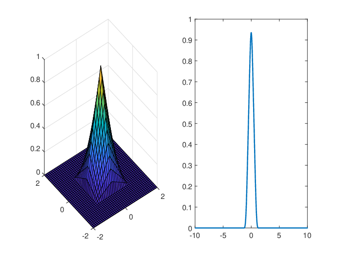
Figure 5.1. Left: the plot of ϕB\phi_{B}. Right: the plot of Radon transform P​ϕB​(x)P\phi_{B}(x) with P=[cos⁡(1.2208),sin⁡(1.2208)]P=[\cos(1.2208),\sin(1.2208)].

Refer to caption

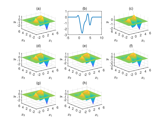
Figure 5.2. (a) The figure of f⁡(x1,x2)f(x_{1},x_{2}); (b) The figure of Radon transform P​fPf; (c) The reconstruction version f~​(x1,x2)\widetilde{f}(x_{1},x_{2}) when SNR=30; (d) The reconstruction version f~​(x1,x2)\widetilde{f}(x_{1},x_{2}) when SNR=35; (e) The reconstruction version f~​(x1,x2)\widetilde{f}(x_{1},x_{2}) when SNR=40; (f) The reconstruction version f~​(x1,x2)\widetilde{f}(x_{1},x_{2}) when SNR=45; (g) The reconstruction version f~​(x1,x2)\widetilde{f}(x_{1},x_{2}) when SNR=50; (h) The reconstruction version f~​(x1,x2)\widetilde{f}(x_{1},x_{2}) when SNR=55.

Without bias, we choose a function

(5.17) f=∑k1=04∑k2=04Ck1,k2​ϕB​(x1−k1,x2−k2)∈V⁡(ϕB)\displaystyle f=\sum^{4}_{k_{1}=0}\sum^{4}_{k_{2}=0}C_{k_{1},k_{2}}\phi_{B}(x_{1}-k_{1},x_{2}-k_{2})\in V(\phi_{B})

being supported on [0,6]2[0,6]^{2}. Randomly choosing an angle θ\theta from (arctan⁡2,π/2)(\arctan 2,\pi/2), it follows from Theorem 4.3 that with probability 11, ff can be determined by its SP Radon samples {P​f​(P​k):k∈E̊}\{Pf(Pk):k\in\mathring{E}\} with E̊=[0,4]2∩ℤ2.\mathring{E}=[0,4]^{2}\cap\mathbb{Z}^{2}. For simplicity, by the lexicographic order E̊N\mathring{E}_{N} is denoted as {e1,…,e25}\{e_{1},\ldots,e_{25}\}. Then ff is determined through the linear equation system

(5.18) A​(Ce1,…,Ce25)T=(P​f​(P​e1),…,P​f​(P​e25))T,\displaystyle A\big(C_{e_{1}},\ldots,C_{e_{25}}\big)^{T}=\big(Pf(Pe_{1}),\ldots,Pf(Pe_{25})\big)^{T},

where A=(P​ϕB​(P​ej−P​el))j,l=125.A=(P\phi_{B}(Pe_{j}-Pe_{l})\Big)^{25}_{j,l=1}. In this simulation we choose θ=1.2208\theta=1.2208 and P=[cos⁡(1.2208),sin⁡(1.2208)]P=[\cos(1.2208),\sin(1.2208)]. The graphs of ϕB\phi_{B} and P​ϕB​(x)P\phi_{B}(x) are illustrated in Figure 5.2. We add the Gaussian noise ϵ∼N⁡(0,σ2)\epsilon\thicksim N(0,\sigma^{2}) to the samples on the right-hand side of (5.18), and what we observed is P​f​(P​el)=P​f​(P​el)+ϵPf(Pe_{l})=Pf(Pe_{l})+\epsilon. Here the variance σ2\sigma^{2} is chosen such that the desired signal to noise ratio (SNR) is expressed by

SNR=10log10(∥{Pf(Pel):l=1,…,25}∥2225​σ2).\displaystyle\begin{array}[]{lllllllllllllllll}\hbox{SNR}=10\log_{10}\Big(\frac{\|\{Pf(Pe_{l}):\ l=1,\ldots,25\}\|^{2}_{2}}{25\sigma^{2}}\Big).\end{array}

We consider the Tikhonov regularization problem

(5.20) arg⁡minC⁡‖A​C−(P​f​(P​e1)~,…,P​f​(P​e25)~)T‖2+α​‖C‖2,\displaystyle\arg\min_{C}\|AC-\big(\widetilde{Pf(Pe_{1})},\ldots,\widetilde{Pf(Pe_{25})}\big)^{T}\|_{2}+\alpha\|C\|_{2},

where the regularization parameter α\alpha satisfies the requirement in [7, Theorem 2.5]. In this simulation, α\alpha is chosen as in Table 1. The solution to (5.20) is

(5.21) C^=(α​I+A∗​A)−1​A∗​(P​f​(P​e1)~,…,P​f​(P​e25)~)T,\displaystyle\widehat{C}=(\alpha I+A^{*}A)^{-1}A^{*}\big(\widetilde{Pf(Pe_{1})},\ldots,\widetilde{Pf(Pe_{25})}\big)^{T},

where II is the identity matrix. For every SNR∈{30,35,40,45,50,55}\hbox{SNR}\in\{30,35,40,45,50,55\}, conduct (5.21) for 10001000 trials and the average of the 10001000 outputs is denoted by C^¯\bar{\widehat{C}}. Construct f~\widetilde{f} through (5.17) with (Ce1,…,Ce25)T(C_{e_{1}},\ldots,C_{e_{25}}\big)^{T} being replaced by C^¯\bar{\widehat{C}}. And the reconstruction error is defined as

(5.22) error=[∑k=080∑l=080(f~​(−2+0.1​k,−2+0.1​l)−f⁡(−2+0.1​k,−2+0.1​l))2]1/2[∑k=080∑l=080(f⁡(−2+0.1​k,−2+0.1​l))2]1/2.\displaystyle\hbox{error}=\frac{\Big[\sum^{80}_{k=0}\sum^{80}_{l=0}\big(\widetilde{f}(-2+0.1k,-2+0.1l)-f(-2+0.1k,-2+0.1l)\big)^{2}\Big]^{1/2}}{\Big[\sum^{80}_{k=0}\sum^{80}_{l=0}\big(f(-2+0.1k,-2+0.1l)\big)^{2}\Big]^{1/2}}.

The average errors corresponding to different choices of SNR are recorded in Table 1.

SNR 30 35 40 45 50 55
α\alpha 2​e−032e-03 2.5​e−042.5e-04 3.5​e−053.5e-05 2​e−062e-06 1.5​e−071.5e-07 9.4​e−089.4e-08
error 0.4255 0.2471 0.0924 0.0480 0.0290 0.0087
Table 1. The error vs SNR.

6. Conclusion

We establish the single-angle (SA) Radon samples based reconstruction for the compactly supported functions in refinable shift-invariant spaces (SIS). We prove that any compactly supported function in a general refinable SIS can be reconstructed by its Radon samples at an appropriate angle. We also investigate the SA reconstruction problem in a class of SISs generated by a class of refinable box-splines. It is proved that any compactly supported function in the SISs generated by such box-splines, can be reconstructed by the SA Radon samples at almost every angle in [0,2​π)[0,2\pi).

7. Appendix: Proof of Lemma 4.5

Since φ\varphi is even and real-valued, so is φ^\widehat{\varphi}. Consequently, Ax1,…,xnA_{x_{1},\ldots,x_{n}} is symmetric. Now we choose 0<ζ~≤ζ0<\tilde{\zeta}\leq\zeta such that φ^​(ξ)>0\widehat{\varphi}(\xi)>0 on [−ζ~,ζ~][-\tilde{\zeta},\tilde{\zeta}]. Then for any 0≠(c1,…,cn)∈ℂn\textbf{0}\neq(c_{1},\ldots,c_{n})\in\mathbb{C}^{n}, it follows from Lemma 4.4 that

∑k=1n∑l=1nck​c¯l​φ​(xk−xl)=(c1,…,cn)​Ax1,…,xn​(c1,…,cn)⋆=∫ℝφ^​(ξ)​|∑k=1nck​e−i​xk​ξ|2​𝑑ξ≥∫ζ~/2−ζ~/2φ^(ξ)|∑nk=1cke−i​xk​ξ|2dξ,\displaystyle\begin{array}[]{lllllllll}\displaystyle\sum^{n}_{k=1}\sum^{n}_{l=1}c_{k}\overline{c}_{l}\varphi(x_{k}-x_{l})&=(c_{1},\ldots,c_{n})A_{x_{1},\ldots,x_{n}}(c_{1},\ldots,c_{n})^{\star}\\ &\displaystyle=\int_{\mathbb{R}}\widehat{\varphi}(\xi)|\sum^{n}_{k=1}c_{k}e^{-\textbf{i}x_{k}\xi}|^{2}d\xi\\ &\geq\displaystyle\int^{\tilde{\zeta}/2}_{-\tilde{\zeta}/2}\widehat{\varphi}(\xi)|\sum^{n}_{k=1}c_{k}e^{-\textbf{i}x_{k}\xi}|^{2}d\xi,\end{array}

where in the inequality we use φ^​(ξ)≥0\widehat{\varphi}(\xi)\geq 0 for any ξ∈ℝ\xi\in\mathbb{R}. Since xk≠xjx_{k}\neq x_{j}, it follows from [34, Lemma 6.7] that {e−i​xk​ξ}k=1n\{e^{-\textbf{i}x_{k}\xi}\}^{n}_{k=1} is linear independent in the space L2([−ζ~/2,ζ~/2])L^{2}([-\tilde{\zeta}/2,\tilde{\zeta}/2]). Consequently, {e−i​xk​ξ}k=1n\{e^{-\textbf{i}x_{k}\xi}\}^{n}_{k=1} is a Riesz basis for its finitely spanning space {∑k=1ncke−i​xk​ξ:ck∈ℂ}⊆L2([−ζ~/2,ζ~/2])\{\sum^{n}_{k=1}c_{k}e^{-\textbf{i}x_{k}\xi}:c_{k}\in\mathbb{C}\}\subseteq L^{2}([-\tilde{\zeta}/2,\tilde{\zeta}/2]), and there exists λX,ζ~>0\lambda_{X,\tilde{\zeta}}>0 (depending on XX and ζ~\tilde{\zeta}) such that

(7.4) ∫−ζ~/2ζ~/2|∑k=1ncke−i​xk​ξ|2dξ≥λX,ζ~∥{ck}k=1n∥22.\displaystyle\int^{\tilde{\zeta}/2}_{-\tilde{\zeta}/2}|\sum^{n}_{k=1}c_{k}e^{-\textbf{i}x_{k}\xi}|^{2}d\xi\geq\lambda_{X,\tilde{\zeta}}\|\{c_{k}\}^{n}_{k=1}\|^{2}_{2}.

On the other hand, since φ∈C⁡(ℝ)\varphi\in C(\mathbb{R}) is compactly supported, then φ^∈C∞​(ℝ)\widehat{\varphi}\in C^{\infty}(\mathbb{R}). Therefore, min⁡{φ^​(ξ):ξ∈[−ζ,ζ]}\min\{\widehat{\varphi}(\xi):\xi\in[-\zeta,\zeta]\} exists and is positive. Consequently, combining (7) and (7.4) we have

∑k=1n∑l=1nck​c¯l​φ​(xk−xl)=(c1,…,cn)​Ax1,…,xn​(c1,…,cn)⋆≥λX,ζ~​‖{ck}k=1n‖22>0.\displaystyle\begin{array}[]{lllllllll}\displaystyle\sum^{n}_{k=1}\sum^{n}_{l=1}c_{k}\overline{c}_{l}\varphi(x_{k}-x_{l})&=(c_{1},\ldots,c_{n})A_{x_{1},\ldots,x_{n}}(c_{1},\ldots,c_{n})^{\star}\\ &\geq\lambda_{X,\tilde{\zeta}}\|\{c_{k}\}^{n}_{k=1}\|^{2}_{2}>0.\end{array}

Stated another way, the matrix Ax1,…,xnA_{x_{1},\ldots,x_{n}} is positive definite. Therefore, by (7) we have

∑k=1n∑l=1nck​c¯l​φ​(xk−xl)≥sup0<ζ~≤ζ{λX,ζ~​min⁡{φ^​(ξ):ξ∈U⁡(0,ζ~)}}​∑j=1n|cj|2.\displaystyle\begin{array}[]{lllllllll}\displaystyle\sum^{n}_{k=1}\sum^{n}_{l=1}c_{k}\overline{c}_{l}\varphi(x_{k}-x_{l})&\geq\displaystyle\sup_{0<\tilde{\zeta}\leq\zeta}\Big\{\lambda_{X,\tilde{\zeta}}\min\{\widehat{\varphi}(\xi):\xi\in U(0,\tilde{\zeta})\}\Big\}\sum^{n}_{j=1}|c_{j}|^{2}.\end{array}

Now we choose 0<Λ:=supζ~{λX,ζ~​min⁡{φ^​(ξ):ξ∈U⁡(0,ζ~)}}<∞0<\Lambda:=\sup_{\tilde{\zeta}}\Big\{\lambda_{X,\tilde{\zeta}}\min\{\widehat{\varphi}(\xi):\xi\in U(0,\tilde{\zeta})\}\Big\}<\infty to conclude the proof.

References

  • [1] A. Aldroubi, K. Gröchenig, Nonuniform sampling and reconstruction in shift-invariant spaces, SIAM Rev., 43, 585-620, 2001.
  • [2] A. Aldroubi, Q. Sun, W.S. Tang, Convolution, average sampling, and a Calderon resolution of the identity for shift-invariant spaces, J. Fourier Anal. Appl., 22, 215-244, 2005.
  • [3] N. Antipa, G. Kuo, R. Heckel, B. Mildenhall, E. Bostan, R. Ng, L. Waller, DiffuserCam: lensless single-exposure 33D imaging, Optica, 5, 1-9, 2018.
  • [4] N.D. Atreas, On a class of non-uniform average sampling expansions and partial reconstruction in subspaces of L2​(ℝ)L^{2}(\mathbb{R}), Adv. Comput. Math., 36(1), 21-38, 2012.
  • [5] L. de Carli, P. Vellucci, pp-Riesz bases in quasi shift invariant spaces, arXiv:1710.00702, Preprint.
  • [6] C. K. Chui, An Introduction to Wavelets, Academic Press, 1992.
  • [7] H. W. Engl, M. Hanke, and A. Neubauer, Regularization of Inverse Problems, Mathematics and Its Applications, 375, Kluwer, Dordrecht, 1996.
  • [8] A. Entezari, M. Nilchian, and M. Unser, A box spline calculus for the discretization of computed tomography reconstruction problems, IEEE Transactions on Medical Imaging, 31, 1532-1541, 2012.
  • [9] R. S. Feris, Volker Krueger, R. M. C. Junior, A wavelet subspace method for real-time face tracking, Real-Time Imaging, 10, 339-350, 2002.
  • [10] S. Fan, S. S-Dryden, J. Zhao, S. Gausmann, A. Schülzgen, G. Li, B. E. A. Saleh, Optical fiber refractive index profiling by iterative optical diffraction tomography, J. Lightwave Technol., 36(24), 5754-5763, 2018.
  • [11] K. Gröchenig, J. Stöckler, Gabor frames and totally positive functions, Duke Math. J., 162(6), 1003-1031, 2013.
  • [12] K. Hamm, J. Ledford, On the structure and interpolation properties of quasi shift-invariant spaces, Journal of Functional Analysis, 274, 1959-1992, 2018.
  • [13] B. Han, The projection method for multidimensional framelet and wavelet analysis, Math. Model. Nat. Phenom., 7(2), 32-59, 2012.
  • [14] B. Han, Construction of wavelets and framelets by the projection method, Int. J. Appl. Math. Appl., 1(1), 1-40, 2008.
  • [15] B. Han, Projectable multidimensional refinable functions and biorthogonal wavelets, Appl. Comput. Harmon. Anal., 13, 89-102, 2002.
  • [16] B. Han, Framelets and wavelets: Algorithms, analysis, and applications, Applied and Numerical Harmonic Analysis, Birkhäuser/Springer, Cham, 2017. xxxiii +724 pp.
  • [17] B. Han, T. Li, X. Zhuang, Directional compactly supported box spline tight framelets with simple geometric structure, Applied Mathematics Letters, 91, 213-219, 2019.
  • [18] B. Han, Vector cascade algorithms and refinable function vectors in Sobolev spaces, Journal of Approximation Theory, 124(1), 44-88, 2003.
  • [19] A. C. Kak, M. Slaney, Principles of Computerized Tomographic Imaging, SIAM, Philadelphia, PA, 2001.
  • [20] N. Karimi, S. Kazem, D. Ahmadian, H. Adibi, L.V. Ballestra, On a generalized Gaussian radial basis function: Analysis and applications, Engineering Analysis with Boundary Elements, 112, 46-57, 2020.
  • [21] G. Kerkyacharian, G. Kyriazis, E. L. Pennec, P. Petrushev, D. Picard, Inversion of noisy Radon transform by SVD based needlets, Applied and Computational Harmonic Analysis, 28, 24-45, 2010.
  • [22] M. K. Kim, Principles and techniques of digital holographic microscopy, SPIE Reviews, 1, 1-51, 2010.
  • [23] Y. X. Li, J. Wen, J. Xian, Reconstruction from convolution random sampling in local shift invariant spaces, Inverse Problems, 35(12), 125008, 2019.
  • [24] Y. Li, D. Han, S. Yang, G. Huang, Nonuniform sampling and approximation in Sobolev space from the perturbation of framelet system, SCIENCE CHINA Mathematics, 64, 351-372, 2021.
  • [25] Y. Li, S. Yang, D. Yuan, Bessel multiwavelet sequences and dual multiframelets in Sobolev spaces, Advances in Computational Mathematics, 38: 491-529, 2013.
  • [26] X. Lu, Y.Sun, G. Bai, Adaptive wavelet-Galerkin methods for limited angle tomography, Image and Vision Computing, 28, 696-703, 2010.
  • [27] R. Horisaki, K. Fujii, and J. Tanida, Diffusion-based single-shot diffraction tomography, Optics Letters, 44, 1964-1967, 2019.
  • [28] M. T. McCann, and M. Unser, High-quality parallel-ray X-ray CT back projection using optimized interpolation, IEEE Transactions on Image Processing, 26, 4639-4647, 2017.
  • [29] F. Natterer, The mathematics of computerized tomography, in: Classics Appl. Math., vol. 32, SIAM, Philadelphia, PA, 2001.
  • [30] F. Natterer, F. Wübbeling, Mathematical Methods in Image Reconstruction, SIAM, Philadelphia, PA, 2001.
  • [31] M. Ste´\acute{e}phane, A Wavelet Tour of Signal Processing, Elsevier Inc., 2009.
  • [32] Q. Sun, Local reconstruction for sampling in shift-invariant spaces, Advances in Computational Mathematics, 32, 335-352, 2010.
  • [33] Y. Tian, Y. Z. Li, Subspace dual super wavelet and Gabor frames, SCIENCE CHINA Mathematics, 60, 2429-2446, 2017.
  • [34] H. Wendland, Scattered data approximation, Cambridge University Press, 17, 2004.
  • [35] Y. Xu, A new approach to the reconstruction of images from Radon projections, Advances in Applied Mathematics, 36, 388-460, 2006.
  • [36] A. D. Yablon, Multi-wavelength optical fiber refractive index profiling by spatially resolved fourier transform spectroscopy, Journal of Lightwave Technology, 28, 360-364, 2010.