跳到论文正文
W Papers独立论文阅读器 arXiv:2102.13203 论文正文 计算阅读时间 · 0%
引用这篇论文根据当前论文元数据生成,正式投稿前建议核对。


License: arXiv.org perpetual non-exclusive license
arXiv:2102.13203v2 [math.FA] 23 Dec 2021

Recovery of regular ridge functions on the ball

Tatyana Zaitseva Thanks: Moscow Center for Fundamental and Applied Mathematics, Laboratory “High-dimensional Approximation and Applications” of Lomonosov Moscow State University. Email: zaitsevatanja@gmail.com    Yuri Malykhin Thanks: Steklov Mathematical Institute, Laboratory “High-dimensional Approximation and Applications” of Lomonosov Moscow State University. Corresponding author. Email: malykhin@mi-ras.ru    Konstantin Ryutin Thanks: Moscow Center for Fundamental and Applied Mathematics, Laboratory “High-dimensional Approximation and Applications” of Lomonosov Moscow State University. Email: kriutin@yahoo.com
Abstract

We consider the problem of the uniform (in L∞L_{\infty}) recovery of ridge functions f⁡(x)=φ⁡(⟨a,x⟩)f(x)=\varphi(\langle a,x\rangle), x∈B2nx\in B_{2}^{n}, using noisy evaluations y1≈f⁡(x1),…,yN≈f⁡(xN)y_{1}\approx f(x^{1}),\ldots,y_{N}\approx f(x^{N}). It is known that for classes of functions φ\varphi of finite smoothness the problem suffers from the curse of dimensionality: in order to provide good accuracy for the recovery it is necessary to make exponential number of evaluations. We prove that if φ\varphi is analytic in a neighborhood of [−1,1][-1,1] and the noise is very small, ε⩽exp⁡(−c​log2​n)\varepsilon\leqslant\exp(-c\log^{2}n), then there is an efficient algorithm that recovers ff with good accuracy using O⁡(n​log2​n)O(n\log^{2}n) function evaluations.

Keywords: Ridge functions, Curse of dimensionality, recovery of analytic functions

MSC: 41A10, 41A63, 65D15

1 Introduction

Ridge functions recovery.

We consider ridge functions (plane waves) on the ball B2n={x∈ℝn:|x|⩽1}B_{2}^{n}=\{x\in\mathbb{R}^{n}\colon|x|\leqslant 1\}, i.e. functions of the form f⁡(x)=φ⁡(⟨a,x⟩)f(x)=\varphi(\langle a,x\rangle), where a∈ℝna\in\mathbb{R}^{n}, |a|=1|a|=1 is a fixed vector and φ\varphi is a function on [−1,1][-1,1] (as usual, ⟨x,y⟩\langle x,y\rangle is the scalar product on ℝn\mathbb{R}^{n}). The problem is to recover ff from its NN noisy values at some points: y1≈f⁡(x1),…,yN≈f⁡(xN)y_{1}\approx f(x^{1}),\ldots,y_{N}\approx f(x^{N}). The recovery algorithm is allowed to choose points x1,…,xNx^{1},\ldots,x^{N} for function evaluation; the algorithm is called adaptive if the point xi+1x^{i+1} may depend on the previously obtained values y1,…,yiy_{1},\ldots,y_{i}. When we say that our algorithm makes an evaluation of the unknown function we mean that it prescribes the point and receives the approximate value of the function at this point.

The difficulty is that when log⁡N=o⁡(n)\log N=o(n), for any points x1,…,xN∈B2nx^{1},\ldots,x^{N}\in B_{2}^{n} there exists a unit vector aa such that maxj⁡|⟨a,xj⟩|=o⁡(1)\max_{j}|\langle a,x^{j}\rangle|=o(1), as n→∞n\to\infty. Therefore we can measure φ\varphi only in a small neighborhood of zero and we cannot distinguish a nontrivial function supported outside this neighborhood from the identically zero function. Therefore, if one knows only that φ\varphi is smooth, then any recovery method requires exponential (with respect to the dimension) number of evaluations.

In the theory of function recovery the number of function evaluations sufficient to recover the unknown function with a given accuracy is studied. If its dependence on the dimension is exponential, then it is called the curse of dimensionality. Results on the existence of recovery algorithms with a small number of evaluations (say, polynomially depending on the dimension of the space) or, conversely, that any algorithm requires a large (exponential) number of evaluations are actively studied within the Information-based Complexity theory. See [15] for some statements and results in this direction.

For r>0r>0 let Lip⁡(r)\mathrm{Lip}(r) be the class of functions g:[−1,1]→ℝg\colon[-1,1]\to\mathbb{R}, with m=⌈r−1⌉m=\lceil r-1\rceil continuous derivatives on [−1,1][-1,1], s.t. ‖g(j)‖∞⩽1\|g^{(j)}\|_{\infty}\leqslant 1, j=0,…,mj=0,\ldots,m, and g(m)g^{(m)} is (r−m)(r-m)–Hölder with constant 11.

The recovery in L∞L_{\infty} for smooth ridge functions on the cube,

f⁡(x)=φ⁡(⟨a,x⟩),x∈[−1,1]n,‖a‖1=1,φ:[−1,1]→ℝ,f(x)=\varphi(\langle a,x\rangle),\quad x\in[-1,1]^{n},\;\|a\|_{1}=1,\;\varphi\colon[-1,1]\to\mathbb{R}, (1)

was studied by A. Cohen, I. Daubechies, R. DeVore, G. Kerkyacharian, D. Picard in [3]. The authors assume that φ∈Lip⁡(r)\varphi\in\mathrm{Lip}(r) and the vector aa is nonnegative: ai⩾0a_{i}\geqslant 0, i=1,…,ni=1,\ldots,n. This condition is very restrictive and it permits to recover φ⁡(t)\varphi(t) at any point t∈[−1,1]t\in[-1,1] as: φ⁡(t)=f⁡(xt)\varphi(t)=f(x_{t}), xt:=(t,t,…,t)x_{t}:=(t,t,\ldots,t). The most interesting results in [3] were obtained under the additional restriction that aa is bounded in the weak-ℓpn\ell_{p}^{n} norm, p∈(0,1)p\in(0,1).

These studies were continued by B. Doerr and S. Mayer in [6]. They dropped the non-negativity condition and replaced weak-ℓp\ell_{p} condition by the following:

‖a‖p⩽Mfor some p∈(0,1) and M⩾1.\|a\|_{p}\leqslant M\quad\mbox{for some $p\in(0,1)$ and $M\geqslant 1$.} (2)

Let ℛ⁡(r,p,M)\mathcal{R}(r,p,M) be the class of ridge functions ff on the cube, (1), with φ∈Lip⁡(r)\varphi\in\mathrm{Lip}(r) and vector aa satisfying  (2). The algorithm from [6] gives an approximation f~\widetilde{f}, such that

supf∈ℛ⁡(r,p,M)(𝖤​‖f−f~‖∞2)1/2⩽C⁡(r,p,M)​(log⁡N)−r⁡(1/p−1)for N⩾n.\sup_{f\in\mathcal{R}(r,p,M)}(\mathsf{E}\|f-\widetilde{f}\|_{\infty}^{2})^{1/2}\leqslant C(r,p,M)(\log N)^{-r(1/p-1)}\quad\mbox{for $N\geqslant n$.}

On the other hand it was proven that without (2) we have the curse of dimensionality: a similar recovery error for the class of ridge functions of the form (1) with φ∈Lip⁡(r)\varphi\in\mathrm{Lip}(r) is at least ε0>0\varepsilon_{0}>0, when N⩽C​exp⁡(n/8)N\leqslant C\exp(n/8).

Let us consider ridge functions on the ball:

f⁡(x)=φ⁡(⟨a,x⟩),|a|=1,x∈B2n.f(x)=\varphi(\langle a,x\rangle),\quad|a|=1,\;x\in B_{2}^{n}.

The corresponding recovery problem, even in a more general setting, was considered by M. Fornasier, K. Schnass and J. Vybiral in [7]. They aim to recover functions of the form f⁡(x)=φ⁡(A​x)f(x)=\varphi(Ax), where AA is some fixed k×nk\times n matrix and φ\varphi is a function of kk variables. Let us restrict ourselves to the case k=1k=1 (ridge functions). The authors of [7] introduce the following quantity

α:=∫Sn−1|φ′​(⟨a,x⟩)|2​d​μSn−1​(x)\alpha:=\int_{S^{n-1}}|\varphi^{\prime}(\langle a,x\rangle)|^{2}\,d\mu_{S^{n-1}}(x) (3)

(it does not depend on aa). They proved that if aa satisfies (2) (the case of p=1p=1 is possible), φ∈C2\varphi\in C^{2} and α\alpha is not close to zero (e.g. |φ′​(0)||\varphi^{\prime}(0)| is separated from zero) then the efficient recovery of ff is possible. Roughly speaking, N≍(ω​α)−3N\asymp(\omega\alpha)^{-3} evaluations are sufficient in order to achieve the error ⩽ω\leqslant\omega with high probability (when p=1p=1). Later, H. Tyagi and V. Cevher in [21] managed to get rid of the condition (2).

We remark that the functions considered in our paper can be very small in the neighborhood of zero and the quantity α\alpha can also be very small. Given the admissible error ω\omega, the class of analytic functions contains a function with oscillation more than ω\omega, but α⩽exp⁡(−c​log⁡(1/ω)​log​n)\alpha\leqslant\exp(-c\log(1/\omega)\log n). This explains why we require the noise level to be subexponentially small (it is a drawback for practical applications).

In [13] different approximation characteristics for several classes of ridge functions on the ball were estimated. As a corollary the formal proof of the curse of dimensionality for the corresponding recovery problem was given.

A closely related problem in statistics is known as a “single index model regression”. We briefly describe its formulation. Suppose XX is a random vector in ℝn\mathbb{R}^{n} and YY is a random variable. It is assumed that the regression function f⁡(x)=𝖤⁡(Y|X=x)f(x)=\mathsf{E}(Y|X=x) has the form f⁡(x)=g⁡(⟨a,x⟩)f(x)=g(\langle a,x\rangle), i.e., it is a ridge function; in the language of statistics, such an assumption is called the single index model. It is required to construct a regression, i.e., approximate ff from a sample {(Xi,Yi)}i=1N\{(X_{i},Y_{i})\}_{i=1}^{N}. We note the following important distinctions between the regression problem and our problem: (1) we are not free to choose XiX_{i}; these points are a random sample from the distribution μX\mu_{X} unknown to us; (2) the error is measured in the L2​(μX)L_{2}(\mu_{X})-norm rather than in the uniform norm. See [8] for the statistical setting.

Ridge functions appear also in the study of neural networks; this connection (in the context of the approximation theory) is discussed in the paper [17]. Indeed, the output of a one-neuron neural network with the activation function σ\sigma is the ridge function: x↦σ⁡(⟨w,x⟩)x\mapsto\sigma(\langle w,x\rangle). Let us remark that the problem of almost-optimal fitting of neuron weights vector ww to a training set {(xi,yi)}i=1N\{(x_{i},y_{i})\}_{i=1}^{N} is NP-hard, see [19] (for ℓ2\ell_{2}-norm). However, this problem differs from our setting in many aspects.

We remark that the well-known Phase Retrieval Problem (see [4]) for real vectors can be reformulated as a particular case φ⁡(u)=u2\varphi(u)=u^{2} of the ridge function recovery problem. It is not easy to compare our results with the state of the art in the Phase Retrieval Problem since the settings are different (e.g. in the latter problem the focus is on non-adaptive measurements).

Many fundamental properties of the classes of ridge functions were studied by A.Pinkus and his co-authors. The recovery problem was considered in the paper [2]; see also the book [18]. We also recommend the survey [11]: it contains interesting results about the representation by sums of ridge functions and their approximation properties.

Regular ridge functions.

S.V. Konyagin (personal communication) suggested to consider the case of regular ridge functions on the ball, i.e. f⁡(x)=φ⁡(⟨a,x⟩)f(x)=\varphi(\langle a,x\rangle) with regular (analytic) φ\varphi.

The recovery for classes of analytic functions was actively studied since the 1960s. The main focus was on the best possible method. The details about the results can be found in [16]. In the Information-based Complexity field there are different results on tractability of integration and approximation problems for certain classes of analytic functions. We should mention the papers by J. Dick, P. Kritzer, F. Pillichshammer, H. Woźniakowski [9] and Vybiral [22].

In our paper we apply the recovery method and error estimates from [5]: an analytic function is extrapolated from its noisy evaluations on the grid using least-squares fitted algebraic polynomials.

Let H⁡(σ,Q)H(\sigma,Q) be the class of analytic functions φ\varphi in Πσ={z=t+iy:|t|⩽1+σ,|y|⩽σ}\Pi_{\sigma}=\{z=t+iy\colon|t|\leqslant 1+\sigma,|y|\leqslant\sigma\}, such that |φ⁡(z)|⩽Q|\varphi(z)|\leqslant Q in Πσ\Pi_{\sigma} and φ⁡(z)\varphi(z) is real–valued for real zz. For this class we do have a polynomial recovery algorithm provided the evaluation errors are sufficiently small.

Given a class Φ\Phi of functions φ:[−1,1]→ℝ\varphi\colon[-1,1]\to\mathbb{R}, we denote by ℛ⁡(Φ,B2n)\mathcal{R}(\Phi,B_{2}^{n}) the class of ridge functions f:B2n→ℝf\colon B_{2}^{n}\to\mathbb{R} of the form f⁡(x)=φ⁡(⟨a,x⟩)f(x)=\varphi(\langle a,x\rangle), where a∈ℝna\in\mathbb{R}^{n}, |a|=1|a|=1 and φ∈Φ\varphi\in\Phi.

Theorem.

Let n∈ℕn\in\mathbb{N}, σ∈(0,1]\sigma\in(0,1], Q⩾1Q\geqslant 1, δ∗∈(0,12)\delta_{*}\in(0,\frac{1}{2}), ω∗∈(0,12)\omega_{*}\in(0,\frac{1}{2}). There is a probabilistic adaptive algorithm: for any function f∈ℛ⁡(H⁡(σ,Q),B2n)f\in\mathcal{R}(H(\sigma,Q),B_{2}^{n}) it uses NN evaluations of ff with errors not exceeding ε\varepsilon, where

ε:=Q​exp⁡(−C⁡(σ)​log⁡(Q​n/ω∗)​log​n),\varepsilon:=Q\exp(-C(\sigma)\log(Qn/\omega_{*})\log n), (4)
N:=⌈C⁡(σ)​log2⁡(Q​n/ω∗)​(log⁡(1/δ∗)+n)⌉N:=\lceil C(\sigma)\log^{2}(Qn/\omega_{*})(\log(1/\delta_{*})+n)\rceil (5)

and outputs an approximation f~\widetilde{f}, such that with probability ⩾1−δ∗\geqslant 1-\delta_{*} we have

maxx∈B2n⁡|f~​(x)−f⁡(x)|⩽ω∗.\max_{x\in B_{2}^{n}}|\widetilde{f}(x)-f(x)|\leqslant\omega_{*}.

We remark that f~\widetilde{f} is of the form f~​(x)=φ~​(⟨a~,x⟩)\widetilde{f}(x)=\widetilde{\varphi}(\langle\widetilde{a},x\rangle), with φ~\widetilde{\varphi} an algebraic polynomial of degree not exceeding C⁡(σ)​log⁡(Q/ω∗)C(\sigma)\log(Q/\omega_{*}). The number of operations for the algorithm depends polynomially on nn, Q/ω∗Q/\omega_{*} and log⁡(1/δ∗)\log(1/\delta_{*}) for fixed σ\sigma.

The function ff is invariant under (a,φ⁡(x))↦(−a,φ⁡(−x))(a,\varphi(x))\mapsto(-a,\varphi(-x)). We recover either aa and φ\varphi or −a,φ⁡(−x)-a,\varphi(-x).

Corollary.

Let ϰ>0\varkappa>0. There is a polynomial algorithm that uses at most C⁡(σ,ϰ)​n​log2​nC(\sigma,\varkappa)n\log^{2}n evaluations of an unknown function f∈R⁡(H⁡(σ,Q),B2n)f\in R(H(\sigma,Q),B_{2}^{n}) with errors ⩽Q​exp⁡(−C⁡(σ,ϰ)​log2​n)\leqslant Q\exp(-C(\sigma,\varkappa)\log^{2}n) and outputs an approximation f~\widetilde{f}, such that ‖f~−f‖L∞​(B2n)⩽Q​n−ϰ\|\widetilde{f}-f\|_{L_{\infty}(B_{2}^{n})}\leqslant Qn^{-\varkappa} with probability ⩾1−2​e−n\geqslant 1-2e^{-n}.

We did not try to optimize all the steps of the algorithm. Our main point is the possibility of the effective (of polynomial complexity) recovery of regular ridge functions. We also developed a new method involving global properties of functions (the so-called embedding) and order statistics. These results were announced in [23].

In section 3 we discuss the numerical implementation of the algorithm. We remark that in the program we find embedding coefficients using an effective procedure that requires minimization of a polynomial, see (31).

Notations and useful facts.

By homogeneity we may assume that Q=1Q=1. Indeed, we will show that the algorithm works for Q=1Q=1. For a general Q⩾1Q\geqslant 1 (which is given), we can divide all evaluated values yky_{k} by QQ and apply our algorithm to recover f/Q∈H⁡(σ,1)f/Q\in H(\sigma,1) with error ω∗/Q\omega_{*}/Q.

Fix σ∈(0,1]\sigma\in(0,1]. We may further assume that nn is large enough and ω∗\omega_{*} and δ∗\delta_{*} are small enough. Indeed, suppose that our algorithm works for some n∘n^{\circ}, ω∗∘\omega_{*}^{\circ}, δ∗∘\delta_{*}^{\circ} and requires N∘N^{\circ} function evaluations with error ε∘\varepsilon^{\circ}. Then the same algorithm works also for any n⩽n∘n\leqslant n^{\circ} (we can treat the vector a∈Sn−1a\in S^{n-1} as a vector in Sn∘−1S^{n^{\circ}-1} by adding zero coordinates) ω∗⩾ω∗∘\omega_{*}\geqslant\omega_{*}^{\circ}, δ∗∘⩾δ∗\delta_{*}^{\circ}\geqslant\delta_{*}. Our Theorem holds for nn, ω∗\omega_{*}, δ∗\delta_{*} provided that the number of evaluations given by the expression (5) is at least N∘N^{\circ}, and ε\varepsilon from (4) is at most ε∘\varepsilon^{\circ}. This can be achieved if we take C⁡(σ)C(\sigma) large enough.

For the rest of the paper φ\varphi denotes some unknown function from H⁡(σ,1)H(\sigma,1), σ∈(0,1]\sigma\in(0,1], and aa the unknown vector of coefficients of the ridge function f⁡(x)=φ⁡(⟨a,x⟩)f(x)=\varphi(\langle a,x\rangle), x∈B2nx\in B_{2}^{n}, |a|=1|a|=1.

Different quantities that are produced by the algorithm will be denoted by variables with “tildes”: e.g. φ~i\widetilde{\varphi}_{i}, Δ~h,νi\widetilde{\Delta}^{i}_{h,\nu} (they depend on the taken samples of our function ff).

In the rest of the paper for any vector γ∈B2n\gamma\in B_{2}^{n} we denote vγ:=n1/2​⟨a,γ⟩,v_{\gamma}:=n^{1/2}\langle a,\gamma\rangle, and φ~γ\widetilde{\varphi}_{\gamma} is the approximation for the function φ⁡(vγ​t)\varphi(v_{\gamma}t) satisfying (6) (see the first step of the algorithm).

We will fix some constants b,B>0b,B>0; it is supposed that b−1b^{-1} and BB are large enough. Namely, they satisfy the condition (21) given below; in fact one can take b=0.01b=0.01, B=5B=5. We call a real number vv typical if b⩽|v|⩽Bb\leqslant|v|\leqslant B.

Let σ1:=σ​b4​B\sigma_{1}:=\sigma\frac{b}{4B}.

Throughout the paper tt and xx are real variables and zz denotes a complex variable. Therefore the set {|t|⩽h}\{|t|\leqslant h\} is a segment, and {|z|⩽h}\{|z|\leqslant h\} is a disk on the complex plane.

We denote by c,c1,…,C,C1,…c,c_{1},\ldots,C,C_{1},\ldots positive reals (their values may differ from line to line).

The functions from H⁡(σ,1)H(\sigma,1) are LσL_{\sigma}-Lipschitz on [−1,1][-1,1], and Lσ⩽C​σ−1L_{\sigma}\leqslant C\sigma^{-1} (the explicit dependence on σ\sigma is not important for us).

Let EρE_{\rho} be the ellipse with focii ±1\pm 1 and the sum of semi-axes ρ\rho. We note that the major semi-axis of EρE_{\rho} equals R=12​(ρ+ρ−1)R=\frac{1}{2}(\rho+\rho^{-1}); and we have ρ=R+R2−1\rho=R+\sqrt{R^{2}-1}. It is clear that E1+σ⊂ΠσE_{1+\sigma}\subset\Pi_{\sigma}. When we say that some function ψ\psi is analytic in EρE_{\rho} and |ψ|⩽C|\psi|\leqslant C there, we mean that it is analytic in the open domain bounded by EρE_{\rho} and the estimate holds in the closed domain.

We make use of different probabilistic notions and constructions. For any random variable ξ\xi we denote by 𝖫𝖺𝗐⁡(ξ)\mathsf{Law}(\xi) its distribution. Φ\Phi denotes the distribution function of the standard gaussian random variable; by Φ∗\Phi^{*} we denote the distribution function of |ξ||\xi|, ξ∼𝒩⁡(0,1)\xi\sim\mathcal{N}(0,1), i.e. Φ∗​(x)=2​(Φ⁡(x)−1/2)\Phi^{*}(x)=2(\Phi(x)-1/2), x⩾0x\geqslant 0.

For describing the algorithm and estimating its accuracy we use (global) parameters N1N_{1}, N2N_{2}, N3N_{3}, MM, M1M_{1} (sufficiently large natural numbers) and ω1\omega_{1}, ω2\omega_{2}, ω3\omega_{3} (sufficiently small positive reals) that will be chosen in order to satisfy different inequalities required for our algorithm. All of them may depend on σ\sigma, nn, ω∗\omega_{*}, with the sole exception of N2N_{2}, that depends only on δ∗\delta_{*}. The meaning of these parameters will be clear from the scheme of the algorithm given below.

The scheme of the recovery algorithm.

Here we describe the steps of the algorithm and the ideas behind them. We hope that it will help the reader to follow the detailed proofs given in the next section.

  1. 1.

    The procedure of extrapolation.

    Given a vector γ∈B2n\gamma\in B_{2}^{n}, we evaluate the function ff on the grid:

    yk≈f(γkN1)=φ(⟨a,γ⟩kN1),k=−N1,…,N1,y_{k}\approx f\left(\gamma\frac{k}{N_{1}}\right)=\varphi\left(\langle a,\gamma\rangle\frac{k}{N_{1}}\right),\quad k=-N_{1},\ldots,N_{1},

    where N1N_{1} is large enough. Let vγ:=n1/2​⟨a,γ⟩v_{\gamma}:=n^{1/2}\langle a,\gamma\rangle. Thus, φ⁡(vγ​t)\varphi(v_{\gamma}t) will be evaluated on the uniform grid in [−n−1/2,n−1/2][-n^{-1/2},n^{-1/2}]. We fit a polynomial of an appropriate degree MM to the obtained values by least squares and use it to extrapolate φ⁡(vγ​t)\varphi(v_{\gamma}t) to larger segments. We rely on the estimates from [5] to prove that the constructed function φ~γ\widetilde{\varphi}_{\gamma} gives an approximation with small enough error ω1\omega_{1}:

    |φ~γ​(t)−φ⁡(vγ​t)|⩽ω1,|t|⩽min⁡(1,σ2​|vγ|).|\widetilde{\varphi}_{\gamma}(t)-\varphi(v_{\gamma}t)|\leqslant\omega_{1},\quad|t|\leqslant\min(1,\frac{\sigma}{2|v_{\gamma}|}). (6)
  2. 2.

    The construction of φ~i\widetilde{\varphi}_{i}.

    We take N2N_{2} random vectors on the sphere: γ1,…,γN2\gamma^{1},\ldots,\gamma^{N_{2}}. For each γi\gamma^{i} we construct the function φ~i:=φ~γi\widetilde{\varphi}_{i}:=\widetilde{\varphi}_{\gamma^{i}}, that approximates φ⁡(vi​t)\varphi(v_{i}t), vi:=vγiv_{i}:=v_{\gamma^{i}}. As a result we obtain the set of functions {φ~i}i=1N2.\{\widetilde{\varphi}_{i}\}_{i=1}^{N_{2}}.

    Recall that a number vv is called typical if b⩽|v|⩽Bb\leqslant|v|\leqslant B. Typical viv_{i} are most convenient for us: we see from (6) that, first, they are informative, i.e., a rather large part of φ\varphi is recovered, and second, the functions φ~i\widetilde{\varphi}_{i} exhibit a “good” behaviour on a fairly large segment |t|⩽σ/(2​B)|t|\leqslant\sigma/(2B).

    Since our choice of γi\gamma^{i} is random, our algorithm is probabilistic. All other constructions and statements are true under condition (18) on γi\gamma^{i}, that holds with high probability. That condition implies, e.g., that most of the viv_{i} are typical.

  3. 3.

    The estimation of function oscillation.

    At this step we distinguish the case of a function φ\varphi close to a constant from the case of a function whose oscillation is large. We estimate the oscillation of functions φ~i\widetilde{\varphi}_{i} and obtain either

    Δσ1/4:=max|t|⩽σ1/4⁡|φ⁡(t)−φ⁡(0)|⩽ω2,\Delta_{\sigma_{1}/4}:=\max_{|t|\leqslant\sigma_{1}/4}|\varphi(t)-\varphi(0)|\leqslant\omega_{2}, (7)

    or the inequality

    Δσ1=max|t|⩽σ1⁡|φ⁡(t)−φ⁡(0)|⩾ω22.\Delta_{\sigma_{1}}=\max_{|t|\leqslant\sigma_{1}}|\varphi(t)-\varphi(0)|\geqslant\frac{\omega_{2}}{2}. (8)

    The inequality (7) for small enough ω2\omega_{2} leads to the global bound

    max|t|⩽1⁡|φ⁡(t)−φ⁡(0)|⩽ω∗2.\max_{|t|\leqslant 1}|\varphi(t)-\varphi(0)|\leqslant\frac{\omega_{*}}{2}. (9)

    Hence ff can be approximated by f⁡(0)f(0) and the algorithm stops. In the case of (8) we proceed to the next step.

  4. 4.

    The procedure of the search for the embedding φ~γ1↪φ~γ2\widetilde{\varphi}_{\gamma_{1}}\hookrightarrow\widetilde{\varphi}_{\gamma_{2}}.

    We do not know the values of vγv_{\gamma} but a simple idea helps us to approximate the ratio |vγ2|/|vγ1||v_{\gamma_{2}}|/|v_{\gamma_{1}}| for any pair of vectors γ1,γ2\gamma_{1},\gamma_{2}. Namely, if |vγ2|⩾|vγ1||v_{\gamma_{2}}|\geqslant|v_{\gamma_{1}}|, then from (6) it follows that φ~γ1(t)≈φ~γ2(±t/λ)\widetilde{\varphi}_{\gamma_{1}}(t)\approx\widetilde{\varphi}_{\gamma_{2}}(\pm t/\lambda) for some λ⩾1\lambda\geqslant 1. If this approximate equality holds then we call it an “embedding” φ~γ1↪φ~γ2\widetilde{\varphi}_{\gamma_{1}}\hookrightarrow\widetilde{\varphi}_{\gamma_{2}}. We show that if vγ1v_{\gamma_{1}} is typical, the corresponding λ\lambda can be found with high accuracy and |λ~​(φ~γ1,φ~γ2)−|vγ2||vγ1||⩽ω3|\widetilde{\lambda}(\widetilde{\varphi}_{\gamma_{1}},\widetilde{\varphi}_{\gamma_{2}})-\frac{|v_{\gamma_{2}}|}{|v_{\gamma_{1}}|}|\leqslant\omega_{3}.

  5. 5.

    The search for a typical vv. The goal of this step is to find an index i0i_{0}, such that vi0v_{i_{0}} is typical and |vi0|⩽3/4|v_{i_{0}}|\leqslant 3/4. We find all possible pairwise embeddings φ~i↪φ~j\widetilde{\varphi}_{i}\hookrightarrow\widetilde{\varphi}_{j} for the set of functions {φ~i}\{\widetilde{\varphi}_{i}\}. That allows us to compare (approximately) pairs |vi||v_{i}|, |vj||v_{j}| and analyze the order statistics of the set {|vi|}\{|v_{i}|\} in order to find vi0v_{i_{0}}.

  6. 6.

    The recovery of the vector aa. Using the function φ~i0\widetilde{\varphi}_{i_{0}} from the previous step we construct embeddings φ~i0↪φ~γ\widetilde{\varphi}_{i_{0}}\hookrightarrow\widetilde{\varphi}_{\gamma} for appropriate vectors γ\gamma (linear combinations of standard basis vectors eke_{k}), and we find approximate values of ak/|vi0|a_{k}/|v_{i_{0}}|, where aka_{k} are the coordinates of aa. As a result we obtain the approximation a~\widetilde{a} to the vector aa with error

    |a−a~|⩽C​ω3⩽ω∗2​Lσ.|a-\widetilde{a}|\leqslant C\omega_{3}\leqslant\frac{\omega_{*}}{2L_{\sigma}}. (10)
  7. 7.

    The recovery of φ\varphi. The good approximation for aa allows us to approximate φ⁡(t)\varphi(t) for any t∈[−1,1]t\in[-1,1]: φ⁡(t)≈f⁡(t​a~)\varphi(t)\approx f(t\widetilde{a}). We can compute φ\varphi on a sufficiently fine uniform grid of size 2​N3+12N_{3}+1 in [−1,1][-1,1] and apply the technique of [5] to approximate φ\varphi by the polynomial of degree M1M_{1}. As a result we get

    max|t|⩽1⁡|φ⁡(t)−φ~​(t)|⩽ω∗2.\max\limits_{|t|\leqslant 1}|\varphi(t)-\widetilde{\varphi}(t)|\leqslant\frac{\omega_{*}}{2}. (11)

Finally, we have f~​(x):=φ~​(⟨a~,x⟩)\widetilde{f}(x):=\widetilde{\varphi}(\langle\widetilde{a},x\rangle). We estimate the error of the approximation, using (10), (11) and the Lipschitz property of φ\varphi :

|f⁡(x)−f~​(x)|⩽|φ⁡(⟨a,x⟩)−φ⁡(⟨a~,x⟩)|+|φ⁡(⟨a~,x⟩)−φ~​(⟨a~,x⟩)|⩽⩽Lσ​|a−a~|+ω∗2⩽ω∗.|f(x)-\widetilde{f}(x)|\leqslant|\varphi(\langle a,x\rangle)-\varphi(\langle\widetilde{a},x\rangle)|+|\varphi(\langle\widetilde{a},x\rangle)-\widetilde{\varphi}(\langle\widetilde{a},x\rangle)|\leqslant\\ \leqslant L_{\sigma}|a-\widetilde{a}|+\frac{\omega_{*}}{2}\leqslant\omega_{*}.

2 The algorithm

In this section we describe the recovery algorithm and estimate its accuracy. The theorem follows from these considerations. Each subsection corresponds to one step of the algorithm.

2.1 The procedure of extrapolation

We will apply the following useful statement on extrapolation of analytic functions from their values on a uniform grid. Recall that EρE_{\rho} is the ellipse with focii ±1\pm 1 and the sum of semi-axes ρ\rho.

Lemma 1 (See. [5], Corollary 2, 4).

Let ψ\psi be analytic in EρE_{\rho} and |ψ⁡(z)|⩽Q|\psi(z)|\leqslant Q there; let the values yk=ψ⁡(k/N)+ξky_{k}=\psi(k/N)+\xi_{k}, k=−N,…,Nk=-N,\ldots,N be known with accuracy |ξk|⩽ε|\xi_{k}|\leqslant\varepsilon. Let pMp_{M} be the polynomial of degree not exceeding MM that minimizes ∑k=−NN|p⁡(k/N)−yk|2\sum_{k=-N}^{N}|p(k/N)-y_{k}|^{2}, and M⩽N/2M\leqslant\sqrt{N/2}. Then:

  • (i)

    interpolation: for |x|⩽1|x|\leqslant 1, we have

    |pM​(x)−ψ⁡(x)|⩽C​M3/2​(Q​ρ−Mρ−1+ε),|p_{M}(x)-\psi(x)|\leqslant CM^{3/2}\left(Q\frac{\rho^{-M}}{\rho-1}+\varepsilon\right), (12)

    with CC an absolute constant;

  • (ii)

    extrapolation: for |x|∈[1,12​(ρ+ρ−1))|x|\in[1,\frac{1}{2}(\rho+\rho^{-1})), we have

    |pM​(x)−ψ⁡(x)|⩽C⁡(Q⁡(M3/2ρ−1+r1−r)​rM+M3/2​(ρ​r)M​ε),|p_{M}(x)-\psi(x)|\leqslant C\left(Q\left(\frac{M^{3/2}}{\rho-1}+\frac{r}{1-r}\right)r^{M}+M^{3/2}(\rho r)^{M}\varepsilon\right), (13)

    with r=(|x|+x2−1)/ρr=(|x|+\sqrt{x^{2}-1})/\rho, and CC an absolute constant.

Proof.

The case (i) corresponds to Corollary 2 from [5], and the case (ii) to Corollary 4. We apply Theorems 3 and 4 from [5] in order to obtain necessary estimates for singular numbers. ∎

Let us recall the setup of our algorithm. We recover an unknown function f⁡(x)=φ⁡(⟨a,x⟩)f(x)=\varphi(\langle a,x\rangle) with analytic φ∈H⁡(σ,1)\varphi\in H(\sigma,1), from its noisy evaluations of accuracy ε\varepsilon.

Procedure (extrapolation).

Given any vector γ∈B2n\gamma\in B_{2}^{n}, we receive the values yk≈f⁡(γ​kN1)y_{k}\approx f(\gamma\frac{k}{N_{1}}), k=−N1,…,N1k=-N_{1},\ldots,N_{1}, take the polynomial pMp_{M} of degree ⩽M\leqslant M that minimizes ∑k=−N1N1|pM​(k/N1)−yk|2\sum_{k=-N_{1}}^{N_{1}}|p_{M}(k/N_{1})-y_{k}|^{2}, and output the function φ~γ​(t):=pM​(n1/2​t)\widetilde{\varphi}_{\gamma}(t):=p_{M}(n^{1/2}t).

Proposition 1.

Suppose that N1=2​M2N_{1}=2M^{2} and the inequalities hold:

M⩾C⁡(σ)​log⁡ω1−1,M\geqslant C(\sigma)\log\omega_{1}^{-1}, (14)
log⁡(1/ε)⩾C⁡(log⁡ω1−1+M​log⁡n).\log(1/\varepsilon)\geqslant C(\log\omega_{1}^{-1}+M\log n). (15)

Then the function φ~γ\widetilde{\varphi}_{\gamma} given by the extrapolation Procedure satisfies the inequality (6).

Proof.

In our procedure we evaluate values of the function ψ⁡(z)=φ⁡(u​z)\psi(z)=\varphi(uz), u:=⟨a,γ⟩u:=\langle a,\gamma\rangle, on the uniform grid {k/N1}k=−N1N1\{k/N_{1}\}_{k=-N_{1}}^{N_{1}} in [−1,1][-1,1]. One can rewrite the target inequality (6) in the following way:

|pM​(x)−ψ⁡(x)|⩽ω1,|x|⩽min⁡(n1/2,R/2),R:=σ/|u|.|p_{M}(x)-\psi(x)|\leqslant\omega_{1},\quad|x|\leqslant\min(n^{1/2},R/2),\quad R:=\sigma/|u|. (16)

We start with the case R⩾2R\geqslant 2. The function ψ\psi is analytic in the disk of radius RR. Therefore it is analytic in the disk of radius R1=min⁡(R,2​n1/2)R_{1}=\min(R,2n^{1/2}) and in the set Eρ1E_{\rho_{1}}, ρ1=R1+R12−1\rho_{1}=R_{1}+\sqrt{R_{1}^{2}-1}. We need an estimate valid for |x|⩽R1/2|x|\leqslant R_{1}/2. For such xx we have

r=|x|+x2−1ρ1⩽R1/2+R12/4−1R1+R12−1⩽12.r=\frac{|x|+\sqrt{x^{2}-1}}{\rho_{1}}\leqslant\frac{R_{1}/2+\sqrt{R_{1}^{2}/4-1}}{R_{1}+\sqrt{R_{1}^{2}-1}}\leqslant\frac{1}{2}.

In the (more difficult) case of extrapolation we apply (13) for ρ1\rho_{1}, Q=1Q=1, 1⩽|x|⩽R1/21\leqslant|x|\leqslant R_{1}/2, r⩽1/2r\leqslant 1/2. Since ρ1⩾R1⩾2\rho_{1}\geqslant R_{1}\geqslant 2 and ρ1⩽2​R1⩽4​n1/2\rho_{1}\leqslant 2R_{1}\leqslant 4n^{1/2}, we get

|pM​(x)−ψ⁡(x)|⩽C​M3/2​(2−M+(ρ1/2)M​ε)⩽C​M3/2​(2−M+(4​n)M/2​ε).|p_{M}(x)-\psi(x)|\leqslant CM^{3/2}(2^{-M}+(\rho_{1}/2)^{M}\varepsilon)\leqslant CM^{3/2}(2^{-M}+(4n)^{M/2}\varepsilon).

We want each summand not to exceed ω1/2\omega_{1}/2. Therefore the first summand imposes the condition on MM: C​M3/2​2−M⩽ω1/2CM^{3/2}2^{-M}\leqslant\omega_{1}/2, that holds under (14). The second summand imposes the condition (15). The estimate in the case |x|⩽1|x|\leqslant 1 (interpolation) can be done similarly, the conditions on MM and ε\varepsilon are weaker than in the extrapolation case.

Let us consider the case R<2R<2. Since we have to estimate |pM​(x)−ψ​(x)||p_{M}(x)-\psi(x)| for |x|⩽min⁡(n,R/2)<1|x|\leqslant\min(\sqrt{n},R/2)<1, we apply the interpolation error estimate (12). Since E1+σ⊂ΠσE_{1+\sigma}\subset\Pi_{\sigma}, we see that φ\varphi is analytic and bounded in E1+σE_{1+\sigma}; hence as |u|⩽1|u|\leqslant 1, the function ψ\psi is also analytic and bounded in this set. Using the inequality (12) for ρ=1+σ\rho=1+\sigma, we get the condition on MM: C​M3/2​(σ−1​(1+σ)−M+ε)⩽ω1/2CM^{3/2}(\sigma^{-1}(1+\sigma)^{-M}+\varepsilon)\leqslant\omega_{1}/2 that leads to (14). The requirement on ε\varepsilon is weaker than (15).

The inequality (16) is proven. ∎

2.2 The construction of φ~i\widetilde{\varphi}_{i}

We take N2N_{2} random vectors (uniformly) on the unit sphere: γ1,…,γN2∈Sn−1\gamma^{1},\ldots,\gamma^{N_{2}}\in S^{n-1}. For each γi\gamma^{i}, using the procedure described above we construct the function φ~i:=φ~γi\widetilde{\varphi}_{i}:=\widetilde{\varphi}_{\gamma^{i}}, that approximates φ⁡(vi​t)\varphi(v_{i}t), where vi:=vγi=n1/2​⟨a,γi⟩v_{i}:=v_{\gamma^{i}}=n^{1/2}\langle a,\gamma^{i}\rangle.

The statistics of viv_{i}.

Let us consider the sequence viv_{i}. We trivially have |vi|⩽n1/2|v_{i}|\leqslant n^{1/2}. We do not know the values of viv_{i} but we know their distribution: {vi}i=1N2\{v_{i}\}_{i=1}^{N_{2}} is a sample from the random variable V=n1/2​X1V=n^{1/2}X_{1}, where the vector X=(X1,…,Xn)X=(X_{1},\ldots,X_{n}) is uniformly distributed on the sphere Sn−1S^{n-1}. Let FnF^{n} be the distribution function of the r.v. |V||V|; F^N2n\widehat{F}^{n}_{N_{2}} be the empirical distribution function of the sequence |v1|,…,|vN2||v_{1}|,\ldots,|v_{N_{2}}| (a sample from the distribution FnF^{n}).

The distribution of VV is close to the gaussian distribution: 𝖫𝖺𝗐⁡(V)≈𝒩⁡(0,1)\mathsf{Law}(V)\approx\mathcal{N}(0,1). Let us denote by Φ\Phi and Φ∗\Phi^{*} the distribution functions of a standard gaussian variable ξ\xi and the variable |ξ||\xi|, respectively. It is known that (see, e.g., [10])

supx∈ℝ|Φ∗​(x)−Fn​(x)|⩽c/n.\sup_{x\in\mathbb{R}}|\Phi^{*}(x)-F^{n}(x)|\leqslant c/n. (17)

We estimate the difference between FnF^{n} and F^N2n\widehat{F}^{n}_{N_{2}} using the Dvoretzky-Kiefer-Wolfowitz inequality [12]:

𝖯⁡(supx∈ℝ|Fn​(x)−F^N2n​(x)|>λ)⩽2​exp⁡(−2​N2​λ2).\mathsf{P}(\sup_{x\in\mathbb{R}}|F^{n}(x)-\widehat{F}^{n}_{N_{2}}(x)|>\lambda)\leqslant 2\exp(-2N_{2}\lambda^{2}).

Let λ=1/300\lambda=1/300, then with probability 1−2exp(−N2/45000)1-2\exp(-N_{2}/45000) we have

supx∈ℝ|Fn​(x)−F^N2n​(x)|⩽1300.\sup_{x\in\mathbb{R}}|F^{n}(x)-\widehat{F}^{n}_{N_{2}}(x)|\leqslant\frac{1}{300}. (18)

From here on we assume that (18) holds. It happens with probability not less than 1−δ∗1-\delta_{*} if we take N2⩾C​ln⁡(2/δ∗)N_{2}\geqslant C\ln(2/\delta_{*}).

If nn is sufficiently large, then c/n⩽1/300c/n\leqslant 1/300 in (17) and from (17), (18) we get for any q2>q1>0q_{2}>q_{1}>0:

|1N2​#​{i:q1⩽|vi|⩽q2}−(Φ∗​(q2)−Φ∗​(q1))|⩽1100.\left|\frac{1}{N_{2}}\#\{i\colon q_{1}\leqslant|v_{i}|\leqslant q_{2}\}-(\Phi^{*}(q_{2})-\Phi^{*}(q_{1}))\right|\leqslant\frac{1}{100}. (19)

In the proof we will use the following approximate values for Φ∗\Phi^{*}: Φ∗​(2)=0.9544​…\Phi^{*}(2)=0.9544\ldots, Φ∗​(1/2)=0.3829​…\Phi^{*}(1/2)=0.3829\ldots, Φ∗​(0.75)=0.5467​…\Phi^{*}(0.75)=0.5467\ldots, Φ∗​(0.46)=0.3544​…\Phi^{*}(0.46)=0.3544\ldots, Φ∗​(0.62)=0.4647​…\Phi^{*}(0.62)=0.4647\ldots, Φ∗​(0.57)=0.4313​…\Phi^{*}(0.57)=0.4313\ldots.

In particular, from the inequality Φ∗​(2)−Φ∗​(1/2)>0.57\Phi^{*}(2)-\Phi^{*}(1/2)>0.57, we see:

1N2​#​{i:1/2⩽|vi|⩽2}>1/2.\frac{1}{N_{2}}\#\{i\colon 1/2\leqslant|v_{i}|\leqslant 2\}>1/2. (20)

Recall that we call a number vv typical, if b⩽|v|⩽Bb\leqslant|v|\leqslant B. The appropriate choice of bb and BB gives that the number of nontypical viv_{i} does not exceed 2 percents. Formally, we assume that the numbers b,Bb,B are such that

Φ∗​(B)−Φ∗​(b)>99100,\Phi^{*}(B)-\Phi^{*}(b)>\frac{99}{100}, (21)

and therefore we have

#⁡{i:b⩽|vi|⩽B}⩾98100​N2.\#\{i\colon b\leqslant|v_{i}|\leqslant B\}\geqslant\frac{98}{100}N_{2}. (22)

2.3 The estimation of function oscillation

We consider the oscillation of the function φ\varphi:

Δh:=max|t|⩽h⁡|φ⁡(t)−φ⁡(0)|.\Delta_{h}:=\max_{|t|\leqslant h}|\varphi(t)-\varphi(0)|.

In order to estimate it we replace φ\varphi with φ~i\widetilde{\varphi}_{i}, and the maximum over the segment with the maximum over the grid with some step ν>0\nu>0:

Δ~h,νi:=maxk:|k​ν|⩽h|φ~i(kν)−φ~i(0)|,i=1,…,N2.\widetilde{\Delta}_{h,\nu}^{i}:=\max_{k\colon|k\nu|\leqslant h}|\widetilde{\varphi}_{i}(k\nu)-\widetilde{\varphi}_{i}(0)|,\quad i=1,\ldots,N_{2}.

Let Δ~h,ν𝗆𝖾𝖽\widetilde{\Delta}_{h,\nu}^{\mathsf{med}} be the median of the sequence {Δ~h,νi}i=1N2\{\widetilde{\Delta}_{h,\nu}^{i}\}_{i=1}^{N_{2}}. Let us prove that if h⩽σ/4h\leqslant\sigma/4 and ν\nu is sufficiently small, say, ν⩽ω1​(2​Lσ)−1\nu\leqslant\omega_{1}(2L_{\sigma})^{-1}, then the inequality holds:

Δh/2−3​ω1⩽Δ~h,ν𝗆𝖾𝖽⩽Δ2​h+3​ω1.\Delta_{h/2}-3\omega_{1}\leqslant\widetilde{\Delta}_{h,\nu}^{\mathsf{med}}\leqslant\Delta_{2h}+3\omega_{1}. (23)

Indeed, let ii be such that 1/2⩽|vi|⩽21/2\leqslant|v_{i}|\leqslant 2. Since h⩽σ/4h\leqslant\sigma/4, the approximation (6) works for |t|⩽h|t|\leqslant h and we can replace φ~i\widetilde{\varphi}_{i} with φ\varphi:

|Δ~h,νi−maxk:|k​ν|⩽h|φ(vikν)−φ(0)||⩽2ω1.|\widetilde{\Delta}^{i}_{h,\nu}-\max_{k\colon|k\nu|\leqslant h}|\varphi(v_{i}k\nu)-\varphi(0)||\leqslant 2\omega_{1}.

Using the Lipschitz condition and the inequality |vi|⩽2|v_{i}|\leqslant 2, we get

|Δ|vi|​h−maxk:|k​ν|⩽h|φ(vikν)−φ(0)||⩽2Lσν⩽ω1|\Delta_{|v_{i}|h}-\max_{k\colon|k\nu|\leqslant h}|\varphi(v_{i}k\nu)-\varphi(0)||\leqslant 2L_{\sigma}\nu\leqslant\omega_{1}

the last inequality is true because of the restriction on ν\nu. From this |Δ~h,νi−Δ|vi|​h|⩽3​ω1|\widetilde{\Delta}^{i}_{h,\nu}-\Delta_{|v_{i}|h}|\leqslant 3\omega_{1}. Therefore for all ii such that 1/2⩽|vi|⩽21/2\leqslant|v_{i}|\leqslant 2 we have

Δh/2−3​ω1⩽Δ~h,νi⩽Δ2​h+3​ω1.\Delta_{h/2}-3\omega_{1}\leqslant\widetilde{\Delta}^{i}_{h,\nu}\leqslant\Delta_{2h}+3\omega_{1}.

Since it holds for more than a half of all indices ii, the last inequalities hold also for the median.

We will use (23) for h:=σ1/2h:=\sigma_{1}/2 (recall that σ1=σ​b4​B\sigma_{1}=\sigma\frac{b}{4B}) and ν:=ω1/(2​Lσ)\nu:=\omega_{1}/(2L_{\sigma}). If Δ~h,ν𝗆𝖾𝖽⩾ω2−3​ω1\widetilde{\Delta}^{\mathsf{med}}_{h,\nu}\geqslant\omega_{2}-3\omega_{1}, then

Δ2​h⩾Δ~h,ν𝗆𝖾𝖽−3​ω1⩾ω2−6​ω1⩾12​ω2\Delta_{2h}\geqslant\widetilde{\Delta}^{\mathsf{med}}_{h,\nu}-3\omega_{1}\geqslant\omega_{2}-6\omega_{1}\geqslant\frac{1}{2}\omega_{2}

(we assume ω2⩾12​ω1\omega_{2}\geqslant 12\omega_{1}). Therefore we obtain (8) and proceed to the next step of the algorithm. In the opposite case of Δ~h,ν𝗆𝖾𝖽<ω2−3​ω1\widetilde{\Delta}^{\mathsf{med}}_{h,\nu}<\omega_{2}-3\omega_{1} we have Δσ1/4⩽ω2\Delta_{\sigma_{1}/4}\leqslant\omega_{2} and we get (7). Let us derive the global bound (9).

Lemma 2.

Let ψ∈H⁡(σ,1)\psi\in H(\sigma,1), σ∈(0,1]\sigma\in(0,1], and let Δτ:=max|t|⩽τ⁡|ψ⁡(t)|\Delta_{\tau}:=\max_{|t|\leqslant\tau}|\psi(t)|, τ∈(0,1)\tau\in(0,1). Then the estimate holds

max|t|⩽1⁡|ψ⁡(t)|⩽A​Δτα,α=α⁡(σ,τ)∈(0,1),A=A⁡(σ,τ)>0.\max_{|t|\leqslant 1}|\psi(t)|\leqslant A\Delta_{\tau}^{\alpha},\quad\alpha=\alpha(\sigma,\tau)\in(0,1),\;A=A(\sigma,\tau)>0.
Proof.

It is known that: for functions analytic in EρE_{\rho} and bounded there by 11 for any MM there exists a polynomial pp of degree not exceeding MM, such that max|t|⩽1⁡|pM​(t)−ψ⁡(t)|⩽2​ρ−M/(ρ−1)\max_{|t|\leqslant 1}|p_{M}(t)-\psi(t)|\leqslant 2\rho^{-M}/(\rho-1) (see [1]). Since E1+σ⊂ΠσE_{1+\sigma}\subset\Pi_{\sigma}, we can take ρ=1+σ\rho=1+\sigma. In order to make the error of the approximation less than Δτ\Delta_{\tau}, we take the minimal MM such that (1+σ)−M⩽σ2​Δτ(1+\sigma)^{-M}\leqslant\frac{\sigma}{2}\Delta_{\tau}. Then |pM​(t)−ψ⁡(t)|⩽Δτ|p_{M}(t)-\psi(t)|\leqslant\Delta_{\tau} and |pM​(t)|⩽2​Δτ|p_{M}(t)|\leqslant 2\Delta_{\tau} for |t|⩽τ|t|\leqslant\tau.

We use Chebyshev’s inequality in the following form (see [14], p.233): let τ1=τ⁡(1+2​q)\tau_{1}=\tau(1+2q), q>0q>0, and PP be a real algebraic polynomial of degree MM, then we have

‖P‖C⁡[−τ1,τ1]‖P‖C⁡[−τ,τ]⩽TM​(τ1/τ)⩽(1+2​q+2​q+q2)M.\frac{\|P\|_{C[-\tau_{1},\tau_{1}]}}{\|P\|_{C[-\tau,\tau]}}\leqslant T_{M}(\tau_{1}/\tau)\leqslant(1+2q+2\sqrt{q+q^{2}})^{M}.

TMT_{M} is the classical Chebyshev polynomial of degree M.M. If q⩽1q\leqslant 1 then the last expression is less than (1+5​q)M(1+5\sqrt{q})^{M}; take q=c1​σ2q=c_{1}\sigma^{2} to make (1+5​q)⩽(1+σ)1/2(1+5\sqrt{q})\leqslant(1+\sigma)^{1/2} (it holds for sufficiently small c1c_{1} and σ<2\sigma<2). Then for our polynomial pMp_{M} we obtain

max|t|⩽τ1⁡|pM​(t)|⩽2​Δτ​(1+5​q)M=2​Δτ​(1+σ)M/2⩽C⁡(σ)​Δτ1/2.\max_{|t|\leqslant\tau_{1}}|p_{M}(t)|\leqslant 2\Delta_{\tau}(1+5\sqrt{q})^{M}=2\Delta_{\tau}(1+\sigma)^{M/2}\leqslant C(\sigma)\Delta_{\tau}^{1/2}.

Hence Δτ1⩽C⁡(σ)​Δτ1/2\Delta_{\tau_{1}}\leqslant C(\sigma)\Delta_{\tau}^{1/2} for τ1/τ=1+c1​σ2\tau_{1}/\tau=1+c_{1}\sigma^{2}. We iterate this construction, using points τ1,τ2,…\tau_{1},\tau_{2},\ldots, and obtain the required estimate on max|t|⩽1⁡|ψ⁡(t)|\max_{|t|\leqslant 1}|\psi(t)|. ∎

Applying the lemma to the function 12​(φ​(t)−φ​(0))\frac{1}{2}(\varphi(t)-\varphi(0)), we get the estimate (9) under condition

A⁡(σ,σ1/4)​(ω2/2)α⁡(σ,σ1/4)⩽ω∗/4.A(\sigma,\sigma_{1}/4)(\omega_{2}/2)^{\alpha(\sigma,\sigma_{1}/4)}\leqslant\omega_{*}/4. (24)

So, the algorithm stops with the approximation f≈f⁡(0)f\approx f(0) (here we require that ε⩽ω∗/2\varepsilon\leqslant\omega_{*}/2).

2.4 The procedure of search for the embedding φ~γ1↪φ~γ2\widetilde{\varphi}_{\gamma_{1}}\hookrightarrow\widetilde{\varphi}_{\gamma_{2}}

Definition.

We say that function h1h_{1} embeds into h2h_{2} with coefficient λ⩾1\lambda\geqslant 1 and accuracy δ⩾0\delta\geqslant 0 (the notation is: h1⸦⟶λ,δh2h_{1}\stackrel{{\scriptstyle\lambda,\,\delta}}{{\lhook\joinrel\longrightarrow}}h_{2}), when

max|t|⩽1⁡|h1​(t)−h2​(t/λ)|⩽δ.\max_{|t|\leqslant 1}|h_{1}(t)-h_{2}(t/\lambda)|\leqslant\delta.

We can similarly define the embedding h1⸦⟶λ,δ,νh2h_{1}\stackrel{{\scriptstyle\lambda,\,\delta,\,\nu}}{{\lhook\joinrel\longrightarrow}}h_{2} replacing the maximum over [−1,1][-1,1] with the maximum over the grid of step ν>0\nu>0:

maxk:|k​ν|⩽1|h1(kν)−h2(kν/λ)|⩽δ.\max_{k\colon|k\nu|\leqslant 1}|h_{1}(k\nu)-h_{2}(k\nu/\lambda)|\leqslant\delta.

General embedding.

Let us consider the following general situation.

Let gg be some function on [−R,R][-R,R] and v1,v2>0v_{1},v_{2}>0 be reals. We suppose that we have some approximations g~i\widetilde{g}_{i} to the functions gi​(t):=g⁡(vi​t)g_{i}(t):=g(v_{i}t):

|g~i​(t)−gi​(t)|⩽ωfor |t|⩽min⁡(1,R/vi),i=1,2.|\widetilde{g}_{i}(t)-g_{i}(t)|\leqslant\omega\quad\mbox{for $|t|\leqslant\min(1,R/v_{i})$},\quad i=1,2. (25)

We assume the functions g~i\widetilde{g}_{i} to be defined on [−1,1][-1,1]. The condition vi​|t|⩽Rv_{i}|t|\leqslant R is natural since the function gig_{i} is defined for such tt.

For any v1⩽Rv_{1}\leqslant R and any v2⩾v1v_{2}\geqslant v_{1} we have the embedding g1⸦⟶λ∘, 0g2g_{1}\stackrel{{\scriptstyle\lambda^{\circ},\,0}}{{\lhook\joinrel\longrightarrow}}g_{2}, where λ∘=v2/v1\lambda^{\circ}=v_{2}/v_{1}. Indeed, for |t|⩽1|t|\leqslant 1 we have |v1​t|⩽R|v_{1}t|\leqslant R, and therefore the functions g1​(t)g_{1}(t) and g2​(t/λ0)g_{2}(t/\lambda^{0}) are correctly defined and

g1​(t)=g⁡(v1​t)=g⁡(v2​t/λ0)=g2​(t/λ0).g_{1}(t)=g(v_{1}t)=g(v_{2}t/\lambda^{0})=g_{2}(t/\lambda^{0}).

The coefficient of embedding λ\lambda is uniquely defined in the case of a continuous function hh. It follows from the following simple fact: if hh is continuous and h⁡(θ​s)≡h⁡(s)h(\theta s)\equiv h(s) for some θ∈(0,1)\theta\in(0,1), then h⁡(s)≡h⁡(0)h(s)\equiv h(0). We need the quantitative analogue of this fact when the accuracy of our embedding is non-zero.

Lemma 3.

Let h:[−r,r]→ℂh\colon[-r,r]\to\mathbb{C} be an LL–Lipschitz function: |h⁡(s)−h⁡(t)|⩽L​|s−t||h(s)-h(t)|\leqslant L|s-t| and Δ:=max|t|⩽r⁡|h⁡(t)−h⁡(0)|\Delta:=\max_{|t|\leqslant r}|h(t)-h(0)|. If θ∈(0,1)\theta\in(0,1) and

max|t|⩽r⁡|h⁡(t)−h⁡(θ​t)|⩽δ⩽Δ/2,\max_{|t|\leqslant r}|h(t)-h(\theta t)|\leqslant\delta\leqslant\Delta/2,

then

|1−θ|<ln⁡(2​L​r/Δ)⌊Δ2​δ⌋.|1-\theta|<\frac{\ln(2Lr/\Delta)}{\lfloor\frac{\Delta}{2\delta}\rfloor}.
Proof.

Let Δ=|h⁡(t^)−h⁡(0)|\Delta=|h(\hat{t})-h(0)| for some t^\hat{t}. We see that

Δ=|h⁡(t^)−h⁡(0)|⩽∑j=0k−1|h⁡(θj+1​t^)−h⁡(θj​t^)|+|h⁡(θk​t^)−h⁡(0)|⩽k​δ+L​r​θk.\Delta=|h(\hat{t})-h(0)|\leqslant\sum_{j=0}^{k-1}|h(\theta^{j+1}\hat{t})-h(\theta^{j}\hat{t})|+|h(\theta^{k}\hat{t})-h(0)|\leqslant k\delta+Lr\theta^{k}.

Setting k=⌊Δ/(2​δ)⌋k=\lfloor\Delta/(2\delta)\rfloor we obtain θk⩾Δ/(2​L​r)\theta^{k}\geqslant\Delta/(2Lr) and

ln⁡(Δ/(2​L​r))⩽k​ln⁡θ=k​ln⁡(1−(1−θ))⩽−k⁡(1−θ).\ln(\Delta/(2Lr))\leqslant k\ln\theta=k\ln(1-(1-\theta))\leqslant-k(1-\theta).

∎

We can now state

Lemma 4.

Let 0<r<R0<r<R and g:[−R,R]→ℝg\colon[-R,R]\to\mathbb{R} be an LL–Lipschitz function, such that the condition (25) holds for some v1,v2,ω>0v_{1},v_{2},\omega>0; let λ∘:=v2/v1\lambda^{\circ}:=v_{2}/v_{1}. Suppose that v1∈[r,R/2]v_{1}\in[r,R/2]. Then for any λ⩾1\lambda\geqslant 1 we have:

  • (i)

    If v2⩾v1v_{2}\geqslant v_{1} and |λ−λ∘|⩽min⁡(ωR​L,12)|\lambda-\lambda^{\circ}|\leqslant\min(\frac{\omega}{RL},\frac{1}{2}), then g~1⸦⟶λ, 3​ωg~2\widetilde{g}_{1}\stackrel{{\scriptstyle\lambda,\,3\omega}}{{\lhook\joinrel\longrightarrow}}\widetilde{g}_{2}.

  • (ii)

    If g~1⸦⟶λ, 3​ω,νg~2\widetilde{g}_{1}\stackrel{{\scriptstyle\lambda,\,3\omega,\,\nu}}{{\lhook\joinrel\longrightarrow}}\widetilde{g}_{2}, L​ν​max⁡(v1,v2)⩽ωL\nu\max(v_{1},v_{2})\leqslant\omega, and

    Δr:=max|t|⩽r⁡|g⁡(t)−g⁡(0)|⩾14​ω,\Delta_{r}:=\max_{|t|\leqslant r}|g(t)-g(0)|\geqslant 14\omega,

    then

    |λ−λ∘|max⁡(λ,λ∘)⩽28​ω​Δr−1​ln⁡(2​L​r/Δr).\frac{|\lambda-\lambda^{\circ}|}{\max(\lambda,\lambda^{\circ})}\leqslant 28\omega\Delta_{r}^{-1}\ln(2Lr/\Delta_{r}).
Proof.

(i). Let t∈[−1,1]t\in[-1,1]. We apply the triangle inequality:

|g~1​(t)−g~2​(t/λ)|⩽|g~1​(t)−g1​(t)|⏟⩽ω+|g1​(t)−g2​(t/λ∘)|⏟=0++|g2​(t/λ∘)−g2​(t/λ)|⏟⩽L​v2​|1/λ−1/λ∘|⩽ω+|g2​(t/λ)−g~2​(t/λ)|⏟⩽ω⩽3​ω.|\widetilde{g}_{1}(t)-\widetilde{g}_{2}(t/\lambda)|\leqslant\underbrace{|\widetilde{g}_{1}(t)-g_{1}(t)|}_{\leqslant\omega}+\underbrace{|g_{1}(t)-g_{2}(t/\lambda^{\circ})|}_{=0}+\\ +\underbrace{|g_{2}(t/\lambda^{\circ})-g_{2}(t/\lambda)|}_{\leqslant Lv_{2}|1/\lambda-1/\lambda^{\circ}|\leqslant\omega}+\underbrace{|g_{2}(t/\lambda)-\widetilde{g}_{2}(t/\lambda)|}_{\leqslant\omega}\leqslant 3\omega.

The first term is bounded by ω\omega since (25) holds and min⁡(1,R/v1)=1\min(1,R/v_{1})=1. Next, g2​(t/λ∘)g_{2}(t/\lambda^{\circ}) is defined and equals g⁡(v1​t)=g1​(t)g(v_{1}t)=g_{1}(t). The third term is estimated using Lipschitz condition:

|g⁡(v2​t/λ∘)−g⁡(v2​t/λ)|⩽L​v2|1/λ−1/λ∘|=L​v2λ∘⋅λ−1​|λ−λ∘|⩽L​R2​λ−1​ωR​L<ω.|g(v_{2}t/\lambda^{\circ})-g(v_{2}t/\lambda)|\leqslant Lv_{2}|1/\lambda-1/\lambda^{\circ}|=\frac{Lv_{2}}{\lambda^{\circ}}\cdot\lambda^{-1}|\lambda-\lambda^{\circ}|\leqslant\frac{LR}{2}\lambda^{-1}\frac{\omega}{RL}<\omega.

Finally, note that g2​(t/λ)g_{2}(t/\lambda) is defined and the approximation g2≈g~2g_{2}\approx\widetilde{g}_{2} holds: indeed, we have λ⩾12​λ∘\lambda\geqslant\frac{1}{2}\lambda^{\circ} (as λ∘⩾1\lambda^{\circ}\geqslant 1 and |λ−λ∘|⩽12|\lambda-\lambda^{\circ}|\leqslant\frac{1}{2}), so

v2​|t|/λ⩽2​v2/λ∘=2​v1⩽R.v_{2}|t|/\lambda\leqslant 2v_{2}/\lambda^{\circ}=2v_{1}\leqslant R.

(ii). Consider the grid where we have the embedding: {tk=k​ν:|k​ν|⩽1}\{t_{k}=k\nu\colon|k\nu|\leqslant 1\}. Pick some t∈[−1,1]t\in[-1,1]. One can find a point tkt_{k} in the grid such that |tk|⩽|t||t_{k}|\leqslant|t| and |t−tk|⩽ν|t-t_{k}|\leqslant\nu. As in (i), we have a chain of inequalities:

|g1​(t)−g2​(t/λ)|⩽|g1​(t)−g1​(tk)|⏟⩽L​v1​ν⩽ω+|g1​(tk)−g~1​(tk)|⏟⩽ω+|g~1​(tk)−g~2​(tk/λ)|⏟⩽3​ω++|g~2​(tk/λ)−g2​(tk/λ)|⏟⩽ω+|g2​(tk/λ)−g2​(t/λ)|⏟⩽L​v2​ν/λ⩽ω⩽7​ω.|g_{1}(t)-g_{2}(t/\lambda)|\leqslant\underbrace{|g_{1}(t)-g_{1}(t_{k})|}_{\leqslant Lv_{1}\nu\leqslant\omega}+\underbrace{|g_{1}(t_{k})-\widetilde{g}_{1}(t_{k})|}_{\leqslant\omega}+\underbrace{|\widetilde{g}_{1}(t_{k})-\widetilde{g}_{2}(t_{k}/\lambda)|}_{\leqslant 3\omega}+\\ +\underbrace{|\widetilde{g}_{2}(t_{k}/\lambda)-g_{2}(t_{k}/\lambda)|}_{\leqslant\omega}+\underbrace{|g_{2}(t_{k}/\lambda)-g_{2}(t/\lambda)|}_{\leqslant Lv_{2}\nu/\lambda\leqslant\omega}\leqslant 7\omega.

The third term is estimated by the definition of the embedding g~1⸦⟶λ, 3​ω,νg~2\widetilde{g}_{1}\stackrel{{\scriptstyle\lambda,\,3\omega,\,\nu}}{{\lhook\joinrel\longrightarrow}}\widetilde{g}_{2}. The bounds for the two last terms are valid whenever the expressions g2​(tk/λ)g_{2}(t_{k}/\lambda) and g2​(t/λ)g_{2}(t/\lambda) are defined. For this, we need that v2​|t|/λ⩽Rv_{2}|t|/\lambda\leqslant R. So, we have obtained the following inequality:

|g⁡(v1​t)−g⁡(v2​t/λ)|⩽7​ωfor |t|⩽min⁡(1,R​λ/v2).|g(v_{1}t)-g(v_{2}t/\lambda)|\leqslant 7\omega\quad\mbox{for $|t|\leqslant\min(1,R\lambda/v_{2})$.} (26)

We consider two cases: λ>λ∘\lambda>\lambda^{\circ} and λ<λ∘\lambda<\lambda^{\circ} (if lambdas are equal, there is nothing to prove). If λ>λ∘\lambda>\lambda^{\circ}, we set θ=λ∘/λ<1\theta=\lambda^{\circ}/\lambda<1, s=v1​ts=v_{1}t, and from (26) we obtain

|g⁡(s)−g⁡(θ​s)|⩽7​ω|g(s)-g(\theta s)|\leqslant 7\omega

when |s|⩽v1​min⁡(1,R​λ/v2)|s|\leqslant v_{1}\min(1,R\lambda/v_{2}). Since R​λ/v2>R​λ∘/v2=R/v1>1R\lambda/v_{2}>R\lambda^{\circ}/v_{2}=R/v_{1}>1, the above inequality is true for |s|⩽v1|s|\leqslant v_{1}, hence for all |s|⩽r|s|\leqslant r.

In the second case, λ<λ∘\lambda<\lambda^{\circ}, the inequality (26) can be written as

|g⁡(θ~​s~)−g⁡(s~)|⩽7​ω,θ~:=λ/λ∘,s~:=v2​t/λ,|g(\tilde{\theta}\tilde{s})-g(\tilde{s})|\leqslant 7\omega,\quad\tilde{\theta}:=\lambda/\lambda^{\circ},\;\tilde{s}:=v_{2}t/\lambda,

and it holds for

|s~|⩽v2λ​min⁡(1,R​λv2)=min⁡(v2/λ,R).|\tilde{s}|\leqslant\frac{v_{2}}{\lambda}\min(1,\frac{R\lambda}{v_{2}})=\min(v_{2}/\lambda,R).

Since v2/λ>v2/λ∘=v1⩾rv_{2}/\lambda>v_{2}/\lambda^{\circ}=v_{1}\geqslant r, it holds for |s~|⩽r|\tilde{s}|\leqslant r.

Applying in both cases Lemma 3, we arrive at

|λ−λ∘|max⁡(λ,λ∘)⩽ln⁡(2​L​r/Δr)⌊Δr/(14​ω)⌋⩽28​ω​Δr−1​ln⁡(2​L​r/Δr).\frac{|\lambda-\lambda^{\circ}|}{\max(\lambda,\lambda^{\circ})}\leqslant\frac{\ln(2Lr/\Delta_{r})}{\lfloor\Delta_{r}/(14\omega)\rfloor}\leqslant 28\omega\Delta_{r}^{-1}\ln(2Lr/\Delta_{r}).

∎

Let us apply the general constructions in our setting. The role of the function gg is played by the function φ⁡(η​t)\varphi(\eta t), where η:=b​σ1−1\eta:=b\sigma_{1}^{-1}; also let r:=br:=b and R:=2​BR:=2B. Note that a typical viv_{i} satisfies |vi|∈[r,R/2]|v_{i}|\in[r,R/2], as required in Lemma 4 and also that we have the inequality (8), which bounds the oscillation of φ⁡(η​t)\varphi(\eta t) on the segment [−η​σ1,η​σ1]=[−b,b][-\eta\sigma_{1},\eta\sigma_{1}]=[-b,b], as required. The function φ⁡(η​t)\varphi(\eta t) is Lσ′L_{\sigma}^{\prime}–Lipschitz, Lσ′:=η​LσL_{\sigma}^{\prime}:=\eta L_{\sigma}.

Procedure (embedding).

For any pair of functions φ~γ1\widetilde{\varphi}_{\gamma_{1}}, φ~γ2\widetilde{\varphi}_{\gamma_{2}} we try to find λ∈[1,λmax]\lambda\in[1,\lambda^{\mathrm{max}}], λmax:=n1/2​b−1\lambda^{\mathrm{max}}:=n^{1/2}b^{-1}, such that

φ~γ1​(η​t)⸦⟶λ, 3​ω1,νφ~γ2​(η​t),\widetilde{\varphi}_{\gamma_{1}}(\eta t)\stackrel{{\scriptstyle\lambda,\,3\omega_{1},\,\nu}}{{\lhook\joinrel\longrightarrow}}\widetilde{\varphi}_{\gamma_{2}}(\eta t),

where ν=n−1/2(Lσ′)−1ω1\nu=n^{-1/2}(L_{\sigma}^{\prime})^{-1}\omega_{1}, we search for the parameter λ\lambda over the grid in [1,λmax][1,\lambda^{\mathrm{max}}] of step ω1/(B​Lσ′)\omega_{1}/(BL_{\sigma}^{\prime}). If we obtain an embedding with some λ\lambda, we set λ~​(φ~γ1,φ~γ2):=λ\widetilde{\lambda}(\widetilde{\varphi}_{\gamma_{1}},\widetilde{\varphi}_{\gamma_{2}}):=\lambda and write φ~γ1↪φ~γ2\widetilde{\varphi}_{\gamma_{1}}\hookrightarrow\widetilde{\varphi}_{\gamma_{2}}. Otherwise, we similarly try to embed φ~γ1​(−t)\widetilde{\varphi}_{\gamma_{1}}(-t) into φ~γ2\widetilde{\varphi}_{\gamma_{2}} and in the case of success we set λ~​(φ~γ1,φ~γ2):=λ\widetilde{\lambda}(\widetilde{\varphi}_{\gamma_{1}},\widetilde{\varphi}_{\gamma_{2}}):=\lambda and also write φ~γ1↪φ~γ2\widetilde{\varphi}_{\gamma_{1}}\hookrightarrow\widetilde{\varphi}_{\gamma_{2}}. If we fail to find such λ\lambda, we say that there is no embedding and denote this situation as φ~γ1↪̸φ~γ2\widetilde{\varphi}_{\gamma_{1}}\not\hookrightarrow\widetilde{\varphi}_{\gamma_{2}}.

Proposition 2.

Let vγ1v_{\gamma_{1}} be a typical number, the values ωi\omega_{i} satisfy the inequalities

ω2⩾28ω1,Cω1ω2−1ln(4Lσ′b/ω2)⩽ω3bn−1/2.\omega_{2}\geqslant 28\omega_{1},\quad C\omega_{1}\omega_{2}^{-1}\ln(4L_{\sigma}^{\prime}b/\omega_{2})\leqslant\omega_{3}bn^{-1/2}. (27)

If |vγ2|⩾|vγ1||v_{\gamma_{2}}|\geqslant|v_{\gamma_{1}}|, then φ~γ1↪φ~γ2\widetilde{\varphi}_{\gamma_{1}}\hookrightarrow\widetilde{\varphi}_{\gamma_{2}}. If φ~γ1↪φ~γ2\widetilde{\varphi}_{\gamma_{1}}\hookrightarrow\widetilde{\varphi}_{\gamma_{2}}, then |vγ2|⩾|vγ1|(1−ω3)|v_{\gamma_{2}}|\geqslant|v_{\gamma_{1}}|(1-\omega_{3}). In both cases |λ~​(φ~γ1,φ~γ2)−|vγ2||vγ1||⩽ω3|\widetilde{\lambda}(\widetilde{\varphi}_{\gamma_{1}},\widetilde{\varphi}_{\gamma_{2}})-\frac{|v_{\gamma_{2}}|}{|v_{\gamma_{1}}|}|\leqslant\omega_{3}.

Proof.

We apply Lemma 4 with g⁡(t)=φ⁡(η​t)g(t)=\varphi(\eta t), r=br=b, R=2​BR=2B, ω=ω1\omega=\omega_{1}, L=Lσ′L=L_{\sigma}^{\prime}, g~1​(t)=φ~γ1​(η​t)\widetilde{g}_{1}(t)=\widetilde{\varphi}_{\gamma_{1}}(\eta t), g~2​(t)=φ~γ2​(η​t)\widetilde{g}_{2}(t)=\widetilde{\varphi}_{\gamma_{2}}(\eta t). Note that the typical vγ1v_{\gamma_{1}} satisfies |vγ1|∈[r,R/2]|v_{\gamma_{1}}|\in[r,R/2]. Let vγ1>0v_{\gamma_{1}}>0, vγ2>0v_{\gamma_{2}}>0; other cases are similar. Recall the notation λ∘=vγ2/vγ1\lambda^{\circ}=v_{\gamma_{2}}/v_{\gamma_{1}}.

Let vγ2⩾vγ1v_{\gamma_{2}}\geqslant v_{\gamma_{1}}. We have λ∘⩽n1/2/b=λmax\lambda^{\circ}\leqslant n^{1/2}/b=\lambda^{\mathrm{max}}; therefore, we try to embed with some λ\lambda, |λ−λ∘|⩽ω1/(2​B​L)|\lambda-\lambda^{\circ}|\leqslant\omega_{1}/(2BL) (it is clear that ω1/(2​B​L)<1/2\omega_{1}/(2BL)<1/2). By Lemma 4, we get the embedding with accuracy ⩽3​ω1\leqslant 3\omega_{1} on the whole segment, hence also on the grid; thus, φ~γ1↪φ~γ2\widetilde{\varphi}_{\gamma_{1}}\hookrightarrow\widetilde{\varphi}_{\gamma_{2}}.

Now suppose that φ~γ1↪φ~γ2\widetilde{\varphi}_{\gamma_{1}}\hookrightarrow\widetilde{\varphi}_{\gamma_{2}}. Recall the inequality (8) obtained at the step 2. It gives the estimate for gg on the segment [−b,b][-b,b] since η​σ1=b\eta\sigma_{1}=b:

Δ=max|t|⩽b⁡|g⁡(t)−g⁡(0)|⩾12​ω2.\Delta=\max_{|t|\leqslant b}|g(t)-g(0)|\geqslant\frac{1}{2}\omega_{2}.

We may apply (ii) from Lemma 4; note that the condition ω2/2⩾14​ω1\omega_{2}/2\geqslant 14\omega_{1} is satisfied by (27). We obtain

|λ−λ∘|max⁡(λ,λ∘)⩽C​ω1​ω2−1​ln⁡(4​L​b/ω2)⩽ω3/λmax.\frac{|\lambda-\lambda^{\circ}|}{\max(\lambda,\lambda^{\circ})}\leqslant C\omega_{1}\omega_{2}^{-1}\ln(4Lb/\omega_{2})\leqslant\omega_{3}/\lambda^{\mathrm{max}}. (28)

Due to the construction, we have max⁡(λ,λ∘)⩽λmax\max(\lambda,\lambda^{\circ})\leqslant\lambda^{\mathrm{max}}, and consequently |λ−λ∘|⩽ω3|\lambda-\lambda^{\circ}|\leqslant\omega_{3}. Thus,

vγ2=vγ1​λ∘=vγ1​(λ−(λ−λ∘))⩾vγ1​(1−ω3).v_{\gamma_{2}}=v_{\gamma_{1}}\lambda^{\circ}=v_{\gamma_{1}}(\lambda-(\lambda-\lambda^{\circ}))\geqslant v_{\gamma_{1}}(1-\omega_{3}).

∎

2.5 The search for typical viv_{i}.

For all pairs i,j∈{1,…,N2}i,j\in\{1,\ldots,N_{2}\} we start the embedding procedure to search for possible embeddings φ~i↪φ~j\widetilde{\varphi}_{i}\hookrightarrow\widetilde{\varphi}_{j}. It will allow us to compare the values of different |vi||v_{i}| with the relative error ω3\omega_{3}. In the following we use the estimates (19), (22) and Proposition 2.

Let us calculate the numbers

Kj:=#⁡{i:φ~i↪φ~j}.K_{j}:=\#\{i\colon\widetilde{\varphi}_{i}\hookrightarrow\widetilde{\varphi}_{j}\}.

Denote by J0J_{0} the set of jj such that 0.4⩽Kj/N2⩽0.50.4\leqslant K_{j}/N_{2}\leqslant 0.5. Let us consider the set {vj,j∈J0}\{v_{j},j\in J_{0}\}.

Let us show that if j∈J0j\in J_{0}, then |vj|⩽0.75|v_{j}|\leqslant 0.75. Suppose the converse, let |vj|>0.75|v_{j}|>0.75. Use that Φ∗​(0.75)>0.54\Phi^{*}(0.75)>0.54; hence due to (19), there are at least 0.53​N20.53N_{2} indices ii, such that |vi|⩽0.75|v_{i}|\leqslant 0.75; there are at least 0.51​N20.51N_{2} typical numbers among them. Proposition 2 implies that all such φ~i\widetilde{\varphi}_{i} embed into φ~j\widetilde{\varphi}_{j}, this contradicts j∈J0j\in J_{0}.

Now we show that j∈J0j\in J_{0} implies |vj|⩾0.45|v_{j}|\geqslant 0.45. Let |vj|<0.45|v_{j}|<0.45 and φ~i↪φ~j\widetilde{\varphi}_{i}\hookrightarrow\widetilde{\varphi}_{j}. If viv_{i} is typical, then due to Proposition 2 we have |vi|⩽0.46|v_{i}|\leqslant 0.46 (we may assume that ω3\omega_{3} is small). The amount of such viv_{i} is at most N2​(Φ∗​(0.46)+0.01)⩽0.37​N2N_{2}(\Phi^{*}(0.46)+0.01)\leqslant 0.37N_{2}. The amount of non-typical viv_{i} is at most 0.02​N20.02N_{2}. Therefore, there are at most 0.39​N20.39N_{2} such ii, this contradicts j∈J0j\in J_{0}.

Arguing as above, we see that indices jj with |vj|∈[0.57,0.62]|v_{j}|\in[0.57,0.62] belong to J0J_{0}. Therefore, the set J0J_{0} is non-empty:

#​J0⩾N2​(Φ∗​(0.62)−Φ∗​(0.57)−0.01)⩾0.02​N2.\#J_{0}\geqslant N_{2}(\Phi^{*}(0.62)-\Phi^{*}(0.57)-0.01)\geqslant 0.02N_{2}.

We take an arbitrary i0∈J0i_{0}\in J_{0} and obtain |vi0|∈[0.45,0.75]|v_{i_{0}}|\in[0.45,0.75]. Moreover, vi0v_{i_{0}} is typical.

2.6 The recovery of the vector aa

Here we use the extrapolation and embedding procedures and also the function φ~i0\widetilde{\varphi}_{i_{0}} with typical |vi0|⩽3/4|v_{i_{0}}|\leqslant 3/4 constructed at the previous step.

For every k=1,…,nk=1,\ldots,n we try to embed φ~i0↪φ~ek\widetilde{\varphi}_{i_{0}}\hookrightarrow\widetilde{\varphi}_{e_{k}} and find the corresponding λ~\widetilde{\lambda} (using the embedding procedure). Since aa is a unit vector, for at least one kk we have n1/2​|ak|⩾1>|vi0|n^{1/2}|a_{k}|\geqslant 1>|v_{i_{0}}| and thus the embedding exists. Suppose that for the k=k∗k=k^{*} the corresponding λ~\widetilde{\lambda} is maximal. We have |n1/2|​ak∗|/|vi0|−λ~​(φ~i0,φ~ek∗)|⩽ω3|n^{1/2}|a_{k^{*}}|/|v_{i_{0}}|-\widetilde{\lambda}(\widetilde{\varphi}_{i_{0}},\widetilde{\varphi}_{e_{k^{*}}})|\leqslant\omega_{3}. Although |ak∗||a_{k^{*}}| is not necessarily maximal, in any case max⁡|ak|⩽1.01​|ak∗|\max|a_{k}|\leqslant 1.01|a_{k^{*}}|.

Without loss of generality we may assume that ak∗>0a_{k^{*}}>0. Indeed, as we already noticed in Introduction, the function ff is invariant under the substitution (a,φ⁡(x))↦(−a,φ⁡(−x))(a,\varphi(x))\mapsto(-a,\varphi(-x)).

Thus, we know the ratio n1/2​ak∗/|vi0|n^{1/2}a_{k^{*}}/|v_{i_{0}}| up to ω3\omega_{3}; let us determine similar ratios for all other kk. For a given kk consider the vector γ=0.9​ek∗+0.1​ek∈B2n\gamma=0.9e_{k^{*}}+0.1e_{k}\in B_{2}^{n}. Then

vγ=n1/2​⟨0.9​ek∗+0.1​ek,a⟩=n1/2​(0.9​ak∗+0.1​ak)>0.75⩾|vi0|,v_{\gamma}=n^{1/2}\langle 0.9e_{k^{*}}+0.1e_{k},a\rangle=n^{1/2}(0.9a_{k^{*}}+0.1a_{k})>0.75\geqslant|v_{i_{0}}|,

therefore there exists an embedding φ~i0↪φ~γ\widetilde{\varphi}_{i_{0}}\hookrightarrow\widetilde{\varphi}_{\gamma} and |λ~​(φ~i0,φ~γ)−vγ/|vi0||⩽ω3|\widetilde{\lambda}(\widetilde{\varphi}_{i_{0}},\widetilde{\varphi}_{\gamma})-v_{\gamma}/|v_{i_{0}}||\leqslant\omega_{3} holds. From the equality n1/2​ak=−9​n1/2​ak∗+10​vγn^{1/2}a_{k}=-9n^{1/2}a_{k^{*}}+10v_{\gamma} and from the obtained inequalities on λ~​(φ~i0,φ~γ),λ~​(φ~i0,φ~ek∗)\widetilde{\lambda}(\widetilde{\varphi}_{i_{0}},\widetilde{\varphi}_{\gamma}),\widetilde{\lambda}(\widetilde{\varphi}_{i_{0}},\widetilde{\varphi}_{e_{k^{*}}}) it follows that

|n1/2​ak|vi0|−10​λ~​(φ~i0,φ~γ)+9​λ~​(φ~i0,φ~ek∗)|⩽C​ω3.\left|\frac{n^{1/2}a_{k}}{|v_{i_{0}}|}-10\widetilde{\lambda}(\widetilde{\varphi}_{i_{0}},\widetilde{\varphi}_{\gamma})+9\widetilde{\lambda}(\widetilde{\varphi}_{i_{0}},\widetilde{\varphi}_{e_{k^{*}}})\right|\leqslant C\omega_{3}.

Thus, we approximate coordinatewise the vector n1/2​a/|vi0|n^{1/2}a/|v_{i_{0}}| by a vector ww (the coordinates of ww are determined from the previous inequality) with the accuracy O⁡(ω3)O(\omega_{3}). So, we have |w−n1/2​a/|vi0||⩽C​n1/2​ω3|w-n^{1/2}a/|v_{i_{0}}||\leqslant Cn^{1/2}\omega_{3}. It is easy to see that

|w−r​a|⩽δ⇒|w|w|−a|⩽2​δr−δ,|w-ra|\leqslant\delta\quad\Rightarrow\quad\left|\frac{w}{|w|}-a\right|\leqslant\frac{2\delta}{r-\delta},

which implies that for a~:=w/|w|\widetilde{a}:=w/|w| we have |a~−a|⩽C​ω3|\widetilde{a}-a|\leqslant C\omega_{3}. We obtain (10). At this step we have used 2​n​(2​N1+1)2n(2N_{1}+1) additional evaluations (we needed the functions φ~ek\widetilde{\varphi}_{e_{k}} and φ~0.9​ek∗+0.1​ek\widetilde{\varphi}_{0.9e_{k^{*}}+0.1e_{k}}, 1⩽k⩽n1\leqslant k\leqslant n).

2.7 The recovery of φ\varphi

The knowledge of a~\widetilde{a} allows us to approximate φ\varphi at an arbitrary point of the segment [−1,1][-1,1]. Namely, for t∈[−1,1]t\in[-1,1] we evaluate ff at the point t​a~t\widetilde{a} and obtain the approximation yty_{t}: |yt−f⁡(t​a~)|=|yt−φ⁡(t⁡⟨a,a~⟩)|⩽ε|y_{t}-f(t\widetilde{a})|=|y_{t}-\varphi(t\langle a,\widetilde{a}\rangle)|\leqslant\varepsilon. Hence

|yt−φ⁡(t)|⩽|φ⁡(t⁡⟨a,a~⟩)−φ⁡(t)|+ε⩽Lσ​|a−a~|+ε⩽C​Lσ​ω3+ε;|y_{t}-\varphi(t)|\leqslant|\varphi(t\langle a,\widetilde{a}\rangle)-\varphi(t)|+\varepsilon\leqslant L_{\sigma}|a-\widetilde{a}|+\varepsilon\leqslant CL_{\sigma}\omega_{3}+\varepsilon;

where we applied the inequality |⟨a,a~⟩−1|⩽|a−a~|.|\langle a,\widetilde{a}\rangle-1|\leqslant|a-\widetilde{a}|. We use this method to obtain approximate values of φ\varphi on some grid {k/N3:k=−N3,…,N3}\{k/N_{3}\colon k=-N_{3},\ldots,N_{3}\}. Then we construct the polynomial pM1p_{M_{1}} of degree M1M_{1} using the least squares fit, as in the Step 1. Lemma 1 (i) gives us an estimate for the accuracy

|pM1​(x)−φ⁡(x)|⩽C1​M13/2​(ρ−M1ρ−1+Lσ​ω3+ε),−1⩽x⩽1.|p_{M_{1}}(x)-\varphi(x)|\leqslant C_{1}M_{1}^{3/2}(\frac{\rho^{-M_{1}}}{\rho-1}+L_{\sigma}\omega_{3}+\varepsilon),\quad-1\leqslant x\leqslant 1.

We can take ρ=1+σ\rho=1+\sigma. For our purposes it is sufficient that each of the summands is at most ω∗/6\omega_{*}/6. The first summand requires that M1⩾C⁡(σ)​log⁡(6/ω∗)M_{1}\geqslant C(\sigma)\log(6/\omega_{*}). The condition for the second summand is

ω3⩽ω∗C​LσM1−3/2.\omega_{3}\leqslant\frac{\omega_{*}}{CL_{\sigma}}M_{1}^{-3/2}. (29)

The condition on ε\varepsilon is

log⁡(1/ε)⩾log⁡(6/ω∗)+C​log⁡M1.\log(1/\varepsilon)\geqslant\log(6/\omega_{*})+C\log M_{1}. (30)

So we can put N3=2​M12N_{3}=2M_{1}^{2}. At this step we used 2​N3+12N_{3}+1 values of ff.

2.8 About the choice of parameters

We choose parameters in the following order:

  • •

    N2=⌈C​ln⁡(2/δ∗)⌉N_{2}=\lceil C\ln(2/\delta_{*})\rceil.

  • •

    M1=⌈C⁡(σ)​log⁡(2/ω∗)⌉M_{1}=\lceil C(\sigma)\log(2/\omega_{*})\rceil, N3=2​M12N_{3}=2M_{1}^{2}.

  • •

    We choose ω3\omega_{3} based on the condition (29). It automatically implies the condition on ω3\omega_{3} from (10).

  • •

    We choose ω2\omega_{2} based on condition (24).

  • •

    We choose ω1\omega_{1} based on inequality (27) and condition ω2⩾28​ω1\omega_{2}\geqslant 28\omega_{1}.

  • •

    We define MM by the condition (14) and suppose N1=2​M2N_{1}=2M^{2}.

  • •

    The main requirement on ε\varepsilon is (15) and (in fact, weaker) condition (30).

Total number of function evaluations equals N=(2​N1+1)​(N2+2​n)+2​N3+1N=(2N_{1}+1)(N_{2}+2n)+2N_{3}+1.

3 The implementation of the recovery algorithm

We implemented the recovery algorithm with some modifications using Python language and the numpy library. The code is available on Github: [24]. Let us describe the main changes that we introduced, and the results of numerical experiments.

The most important modification is related to the embedding procedure. The optimal parameter λ\lambda for embedding a polynomial p1​(t)p_{1}(t) into polynomial p2​(t)p_{2}(t) can be found as the solution of the problem min−1⩽μ⩽1⁡max|t|⩽1​|p1​(t)−p2​(μ​t)|\min\limits_{-1\leqslant\mu\leqslant 1}\max\limits_{|t|\leqslant 1}|p_{1}(t)-p_{2}(\mu t)|, where μ=1λ\mu=\frac{1}{\lambda}. Instead of the brute force search for possible μ\mu on the grid and the estimation of CC-norm, we consider the L2L_{2}-norm and explicitly find

min−1⩽μ⩽1⁡S⁡(μ),where ​S​(μ):=∫|t|⩽1(p1​(t)−p2​(μ​t))2​𝑑t.\min\limits_{-1\leqslant\mu\leqslant 1}S(\mu),\quad\mbox{where }S(\mu):=\int\limits_{|t|\leqslant 1}(p_{1}(t)-p_{2}(\mu t))^{2}\,dt. (31)

Indeed, S⁡(μ)S(\mu) is a polynomial itself and it can be minimized on the set {−1,1}∪{μ∈(−1,1):S′​(μ)=0}\{-1,1\}\cup\{\mu\in(-1,1)\colon S^{\prime}(\mu)=0\}. This approach allows us to effectively calculate rather accurate estimates of the embedding coefficient.

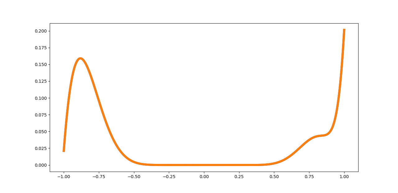
To test our algorithm we recover functions of the form

φ⁡(x):=xK1​(A02+∑k=1K2Ak​cos⁡(π​k​x)+Bk​sin⁡(π​k​x)).\varphi(x):=x^{K_{1}}\left(\frac{A_{0}}{\sqrt{2}}+\sum_{k=1}^{K_{2}}A_{k}\cos(\pi kx)+B_{k}\sin(\pi kx)\right). (32)

The values of parameters used in the program are given in the table below:

nεMM1N1N2N3K1K25010−2012302002520087\begin{array}[]{c|c|c|c|c|c|c|c|c|c}n&\varepsilon&M&M_{1}&N_{1}&N_{2}&N_{3}&K_{1}&K_{2}\\ \hline\cr 50&10^{-20}&12&30&200&25&200&8&7\\ \end{array}

We used the values of φ~γ​(t)\widetilde{\varphi}_{\gamma}(t) only for t∈[−n−1/2,n−1/2]t\in[-n^{-1/2},n^{-1/2}], i.e. only the interpolation was done (extrapolation was not required); the oscillation in our experiments was large enough to search for embeddings on the segment [−n−1/2,n−1/2][-n^{-1/2},n^{-1/2}] and find lambdas with high accuracy.

We note that the error ε\varepsilon is very small in our implementation since the values of the function φ\varphi near 00 are also very small. It is possible to increase the parameter ε\varepsilon but in this case we should decrease the degree K1K_{1}. Also, we can consider a relative error instead of an absolute error, in this case we can take it equal to e.g. 10−510^{-5}.

The following table contains the results of 1010 random experiments made with the parameters given above. In each experiment the vector of the coefficients of trigonometric polynomial defining φ\varphi by (32) and the vector aa of the ridge function were chosen randomly and uniformly from the unit spheres. We also specify the value of the α\alpha parameter (3).

#|a~−a|2‖φ~−φ‖Cα11.2691⋅10−54.7683⋅10−105.7276⋅10−724.5421⋅10−56.4352⋅10−93.4025⋅10−631.6969⋅10−46.3703⋅10−81.6590⋅10−649.2308⋅10−51.2412⋅10−81.5862⋅10−652.2896⋅10−73.0620⋅10−135.0647⋅10−666.1517⋅10−62.3048⋅10−109.2345⋅10−674.2528⋅10−66.8383⋅10−111.9411⋅10−685.4939⋅10−71.3600⋅10−122.5017⋅10−692.5037⋅10−64.3252⋅10−113.1520⋅10−7104.8359⋅10−52.6839⋅10−91.4242⋅10−6\begin{array}[]{c|c|c|c|c|c}\mbox{\#}&|\widetilde{a}-a|_{2}&\|\widetilde{\varphi}-\varphi\|_{C}&\alpha\\ \hline\cr 1&1.2691\cdot 10^{-5}&4.7683\cdot 10^{-10}&5.7276\cdot 10^{-7}\\ 2&4.5421\cdot 10^{-5}&6.4352\cdot 10^{-9}&3.4025\cdot 10^{-6}\\ 3&1.6969\cdot 10^{-4}&6.3703\cdot 10^{-8}&1.6590\cdot 10^{-6}\\ 4&9.2308\cdot 10^{-5}&1.2412\cdot 10^{-8}&1.5862\cdot 10^{-6}\\ 5&2.2896\cdot 10^{-7}&3.0620\cdot 10^{-13}&5.0647\cdot 10^{-6}\\ 6&6.1517\cdot 10^{-6}&2.3048\cdot 10^{-10}&9.2345\cdot 10^{-6}\\ 7&4.2528\cdot 10^{-6}&6.8383\cdot 10^{-11}&1.9411\cdot 10^{-6}\\ 8&5.4939\cdot 10^{-7}&1.3600\cdot 10^{-12}&2.5017\cdot 10^{-6}\\ 9&2.5037\cdot 10^{-6}&4.3252\cdot 10^{-11}&3.1520\cdot 10^{-7}\\ 10&4.8359\cdot 10^{-5}&2.6839\cdot 10^{-9}&1.4242\cdot 10^{-6}\\ \end{array}

The example of the function φ\varphi of the form  (32) is shown in the Fig. 1.

Refer to caption
Figure 1: The function φ\varphi (example)

4 Further work

Non-analytic functions.

Although the classes ℛ⁡(H⁡(σ,Q),B2n)\mathcal{R}(H(\sigma,Q),B_{2}^{n}) that we have considered are rich enough, e.g., they include polynomial ridge functions f⁡(x)=p⁡(⟨a,x⟩)f(x)=p(\langle a,x\rangle), it seems that the assumption that φ\varphi is analytic may be weakened.

The extrapolation technique of [5] may work for functions φ\varphi with certain restrictions on the order of the decay of sequences ‖φ(k)‖C⁡[−1,1]\|\varphi^{(k)}\|_{C[-1,1]} (as k→∞k\to\infty) or Ek​(f):=infdeg⁡p⩽k‖φ−p‖C⁡[−1,1]E_{k}(f):=\inf\limits_{\deg p\leqslant k}\|\varphi-p\|_{C[-1,1]}.

We also note that the embedding technique may work without extrapolation in some cases; a lower bound on the oscillation max|t|⩽h⁡|φ⁡(t)−φ⁡(0)|\max\limits_{|t|\leqslant h}|\varphi(t)-\varphi(0)|, h≈n−1/2h\approx n^{-1/2} is crucial here. Nevertheless we have to deal with the case of small oscillation (that was the goal of Step 3).

Derandomization.

Our algorithm is probabilistic, so the natural question is: can we get rid of the randomness? The only point where we need it is the condition (18). Let (X,μ)(X,\mu) be a probability space and 𝒞\mathcal{C} is some family of measurable subsets C⊂XC\subset X. Recall that the discrepancy of a finite set Γ\Gamma for a family 𝒞\mathcal{C} is defined as

disc⁡(Γ,𝒞):=supC∈𝒞|μ⁡(C)−|Γ∩C||Γ||.\mathrm{disc}(\Gamma,\mathcal{C}):=\sup_{C\in\mathcal{C}}\left|\mu(C)-\frac{|\Gamma\cap C|}{|\Gamma|}\right|.

The condition (18) is equivalent to the following discrepancy bound:

disc⁡({γi}i=1N2,𝒞n)⩽1300,\mathrm{disc}(\{\gamma_{i}\}_{i=1}^{N_{2}},\mathcal{C}_{n})\leqslant\frac{1}{300}, (33)

where 𝒞n\mathcal{C}_{n} is the set of symmetric spherical caps {γ∈Sn−1:|⟨a,γ⟩|>t}\{\gamma\in S^{n-1}\colon|\langle a,\gamma\rangle|>t\}. There are two difficulties: first, we need a bound for the discrepancy as n→∞n\to\infty; but the discrepancy theory is mostly developed for fixed nn. Second, we want a deterministic construction of {γi}\{\gamma_{i}\}. In the case of boxes ℛn\mathcal{R}_{n} in [0,1]n[0,1]^{n} it is known [20, Prop. 6.72] that there are constructive sets ΞN\Xi_{N} of NN points with

disc(ΞN,ℛn)⩽Cn3/2N−1/2ln1/2max(n,N).\mathrm{disc}(\Xi_{N},\mathcal{R}_{n})\leqslant Cn^{3/2}N^{-1/2}\ln^{1/2}\max(n,N).

So, N=n3+o⁡(1)N=n^{3+o(1)} points would suffice for small discrepancy. It is interesting to get good constructive bounds in the spherical case.

General ridge functions.

A ridge function is a simple yet interesting object, but in practice we have to deal with more complex functions. So it is important to study the recovery of generalized ridge functions, e.g., sums φ1​(⟨a1,x⟩)+φ2​(⟨a2,x⟩)+…+φr​(⟨ar,x⟩)\varphi_{1}(\langle a_{1},x\rangle)+\varphi_{2}(\langle a_{2},x\rangle)+\ldots+\varphi_{r}(\langle a_{r},x\rangle). One may consider the case of analytic (or even polynomial) functions φj\varphi_{j}.

Acknowledgement.

The authors wish to express their gratitude to S.V. Konyagin for his suggestion to consider the case of regular ridge functions and constant encouragement and to the anonymous referees for their careful work and precise comments.

References

  • [1] Bernstein, S.: Sur la meilleure approximation des fonctions continues par les polynomes du degré donné. II. Communications de la Société mathématique de Kharkow, 2-ée série 13, 145–194 (1912) (in Russian)
  • [2] Buhmann, M. D., Pinkus A.: Identifying linear combinations of ridge functions. Adv. Appl. Math. 22, 103–118 (1999)
  • [3] Cohen, A., Daubechies, I., DeVore, R., Kerkyacharian, G., Picard, D.: Capturing ridge functions in high dimensions from point queries. Constr. Approx. 35, 225–243 (2012)
  • [4] Casazza, P.G., Woodland, L.M.: Phase retrieval by vectors and projections. Operator Methods in Wavelets, Tilings, and Frames. Contemp. Math. 626, 1–7 (2014)
  • [5] Demanet, L., Townsend, A.: Stable extrapolation of analytic functions. Found. Comput. Math. 19, 297–331 (2019)
  • [6] Doerr, B., Mayer, S.: The recovery of ridge functions on the hypercube suffers from the curse of dimensionality. J. Complexity 63 (2021)
  • [7] Fornasier, M., Schnass, K., Vybiral, J.: Learning functions of few arbitrary linear parameters in high dimensions. Found. Comput. Math. 12, 229–262 (2012)
  • [8] Gaiffas, S., Lecue, G.: Optimal rates and adaptation in the single-index model using aggregation. Electron. J. Stat. 1, 538–573 (2007)
  • [9] Dick, J., Kritzer, P., Pillichshammer, F., Wo ’zniakowski, H.: Approximation of analytic functions in Korobov spaces. J. Complexity 30, 2–28 (2014)
  • [10] Khokhlov, V.I.: The uniform distribution on a sphere in ℝs\mathbb{R}^{s}. Properties of projections. I. Theory Probab. Appl. 50, 386–399 (2006)
  • [11] Konyagin, S. V., Kuleshov, A. A., Maiorov, V. E.: Some Problems in the Theory of Ridge Functions. Proc. Steklov Inst. Math. 301, 144–169 (2018)
  • [12] Massart, P.: The tight constant in the Dvoretzky–Kiefer–Wolfowitz inequality. Ann. Probab. 18, 1269–1283 (1990)
  • [13] Mayer, S., Ullrich, T., Vybiral, J.: Entropy and sampling numbers of classes of ridge functions. Constr. Approx. 42, 231–264 (2015)
  • [14] Natanson, I.P.: Constructive function theory, vol. 1, Ungar (1964)
  • [15] Novak, E., Wozniakowski, H.: Tractability of multivariate problems for standard and linear information in the worst case setting, Part I. J. Approx. Theory 207, 177–192 (2016)
  • [16] Osipenko, K.Yu: Optimal Recovery of Analytic Functions. Nova Publishers (2000)
  • [17] Pinkus, A.: Approximation theory of the MLP model in neural networks. Acta Numer. 8, 143–195 (1999)
  • [18] Pinkus, A.: Ridge Functions. Cambridge Tracts in Math. 205, Cambridge University Press, Cambridge (2015)
  • [19] Šíma, J.: Training a single sigmoidal neuron is hard. Neural Comput. 14, 2709–2728 (2002)
  • [20] Temlyakov, V.: Greedy Approximation. Cambridge University Press (2011)
  • [21] Tyagi, H., Cevher, V.: Learning non-parametric basis independent models from point queries via low-rank methods. Appl. Comput. Harmon. Anal. 37, 389–412 (2014)
  • [22] Vybíral, J.: Weak and quasi-polynomial tractability of approximation of infinitely differentiable functions. J. Complexity 30, 48–55 (2014)
  • [23] Zaitseva, T.I., Malykhin, Yu.V., Ryutin, K.S.: On Recovery of Regular Ridge Functions. Math. Notes 109, 307–311 (2021)
  • [24] https://github.com/TZZZZ/new_ridge_no_curse