跳到论文正文
W Papers独立论文阅读器 arXiv:2102.12958 论文正文 计算阅读时间 · 0%
引用这篇论文根据当前论文元数据生成,正式投稿前建议核对。


License: CC BY 4.0
arXiv:2102.12958v3 [math.SP] 29 Jul 2021

Analyticity of resolvents of elliptic operators on quantum graphs with small edges

D.I. Borisov
Abstract

We consider an arbitrary metric graph, to which we glue another graph with edges of lengths proportional to ε\varepsilon, where ε\varepsilon is a small positive parameter. On such graph, we consider a general self-adjoint second order differential operator ℋε\mathcal{H}_{\varepsilon} with varying coefficients subject to general vertex conditions; all coefficients in differential expression and vertex conditions are supposed to be analytic in ε\varepsilon. We introduce a special operator on a certain graph obtained by rescaling the aforementioned small edges and assume that it has no embedded eigenvalues at the threshold of its essential spectrum. Under such assumption, we show that certain parts of the resolvent of ℋε\mathcal{H}_{\varepsilon} are analytic in ε\varepsilon. This allows us to represent the resolvent of ℋε\mathcal{H}_{\varepsilon} by an uniformly converging Taylor-like series and its partial sums can be used for approximating the resolvent up to an arbitrary power of ε\varepsilon. In particular, the zero-order approximation reproduces recent convergence results by G. Berkolaiko, Yu. Latushkin, S. Sukhtaiev and by C. Cacciapuoti, but we additionally show that next-to-leading terms in ε\varepsilon-expansions of the coefficients in the differential expression and vertex conditions can contribute to the limiting operator producing the Robin part at the vertices, to which small edges are incident. We also discuss possible generalizations of our model including both the cases of a more general geometry of the small parts of the graph and a non-analytic ε\varepsilon-dependence of the coefficients in the differential expression and vertex conditions.

Keywords: graph, small edge, resolvent, analyticity, Taylor series, approximation

Institute of Mathematics, Ufa Federal Research Center, Russian Academy of Sciences, Ufa, Russia,

&

Bashkir State University, Ufa, Russia,

&

University of Hradec Králové, Hradec Králové, Czech Republic

borisovdi@yandex.ru

1 Introduction

The theory of quantum graphs or, in other words, the spectral theory of differential operators on graphs is actively developing nowadays and a rather new direction is devoted to studying quantum graphs with small edges. One of early studied problems came from the homogenization theory and it was devoted to models of woven membrane kind, see [9], [13]. The well-known result states that an elliptic operator on a graph looking as a net with small edges converge to a two-dimensional operator on an Euclidean domain approximated in a natural sense by such graph.

Another situation, which attracted quite a lot of attention, concerned the graphs with finitely many small edges. As a rather early publication on this subject we mention paper [8], in which it was shown that a general vertex condition in a graph can be approximated in the norm resolvent sense via ornamenting by small edges supporting a magnetic field and with delta-coupling at the vertices.

The case of a general graph with finitely small edges was addressed in [1]. On such graph, a Schrödinger operator subject to general vertex conditions was considered. The main result stated that under a certain non-resonance condition, see Condition 3.2 in [1], the considered operator converged in the norm resolvent sense to a Schrödinger operator on the limiting graph without small edges, which were replaced by certain conditions at the limiting vertices. The vertex conditions in [1] were described in terms of sympletic geometry and Lagrangian planes; the limiting vertex conditions were also formultated in the same terms. A similar study was made in [7], where there was considered a star graph, in which the vertex was replaced by a small rescaled finite graph. The operator on this perturbed graph was designed so that after the rescaling the small graph back to a finite size, the differential expression and vertex conditions turned out to be independent of a small parameter characterizing the size of the small graph. The main result of [7] provided the leading terms in the asymptotics for the perturbed resolvent and the estimates for the error term. The limiting condition at the vertex of the limiting star graph contained only the Neumann and Dirichlet parts.

The above described results motivated further studies of the graphs with small edges aimed on better understanding and describing the behavior of the resolvents. A natural question, apart of determining the limiting operator, is to find several next terms in the asymptotics for the resolvent or even its complete asymptotic expansion. This question was addressed in few recent papers [4], [5], [6] for some toy models represented by very simple graphs. A main feature of the considered models was the possibility of singular dependence of the coefficients in the differential expression on a small parameter governing the lengths of small edges. The main results obtained for these models stated that the resolvents were analytic in certain sense with respect to the small parameter and in the limit, the condition at the vertex to which the small edges shrank, could involve a Robin part. This Robin part was generated by the next-to-leading terms in the expansions of the coefficients of the differential expression with respect to the small parameter. For the resolvents, several first terms in their asymptotic expansions were found. The analytic dependence of the resolvent on the small parameter was in some sense surprising since small edges is an example of a singular perturbation and usually, while dealing with singular perturbation, one can hope only to find an asymptotic expansion for the resolvent but not to prove that this expansion is a converging Taylor series.

The present work is motivated by papers [1], [7]. We consider a general graph Γ\Gamma, to which a small graph γε\gamma_{\varepsilon} is glued. This small graph is obtained by rescaling a given graph γ\gamma into ε−1\varepsilon^{-1} times, where ε\varepsilon is a small parameter, see Figures 1, 2. On this perturbed graph with small edges we define a second order scalar differential operator ℋε\mathcal{H}_{\varepsilon} depending on ε\varepsilon. The differential expression is of a general form involving first order terms and varying coefficients. The vertex conditions are also of a general matrix form with arbitrary not necessarily unitary matrix coefficients. All coefficients in the differential expression and the vertex conditions depend arbitrarily on ε\varepsilon. For the coefficients in the vertex conditions and in the differential expression on non-small edges in Γ\Gamma, this dependence is analytic in ε\varepsilon, while the coefficients in the differential expression on the small edges in γε\gamma_{\varepsilon} are meromorphic in ε\varepsilon. On the coefficients in the differential expression and the vertex conditions of ℋε\mathcal{H}_{\varepsilon} we impose conditions ensuring the self-adjointness of this operator. Then we attach finitely many leads to the graph γ\gamma and denote such extended graph by γ∞\gamma_{\infty}, see Figure 2. On the graph γ∞\gamma_{\infty} we consider a self-adjoint operator ℋ∞\mathcal{H}_{\infty} with differential expression and vertex conditions generated in a certain way by those of the operator ℋε\mathcal{H}_{\varepsilon}. Our main assumption is that the operator ℋ∞\mathcal{H}_{\infty} has no embedded eigenvalues at the bottom of its essential spectrum; this does not exclude the presence of possible virtual levels at the same bottom. This assumption is of a similar nature as Non-resonance condition in work [1]. Under this condition, our main result states that the resolvent of the operator ℋε\mathcal{H}_{\varepsilon} is in some sense analytic in ε\varepsilon. Namely, we consider the restrictions of this resolvent to the graphs Γ\Gamma and γε\gamma_{\varepsilon} and the latter restriction then is sandwiched between the rescaling operators; such parts of the resolvent turn out to be analytic in ε\varepsilon. As a corollary, this provides a Taylor-like series for the resolvent. All these results are established for the resolvent of ℋε\mathcal{H}_{\varepsilon} regarded not only as operator acting in L2L_{2}, but also as acting from L2L_{2} into the Sobolev spaces W22W_{2}^{2} and into the spaces of continuous functions C2C^{2}.

The mentioned Taylor-like series for the resolvent allows us to find a limiting operator on the graph Γ\Gamma, the resolvent of which approximates the resolvent of ℋε\mathcal{H}_{\varepsilon} in the sense of the above norms. This is a convergence result as in [1] and [7] but for our general model. Similar to the toy models in [4], [5], [6], our general model also has a special feature related with the limiting vertex condition at M0M_{0}. Namely, we show that the next-to-leading terms in the ε\varepsilon-expansions of the coefficients in the differential expression and vertex conditions of ℋε\mathcal{H}_{\varepsilon} generate a Robin part in the limiting vertex conditions at a vertex M0M_{0}, through which the graph γε\gamma_{\varepsilon} is glued to the graph Γ\Gamma. Such case was excluded by the formulation of the problem in [7]. In [1], the Robin part could appear in the limit, but only due to the fact that, in our terms, the conditions at the vertices of the small edges were independent of ε\varepsilon.

Finally, we also conclude that despite the small edges are a singular perturbation, which can not be treated by means of the regular perturbation theory [11], the resolvent of the operator ℋε\mathcal{H}_{\varepsilon} depends analytically in ε\varepsilon and behaves similar to the situation, when the edges vary but do not vanish. The case with non-vanishing edges was considered in [3] and the main result stated that the resolvent of the Schrödinger operator on such graphs depended analytically on the edges lengths and the matrices involved in the vertex conditions.

Refer to caption
Figure 1: Examples of initial graphs Γ\Gamma and γ\gamma. The edges incident to M0M_{0} are split into three groups (n=3n=3).

In conclusion of this section, let us briefly describe the structure of the paper. In the next section we formulate the problem, our main assumptions and the main results. In the third section we discuss how far our results can be extended to the case, when several small graphs are glued to the graph Γ\Gamma, see Figure 4, including the case of the dependence on several independent small parameters. And we also discuss the case, when the assumed analyticity in the small parameter for the coefficients in the differential expression and vertex conditions is replaced by the infinite differentiability in ε\varepsilon or just by the existence of power asymptotic expansions. In the fourth section we discuss the self-adjointness of the operator we deal with. In the fifth section we introduce and study some auxiliary operator on γ\gamma, which is employed then in proving the main results in the sixth section.

2 Problem and main results

2.1 Problem

Let Γ\Gamma be a finite metric graph having no isolated vertices. The lengths of its edges can be both finite or infinite. We fix arbitrarily a vertex in the graph Γ\Gamma and denote it by M0M_{0}. The degree of this vertex is finite, that is, there exist finitely many edges ei\mathrm{e}_{i}, i=1,…,d0i=1,\ldots,d_{0} incident to M0M_{0}. Each loop in the family {ei}i=1,…,d0\{\mathrm{e}_{i}\}_{i=1,\ldots,d_{0}} is counted twice. By γ\gamma we denote one more graph, which is supposed to be finite, metric, having only edges of finite lengths and no isolated vertices or edges, see Figure 1.

Refer to caption
Figure 2: Graph Γε\Gamma_{\varepsilon} with a glued small graph and graph γ∞\gamma_{\infty}. The small edges in the graph Γε\Gamma_{\varepsilon} are indicated by thin lines. The leads in the graph γ∞\gamma_{\infty} are of light gray color.

Letting ε\varepsilon to be a small positive parameter, we scale each edge of the graph γ\gamma by ε\varepsilon and the resulting graph is denoted by γε\gamma_{\varepsilon}. More precisely, the vertices of the graph γε\gamma_{\varepsilon} are the same as those of γ\gamma, while each edge e∈γ\mathrm{e}\in\gamma is replaced by the edge of the length ε​|e|\varepsilon|\mathrm{e}|.

We chose arbitrary vertices MjM_{j}, j=1,…,nj=1,\ldots,n, in the graph γε\gamma_{\varepsilon} and then partition the aforementioned edges ei\mathrm{e}_{i}, i=1,…,d0i=1,\ldots,d_{0}, in the graph Γ\Gamma into nn non-empty groups {ei}i∈Jj\{\mathrm{e}_{i}\}_{i\in J_{j}}, j=1,…,nj=1,\ldots,n, where JjJ_{j} are some non-empty disjoint sets of indices and ⋃j=1nJj={1,…,d0}\bigcup\limits_{j=1}^{n}J_{j}=\{1,\ldots,d_{0}\}, 1⩽n⩽d01\leqslant n\leqslant d_{0}. Then we replace the vertex M0M_{0} in the graph Γ\Gamma by its nn copies, one copy for each group {ei}i∈Jj\{\mathrm{e}_{i}\}_{i\in J_{j}}. Finally, we introduce a graph, which will be the main object of our study, as the union of the graphs Γ\Gamma and γε\gamma_{\varepsilon}, where the vertices MjM_{j}, j=1,…,nj=1,\ldots,n, are identified with the aforementioned copies of the vertex M0M_{0} in the graph Γ\Gamma, see Figure 2. After the described gluing of the graphs Γ\Gamma and γε\gamma_{\varepsilon}, the edges eie_{i}, i=1,…,d0i=1,\ldots,d_{0}, are no longer connected at the vertex M0M_{0} but instead, each group {ei}i∈Jj\{\mathrm{e}_{i}\}_{i\in J_{j}} is incident to the vertex MjM_{j} in the graph γε\gamma_{\varepsilon}. Hereafter, we shall often identify the graphs Γ\Gamma and γε\gamma_{\varepsilon} with the corresponding subgraphs in Γε\Gamma_{\varepsilon}. In particular, in the sense of this identification, each function defined on Γε\Gamma_{\varepsilon} is also supposed to be defined on Γ\Gamma and γε\gamma_{\varepsilon} and vice versa. On each edge in Γ\Gamma and γ\gamma we fix a direction and consequently, a variable on it. Then the chosen direction is naturally transferred to the graph Γε\Gamma_{\varepsilon}.

The main object of our study is an unbounded operator ℋε\mathcal{H}_{\varepsilon} in L2​(Γε)L_{2}(\Gamma_{\varepsilon}) with a differential expression ℋ^​(ε)\hat{\mathcal{H}}(\varepsilon), the action of which is defined as

ℋ^​(ε)​u:=−dd​x​pε​d​ud​x+i⁡(dd​x​(qε​u)+qε​d​ud​x)+Vε​u,\hat{\mathcal{H}}(\varepsilon)u:=-\frac{d\ }{dx}p_{\varepsilon}\frac{du}{dx}+\mathrm{i}\left(\frac{d\ }{dx}(q_{\varepsilon}u)+q_{\varepsilon}\frac{du}{dx}\right)+V_{\varepsilon}u, (2.1)

where i\mathrm{i} is the imaginary unit and the coefficients are

pε:={pΓ​(⋅,ε)onΓ,𝒮εpγ​(⋅,ε)onγε,qε:={qΓ​(⋅,ε)onΓ,ε−1𝒮ε​qγ​(⋅,ε)onγε,Vε:={VΓ​(⋅,ε)onΓ,ε−2𝒮ε​Vγ​(⋅,ε)onγε.\begin{gathered}p_{\varepsilon}:=\left\{\begin{aligned} &p_{\Gamma}(\,\cdot\,,\varepsilon)&&\text{on}\quad\Gamma,\\ \mathcal{S}_{\varepsilon}&p_{\gamma}(\,\cdot\,,\varepsilon)&&\text{on}\quad\gamma_{\varepsilon},\end{aligned}\right.\qquad q_{\varepsilon}:=\left\{\begin{aligned} &q_{\Gamma}(\,\cdot\,,\varepsilon)&&\text{on}\quad\Gamma,\\ \varepsilon^{-1}&\mathcal{S}_{\varepsilon}q_{\gamma}(\,\cdot\,,\varepsilon)\quad&&\text{on}\quad\gamma_{\varepsilon},\end{aligned}\right.\\ V_{\varepsilon}:=\left\{\begin{aligned} &V_{\Gamma}(\,\cdot\,,\varepsilon)&&\text{on}\quad\Gamma,\\ \varepsilon^{-2}&\mathcal{S}_{\varepsilon}V_{\gamma}(\,\cdot\,,\varepsilon)&&\text{on}\quad\gamma_{\varepsilon}.\end{aligned}\right.\end{gathered} (2.2)

Here pΓ=pΓ​(⋅,ε)∈W∞1​(Γ)p_{\Gamma}=p_{\Gamma}(\,\cdot\,,\varepsilon)\in W_{\infty}^{1}(\Gamma), qΓ=qΓ​(⋅,ε)∈W∞1​(Γ)q_{\Gamma}=q_{\Gamma}(\,\cdot\,,\varepsilon)\in W_{\infty}^{1}(\Gamma), VΓ=VΓ​(⋅,ε)∈L2​(Γ)V_{\Gamma}=V_{\Gamma}(\,\cdot\,,\varepsilon)\in L_{2}(\Gamma) and pγ=pγ​(⋅,ε)∈W∞1​(γ)p_{\gamma}=p_{\gamma}(\,\cdot\,,\varepsilon)\in W_{\infty}^{1}(\gamma), qγ=qγ​(⋅,ε)∈W∞1​(γ)q_{\gamma}=q_{\gamma}(\,\cdot\,,\varepsilon)\in W_{\infty}^{1}(\gamma), Vγ=Vγ​(⋅,ε)∈L2​(γ)V_{\gamma}=V_{\gamma}(\,\cdot\,,\varepsilon)\in L_{2}(\gamma) are some real functions defined on the graphs Γ\Gamma and VγV_{\gamma} and these functions are analytic in ε\varepsilon in the sense of the norms in the mentioned spaces. The symbol 𝒮ε\mathcal{S}_{\varepsilon} stands for a linear operator mapping L2​(γ)L_{2}(\gamma) onto L2​(γε)L_{2}(\gamma_{\varepsilon}) by the rule

(𝒮ε​u)​(x):=u⁡(xε)asx∈eε(\mathcal{S}_{\varepsilon}u)(x):=u\left(\frac{x}{\varepsilon}\right)\quad\text{as}\quad x\in\mathrm{e}_{\varepsilon}

on each edge eε\mathrm{e}_{\varepsilon} in the graph γε\gamma_{\varepsilon}. We also assume an uniform ellipticity condition for the expression ℋ^​(ε)\hat{\mathcal{H}}(\varepsilon), namely, the existence of a fixed constant cℋ>0c_{\mathcal{H}}>0 independent of x∈Γx\in\Gamma, ξ∈γ\xi\in\gamma such that

pΓ​(x,0)⩾cℋa.e. onΓ,pγ​(ξ,0)⩾cℋa.e. onγp_{\Gamma}(x,0)\geqslant c_{\mathcal{H}}\quad\text{a.e. on}\quad\Gamma,\qquad p_{\gamma}(\xi,0)\geqslant c_{\mathcal{H}}\quad\text{a.e. on}\quad\gamma

Thanks to the assumed analyticity in ε\varepsilon, this condition implies the same condition for pΓ​(x,ε)p_{\Gamma}(x,\varepsilon) and pγ​(x,ε)p_{\gamma}(x,\varepsilon) for all sufficiently small ε\varepsilon with the constant cc replaced by c/2c/2.

The vertex conditions on the graph Γε\Gamma_{\varepsilon} are imposed as follows. Let MM be an arbitrary vertex in Γε\Gamma_{\varepsilon} of a degree d⁡(M)>0d(M)>0 and ei​(M)\mathrm{e}_{i}(M), i=1,…,d⁡(M)i=1,\ldots,d(M), be the edges incident to this vertex and ui:=u|ei​(M)u_{i}:=u\big|_{\mathrm{e}_{i}(M)}, i=1,…,d⁡(M)i=1,\ldots,d(M), be the restrictions of a function uu to the edges ei​(M)\mathrm{e}_{i}(M). We introduce two d⁡(M)d(M)-dimensional vectors

𝒰M​(u):=(u1​(M)ud⁡(M)​(M)),𝒰M′​(u):=(d​u1d​x1​(M)d​ud⁡(M)d​xd⁡(M)​(M)),\mathcal{U}_{M}(u):=\begin{pmatrix}u_{1}(M)\\ \vdots\\ u_{d(M)}(M)\end{pmatrix},\qquad\mathcal{U}_{M}^{\prime}(u):=\begin{pmatrix}\frac{du_{1}}{dx_{1}}(M)\\ \vdots\\ \frac{du_{d(M)}}{dx_{d(M)}}(M)\end{pmatrix}, (2.3)

where xix_{i} is the variable on the edge ei\mathrm{e}_{i}; this variable is chosen according the above discussed direction. At each vertex M∈ΓεM\in\Gamma_{\varepsilon} of a degree d⁡(M)>0d(M)>0 we impose a general vertex condition

AM​(ε)​𝒰M​(u)+BM​(ε)​𝒰M′​(u)=0,\mathrm{A}_{M}(\varepsilon)\mathcal{U}_{M}(u)+\mathrm{B}_{M}(\varepsilon)\mathcal{U}_{M}^{\prime}(u)=0, (2.4)

where AM​(ε)\mathrm{A}_{M}(\varepsilon) and BM​(ε)\mathrm{B}_{M}(\varepsilon) are some matrices of size d⁡(M)×d⁡(M)d(M)\times d(M) analytic in ε\varepsilon.

The matrices AM​(ε)\mathrm{A}_{M}(\varepsilon) and BM​(ε)\mathrm{B}_{M}(\varepsilon) in conditions (2.5) are defined non-uniquely up to the left multiplication by an arbitrary non-degenerate d⁡(M)×d⁡(M)d(M)\times d(M) matrix. In view of this fact, we denote r​(M):=rank⁡BM​(0)r(M):=\rank\mathrm{B}_{M}(0) and without loss of generality we additionally assume that for each M∈ΓεM\in\Gamma_{\varepsilon}, the first r⁡(M)r(M) rows in the matrix BM​(0)\mathrm{B}_{M}(0) are linearly independent and the other rows are zero, while each row among last d⁡(M)−r⁡(M)d(M)-r(M) ones in the matrix AM​(0)\mathrm{A}_{M}(0) is non-zero.

The domain of the operator ℋε\mathcal{H}_{\varepsilon} consists of the functions in W˙22​(γε)\dot{W}_{2}^{2}(\gamma_{\varepsilon}) satisfying the imposed vertex conditions; hereinafter, for an arbitrary graph we denote W˙2j(⋅):=⨁e∈⋅W2j(e)\dot{W}_{2}^{j}(\,\cdot\,):=\bigoplus\limits_{\mathrm{e}\in\,\cdot\,}W_{2}^{j}(\mathrm{e}), j=1,2j=1,2. The action of the operator ℋε\mathcal{H}_{\varepsilon} on such functions is defined by differential expression (2.1).

We want the introduced operator ℋε\mathcal{H}_{\varepsilon} to be self-adjoint and this is ensured by the two following assumptions. The first of them says that the matrix

AM​(ε)​ΠM−1​(ε)​BM∗​(ε)+iBM​(ε)​ΠM−1​(ε)​ΘM​(ε)​ΠM−1​(ε)​BM∗​(ε)\mathrm{A}_{M}(\varepsilon)\Pi_{M}^{-1}(\varepsilon)\mathrm{B}_{M}^{*}(\varepsilon)+\mathrm{i}\mathrm{B}_{M}(\varepsilon)\Pi_{M}^{-1}(\varepsilon)\Theta_{M}(\varepsilon)\Pi_{M}^{-1}(\varepsilon)\mathrm{B}_{M}^{*}(\varepsilon) (2.5)

is self-adjoint, where

ΠM​(ε):=diag⁡{νi​(M)​pε|ei​(M)​(M)}i=1,…,d⁡(M),\displaystyle\Pi_{M}(\varepsilon):=\diag\big\{\nu_{i}(M)p_{\varepsilon}\big|_{\mathrm{e}_{i}(M)}(M)\big\}_{i=1,\ldots,d(M)}, (2.6)
ΘM​(ε):=diag⁡{νi​(M)​qε|ei​(M)​(M)}i=1,…,d⁡(M),\displaystyle\Theta_{M}(\varepsilon):=\diag\big\{\nu_{i}(M)q_{\varepsilon}\big|_{\mathrm{e}_{i}(M)}(M)\big\}_{i=1,\ldots,d(M)},

and ei​(M)\mathrm{e}_{i}(M) are the edges incident to the vertex MM, while νi​(M):=1\nu_{i}(M):=1 if the inward direction on the edge ei​(M)\mathrm{e}_{i}(M) at the vertex MM coincides with the above chosen direction on this edge and νi​(M):=−1\nu_{i}(M):=-1 otherwise.

The second assumption is the rank condition rank⁡(AM​(0)​BM​(0))=d⁡(M)\rank\big(\mathrm{A}_{M}(0)\ \;\mathrm{B}_{M}(0)\big)=d(M) imposed at each vertex M∈ΓεM\in\Gamma_{\varepsilon}. In view of the above conditions for the structure of matrices AM\mathrm{A}_{M} and BM\mathrm{B}_{M}, this condition is obviously equivalent to

rank⁡(AM​(ε)​BM​(ε))=d⁡(M)\rank\big(\mathrm{A}_{M}(\varepsilon)\ \;\mathrm{B}_{M}(\varepsilon)\big)=d(M) (2.7)

for all sufficiently small ε\varepsilon.

2.2 Notation and assumption

To formulate our main results, we need some additional notations. By γ∞\gamma_{\infty} we denote a graph obtained by attaching leads (edges of infinite lengths) ei∞\mathrm{e}_{i}^{\infty}, i∈Jji\in J_{j}, j=1,…,nj=1,\ldots,n, to each vertex MjM_{j}, j=1,…,nj=1,\ldots,n, in the graph γ\gamma; the vertex MjM_{j} serves as the origin for the attached edges ei\mathrm{e}_{i}. The variable on the graph γ∞\gamma_{\infty} is denoted by ξ\xi.

The introduced graph appears in a very natural way. Namely, we consider the subgraph γε\gamma_{\varepsilon} in Γε\Gamma_{\varepsilon} with the edges ei\mathrm{e}_{i} incident to the vertices MjM_{j}. Then we rescale this subgraph and the edges by means of ε\varepsilon so that the graph γε\gamma_{\varepsilon} turns into the graph γ\gamma. Under such rescaling, the edges ei\mathrm{e}_{i} become ones with lengths of order O⁡(ε−1)O(\varepsilon^{-1}) and in the limit ε→+0\varepsilon\to+0, we just replace them by the leads ei∞\mathrm{e}_{i}^{\infty}.

The described scaling corresponds to the change of the variables ξ=x​ε−1\xi=x\varepsilon^{-1} and we need to see how the part of the operator ℋε\mathcal{H}_{\varepsilon} corresponding to γε\gamma_{\varepsilon} is transformed under such change. Namely, we first replace the coefficients of the differential expression ℋ^ε\hat{\mathcal{H}}_{\varepsilon} on the edges ei\mathrm{e}_{i} by their values at M0M_{0}. Then we multiply the obtained differential expression by ε2\varepsilon^{2}, pass to the variable ξ\xi and ε=0\varepsilon=0. This gives rise to the differential expression

ℋ^∞​u:=−dd​ξ​pγ​(⋅,0)​d​ud​ξ+i⁡(dd​ξ​(qγ​(⋅,0)​u)+qγ​(⋅,0)​d​ud​ξ)+Vγ​(⋅,0)​uonγ,\displaystyle\hat{\mathcal{H}}_{\infty}u:=-\frac{d\ }{d\xi}p_{\gamma}(\,\cdot\,,0)\frac{du}{d\xi}+\mathrm{i}\left(\frac{d\ }{d\xi}(q_{\gamma}(\,\cdot\,,0)u)+q_{\gamma}(\,\cdot\,,0)\frac{du}{d\xi}\right)+V_{\gamma}(\,\cdot\,,0)u\quad\text{on}\quad\gamma, (2.8)
ℋ^∞​u:=−𝗉i​(0)​d2​ud​ξ2onei∞,i∈Jj,j=1,…,n,𝗉i​(ε):=pΓ|ei​(M0,ε).\displaystyle\hat{\mathcal{H}}_{\infty}u:=-\mathsf{p}_{i}(0)\frac{d^{2}u}{d\xi^{2}}\quad\text{on}\quad\mathrm{e}_{i}^{\infty},\quad i\in J_{j},\quad j=1,\ldots,n,\qquad\mathsf{p}_{i}(\varepsilon):=p_{\Gamma}\big|_{\mathrm{e}_{i}}(M_{0},\varepsilon).

Then we do a similar rescaling in the vertex conditions, but we multiply them by

E~M​(ε):=(Ir⁡(M)00ε−1​Id⁡(M)−r⁡(M)).\tilde{\mathrm{E}}_{M}(\varepsilon):=\begin{pmatrix}\mathrm{I}_{r(M)}&0\\ 0&\varepsilon^{-1}\mathrm{I}_{d(M)-r(M)}\end{pmatrix}.

We see that

ε​E~M​(ε)​AM​(ε)=AM(0)+O⁡(ε),E~M​(ε)​BM​(ε)=BM(0)+O⁡(ε),\displaystyle\varepsilon\tilde{\mathrm{E}}_{M}(\varepsilon)\mathrm{A}_{M}(\varepsilon)=\mathrm{A}_{M}^{(0)}+O(\varepsilon),\qquad\tilde{\mathrm{E}}_{M}(\varepsilon)\mathrm{B}_{M}(\varepsilon)=\mathrm{B}_{M}^{(0)}+O(\varepsilon),\quad (2.9)
AM(0):=(0AM−​(0)),BM(0):=(BM+​(0)d​BM−d​ε​(0))\displaystyle\mathrm{A}_{M}^{(0)}:=\begin{pmatrix}0\\ \mathrm{A}_{M}^{-}(0)\end{pmatrix},\qquad\mathrm{B}_{M}^{(0)}:=\begin{pmatrix}\mathrm{B}_{M}^{+}(0)\\ \frac{d\mathrm{B}_{M}^{-}}{d\varepsilon}(0)\end{pmatrix} (2.10)

and AM−​(⋅)\mathrm{A}_{M}^{-}(\cdot) and BM−​(⋅)\mathrm{B}_{M}^{-}(\cdot) are the matrices formed by last d⁡(M)−r⁡(M)d(M)-r(M) rows of respectively the matrices AM​(⋅)\mathrm{A}_{M}(\cdot) and BM​(⋅)\mathrm{B}_{M}(\cdot), while a matrix BM+​(⋅)\mathrm{B}_{M}^{+}(\cdot) is formed by first r⁡(M)r(M) rows of the matrix BM\mathrm{B}_{M}. Passing then to the limit as ε→+0\varepsilon\to+0, we end up with the following vertex conditions:

AM(0)​𝒰M​(u)+BM(0)​𝒰M′​(u)=0at eachM∈γ∞,\mathrm{A}_{M}^{(0)}\mathcal{U}_{M}(u)+\mathrm{B}_{M}^{(0)}\mathcal{U}_{M}^{\prime}(u)=0\quad\text{at each}\quad M\in\gamma_{\infty}, (2.11)

where the vectors 𝒰M​(u)\mathcal{U}_{M}(u) and 𝒰M′​(u)\mathcal{U}_{M}^{\prime}(u) are introduced as in (2.3) with the derivatives d​uid​xi\frac{du_{i}}{dx_{i}} substituted by d​uid​ξi\frac{du_{i}}{d\xi_{i}}.

The described procedure gives rise to an auxiliary operator ℋ∞\mathcal{H}_{\infty} on the graph γ∞\gamma_{\infty} with differential expression (2.8) subject to the vertex conditions (2.11). The domain of the operator ℋ∞\mathcal{H}_{\infty} consists of the functions in W˙22​(γ)\dot{W}_{2}^{2}(\gamma) satisfying the imposed vertex conditions. It will be shown later, see Section 4.2, that the operator ℋ∞\mathcal{H}_{\infty} is self-adjoint.

Since the graph γ\gamma is finite and all its edges are of finite lengths, the only edges of infinite length in the graph γ∞\gamma_{\infty} are the leads ei∞\mathrm{e}_{i}^{\infty} attached to the vertices MjM_{j}, j=1,…,nj=1,\ldots,n. The differential expression of the introduced operator ℋ∞\mathcal{H}_{\infty} on these leads is just the negative Laplacian multiplied by non-zero constants 𝗉i\mathsf{p}_{i}, see (2.8). This is why it is straightforward to confirm that the essential spectrum of the operator ℋ∞\mathcal{H}_{\infty} is the half-line [0,+∞)[0,+\infty).

The main condition we assume in the work is as follows.

  1. (A).

    The operator ℋ∞\mathcal{H}_{\infty} has no embedded eigenvalue at the bottom of its essential spectrum.

At the bottom of its essential spectrum, the operator ℋ∞\mathcal{H}_{\infty} can have virtual level, namely, there can be a bounded non-trivial solution ψ∈W˙22​(γ)⊕⨁i∈Jj,j=1,…,nW2,l​o​c2​(ei∞)\psi\in\dot{W}_{2}^{2}(\gamma)\oplus\bigoplus\limits_{i\in J_{j},\ j=1,\ldots,n}W_{2,loc}^{2}(\mathrm{e}_{i}^{\infty}) of the boundary value problem

ℋ^∞​ψ=0onγ∞,AM(0)​𝒰M​(ψ)+BM(0)​𝒰M′​(ψ)=0at eachM∈γ∞.\hat{\mathcal{H}}_{\infty}\psi=0\quad\text{on}\quad\gamma_{\infty},\qquad\mathrm{A}_{M}^{(0)}\mathcal{U}_{M}(\psi)+\mathrm{B}_{M}^{(0)}\mathcal{U}^{\prime}_{M}(\psi)=0\quad\text{at each}\quad M\in\gamma_{\infty}. (2.12)

Again in view of the definition of the differential expression ℋ^∞\hat{\mathcal{H}}_{\infty} on the leads ei∞\mathrm{e}_{i}^{\infty}, the aforementioned boundedness condition for ψ\psi is equivalent to the identities ψ=c​o​n​s​t\psi=const on ei∞\mathrm{e}_{i}^{\infty}, i∈Jji\in J_{j}, j=1,…,nj=1,\ldots,n, where c​o​n​s​tconst stands for some constants depending in general on the choice of the edge ei∞\mathrm{e}_{i}^{\infty}.

Given a function uu defined and continuous on the edges ei∞\mathrm{e}_{i}^{\infty} in the vicinity of the points MjM_{j}, we denote

𝒰γ​(u):=(u|ei∞​(Mj))i∈Jj,j=1,…,n\mathcal{U}_{\gamma}(u):=\begin{pmatrix}u\big|_{\mathrm{e}_{i}^{\infty}}(M_{j})\end{pmatrix}_{i\in J_{j},\ j=1,\ldots,n}

where u|ei∞u\big|_{\mathrm{e}_{i}^{\infty}} is the restriction of uu to the edge ei∞\mathrm{e}_{i}^{\infty}. In view of the said above, Condition (A) is equivalent to the following: each non-trivial solution ψ\psi to problem (2.12) satisfies

𝒰γ​(ψ)≠0.\mathcal{U}_{\gamma}(\psi)\neq 0. (2.13)

Let ψ(j)\psi^{(j)}, j=1,…,kj=1,\ldots,k, be linearly independent bounded non-trivial solutions to problem (2.12) satisfying condition (2.13). It is clear that k⩽d0k\leqslant d_{0} since once k>d0k>d_{0} it is possible to find a linear combination of the functions ψ(j)\psi^{(j)}, for which condition (2.13) is violated. If the operator ℋ∞\mathcal{H}_{\infty} has no virtual level at the bottom of its essential spectrum, we let k:=0k:=0.

We denote: Ψ(j):=𝒰γ​(ψ(j))\varPsi^{(j)}:=\mathcal{U}_{\gamma}(\psi^{(j)}), j=1,…,kj=1,\ldots,k. We choose the functions ψ(j)\psi^{(j)} so that the associated vectors Ψ(j)\varPsi^{(j)} are orthonormalized in ℂd0\mathds{C}^{d_{0}}. If k<d0k<d_{0}, we choose arbitrary vectors Ψ(j)∈ℂd0\varPsi^{(j)}\in\mathds{C}^{d_{0}}, j=k+1,…,d0j=k+1,\ldots,d_{0}, so that the vectors Ψ(j)∈ℂd0\varPsi^{(j)}\in\mathds{C}^{d_{0}}, j=1,…,d0j=1,\ldots,d_{0}, form an orthonormalized basis in ℂd0\mathds{C}^{d_{0}}. Hence, the matrix Ψ:=(Ψ(1)…Ψ(k)Ψ(k+1)…Ψ(d0))\Psi:=\begin{pmatrix}\varPsi^{(1)}&\ldots&\varPsi^{(k)}&\varPsi^{(k+1)}&\ldots&\varPsi^{(d_{0})}\end{pmatrix} is unitary.

2.3 Parts of the resolvent and main result

Our main result concerns certain operators, which are naturally regarded as some parts of the resolvent (ℋε−λ)−1(\mathcal{H}_{\varepsilon}-\lambda)^{-1}. In this subsection we introduce these operators and their limits as ε→+0\varepsilon\to+0 and we formulate our main result.

Let 𝒫Γ:L2​(Γε)→L2​(Γ)\mathcal{P}_{\Gamma}:L_{2}(\Gamma_{\varepsilon})\to L_{2}(\Gamma) and 𝒫γε:L2​(Γε)→L2​(γε)\mathcal{P}_{\gamma_{\varepsilon}}:L_{2}(\Gamma_{\varepsilon})\to L_{2}(\gamma_{\varepsilon}) be the operators of restriction to the graphs Γ\Gamma and γε\gamma_{\varepsilon}, that is, on each f∈L2​(Γε)f\in L_{2}(\Gamma_{\varepsilon}) they act as follows: 𝒫Γ​f:=f|Γ\mathcal{P}_{\Gamma}f:=f\big|_{\Gamma}, 𝒫γε​f:=f|γε\mathcal{P}_{\gamma_{\varepsilon}}f:=f\big|_{\gamma_{\varepsilon}}. In the sense of the decomposition L2​(Γε)=L2​(Γ)⊕L2​(γε)L_{2}(\Gamma_{\varepsilon})=L_{2}(\Gamma)\oplus L_{2}(\gamma_{\varepsilon}) these operators satisfy the identity

𝒫Γ⊕𝒫γε=ℐΓε,\mathcal{P}_{\Gamma}\oplus\mathcal{P}_{\gamma_{\varepsilon}}=\mathcal{I}_{\Gamma_{\varepsilon}}, (2.14)

where ℐΓε\mathcal{I}_{\Gamma_{\varepsilon}} is the identity mapping in L2​(Γε)L_{2}(\Gamma_{\varepsilon}).

For each λ∈ℂ∖ℝ\lambda\in\mathds{C}\setminus\mathds{R} the resolvent (ℋε−λ)−1(\mathcal{H}_{\varepsilon}-\lambda)^{-1} is well-defined. The operators

ℛΓ​(ε,λ):=𝒫Γ​(ℋε−λ)−1​(ℐΓ⊕𝒮ε),ℛγ​(ε,λ):=𝒮ε−1​𝒫γε​(ℋε−λ)−1​(ℐΓ⊕𝒮ε)\mathcal{R}_{\Gamma}(\varepsilon,\lambda):=\mathcal{P}_{\Gamma}(\mathcal{H}_{\varepsilon}-\lambda)^{-1}(\mathcal{I}_{\Gamma}\oplus\mathcal{S}_{\varepsilon}),\qquad\mathcal{R}_{\gamma}(\varepsilon,\lambda):=\mathcal{S}_{\varepsilon}^{-1}\mathcal{P}_{\gamma_{\varepsilon}}(\mathcal{H}_{\varepsilon}-\lambda)^{-1}(\mathcal{I}_{\Gamma}\oplus\mathcal{S}_{\varepsilon})

are also well-defined, linear and are bounded as acting from L2​(Γ)⊕L2​(γ)L_{2}(\Gamma)\oplus L_{2}(\gamma) into W˙22​(Γ)\dot{W}_{2}^{2}(\Gamma) and W˙22​(γ)\dot{W}_{2}^{2}(\gamma); here the direct sum is understood in the sense of identity (2.14).

Let us clarify the action of the operators ℛΓ\mathcal{R}_{\Gamma} and ℛγ\mathcal{R}_{\gamma}. Given f∈L2​(Γε)f\in L_{2}(\Gamma_{\varepsilon}) and uε:=(ℋε−λ)−1​fu_{\varepsilon}:=(\mathcal{H}_{\varepsilon}-\lambda)^{-1}f, we consider the restrictions of these functions to the subgraphs Γ\Gamma and γε\gamma_{\varepsilon}. The restrictions to γε\gamma_{\varepsilon} are additionally rescaled by means of the operator 𝒮ε\mathcal{S}_{\varepsilon}, that is, they are simply regarded as functions of the rescaled variable ξ:=x​ε−1\xi:=x\varepsilon^{-1} defined on γ\gamma. These restrictions, with the rescaling taken into account, are obviously 𝒫Γ​f\mathcal{P}_{\Gamma}f, 𝒫Γ​uε\mathcal{P}_{\Gamma}u_{\varepsilon} and 𝒮ε−1​𝒫γε​f\mathcal{S}_{\varepsilon}^{-1}\mathcal{P}_{\gamma_{\varepsilon}}f, 𝒮ε−1​𝒫γε​uε\mathcal{S}_{\varepsilon}^{-1}\mathcal{P}_{\gamma_{\varepsilon}}u_{\varepsilon}. Then the operators ℛΓ​(ε,λ)\mathcal{R}_{\Gamma}(\varepsilon,\lambda) and ℛγ​(ε,λ)\mathcal{R}_{\gamma}(\varepsilon,\lambda) map a pair (𝒫Γ​f,𝒮ε−1​𝒫γε​f)(\mathcal{P}_{\Gamma}f,\,\mathcal{S}_{\varepsilon}^{-1}\mathcal{P}_{\gamma_{\varepsilon}}f) respectively into 𝒫Γ​uε\mathcal{P}_{\Gamma}u_{\varepsilon} and 𝒮ε−1​𝒫γε​uε\mathcal{S}_{\varepsilon}^{-1}\mathcal{P}_{\gamma_{\varepsilon}}u_{\varepsilon}. We also observe an obvious identity implied immediately by the definition of the operators ℛΓ​(ε,λ)\mathcal{R}_{\Gamma}(\varepsilon,\lambda) and ℛγ​(ε,λ)\mathcal{R}_{\gamma}(\varepsilon,\lambda):

(ℋε−λ)−1=(ℛΓ​(ε,λ)⊕𝒮ε​ℛγ​(ε,λ))​(𝒫Γ⊕𝒮ε−1​𝒫γε).(\mathcal{H}_{\varepsilon}-\lambda)^{-1}=\big(\mathcal{R}_{\Gamma}(\varepsilon,\lambda)\oplus\mathcal{S}_{\varepsilon}\mathcal{R}_{\gamma}(\varepsilon,\lambda)\big)(\mathcal{P}_{\Gamma}\oplus\mathcal{S}_{\varepsilon}^{-1}\mathcal{P}_{\gamma_{\varepsilon}}). (2.15)

Now we introduce an operator, which will serve as a limiting one for ℛΓ​(ε,λ)\mathcal{R}_{\Gamma}(\varepsilon,\lambda). Since the operator ℛΓ​(ε,λ)\mathcal{R}_{\Gamma}(\varepsilon,\lambda) represents the action of the resolvent (ℋε−λ)−1(\mathcal{H}_{\varepsilon}-\lambda)^{-1} on the subgraph Γ\Gamma, its limit should be the resolvent (ℋ0−λ)−1(\mathcal{H}_{0}-\lambda)^{-1}, where ℋ0\mathcal{H}_{0} is an operator in L2​(Γ)L_{2}(\Gamma) with the differential expression ℋ^​(0)\hat{\mathcal{H}}(0) subject to the vertex conditions

AM(0)​𝒰M​(u)+BM(0)​𝒰M′​(u)=0at each vertexM∈Γ.\mathrm{A}_{M}^{(0)}\mathcal{U}_{M}(u)+\mathrm{B}_{M}^{(0)}\mathcal{U}_{M}^{\prime}(u)=0\quad\text{at each vertex}\quad M\in\Gamma. (2.16)

For the vertices M≠M0M\neq M_{0}, the matrices in the above vertex condition are defined as AM(0):=AM​(0)\mathrm{A}_{M}^{(0)}:=\mathrm{A}_{M}(0), BM(0):=BM​(0)\mathrm{B}_{M}^{(0)}:=\mathrm{B}_{M}(0); the domain of the operator ℋ0\mathcal{H}_{0} is formed by the functions from W˙22​(Γ)\dot{W}_{2}^{2}(\Gamma) satisfying vertex conditions (2.16).

The structure of the matrices AM0(0)\mathrm{A}_{M_{0}}^{(0)}, BM0(0)\mathrm{B}_{M_{0}}^{(0)} is more complicated and heuristically they can be found as follows. Given f∈L2​(Γε)f\in L_{2}(\Gamma_{\varepsilon}), let uε:=(ℋε−λ)−1​fu_{\varepsilon}:=(\mathcal{H}_{\varepsilon}-\lambda)^{-1}f. Since the coefficients in the differential expression and boundary conditions of ℋε\mathcal{H}_{\varepsilon} depend analytically in ε\varepsilon and the graph γε\gamma_{\varepsilon} is also obtained via rescaling by means of ε\varepsilon, it is natural to expect that on Γε\Gamma_{\varepsilon}, we have two approximations

uε​(x)=u0​(x)+…onΓ,uε​(x)=v0​(ξ)+ε​v1​(ξ)+…onγε,ξ:=x​ε−1,u_{\varepsilon}(x)=u_{0}(x)+\ldots\quad\text{on}\quad\Gamma,\qquad u_{\varepsilon}(x)=v_{0}(\xi)+\varepsilon v_{1}(\xi)+\ldots\quad\text{on}\quad\gamma_{\varepsilon},\qquad\xi:=x\varepsilon^{-1}, (2.17)

where u0u_{0}, v0v_{0}, v1v_{1} are some functions. Since these are approximations for the same function uεu_{\varepsilon}, which is continuously differentiable on the edges ei\mathrm{e}_{i}, i=1,…,d0i=1,\ldots,d_{0}, we should obviously have

𝒰M0​(u0)=𝒰γ​(v0),𝒰M0′​(u0)=(v1′|ei∞​(Mj))i∈Jj,j=1,…,n,(v0′|ei∞​(Mj))i∈Jj,j=1,…,n=0.\mathcal{U}_{M_{0}}(u_{0})=\mathcal{U}_{\gamma}(v_{0}),\qquad\mathcal{U}_{M_{0}}^{\prime}(u_{0})=\begin{pmatrix}v_{1}^{\prime}\big|_{\mathrm{e}_{i}^{\infty}}(M_{j})\end{pmatrix}_{i\in J_{j},\ j=1,\ldots,n},\qquad\begin{pmatrix}v_{0}^{\prime}\big|_{\mathrm{e}_{i}^{\infty}}(M_{j})\end{pmatrix}_{i\in J_{j},\ j=1,\ldots,n}=0. (2.18)

We substitute then (2.17) into the equation (ℋε−λ)​uε=f(\mathcal{H}_{\varepsilon}-\lambda)u_{\varepsilon}=f considered on γε\gamma_{\varepsilon}, pass to the variables ξ\xi, and equate the coefficients at the like powers of ε\varepsilon. This gives immediately the boundary value problem for v0v_{0}

ℋ^∞​v0=0onγ∞,AM(0)​𝒰M​(v0)+BM(0)​𝒰M′​(v0)=0atM∈γ∞,\hat{\mathcal{H}}_{\infty}v_{0}=0\quad\text{on}\quad\gamma_{\infty},\qquad\mathrm{A}_{M}^{(0)}\mathcal{U}_{M}(v_{0})+\mathrm{B}_{M}^{(0)}\mathcal{U}_{M}^{\prime}(v_{0})=0\quad\text{at}\quad M\in\gamma_{\infty}, (2.19)

and for v1v_{1}

ℋ^∞​v1=dd​ξ​d​pγd​ε​(⋅,0)​d​v0d​ξ−i⁡(dd​ξ​d​qγd​ε​(⋅,0)​v0+d​qγd​ε​(⋅,0)​d​v0d​ξ)−d​Vγ(0)d​ε​(⋅,0)​v0onγ,\displaystyle\hat{\mathcal{H}}_{\infty}v_{1}=\frac{d\ }{d\xi}\frac{dp_{\gamma}}{d\varepsilon}(\,\cdot\,,0)\frac{dv_{0}}{d\xi}-\mathrm{i}\left(\frac{d\ }{d\xi}\frac{dq_{\gamma}}{d\varepsilon}(\,\cdot\,,0)v_{0}+\frac{dq_{\gamma}}{d\varepsilon}(\,\cdot\,,0)\frac{dv_{0}}{d\xi}\right)-\frac{dV_{\gamma}^{(0)}}{d\varepsilon}(\,\cdot\,,0)v_{0}\quad\text{on}\quad\gamma, (2.20)
AM(0)​𝒰M​(v1)+BM(0)​𝒰M′​(v1)=−AM(1)​𝒰M​(v0)−BM(1)​𝒰M′​(v0)atM∈γ∞,\displaystyle\mathrm{A}_{M}^{(0)}\mathcal{U}_{M}(v_{1})+\mathrm{B}_{M}^{(0)}\mathcal{U}_{M}^{\prime}(v_{1})=-\mathrm{A}_{M}^{(1)}\mathcal{U}_{M}(v_{0})-\mathrm{B}_{M}^{(1)}\mathcal{U}_{M}^{\prime}(v_{0})\quad\text{at}\quad M\in\gamma_{\infty},

where AM(1)\mathrm{A}_{M}^{(1)} and BM(1)\mathrm{B}_{M}^{(1)} are the matrices in the next terms in expansions (2.9); they read as

AM(1):=(AM+​(0)d​AM−d​ε​(0)),BM(1):=(d​BM+d​ε​(0)12​d2​BM−d​ε2​(0))\mathrm{A}_{M}^{(1)}:=\begin{pmatrix}\mathrm{A}_{M}^{+}(0)\\ \frac{d\mathrm{A}_{M}^{-}}{d\varepsilon}(0)\end{pmatrix},\qquad\mathrm{B}_{M}^{(1)}:=\begin{pmatrix}\frac{d\mathrm{B}_{M}^{+}}{d\varepsilon}(0)\\ \frac{1}{2}\frac{d^{2}\mathrm{B}_{M}^{-}}{d\varepsilon^{2}}(0)\end{pmatrix}

In view of the first and second conditions in (2.18), the solution of problem (2.19) reads as

v0=∑i=1kci​ψ(i),(c1​(f)…ck​(f))t:=(Ψ(1)…Ψ(k))​𝒰M0​((ℋΓ−λ)−1​f).v_{0}=\sum\limits_{i=1}^{k}c_{i}\psi^{(i)},\quad\begin{pmatrix}c_{1}(f)&\ldots&c_{k}(f)\end{pmatrix}^{t}:=\begin{pmatrix}\varPsi^{(1)}&\ldots&\varPsi^{(k)}\end{pmatrix}\mathcal{U}_{M_{0}}\big((\mathcal{H}_{\Gamma}-\lambda)^{-1}f\big). (2.21)

In order to ensure the solvability of problem (2.20), we multiply the equation for v1v_{1} by ψ(i)\psi^{(i)}, i=1,…,ki=1,\ldots,k, and integrate twice by parts over γ\gamma. In view of formula (2.21) and the second identity in (2.18), such procedure gives certain solvability condition relating the vectors 𝒰M0​(u0)\mathcal{U}_{M_{0}}(u_{0}) and 𝒰M0′​(u0)\mathcal{U}_{M_{0}}^{\prime}(u_{0}). The relation obtained in this way is exactly the desired vertex condition for the operator ℋ0\mathcal{H}_{0} at the vertex M0M_{0}.

The corresponding matrices AM0(0)\mathrm{A}_{M_{0}}^{(0)} and BM0(0)\mathrm{B}_{M_{0}}^{(0)} turn out to be of form

AM0(0):=(Q00Id0−k)​Ψ∗+i​(Ik000)​Ψ∗​ΘΓ,M0​(0),BM0(0):=−(Ik000)​Ψ∗​ΠΓ,M0​(0),\mathrm{A}_{M_{0}}^{(0)}:=\begin{pmatrix}\mathrm{Q}&0\\ 0&\mathrm{I}_{d_{0}-k}\end{pmatrix}\Psi^{*}+\mathrm{i}\begin{pmatrix}\mathrm{I}_{k}&0\\ 0&0\end{pmatrix}\Psi^{*}\Theta_{\Gamma,M_{0}}(0),\qquad\mathrm{B}_{M_{0}}^{(0)}:=-\begin{pmatrix}\mathrm{I}_{k}&0\\ 0&0\end{pmatrix}\Psi^{*}\Pi_{\Gamma,M_{0}}(0), (2.22)

where the symbol 00 in the first row of the matrix AM0\mathrm{A}_{M_{0}} stands for the zero matrix of the size k×(d0−k)k\times(d_{0}-k), while in the second row the same symbol denotes the zero matrix of the size (d0−k)×k(d_{0}-k)\times k. In the definition of the matrix BM0\mathrm{B}_{M_{0}}, the first matrix is of the size d0×d0d_{0}\times d_{0} and the symbols 00 stands for the zero matrices of respectively the sizes k×(d0−k)k\times(d_{0}-k), (d0−k)×k(d_{0}-k)\times k, and (d0−k)×(d0−k)(d_{0}-k)\times(d_{0}-k). The symbol Id\mathrm{I}_{d} denotes the unit matrix of size d×dd\times d. The matrices ΠΓ,M0\Pi_{\Gamma,M_{0}}, ΘΓ,M0\Theta_{\Gamma,M_{0}} are defined as

ΠΓ,M0​(ε):=diag⁡{νi​(M0)​pΓ|ei​(M,ε)}i=1,…,d0,ΘΓ,M0​(ε):=diag⁡{νi​(M0)​qΓ|ei​(M,ε)}i=1,…,d0,\Pi_{\Gamma,M_{0}}(\varepsilon):=\diag\big\{\nu_{i}(M_{0})p_{\Gamma}\big|_{\mathrm{e}_{i}}(M,\varepsilon)\big\}_{i=1,\ldots,d_{0}},\qquad\Theta_{\Gamma,M_{0}}(\varepsilon):=\diag\big\{\nu_{i}(M_{0})q_{\Gamma}\big|_{\mathrm{e}_{i}}(M,\varepsilon)\big\}_{i=1,\ldots,d_{0}},

where ei\mathrm{e}_{i} are the edges incident to the vertex M0M_{0}, while νi​(M0)\nu_{i}(M_{0}) is defined in the same way as in (2.6).

The matrix Q\mathrm{Q} is exactly one appearing via integrating by parts, while obtaining the aforementioned solvability condition of problem (2.20):

Q:=(Q(11)…Q(k​1)Q(1​k)…Q(k​k)),\mathrm{Q}:=\begin{pmatrix}Q^{(11)}&\ldots&Q^{(k1)}\\ \vdots&&\vdots\\ Q^{(1k)}&\ldots&Q^{(kk)}\end{pmatrix},

with the entries

Q(i​j):=Qγ(i​j)+∑M∈γ∞QM(i​j),\displaystyle\begin{aligned} Q^{(ij)}:=Q_{\gamma}^{(ij)}+\sum\limits_{M\in\gamma_{\infty}}Q_{M}^{(ij)},\end{aligned} (2.23)
Qγ(i​j):=(d​pγd​ε​(⋅,0)​d​ψ(i)d​ξ,d​ψ(j)d​ξ)L2​(γ)+(d​ψ(i)d​ξ,i​d​qγd​ε​(⋅,0)​ψ(j))L2​(γ)+(i​d​qγd​ε​(⋅,0)​ψ(i),d​ψ(j)d​ξ)L2​(γ)+(d​Vγd​ε​(⋅,0)​ψ(i),ψ(j))L2​(γ),\displaystyle\begin{aligned} Q_{\gamma}^{(ij)}:=&\left(\frac{dp_{\gamma}}{d\varepsilon}(\,\cdot\,,0)\frac{d\psi^{(i)}}{d\xi},\frac{d\psi^{(j)}}{d\xi}\right)_{L_{2}(\gamma)}+\left(\frac{d\psi^{(i)}}{d\xi},\mathrm{i}\frac{dq_{\gamma}}{d\varepsilon}(\,\cdot\,,0)\psi^{(j)}\right)_{L_{2}(\gamma)}\\ &+\left(\mathrm{i}\frac{dq_{\gamma}}{d\varepsilon}(\,\cdot\,,0)\psi^{(i)},\frac{d\psi^{(j)}}{d\xi}\right)_{L_{2}(\gamma)}+\left(\frac{dV_{\gamma}}{d\varepsilon}(\,\cdot\,,0)\psi^{(i)},\psi^{(j)}\right)_{L_{2}(\gamma)},\end{aligned} (2.24)
QM(i​j):=(ℒM​(ψ(i)),𝒰M​(ψ(j)))ℂd⁡(M)−i2​(ℰM​(ψ(i)),𝒱M​(ψ(j)))ℂd⁡(M),\displaystyle Q_{M}^{(ij)}:=\big(\mathcal{L}_{M}(\psi^{(i)}),\mathcal{U}_{M}(\psi^{(j)})\big)_{\mathds{C}^{d(M)}}-\frac{\mathrm{i}}{2}\Big(\mathcal{E}_{M}(\psi^{(i)}),\mathcal{V}_{M}(\psi^{(j)})\Big)_{\mathds{C}^{d(M)}}, (2.25)
ℒM​(ψ(i)):=d​Πγ,Md​ε​(0)​𝒰M′​(ψ(i))−i​d​Θγ,Md​ε​(0)​𝒰M​(ψ(i))+(UM(0)+Id⁡(M))−1​PM,⊥(0)​ℰM​(ψ(i)),\displaystyle\mathcal{L}_{M}(\psi^{(i)}):=\frac{d\Pi_{\gamma,M}}{d\varepsilon}(0)\mathcal{U}_{M}^{\prime}(\psi^{(i)})-\mathrm{i}\frac{d\Theta_{\gamma,M}}{d\varepsilon}(0)\mathcal{U}_{M}(\psi^{(i)})+\big(\mathrm{U}_{M}^{(0)}+\mathrm{I}_{d(M)}\big)^{-1}\mathrm{P}_{M,\bot}^{(0)}\mathcal{E}_{M}(\psi^{(i)}), (2.26)
ℰM​(⋅):=2​i​(A~M(0)−i​B~M(0))−1​(AM(1)​𝒰M​(⋅)+BM(1)​𝒰M′​(⋅)),\displaystyle\mathcal{E}_{M}(\,\cdot\,):=2\mathrm{i}\big(\tilde{\mathrm{A}}_{M}^{(0)}-\mathrm{i}\tilde{\mathrm{B}}_{M}^{(0)}\big)^{-1}\Big(\mathrm{A}_{M}^{(1)}\mathcal{U}_{M}(\,\cdot\,)+\mathrm{B}_{M}^{(1)}\mathcal{U}_{M}^{\prime}(\,\cdot\,)\Big), (2.27)
𝒱M​(⋅):=Πγ,M​(0)​𝒰M′​(⋅)−i​Θγ,M​(0)​𝒰M​(⋅),\displaystyle\mathcal{V}_{M}(\,\cdot\,):=\Pi_{\gamma,M}(0)\mathcal{U}_{M}^{\prime}(\,\cdot\,)-\mathrm{i}\Theta_{\gamma,M}(0)\mathcal{U}_{M}(\,\cdot\,),
A~M(0):=AM(0)+iBM(0)Πγ,M−1(0)Θγ,M(0),B~M(0):=BM(0)Πγ,M−1(0),\displaystyle\begin{aligned} \tilde{\mathrm{A}}_{M}^{(0)}:=\mathrm{A}_{M}^{(0)}+\mathrm{i}\mathrm{B}_{M}^{(0)}\Pi_{\gamma,M}^{-1}(0)\Theta_{\gamma,M}(0),\qquad\tilde{\mathrm{B}}_{M}^{(0)}:=\mathrm{B}_{M}^{(0)}\Pi_{\gamma,M}^{-1}(0),\end{aligned}
UM(0):=−(A~M(0)−i​B~M(0))−1​(A~M(0)+i​B~M(0)),\displaystyle\mathrm{U}_{M}^{(0)}:=-\big(\tilde{\mathrm{A}}_{M}^{(0)}-\mathrm{i}\tilde{\mathrm{B}}_{M}^{(0)}\big)^{-1}\big(\tilde{\mathrm{A}}_{M}^{(0)}+\mathrm{i}\tilde{\mathrm{B}}_{M}^{(0)}\big), (2.28)
Πγ,M​(ε):=diag⁡{νi​(M)​pγ|ei​(M)​(M,ε)}i=1,…,d⁡(M),Θγ,M​(ε):=diag⁡{νi​(M)​qγ|ei​(M)​(M,ε)}i=1,…,d⁡(M),\displaystyle\begin{aligned} &\Pi_{\gamma,M}(\varepsilon):=\diag\big\{\nu_{i}(M)p_{\gamma}\big|_{\mathrm{e}_{i}(M)}(M,\varepsilon)\big\}_{i=1,\ldots,d(M)},\\ &\Theta_{\gamma,M}(\varepsilon):=\diag\big\{\nu_{i}(M)q_{\gamma}\big|_{\mathrm{e}_{i}(M)}(M,\varepsilon)\big\}_{i=1,\ldots,d(M)},\end{aligned} (2.29)

where ei​(M)\mathrm{e}_{i}(M) are the edges incident to the vertex MM, the numbers νi​(M)\nu_{i}(M) are defined as in (2.6), and while applying formula (2.29) to M=MjM=M_{j}, the functions Vγ(l)V_{\gamma}^{(l)} are supposed to be continued on ei∞\mathrm{e}_{i}^{\infty}, i∈Jji\in J_{j}, j=1,…,nj=1,\ldots,n, as follows: pγ​(⋅,ε)≡𝗉i​(ε)p_{\gamma}(\,\cdot\,,\varepsilon)\equiv\mathsf{p}_{i}(\varepsilon), qγ​(⋅,ε)≡ε​𝗊i​(ε)q_{\gamma}(\,\cdot\,,\varepsilon)\equiv\varepsilon\mathsf{q}_{i}(\varepsilon), 𝗊i​(ε):=qΓ|ei​(M0,ε)\mathsf{q}_{i}(\varepsilon):=q_{\Gamma}\big|_{\mathrm{e}_{i}}(M_{0},\varepsilon). We shall show that the matrix UM(0)\mathrm{U}_{M}^{(0)} defined in (2.28) is unitary, see Lemma 4.1. By PM(0)\mathrm{P}_{M}^{(0)} we denote the projector in ℂd⁡(M)\mathds{C}^{d(M)} onto the eigenspace of the matrix UM(0)\mathrm{U}_{M}^{(0)} associated with the eigenvalue −1-1, and we let PM,⊥(0):=Id⁡(M)−PM(0)\mathrm{P}_{M,\bot}^{(0)}:=\mathrm{I}_{d(M)}-\mathrm{P}_{M}^{(0)}.

The second identity in (2.17) means that the function v0v_{0} should represent the limit of the operator ℛγ\mathcal{R}_{\gamma} as ε→+0\varepsilon\to+0. Namely, in view of formula (2.21), we introduce one more operator ℛγ(0)​(λ):L2​(Γ)→W˙22​(γ)\mathcal{R}_{\gamma}^{(0)}(\lambda):L_{2}(\Gamma)\to\dot{W}_{2}^{2}(\gamma) acting on each f∈L2​(Γ)f\in L_{2}(\Gamma) by the rule:

ℛγ(0)​(λ)​f:=∑i=1kci​(f)​ψ(i),\displaystyle\mathcal{R}_{\gamma}^{(0)}(\lambda)f:=\sum\limits_{i=1}^{k}c_{i}(f)\psi^{(i)},
(c1​(f)…ck​(f))t:=(Ψ(1)…Ψ(k))​𝒰M0​((ℋ0−λ)−1​f).\displaystyle\begin{pmatrix}c_{1}(f)&\ldots&c_{k}(f)\end{pmatrix}^{t}:=\begin{pmatrix}\varPsi^{(1)}&\ldots&\varPsi^{(k)}\end{pmatrix}\mathcal{U}_{M_{0}}\big((\mathcal{H}_{0}-\lambda)^{-1}f\big).

We shall show later that this operator is indeed the limiting one for ℛγ​(ε,λ)\mathcal{R}_{\gamma}(\varepsilon,\lambda).

We introduce the following spaces of continuous functions on graphs:

ℭ(⋅):=ℭ0(⋅):=⨁e∈⋅C(e¯)∩L∞(e),ℭ1(⋅):=⨁e∈⋅C1(e¯)∩W∞1(e),\displaystyle\mathfrak{C}(\,\cdot\,):=\mathfrak{C}^{0}(\,\cdot\,):=\bigoplus\limits_{\mathrm{e}\in\,\cdot\,}C(\overline{\mathrm{e}})\cap L_{\infty}(\mathrm{e}),\qquad\mathfrak{C}^{1}(\,\cdot\,):=\bigoplus\limits_{\mathrm{e}\in\,\cdot\,}C^{1}(\overline{\mathrm{e}})\cap W_{\infty}^{1}(\mathrm{e}),
ℭ2(⋅):=⨁e∈⋅C1(e¯)∩W∞2(e),∥u∥ℭi​(e¯):=∑e∈⋅∥u∥W∞i​(e).\displaystyle\mathfrak{C}^{2}(\,\cdot\,):=\bigoplus\limits_{\mathrm{e}\in\,\cdot\,}C^{1}(\overline{\mathrm{e}})\cap W_{\infty}^{2}(\mathrm{e}),\qquad\|u\|_{\mathfrak{C}^{i}(\overline{\mathrm{e}})}:=\sum\limits_{\mathrm{e}\in\cdot}\|u\|_{W_{\infty}^{i}(\mathrm{e})}.

If the functions pΓp_{\Gamma}, qΓq_{\Gamma}, VΓV_{\Gamma} and pγp_{\gamma}, qγq_{\gamma}, VγV_{\gamma} have an additional smoothness pΓ,qΓ∈ℭ1​(Γ)p_{\Gamma},q_{\Gamma}\in\mathfrak{C}^{1}(\Gamma), VΓ∈ℭ0​(Γ)V_{\Gamma}\in\mathfrak{C}^{0}(\Gamma), pγ,qγ∈ℭ1​(γ)p_{\gamma},q_{\gamma}\in\mathfrak{C}^{1}(\gamma), Vγ∈ℭ0​(γ)V_{\gamma}\in\mathfrak{C}^{0}(\gamma) and are analytic in ε\varepsilon in the norms of these spaces, then we let ℭ2(⋅):=⨁e∈⋅C2(e¯)∩W∞2(e)\mathfrak{C}^{2}(\,\cdot\,):=\bigoplus\limits_{\mathrm{e}\in\,\cdot\,}C^{2}(\overline{\mathrm{e}})\cap W_{\infty}^{2}(\mathrm{e}).

Now we are in position to formulate our main result.

Theorem 2.1.

Assume that the matrices AM​(ε)\mathrm{A}_{M}(\varepsilon), BM​(ε)\mathrm{B}_{M}(\varepsilon) satisfy the above formulated conditions. Then the operators ℋε\mathcal{H}_{\varepsilon} and ℋ0\mathcal{H}_{0} are self-adjoint. Suppose that Condition (A) holds. The operators ℛΓ​(ε,λ)\mathcal{R}_{\Gamma}(\varepsilon,\lambda) and ℛγ​(ε,λ)\mathcal{R}_{\gamma}(\varepsilon,\lambda) are linear and bounded as acting from L2​(Γ)⊕L2​(γ)L_{2}(\Gamma)\oplus L_{2}(\gamma) into ℭ2​(Γ)\mathfrak{C}^{2}(\Gamma) and ℭ2​(γ)\mathfrak{C}^{2}(\gamma). For each λ∈ℂ∖ℝ\lambda\in\mathds{C}\setminus\mathds{R} there exists ε0​(λ)>0\varepsilon_{0}(\lambda)>0 such that as ε<ε0​(λ)\varepsilon<\varepsilon_{0}(\lambda), the operators ℛΓ​(ε,λ)\mathcal{R}_{\Gamma}(\varepsilon,\lambda) and ℛγ​(ε,λ)\mathcal{R}_{\gamma}(\varepsilon,\lambda) are analytic in ε\varepsilon as operators from L2​(Γ)⊕L2​(γ)L_{2}(\Gamma)\oplus L_{2}(\gamma) into W˙22​(Γ)\dot{W}_{2}^{2}(\Gamma) and W˙22​(γ)\dot{W}_{2}^{2}(\gamma) and into ℭ2​(Γ)\mathfrak{C}^{2}(\Gamma) and ℭ2​(γ)\mathfrak{C}^{2}(\gamma). In both cases, the leading terms of the Taylor series for these operators read as

ℛΓ​(ε,λ)=(ℋ0−λ)−1​𝒫Γ+O⁡(ε),ℛγ​(ε,λ)=ℛγ(0)​(λ)​𝒫Γ+O⁡(ε),\mathcal{R}_{\Gamma}(\varepsilon,\lambda)=(\mathcal{H}_{0}-\lambda)^{-1}\mathcal{P}_{\Gamma}+O(\varepsilon),\qquad\mathcal{R}_{\gamma}(\varepsilon,\lambda)=\mathcal{R}_{\gamma}^{(0)}(\lambda)\mathcal{P}_{\Gamma}+O(\varepsilon), (2.30)

where the estimates for the error terms depend on λ\lambda.

3 Discussion and generalizations

3.1 Discussion of main results

In this subsection we discuss the main features of our problem and the main result. First of all we stress that our operator is very general. Namely, its differential expression involves not only the potential, but also the first order terms and a varying coefficient at a higher derivatives, see (2.1). On the small edges, the coefficients can depend singularly on ε\varepsilon because of the presence of the negative powers of ε\varepsilon in (2.2). The vertex conditions are also of general form, see (2.4). The self-adjointness of the matrix in (2.5) and rank condition (2.7) are very natural and in fact, they are a criterion ensuring the self-adjointness of the considered operator.

Our main result, Theorem 2.1, states that under the assumptions made for the coefficients in the differential expression and the vertex conditions and under Condition (A), the resolvent of the operator ℋε\mathcal{H}_{\varepsilon} is analytic in ε\varepsilon in certain sense. Namely, the operators ℛΓ​(ε,λ)\mathcal{R}_{\Gamma}(\varepsilon,\lambda) and ℛγ​(ε,λ)\mathcal{R}_{\gamma}(\varepsilon,\lambda) are analytic in ε\varepsilon. Since the resolvent (ℋε−λ)−1(\mathcal{H}_{\varepsilon}-\lambda)^{-1} can be recovered from the operators ℛΓ​(ε,λ)\mathcal{R}_{\Gamma}(\varepsilon,\lambda) and ℛγ​(ε,λ)\mathcal{R}_{\gamma}(\varepsilon,\lambda) via formula (2.15), Theorem 2.1 in fact states the analyticity of the parts of the resolvent (ℋε−λ)−1(\mathcal{H}_{\varepsilon}-\lambda)^{-1} corresponding to subgraphs Γ\Gamma and γε\gamma_{\varepsilon}. As we have already mentioned, the presence of small edges is a singular perturbation, which can not be treated by the methods from the regular perturbation theory [11]. Usually, for singularly perturbed problems one can expect only the convergence result and a chance to construct some asymptotic series. For instance, this is a standard situation for elliptic operators on Euclidean domains or manifolds with singular localized perturbation [10], [12]. A classical example is an elliptic problem in a domain with a small hole, see [10, Ch. I​I​I], [12, Ch. I​I, Sec. 2.2]. It is possible to construct complete asymptotic expansions for the corresponding resolvent provided it acts on a sufficiently smooth function, but already simple explicitly solvable examples of such problems show that these asymptotic series are not analytic in the small parameter. From this point of view, our result on analyticity is of a special nature: despite of the presence of a singular perturbation, the parts of the resolvent (ℋε−λ)−1(\mathcal{H}_{\varepsilon}-\lambda)^{-1} are analytic in ε\varepsilon in the operator norms and these norms are strongest possible.

Once we know that the operators ℛΓ​(ε,λ)\mathcal{R}_{\Gamma}(\varepsilon,\lambda) and ℛγ​(ε,λ)\mathcal{R}_{\gamma}(\varepsilon,\lambda) are analytic in ε\varepsilon, they are represented by their converging Taylor series. Then we can recover the resolvent (ℋε−λ)−1(\mathcal{H}_{\varepsilon}-\lambda)^{-1} via formula (2.15) and obtain a converging Taylor-like series for the resolvent. Namely, given the Taylor series

ℛΓ​(ε,λ)​(fΓ,fγ)=∑l=0∞εl​ulΓ,\displaystyle\mathcal{R}_{\Gamma}(\varepsilon,\lambda)(f_{\Gamma},f_{\gamma})=\sum\limits_{l=0}^{\infty}\varepsilon^{l}u_{l}^{\Gamma}, u0Γ:=(ℋ0−λ)−1​fΓ,\displaystyle u_{0}^{\Gamma}:=(\mathcal{H}_{0}-\lambda)^{-1}f_{\Gamma}, (3.1)
ℛγ(ε,λ)(fΓ,fγ)=∑l=0∞εlulγ,\displaystyle\mathcal{R}_{\gamma}(\varepsilon,\lambda)(f_{\Gamma},f_{\gamma})=\sum\limits_{l=0}^{\infty}\varepsilon^{l}u_{l}^{\gamma},\quad u0γ:=∑i=1kci​(fΓ)​ψ(i),\displaystyle u_{0}^{\gamma}:=\sum\limits_{i=1}^{k}c_{i}(f_{\Gamma})\psi^{(i)},

converging respectively in W˙22​(Γ)∩ℭ2​(Γ)\dot{W}_{2}^{2}(\Gamma)\cap\mathfrak{C}^{2}(\Gamma) and W˙22​(γ)∩ℭ2​(γ)\dot{W}_{2}^{2}(\gamma)\cap\mathfrak{C}^{2}(\gamma), we immediately obtain

(ℋε−λ)−1​f=∑l=0∞εl​ulΓ⊕𝒮ε−1​ulγ,fΓ:=𝒫Γ​f,fγ:=𝒮ε​𝒫γε​f,(\mathcal{H}_{\varepsilon}-\lambda)^{-1}f=\sum\limits_{l=0}^{\infty}\varepsilon^{l}u_{l}^{\Gamma}\oplus\mathcal{S}_{\varepsilon}^{-1}u_{l}^{\gamma},\qquad f_{\Gamma}:=\mathcal{P}_{\Gamma}f,\qquad f_{\gamma}:=\mathcal{S}_{\varepsilon}\mathcal{P}_{\gamma_{\varepsilon}}f, (3.2)

where the series converges in W˙22​(Γε)∩ℭ2​(Γε)\dot{W}_{2}^{2}(\Gamma_{\varepsilon})\cap\mathfrak{C}^{2}(\Gamma_{\varepsilon}). The remainder in this series can be estimated by means of standard estimates for the remainders of the Taylor series in (3.1); one just should take into consideration the following obvious relations:

‖fΓ⊕fγ‖L2​(Γ)⊕L2​(γ)=(‖f‖L2​(Γ)2+ε−1​‖f‖L2​(γε)2)12⩽ε−12​‖f‖L2​(Γε).\big\|f_{\Gamma}\oplus f_{\gamma}\big\|_{L_{2}(\Gamma)\oplus L_{2}(\gamma)}=\left(\|f\|_{L_{2}(\Gamma)}^{2}+\varepsilon^{-1}\|f\|_{L_{2}(\gamma_{\varepsilon})}^{2}\right)^{\frac{1}{2}}\leqslant\varepsilon^{-\frac{1}{2}}\|f\|_{L_{2}(\Gamma_{\varepsilon})}.

In particular, in this way we obtain:

‖(ℋε−λ)−1​f−(ℋ0−λ)−1​f‖W˙22​(Γ)∩ℭ2​(Γ)⩽C​ε12​‖f‖L2​(Γε);\Big\|(\mathcal{H}_{\varepsilon}-\lambda)^{-1}f-(\mathcal{H}_{0}-\lambda)^{-1}f\Big\|_{\dot{W}_{2}^{2}(\Gamma)\cap\mathfrak{C}^{2}(\Gamma)}\leqslant C\varepsilon^{\frac{1}{2}}\|f\|_{L_{2}(\Gamma_{\varepsilon})}; (3.3)

hereinafter the symbol CC denotes various inessential constants independent of ff, fΓf_{\Gamma}, fγf_{\gamma} and ε\varepsilon. By straightforward calculations it is easy to confirm that

‖𝒮ε−1​u0γ‖L2​(γε)2=ε​‖u0γ‖L2​(γ)2⩽C​ε​‖fΓ‖L2​(Γ)2⩽C​ε​‖f‖L2​(Γε)2,\|\mathcal{S}_{\varepsilon}^{-1}u_{0}^{\gamma}\|_{L_{2}(\gamma_{\varepsilon})}^{2}=\varepsilon\|u_{0}^{\gamma}\|_{L_{2}(\gamma)}^{2}\leqslant C\varepsilon\|f_{\Gamma}\|_{L_{2}(\Gamma)}^{2}\leqslant C\varepsilon\|f\|_{L_{2}(\Gamma_{\varepsilon})}^{2},

and then it follows from (3.2) that

‖(ℋε−λ)−1​f‖L2​(γε)⩽C​ε12​‖f‖L2​(Γε).\big\|(\mathcal{H}_{\varepsilon}-\lambda)^{-1}f\big\|_{L_{2}(\gamma_{\varepsilon})}\leqslant C\varepsilon^{\frac{1}{2}}\|f\|_{L_{2}(\Gamma_{\varepsilon})}.

The latter estimate and (3.3) are exactly a convergence result similar to ones established in papers [1] and [7]. However, in these papers the difference of the resolvents (ℋε−λ)−1​f(\mathcal{H}_{\varepsilon}-\lambda)^{-1}f and (ℋ0−λ)−1​f(\mathcal{H}_{0}-\lambda)^{-1}f was estimated in L2L_{2}-norm only, while our inequality (3.3) provides the bounds in stronger W˙22​(Γ)\dot{W}_{2}^{2}(\Gamma)-norm and ℭ2​(Γ)\mathfrak{C}^{2}(\Gamma)-norm. Moreover, we have one more estimate

‖(ℋε−λ)−1​f−𝒮ε​u0γ‖ℭ⁡(γε)⩽C​ε12​‖f‖L2​(Γε).\bigg\|(\mathcal{H}_{\varepsilon}-\lambda)^{-1}f-\mathcal{S}_{\varepsilon}u_{0}^{\gamma}\bigg\|_{\mathfrak{C}(\gamma_{\varepsilon})}\leqslant C\varepsilon^{\frac{1}{2}}\|f\|_{L_{2}(\Gamma_{\varepsilon})}.

This estimate shows how to approximate the resolvent (ℋε−λ)−1​f(\mathcal{H}_{\varepsilon}-\lambda)^{-1}f on γε\gamma_{\varepsilon} to get a small error term. In particular, in view of formula for u0γu_{0}^{\gamma} in (3.1), we see that the resolvent (ℋε−λ)−1​f(\mathcal{H}_{\varepsilon}-\lambda)^{-1}f is approximated by ∑i=1kci​(fΓ)​𝒮ε​ψ(i)\sum\limits_{i=1}^{k}c_{i}(f_{\Gamma})\mathcal{S}_{\varepsilon}\psi^{(i)} in ℭ⁡(γε)\mathfrak{C}(\gamma_{\varepsilon})-norm with an error of order ε12\varepsilon^{\frac{1}{2}}.

In comparison with [1] and [7], our convergence result has one more important feature. This feature is related with the limiting condition at the vertex M0M_{0} for the operator ℋ0\mathcal{H}_{0}, namely, with the definition of the matrices AM0(0)\mathrm{A}_{M_{0}}^{(0)} and BM0(0)\mathrm{B}_{M_{0}}^{(0)}. As formulae (2.22) show, if the operator ℋ∞\mathcal{H}_{\infty} has a virtual level at the bottom of its essential spectrum, the matrix AM0(0)\mathrm{A}_{M_{0}}^{(0)} involves the matrix Q\mathrm{Q}. The presence of the latter produces a Robin part in the vertex condition at the vertex M0M_{0}. According to formulae (2.23), (2.24), (2.25), (2.26), the matrix Q\mathrm{Q} is determined by the functions d​Vγ(i)d​ε​(⋅,0)\frac{dV_{\gamma}^{(i)}}{d\varepsilon}(\,\cdot\,,0) and by the matrices AM(1)\mathrm{A}_{M}^{(1)}, BM(1)\mathrm{B}_{M}^{(1)}, M∈γM\in\gamma.

We also observe that the functions d​Vγ(i)d​ε​(⋅,0)\frac{dV_{\gamma}^{(i)}}{d\varepsilon}(\,\cdot\,,0) and the matrices AM(1)\mathrm{A}_{M}^{(1)}, BM(1)\mathrm{B}_{M}^{(1)} are in fact next-to-leading terms in the above differential expression and vertex conditions. Hence, we conclude that the Robin part in the limiting condition at the vertex M0M_{0} is generated solely by the above next-to-leading terms. Once such terms vanish, only the Dirichlet and Neumann parts in the vertex condition at M0M_{0} can be present. In particular, this explains why only the Dirichlet and Neumann parts appeared in the limit in [7]; the next-to-leading terms were apriori assumed to be zero. The results of [1] allowed a Robin part in the limiting vertex condition, but in terms of our notations this was because the matrices AM\mathrm{A}_{M} and BM\mathrm{B}_{M} in (2.9) were assumed to be independent of ε\varepsilon and this is why the matrices AM(1)\mathrm{A}_{M}^{(1)} were in general non-zero. However, the issue when and why the Robin part appears in the limiting condition at M0M_{0} was not addressed in [1] and moreover, since the main result in [1] was formulated in terms of Lagrangian planes, the presence and the origination of the Robin part in the limiting vertex condition was not so explicit as in our case. We also stress that our result shows how the Robin condition can be generated in the general case by the coefficients both in the differential expression and vertex conditions of ℋε\mathcal{H}_{\varepsilon}.

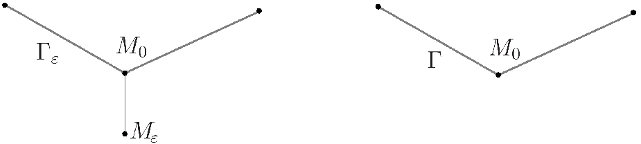
In order to demonstrate the difference between our convergence result and those in [1], [7], we consider a simple model of a star graph with two fixed edges and one small edge of the length ε\varepsilon, which was studied in [6], see Figure 3. On the fixed edges we consider a Schrödinger operator −d2d​x2+V±-\frac{d^{2}}{dx^{2}}+V_{\pm} with some continuous potentials, while on the small edge the operator reads as −d2d​x2+ε−1V0(⋅ε)-\frac{d^{2}}{dx^{2}}+\varepsilon^{-1}V_{0}(\,\cdot\,\varepsilon), where V0∈C⁡[0,1]V_{0}\in C[0,1] is some given function. At the vertex M0M_{0} the Kirchhoff condition is imposed, while the vertex MεM_{\varepsilon} is subject to the Dirichlet or Neumann condition. The limiting operator then is just the same operator on finite edges, while at the vertex M0M_{0} we have the Dirichlet condition if the same is imposed at MεM_{\varepsilon}. But if the vertex MεM_{\varepsilon} is subject to the Neumann condition, then in the limit at M0M_{0} we have a delta-interaction, that is, the Kirchhoff condition with a coupling:

u|e−​(M0)=u|e−​(M0)=:u⁡(M0),u|e−​(M0)+u|e−​(M0)=c​u​(M0),c:=∫01V0​(t)​𝑑t.u\big|_{\mathrm{e}_{-}}(M_{0})=u\big|_{\mathrm{e}_{-}}(M_{0})=:u(M_{0}),\qquad u\big|_{\mathrm{e}_{-}}(M_{0})+u\big|_{\mathrm{e}_{-}}(M_{0})=cu(M_{0}),\qquad c:=\int\limits_{0}^{1}V_{0}(t)\,dt.

As we see, the coupling constant cc is determined solely by the potential V0V_{0}.

It is also interesting to compare our Condition (A) with similar conditions in [1] and [7]. All these conditions are close but there are some differences. In our terms, roughly speaking, Non-resonance condition 3.2 in [1] says that there are no embedded eigenvalues at the bottom of the essential spectrum for all ε>0\varepsilon>0. Namely, we should repeat the rescaling we employed while obtaining the operator ℋ∞\mathcal{H}_{\infty} in (2.8), (2.11) but without letting ε=0\varepsilon=0. This gives an operator depending on ε\varepsilon and coinciding with ℋ∞\mathcal{H}_{\infty} as ε=0\varepsilon=0. Such operator can not have an embedded eigenvalue at the bottom of its essential spectrum for ε>0\varepsilon>0. This does not imply that the same holds for ε=0\varepsilon=0 and this is the main difference between our Condition (A) and Non-resonance condition in [1]. Once we make the aforementioned rescaling of small edges for the model studied in [7], we arrive at an operator on the graph γ∞\gamma_{\infty}, which is independent of ε\varepsilon and coincides with our operator ℋ∞\mathcal{H}_{\infty}. In this specific situation, in [7], there were considered two cases: generic and non-generic ones. The generic case corresponds to the absence of embedded eigenvalues. In the non-generic case, there can be both virtual level and embedded eigenvalues at the bottom of the essential spectrum. But since the model in [7] was quite specific, it was possible to study the the convergence of the resolvent in the non-generic case as well.

In the present work we do not study the case when Condition (A) is violated and the operator has an embedded eigenvalue at the bottom of the essential spectrum. The reason is that although our technique is sufficient to treat such case, it involves more technical details. The nature of the expected results also suggests that this case deserves an independent study, which we postpone for the next work.

3.2 Generalizations of model

Here we discuss possible ways of extending our results to more general models.

The first possibility concerns a case, when instead of one graph γε\gamma_{\varepsilon}, several similar small rescaled graphs γε(j)\gamma_{\varepsilon}^{(j)} are glued at different vertices of the graph Γ\Gamma, see Figure 4. Each of the small graphs γε(j)\gamma_{\varepsilon}^{(j)} can be introduced via rescaling by means of an associated small parameter ε(i)\varepsilon^{(i)}; then coefficients pε(j)p_{\varepsilon}^{(j)}, qε(j)q_{\varepsilon}^{(j)}, Vε(j)V_{\varepsilon}^{(j)} of the differential expression on each such graph γε(j)\gamma_{\varepsilon}^{(j)} are still defined by formula (2.2), but now on each graph γε(j)\gamma_{\varepsilon}^{(j)} the rescaling is made by means of a corresponding operator 𝒮ε(j)\mathcal{S}_{\varepsilon}^{(j)}. We can suppose first that all parameters ε(j)\varepsilon^{(j)} are analytic functions in a single small parameter ε\varepsilon. In this situation, all our results remain valid with obvious minor changes; in particular, the form of the limiting vertex condition at a vertex M0(j)M_{0}^{(j)}, to which the graph γε(j)\gamma_{\varepsilon}^{(j)} is attached, is determined only by the graph γε(j)\gamma_{\varepsilon}^{(j)} and there is no influence by the neighbouring ones.
Refer to caption
Figure 3: Star graph with a small edge and the limiting graph without the small edge.

A more general situation is when in the same setting we assume that the parameters ε(j)\varepsilon^{(j)} are independent and all coefficients in the differential expression and vertex conditions of the operator ℋε\mathcal{H}_{\varepsilon} depend analytically in all ε(j)\varepsilon^{(j)}. In such case, we first of all should assume additionally that for each attached graph γε(j)\gamma_{\varepsilon}^{(j)} and each vertex M∈γ∞(j)M\in\gamma_{\infty}^{(j)}, identities similar to (2.9) hold:

ε(j)​E~M​(ε(j))​AM​(ε)=(ε(j))μ​(AM(0)+ε(j)​AM(1))+O⁡(|ε|2+μ),\displaystyle\varepsilon^{(j)}\tilde{\mathrm{E}}_{M}(\varepsilon^{(j)})\mathrm{A}_{M}(\varepsilon)=\big(\varepsilon^{(j)}\big)^{\mu}\big(\mathrm{A}_{M}^{(0)}+\varepsilon^{(j)}\mathrm{A}_{M}^{(1)}\big)+O(|\varepsilon|^{2+\mu}),
E~M​(ε(j))​BM​(ε)=(ε(j))μ​(BM(0)+ε(j)​BM(1))+O⁡(|ε|2+μ),\displaystyle\tilde{\mathrm{E}}_{M}(\varepsilon^{(j)})\mathrm{B}_{M}(\varepsilon)=\big(\varepsilon^{(j)}\big)^{\mu}\big(\mathrm{B}_{M}^{(0)}+\varepsilon^{(j)}\mathrm{B}_{M}^{(1)}\big)+O(|\varepsilon|^{2+\mu}),

where μ=0\mu=0 if BM​(0)≠0\mathrm{B}_{M}(0)\neq 0 and μ=1\mu=1 if BM​(0)=0\mathrm{B}_{M}(0)=0 and ε=(ε(1),ε(2),…)\varepsilon=(\varepsilon^{(1)},\varepsilon^{(2)},\ldots). For the coefficients of the differential expression we should assume that

pγ(j)​(⋅,ε)=pγ(j)​(⋅,0)+ε(j)​d​pγ(j)d​ε(j)​(⋅,0)+O⁡(|ε|2),p_{\gamma^{(j)}}(\,\cdot\,,\varepsilon)=p_{\gamma^{(j)}}(\,\cdot\,,0)+\varepsilon^{(j)}\frac{dp_{\gamma^{(j)}}}{d\varepsilon^{(j)}}(\,\cdot\,,0)+O(|\varepsilon|^{2}), (3.4)

and the same should hold for the other coefficients. Then the corresponding matrices Q(j)Q^{(j)} are to be calculated for each graph γ(j)\gamma^{(j)} by formulae (2.23), (2.24), (2.25), (2.26). If for some jj the matrix Q(j)Q^{(j)} turns out to have a zero eigenvalue, then assumptions (2.9), (3.4) should be replaced by stricter ones:

ε(j)​E~M​(ε(j))​AM​(ε)=(ε(j))μ​(AM(0)+ε(j)​AM(1))+O⁡(|ε|2+μ),\displaystyle\varepsilon^{(j)}\tilde{\mathrm{E}}_{M}(\varepsilon^{(j)})\mathrm{A}_{M}(\varepsilon)=\big(\varepsilon^{(j)}\big)^{\mu}\big(\mathrm{A}_{M}^{(0)}+\varepsilon^{(j)}\mathrm{A}_{M}^{(1)}\big)+O(|\varepsilon|^{2+\mu}),
E~M​(ε(j))​BM​(ε)=(ε(j))μ​(BM(0)+ε(j)​BM(1))+O⁡(|ε|2+μ),\displaystyle\tilde{\mathrm{E}}_{M}(\varepsilon^{(j)})\mathrm{B}_{M}(\varepsilon)=\big(\varepsilon^{(j)}\big)^{\mu}\big(\mathrm{B}_{M}^{(0)}+\varepsilon^{(j)}\mathrm{B}_{M}^{(1)}\big)+O(|\varepsilon|^{2+\mu}),
pγ(j)​(⋅,ε)=pγ(j)​(⋅,0)+ε(j)​d​pγ(j)d​ε(j)​(⋅,0)+(ε(j))22​d2​pγ(j)d​(ε(j))2​(⋅,0)+O⁡(|ε|3).\displaystyle p_{\gamma^{(j)}}(\,\cdot\,,\varepsilon)=p_{\gamma^{(j)}}(\,\cdot\,,0)+\varepsilon^{(j)}\frac{dp_{\gamma^{(j)}}}{d\varepsilon^{(j)}}(\,\cdot\,,0)+\frac{\big(\varepsilon^{(j)}\big)^{2}}{2}\frac{d^{2}p_{\gamma^{(j)}}}{d(\varepsilon^{(j)})^{2}}(\,\cdot\,,0)+O(|\varepsilon|^{3}).

The above conditions mean that the coefficients in the differential expression and vertex conditions can depend on all small parameters, but the leading terms in their Taylor should be as specified above. Under such assumptions, all our results remain true and now the analyticity holds with respect to all parameters ε(i)\varepsilon^{(i)}. Once these assumptions fail, in the general situation, the result on analyticity is no longer valid. The reason for this situation is in fact a well-known phenomenon in the multi-parametric perturbation theory, which says that the eigenvalues of a matrix analytic with respect to more than one small parameter are not necessary analytic, see [11, Ch. I​I, Sect. 5.7]. The same also concerns the case, when several graphs γ(j)\gamma^{(j)} are rescaled by means of different independent small parameters and are glued to the same vertex in the graph Γ\Gamma. In such general situation one can expect only a convergence result as one proved in [1]. Of course, this does not exclude the situations, when for some particular graphs and specific choices of small edges, differential expression and vertex conditions, the resolvent has the analyticity property, but this can happen only due to some specific features of the considered models.

Refer to caption
Figure 4: Graph Γ\Gamma with several glued small graphs

One more important way of extending our model is to assume that all coefficients in the differential expression and the vertex conditions are not analytic in ε\varepsilon but either infinite differentiable or just possess power asymptotic expansions in ε\varepsilon. In these cases all our results, including ones just discussed above for several glued small graphs, remain true with appropriate modifications. Namely, if the mentioned coefficients are infinite differentiable in ε\varepsilon, then the statement on the analyticity property is to be replaced by the infinite differentiability in ε\varepsilon for the operators ℛΓ\mathcal{R}_{\Gamma} and ℛγ\mathcal{R}_{\gamma}. If the coefficients in the differential expression and the vertex conditions just possess power asymptotic expansions in ε\varepsilon, then the operators ℛΓ\mathcal{R}_{\Gamma} and ℛγ\mathcal{R}_{\gamma} also have power asymptotic expansions in ε\varepsilon. The way of proving such results is very simple and is based on the analyticity case treated above. Namely, we represent the matrices in the vertex conditions as

AM​(ε)=AM(0)+ε​AM(1)+ε2​AM(2)+ε3​A˘M​(ε),BM​(ε)=BM(0)+ε​BM(1)+ε2​BM(2)+ε3​B˘M​(ε),\mathrm{A}_{M}(\varepsilon)=\mathrm{A}_{M}^{(0)}+\varepsilon\mathrm{A}_{M}^{(1)}+\varepsilon^{2}\mathrm{A}_{M}^{(2)}+\varepsilon^{3}\breve{\mathrm{A}}_{M}(\varepsilon),\qquad\mathrm{B}_{M}(\varepsilon)=\mathrm{B}_{M}^{(0)}+\varepsilon\mathrm{B}_{M}^{(1)}+\varepsilon^{2}\mathrm{B}_{M}^{(2)}+\varepsilon^{3}\breve{\mathrm{B}}_{M}(\varepsilon), (3.5)

where the matrices A˘M​(ε)\breve{\mathrm{A}}_{M}(\varepsilon) and B˘M​(ε)\breve{\mathrm{B}}_{M}(\varepsilon) are either infinitely differentiable in ε\varepsilon or have power in ε\varepsilon asymptotic expansions. For the coefficients of the differentiable expression, a similar representation is to be employed. The terms A˘M\breve{\mathrm{A}}_{M} and B˘M\breve{\mathrm{B}}_{M} are to be treated as frozen coefficients independent of ε\varepsilon and the matrices in (3.5) should be treated as second order polynomials in ε\varepsilon. Then it is possible to track the dependence on A˘M\breve{\mathrm{A}}_{M} and B˘M​(ε)\breve{\mathrm{B}}_{M}(\varepsilon) and on similar terms for the coefficients in the differential expression in the proof of Theorem 2.1. As a result, then one can see that the operators ℛΓ\mathcal{R}_{\Gamma} and ℛγ\mathcal{R}_{\gamma} as well as the resolvent (ℋε−λ)−1(\mathcal{H}_{\varepsilon}-\lambda)^{-1} are represented by convergent series (3.1) and (3.2), but now with coefficients depending on ε\varepsilon. These coefficients are either infinitely differentiable in ε\varepsilon or possess power in ε\varepsilon asymptotic expansions. In the first case we conclude immediately that all the operators in question are infinitely differentiable in ε\varepsilon, while in the other case we can easily find the asymptotic expansions for these operators from their series.

4 Self-adjointness

Our main result includes a statement on the self-adjointness of both perturbed and limiting operators and in the proofs, we shall also use the same property for certain auxiliary operators. In this section we first establish a criterion of the self-adjointness for a general operator. Then we shall employ it to prove the same property for the operators ℋ0\mathcal{H}_{0} and ℋγ\mathcal{H}_{\gamma}.

4.1 Criterion of self-adjointness

Let Ξ\Xi be a finite metric graph having no isolated vertices; the lengths of its edges can be both finite or infinite. On each edge we fix arbitrarily an orientation and as above, by d⁡(M)d(M) we denote the degree of a vertex M∈ΞM\in\Xi.

We consider an unbounded operator ℋ\mathcal{H} in L2​(Ξ)L_{2}(\Xi) with the differential expression

ℋ^​u:=−dd​x​p​d​ud​x+i⁡(dd​x​(q​u)+q​d​ud​x)+V​u\hat{\mathcal{H}}u:=-\frac{d\ }{dx}p\frac{du}{dx}+\mathrm{i}\left(\frac{d\ }{dx}(qu)+q\frac{du}{dx}\right)+Vu

subject to the vertex conditions

AM​𝒰M​(u)+BM​𝒰M′​(u)=0at each vertex M.\mathrm{A}_{M}\mathcal{U}_{M}(u)+\mathrm{B}_{M}\mathcal{U}_{M}^{\prime}(u)=0\quad\text{at each vertex $M$}. (4.1)

Here p,q∈W∞1​(Ξ)p,\,q\in W_{\infty}^{1}(\Xi), V∈L2​(Ξ)V\in L_{2}(\Xi) are real-valued functions, while AM\mathrm{A}_{M} and BM\mathrm{B}_{M} are some matrices of size d⁡(M)×d⁡(M)d(M)\times d(M). The ellipticity condition is assumed: p⩾c>0p\geqslant c>0 uniformly on Ξ\Xi. The domain of the operator ℋ\mathcal{H} consists of the functions in W˙22​(Ξ)\dot{W}_{2}^{2}(\Xi) obeying vertex condition (4.1).

By ΠM\Pi_{M}, ΘM\Theta_{M} we denote the following diagonal matrices with real entries:

ΠM:=diag⁡{νi​(M)​p|ei​(M)​(M,ε)}i=1,…,d⁡(M),ΘM:=diag⁡{νi​(M)​q|ei​(M)​(M,ε)}i=1,…,d⁡(M),\Pi_{M}:=\diag\big\{\nu_{i}(M)p\big|_{\mathrm{e}_{i}(M)}(M,\varepsilon)\big\}_{i=1,\ldots,d(M)},\qquad\Theta_{M}:=\diag\big\{\nu_{i}(M)q\big|_{\mathrm{e}_{i}(M)}(M,\varepsilon)\big\}_{i=1,\ldots,d(M)},

where ei​(M)\mathrm{e}_{i}(M) are the edges incident to the vertex MM and the numbers νi​(M)\nu_{i}(M) are defined in the same way as in (2.6).

The main statement of this subsection is the following lemma.

Lemma 4.1.

The operator ℋ\mathcal{H} is self-adjoint if and only if for each vertex M∈ΞM\in\Xi the matrices AM\mathrm{A}_{M} and BM\mathrm{B}_{M} satisfy the rank condition

rank⁡(AM​BM)=d⁡(M)\rank(\mathrm{A}_{M}\ \mathrm{B}_{M})=d(M) (4.2)

and the matrix

AM​ΠM−1​BM∗+iBM​ΠM−1​ΘM​ΠM−1​BM∗\mathrm{A}_{M}\Pi_{M}^{-1}\mathrm{B}_{M}^{*}+\mathrm{i}\mathrm{B}_{M}\Pi_{M}^{-1}\Theta_{M}\Pi_{M}^{-1}\mathrm{B}_{M}^{*} (4.3)

is self-adjoint. Under these restrictions, vertex condition (4.1) can be equivalently rewritten as

i⁡(UM−Id⁡(M))​𝒰M​(u)+(UM+Id⁡(M))​(ΠM​𝒰M′​(u)−i​ΘM​𝒰M​(u))=0,\mathrm{i}(\mathrm{U}_{M}-\mathrm{I}_{d(M)})\mathcal{U}_{M}(u)+(\mathrm{U}_{M}+\mathrm{I}_{d(M)})\big(\Pi_{M}\mathcal{U}_{M}^{\prime}(u)-\mathrm{i}\Theta_{M}\mathcal{U}_{M}(u)\big)=0, (4.4)

where the matrix

UM:=−(AM+iBM​ΠM−1​(ΘM−Id⁡(M)))−1​(AM+iBM​ΠM−1​(ΘM+Id⁡(M)))\mathrm{U}_{M}:=-\big(\mathrm{A}_{M}+\mathrm{i}\mathrm{B}_{M}\Pi_{M}^{-1}(\Theta_{M}-\mathrm{I}_{d(M)})\big)^{-1}\big(\mathrm{A}_{M}+\mathrm{i}\mathrm{B}_{M}\Pi_{M}^{-1}(\Theta_{M}+\mathrm{I}_{d(M)})\big)

is well-defined and is unitary.

Proof.

In a particular case p≡1p\equiv 1, q≡0q\equiv 0, V≡0V\equiv 0, the lemma states a well-known result, see Theorem 1.1.4 in [2, Ch. 1, Sect. 1.4.]. In fact, the proof of this theorem can be adapted also for our more general case up to some minor changes. Below we describe how to do this.

First of all we observe that vertex condition (4.1) can be equivalently rewritten as

A~M​𝒰M​(u)+B~M​(ΠM​𝒰M′​(u)−i​ΘM​𝒰M​(u))=0,\displaystyle\tilde{\mathrm{A}}_{M}\mathcal{U}_{M}(u)+\tilde{\mathrm{B}}_{M}\big(\Pi_{M}\mathcal{U}_{M}^{\prime}(u)-\mathrm{i}\Theta_{M}\mathcal{U}_{M}(u)\big)=0, (4.5)
A~M:=AM+iBM​ΠM−1​ΘM,B~M:=BM​ΠM−1.\displaystyle\tilde{\mathrm{A}}_{M}:=\mathrm{A}_{M}+\mathrm{i}\mathrm{B}_{M}\Pi_{M}^{-1}\Theta_{M},\qquad\tilde{\mathrm{B}}_{M}:=\mathrm{B}_{M}\Pi_{M}^{-1}. (4.6)

Let uu be an arbitrary function from the domain of the operator ℋ\mathcal{H} and vv be an arbitrary function from ⨁e∈ΞC∞​(e)\bigoplus\limits_{\mathrm{e}\in\Xi}C^{\infty}(\mathrm{e}) vanishing outside a small neighbourhood of an arbitrarily fixed vertex M∈ΞM\in\Xi. Integrating twice by parts, we get:

(ℋ​u,v)L2​(Ξ)=\displaystyle(\mathcal{H}u,v)_{L_{2}(\Xi)}= (ΠM​𝒰M′​(u),𝒰M​(v))ℂd⁡(M)−(𝒰M​(u),ΠM​𝒰M′​(v))ℂd⁡(M)+(u,ℋ^​v)L2​(Ξ)\displaystyle\big(\Pi_{M}\mathcal{U}_{M}^{\prime}(u),\mathcal{U}_{M}(v)\big)_{\mathds{C}^{d(M)}}-\big(\mathcal{U}_{M}(u),\Pi_{M}\mathcal{U}_{M}^{\prime}(v)\big)_{\mathds{C}^{d(M)}}+(u,\hat{\mathcal{H}}v)_{L_{2}(\Xi)}
=\displaystyle= (𝖥M′,𝖦M)ℂd⁡(M)−(𝖥M,𝖦M′)ℂd⁡(M)+(u,ℋ^​v)L2​(Ξ),\displaystyle(\mathsf{F}_{M}^{\prime},\mathsf{G}_{M})_{\mathds{C}^{d(M)}}-(\mathsf{F}_{M},\mathsf{G}_{M}^{\prime})_{\mathds{C}^{d(M)}}+(u,\hat{\mathcal{H}}v)_{L_{2}(\Xi)},

where

𝖥M′:=ΠM​𝒰M′​(u)−i​ΘM​𝒰M​(u),𝖦M:=𝒰M​(v),\displaystyle\mathsf{F}_{M}^{\prime}:=\Pi_{M}\mathcal{U}_{M}^{\prime}(u)-\mathrm{i}\Theta_{M}\mathcal{U}_{M}(u),\qquad\mathsf{G}_{M}:=\mathcal{U}_{M}(v),
𝖥M:=𝒰M​(u),𝖦M′:=ΠM​𝒰M′​(v)−i​ΘM​𝒰M​(v).\displaystyle\mathsf{F}_{M}:=\mathcal{U}_{M}(u),\qquad\mathsf{G}_{M}^{\prime}:=\Pi_{M}\mathcal{U}_{M}^{\prime}(v)-\mathrm{i}\Theta_{M}\mathcal{U}_{M}(v).

Hence, the function vv is in the domain of the adjoint operator ℋ∗\mathcal{H}^{*} if

(𝖥M′,𝖦M)ℂd⁡(M)−(𝖥M,𝖦M′)ℂd⁡(M)=0.(\mathsf{F}_{M}^{\prime},\mathsf{G}_{M})_{\mathds{C}^{d(M)}}-(\mathsf{F}_{M},\mathsf{G}_{M}^{\prime})_{\mathds{C}^{d(M)}}=0.

The latter identity is exactly equation (1.4.16) in the proof of Theorem 1.1.4 in [2, Ch. 1, Sect. 1.4] but with different 𝖥M\mathsf{F}_{M}, 𝖥M′\mathsf{F}_{M}^{\prime}, 𝖦M\mathsf{G}_{M}, 𝖦M′\mathsf{G}_{M}^{\prime}. However, the specific form of these quantities were not important in that proof in [2]. This is why the arguing from [2] can be reproduced literally with above introduced 𝖥M\mathsf{F}_{M}, 𝖥M′\mathsf{F}_{M}^{\prime}, 𝖦M\mathsf{G}_{M}, 𝖦M′\mathsf{G}_{M}^{\prime}; as the matrices AA and BB used in that proof, our matrices A~M\tilde{\mathrm{A}}_{M} and B~M\tilde{\mathrm{B}}_{M} serve. Rank condition (4.2) is equivalent to similar condition (1.4.10) in [2, Ch. 1, Sect. 1.4] since thanks to the non-degeneracy of the matrix ΠM−1\Pi_{M}^{-1} we have

rank⁡(A~M​B~M)=\displaystyle\rank(\tilde{\mathrm{A}}_{M}\ \;\tilde{\mathrm{B}}_{M})= rank⁡(AM+iBM​ΠM−1​ΘM​BM​ΠM−1)\displaystyle\rank\big(\mathrm{A}_{M}+\mathrm{i}\mathrm{B}_{M}\Pi_{M}^{-1}\Theta_{M}\ \;\mathrm{B}_{M}\Pi_{M}^{-1}\big)
=\displaystyle= rank⁡(AM​BM​ΠM−1)=rank⁡(AM​BM)=d⁡(M).\displaystyle\rank\big(\mathrm{A}_{M}\ \;\mathrm{B}_{M}\Pi_{M}^{-1}\big)=\rank\big(\mathrm{A}_{M}\ \;\mathrm{B}_{M}\big)=d(M).

Condition (1.4.11) for the matrices AA and BB from Theorem 1.1.4 in [2, Ch. 1, Sect. 1.4.] is exactly our condition (4.3), while equivalent formulation (4.4) of the vertex condition are implied immediately by similar formulations (1.4.13) in [2]. The proof is complete. ∎

4.2 Self-adjointness of operators ℋ0\mathcal{H}_{0} and ℋ∞\mathcal{H}_{\infty}

In this subsection we prove that under the assumptions of Theorem 2.1 the operators ℋ0\mathcal{H}_{0} and ℋ∞\mathcal{H}_{\infty} are self-adjoint. In order to prove this statement for the operator ℋ0\mathcal{H}_{0}, we shall need the self-adjointness of the matrix Q\mathrm{Q} involved in the matrix AM0(0)\mathrm{A}_{M_{0}}^{(0)}, see (2.22). This fact is provided by the following lemma, which will be independently proved later in a separate subsection, see Subsection 4.3.

Lemma 4.2.

The matrix Q\mathrm{Q} is self-adjoint.

Let us show that the operators ℋ0\mathcal{H}_{0} and ℋ∞\mathcal{H}_{\infty} are self-adjoint. The matrix in (2.5) is self-adjoint as ε=0\varepsilon=0 for each vertex M∈ΓM\in\Gamma, M≠M0M\neq M_{0}. Hence, the matrices AM(0)\mathrm{A}_{M}^{(0)}, BM(0)\mathrm{B}_{M}^{(0)} satisfy condition (4.2), (4.3) for each vertex M∈ΓM\in\Gamma, M≠M0M\neq M_{0}. Thanks to the self-adjointness of the matrix Q\mathrm{Q} stated in Lemma 4.2, the self-adjointness of the matrix in (4.3) corresponding to the matrices AM0(0)\mathrm{A}_{M_{0}}^{(0)} and BM0(0)\mathrm{B}_{M_{0}}^{(0)} is confirmed by simple straightforward calculations. In view of the non-degeneracy of the matrix ΠΓ,M0​(0)\Pi_{\Gamma,M_{0}}(0), condition (4.2) corresponding to the same matrices is checked as follows:

rank⁡(AM0(0)​BM0(0))=\displaystyle\rank\big(\mathrm{A}_{M_{0}}^{(0)}\ \mathrm{B}_{M_{0}}^{(0)}\big)= rank⁡(AM0(0)+iBM0(0)​ΠΓ,M0−1​(0)​ΘΓ,M0​(0)​Ψ−BM0(0)​ΠΓ,M0−1​(0)​Ψ)\displaystyle\rank\Big(\mathrm{A}_{M_{0}}^{(0)}+\mathrm{i}\mathrm{B}_{M_{0}}^{(0)}\Pi_{\Gamma,M_{0}}^{-1}(0)\Theta_{\Gamma,M_{0}}(0)\Psi\quad-\mathrm{B}_{M_{0}}^{(0)}\Pi_{\Gamma,M_{0}}^{-1}(0)\Psi\Big)
=\displaystyle= rank⁡((Q00Id0−k)(Ik000))=d0.\displaystyle\rank\left(\begin{pmatrix}\mathrm{Q}&0\\ 0&\mathrm{I}_{d_{0}-k}\end{pmatrix}\quad\begin{pmatrix}\mathrm{I}_{k}&0\\ 0&0\end{pmatrix}\right)=d_{0}.

Hence, we can apply Lemma 4.1 and we see that the operator ℋ0\mathcal{H}_{0} is self-adjoint.

We proceed to proving the self-adjointness of the operator ℋ∞\mathcal{H}_{\infty}. In view of the assumption on the matrices AM​(0)\mathrm{A}_{M}(0) and BM​(0)\mathrm{B}_{M}(0) made in Subsection 2.1, see the explanation after (2.4), we see easily that rank condition (2.7) implies the same for the matrices AM(0)\mathrm{A}_{M}^{(0)} and BM(0)\mathrm{B}_{M}^{(0)} defined in (2.10). Then we multiply the matrix in (2.5) by ε\varepsilon and then by E~M​(ε)\tilde{\mathrm{E}}_{M}(\varepsilon) from left and right keeping its self-adjointness and then we pass to the limit as ε→+0\varepsilon\to+0. By identities (2.9) we then arrive to the self-adjointness of the matrix

AM(0)​Πγ,M−1​(0)​(BM(0))∗+iBM(0)​Πγ,M−1​(0)​Θγ,M​(0)​Πγ,M−1​(0)​(BM(0))∗.\mathrm{A}_{M}^{(0)}\Pi_{\gamma,M}^{-1}(0)\big(\mathrm{B}_{M}^{(0)}\big)^{*}+\mathrm{i}\mathrm{B}_{M}^{(0)}\Pi_{\gamma,M}^{-1}(0)\Theta_{\gamma,M}(0)\Pi_{\gamma,M}^{-1}(0)\big(\mathrm{B}_{M}^{(0)}\big)^{*}.

Applying now Lemma 4.1, we conclude that the operator ℋ∞\mathcal{H}_{\infty} is self-adjoint.

4.3 Self-adjointness of Q\mathrm{Q}

In this section we prove Lemma 4.2. The proof is based on obtaining certain representations for the operators ℒM\mathcal{L}_{M} and ℰM\mathcal{E}_{M} used in (2.25), (2.26), (2.27), which will imply then the desired self-adjointness. These representations are based on an appropriate transformation of vertex conditions (2.4) at M∈γεM\in\gamma_{\varepsilon} and we begin our proof with describing them.

Given a vertex M∈γεM\in\gamma_{\varepsilon}, including vertices M=MjM=M_{j}, j=1,…,nj=1,\ldots,n, we rescale the variables as ξ=x​ε−1\xi=x\varepsilon^{-1} passing in fact to the graph γ∞\gamma_{\infty}. Then vertex condition (2.4) becomes

ε​AM​(ε)​𝒰M​(u)+BM​(ε)​𝒰M′​(u)=0,\varepsilon\mathrm{A}_{M}(\varepsilon)\mathcal{U}_{M}(u)+\mathrm{B}_{M}(\varepsilon)\mathcal{U}_{M}^{\prime}(u)=0, (4.7)

where the vectors 𝒰M​(u)\mathcal{U}_{M}(u) and 𝒰M′​(u)\mathcal{U}_{M}^{\prime}(u) are introduced as above but are treated in terms of the variable ξ\xi. According Lemma 4.1, at each vertex M∈γ∞M\in\gamma_{\infty} the above vertex condition can be equivalently rewritten as

i⁡(UM​(ε)−Id⁡(M))​𝒰M​(u)+(UM​(ε)+Id⁡(M))​(Πγ,M​(ε)​𝒰M′​(u)−i​Θγ,M​(ε)​𝒰M​(u))=0,\mathrm{i}(\mathrm{U}_{M}(\varepsilon)-\mathrm{I}_{d(M)})\mathcal{U}_{M}(u)+(\mathrm{U}_{M}(\varepsilon)+\mathrm{I}_{d(M)})\big(\Pi_{\gamma,M}(\varepsilon)\mathcal{U}_{M}^{\prime}(u)-\mathrm{i}\Theta_{\gamma,M}(\varepsilon)\mathcal{U}_{M}(u)\big)=0, (4.8)

where, we recall, the matrices Πγ,M\Pi_{\gamma,M} and Θγ,M\Theta_{\gamma,M} were defined in (2.29), and

UM(ε):=−\displaystyle\mathrm{U}_{M}(\varepsilon):=- (ε​AM​(ε)+iBM​(ε)​Πγ,M−1​(ε)​(Θγ,M​M​(ε)−Id⁡(M)))−1\displaystyle\Big(\varepsilon\mathrm{A}_{M}(\varepsilon)+\mathrm{i}\mathrm{B}_{M}(\varepsilon)\Pi_{\gamma,M}^{-1}(\varepsilon)\big(\Theta_{\gamma,M}M(\varepsilon)-\mathrm{I}_{d(M)}\big)\Big)^{-1} (4.9)
⋅(ε​AM​(ε)+iBM​(ε)​Πγ,M−1​(ε)​(Θγ,M​(ε)+Id⁡(M)))\displaystyle\cdot\Big(\varepsilon\mathrm{A}_{M}(\varepsilon)+\mathrm{i}\mathrm{B}_{M}(\varepsilon)\Pi_{\gamma,M}^{-1}(\varepsilon)\big(\Theta_{\gamma,M}(\varepsilon)+\mathrm{I}_{d(M)}\big)\Big)

is an unitary matrix.

Lemma 4.3.

For all M∈ΓM\in\Gamma, M≠M0M\neq M_{0} and all M∈γ∞M\in\gamma_{\infty}, the matrix UM​(ε)\mathrm{U}_{M}(\varepsilon) is analytic in ε\varepsilon.

Proof.

In view of rank condition (2.7) and formulae (2.9) and owing to the analyticity of AM​(ε)\mathrm{A}_{M}(\varepsilon) and BM​(ε)\mathrm{B}_{M}(\varepsilon) in ε\varepsilon, the matrix UM​(ε)\mathrm{U}_{M}(\varepsilon) is meromorphic in ε\varepsilon. At the same time, by the unitarity of UM​(ε)\mathrm{U}_{M}(\varepsilon) we have ‖UM​(ε)​x‖ℂd⁡(M)=‖x‖ℂd⁡(M)\|\mathrm{U}_{M}(\varepsilon)\mathrm{x}\|_{\mathds{C}^{d(M)}}=\|\mathrm{x}\|_{\mathds{C}^{d(M)}} for all x∈ℂd⁡(M)\mathrm{x}\in\mathds{C}^{d(M)} and sufficiently small ε\varepsilon. Hence, the matrix UM​(ε)\mathrm{U}_{M}(\varepsilon) is bounded uniformly in ε\varepsilon and can not have poles. Therefore, it is analytic in ε\varepsilon. The proof is complete. ∎

Thanks to the unitarity of the matrix UM​(ε)\mathrm{U}_{M}(\varepsilon), by the results in [11, Ch. I​I, Sec. 4.6], the eigenvalues and the associated orthonormalized in ℂd⁡(M)\mathds{C}^{d(M)} vectors of the matrix UM​(ε)\mathrm{U}_{M}(\varepsilon) are analytic in ε\varepsilon. By PM​(ε)\mathrm{P}_{M}(\varepsilon) we denote the total projector in ℂd⁡(M)\mathds{C}^{d(M)} onto the eigenspace associated with the eigenvalues of the matrix UM​(ε)\mathrm{U}_{M}(\varepsilon) converging to −1-1 as ε→+0\varepsilon\to+0. We also let PM,⊥​(ε):=Id⁡(M)−PM​(ε)\mathrm{P}_{M,\bot}(\varepsilon):=\mathrm{I}_{d(M)}-\mathrm{P}_{M}(\varepsilon). By the aforementioned analyticity in ε\varepsilon of the eigenvalues and the eigenvectors of UM​(ε)\mathrm{U}_{M}(\varepsilon), the projectors PM​(ε)\mathrm{P}_{M}(\varepsilon) and PM,⊥​(ε)\mathrm{P}_{M,\bot}(\varepsilon) are also analytic in ε\varepsilon.

We apply the projectors PM​(ε)\mathrm{P}_{M}(\varepsilon) and PM,⊥​(ε)\mathrm{P}_{M,\bot}(\varepsilon) to vertex condition (4.8) and we rewrite it equivalently as

PM​(ε)​𝒰M​(u)+KM​(ε)​(Πγ,M​(ε)​𝒰M′​(u)−i​Θγ,M​(ε)​𝒰M​(u))=0,\displaystyle\mathrm{P}_{M}(\varepsilon)\mathcal{U}_{M}(u)+\mathrm{K}_{M}(\varepsilon)\big(\Pi_{\gamma,M}(\varepsilon)\mathcal{U}_{M}^{\prime}(u)-\mathrm{i}\Theta_{\gamma,M}(\varepsilon)\mathcal{U}_{M}(u)\big)=0, (4.10)
PM,⊥​(ε)​Πγ,M​(ε)​𝒰M′​(u)+(KM,⊥​(ε)−iPM,⊥​(ε)​Θγ,M​(ε))​𝒰M​(u)=0,\displaystyle\mathrm{P}_{M,\bot}(\varepsilon)\Pi_{\gamma,M}(\varepsilon)\mathcal{U}_{M}^{\prime}(u)+\big(\mathrm{K}_{M,\bot}(\varepsilon)-\mathrm{i}\mathrm{P}_{M,\bot}(\varepsilon)\Theta_{\gamma,M}(\varepsilon)\big)\mathcal{U}_{M}(u)=0,

where

KM​(ε):=−i​(UM​(ε)−Id⁡(M))−1​PM​(ε)​(UM​(ε)+Id⁡(M))\displaystyle\mathrm{K}_{M}(\varepsilon):=-\mathrm{i}\big(\mathrm{U}_{M}(\varepsilon)-\mathrm{I}_{d(M)}\big)^{-1}\mathrm{P}_{M}(\varepsilon)\big(\mathrm{U}_{M}(\varepsilon)+\mathrm{I}_{d(M)}\big) (4.11)
KM,⊥​(ε):=i​(UM​(ε)+Id⁡(M))−1​PM,⊥​(ε)​(UM​(ε)−Id⁡(M)).\displaystyle\mathrm{K}_{M,\bot}(\varepsilon):=\mathrm{i}\big(\mathrm{U}_{M}(\varepsilon)+\mathrm{I}_{d(M)}\big)^{-1}\mathrm{P}_{M,\bot}(\varepsilon)\big(\mathrm{U}_{M}(\varepsilon)-\mathrm{I}_{d(M)}\big).

It is obvious that both matrices KM​(ε)\mathrm{K}_{M}(\varepsilon) and KM,⊥​(ε)\mathrm{K}_{M,\bot}(\varepsilon) are well-defined and analytic in ε\varepsilon. Employing the unitarity of the matrix UM​(ε)\mathrm{U}_{M}(\varepsilon), it is straightforward to confirm that both matrices KM​(ε)\mathrm{K}_{M}(\varepsilon) and KM,⊥​(ε)\mathrm{K}_{M,\bot}(\varepsilon) are self-adjoint. We also observe that

UM​(0)=UM(0),PM​(0)=PM(0),KM​(0)=0.\mathrm{U}_{M}(0)=\mathrm{U}_{M}^{(0)},\qquad\mathrm{P}_{M}(0)=\mathrm{P}_{M}^{(0)},\qquad\mathrm{K}_{M}(0)=0.

Since the operator PM​(ε)\mathrm{P}_{M}(\varepsilon) is analytic in ε\varepsilon, by the results in [11, Ch. 2, Sect. 4.2], there exists a transforming function for this projector, namely, an invertible operator SM​(ε)\mathrm{S}_{M}(\varepsilon) in ℂd⁡(M)\mathds{C}^{d(M)}, analytic in small ε\varepsilon together with its inverse operator such that

SM​(0)=Id⁡(M),SM−1​(ε)​PM(0)​SM​(ε)=PM​(ε),SM−1​(ε)​PM,⊥(0)​SM​(ε)=PM,⊥​(ε)\mathrm{S}_{M}(0)=\mathrm{I}_{d(M)},\qquad\mathrm{S}_{M}^{-1}(\varepsilon)\mathrm{P}_{M}^{(0)}\mathrm{S}_{M}(\varepsilon)=\mathrm{P}_{M}(\varepsilon),\qquad\mathrm{S}_{M}^{-1}(\varepsilon)\mathrm{P}_{M,\bot}^{(0)}\mathrm{S}_{M}(\varepsilon)=\mathrm{P}_{M,\bot}(\varepsilon) (4.12)

The inverse operator SM−1​(ε)\mathrm{S}_{M}^{-1}(\varepsilon) is given explicitly by formula (4.18) in [11, Ch. 2, Sect. 4.2] and this implies

SM​(ε)=(PM​(ε)​PM(0)+PM,⊥​(ε)​PM,⊥(0))−1​(Id⁡(M)−(PM​(ε)−PM(0))2)12.\mathrm{S}_{M}(\varepsilon)=\big(\mathrm{P}_{M}(\varepsilon)\mathrm{P}_{M}^{(0)}+\mathrm{P}_{M,\bot}(\varepsilon)\mathrm{P}_{M,\bot}^{(0)}\big)^{-1}\Big(\mathrm{I}_{d(M)}-\big(\mathrm{P}_{M}(\varepsilon)-\mathrm{P}_{M}^{(0)}\big)^{2}\Big)^{\frac{1}{2}}. (4.13)

In view of formulae (4.12), (4.13), vertex condition (4.10) can be equivalently rewritten as

PM(0)​SM​(ε)​𝒰M​(u)+SM​(ε)​KM​(ε)​(Πγ,M​(ε)​UM′​(ε)−i​Θγ,M​(ε)​𝒰M​(u))=0,\displaystyle\mathrm{P}_{M}^{(0)}\mathrm{S}_{M}(\varepsilon)\mathcal{U}_{M}(u)+\mathrm{S}_{M}(\varepsilon)\mathrm{K}_{M}(\varepsilon)\big(\Pi_{\gamma,M}(\varepsilon)\mathrm{U}_{M}^{\prime}(\varepsilon)-\mathrm{i}\Theta_{\gamma,M}(\varepsilon)\mathcal{U}_{M}(u)\big)=0,
PM,⊥(0)​SM​(ε)​Πγ,M​M​(ε)​𝒰M′​(u)+SM​(ε)​(KM,⊥​(ε)−iPM,⊥​(ε)​Θγ,M​(ε))​𝒰M​(u)=0.\displaystyle\mathrm{P}_{M,\bot}^{(0)}\mathrm{S}_{M}(\varepsilon)\Pi_{\gamma,M}M(\varepsilon)\mathcal{U}_{M}^{\prime}(u)+\mathrm{S}_{M}(\varepsilon)\big(\mathrm{K}_{M,\bot}(\varepsilon)-\mathrm{i}\mathrm{P}_{M,\bot}(\varepsilon)\Theta_{\gamma,M}(\varepsilon)\big)\mathcal{U}_{M}(u)=0.

Since the first terms in the above identities belong respectively to the spaces PM(0)​ℂd⁡(M)\mathrm{P}_{M}^{(0)}\mathds{C}^{d(M)} and PM,⊥(0)​ℂd⁡(M)\mathrm{P}_{M,\bot}^{(0)}\mathds{C}^{d(M)}, the same is true for the other terms in these identities. Therefore, we can apply the projector PM,⊥(0)\mathrm{P}_{M,\bot}^{(0)} to these identities and we equivalently rewrite them as

PM(0)​S~M​(ε)​𝒰M​(u)+K~M​(ε)​𝒰M′​(u)=0,PM,⊥(0)​S~M,⊥​(ε)​𝒰M′​(u)+K~M,⊥​(ε)​𝒰M​(u)=0,\mathrm{P}_{M}^{(0)}\tilde{\mathrm{S}}_{M}(\varepsilon)\mathcal{U}_{M}(u)+\tilde{\mathrm{K}}_{M}(\varepsilon)\mathcal{U}_{M}^{\prime}(u)=0,\qquad\mathrm{P}_{M,\bot}^{(0)}\tilde{\mathrm{S}}_{M,\bot}(\varepsilon)\mathcal{U}_{M}^{\prime}(u)+\tilde{\mathrm{K}}_{M,\bot}(\varepsilon)\mathcal{U}_{M}(u)=0, (4.14)

where

S~M(ε):=SM(ε)(Id⁡(M)−iKM(ε)Θγ,M(ε)),K~M(ε):=PM(0)SM(ε)KM(ε)Πγ,M(ε),\displaystyle\tilde{\mathrm{S}}_{M}(\varepsilon):=\mathrm{S}_{M}(\varepsilon)\big(\mathrm{I}_{d(M)}-\mathrm{i}\mathrm{K}_{M}(\varepsilon)\Theta_{\gamma,M}(\varepsilon)\big),\qquad\tilde{\mathrm{K}}_{M}(\varepsilon):=\mathrm{P}_{M}^{(0)}\mathrm{S}_{M}(\varepsilon)\mathrm{K}_{M}(\varepsilon)\Pi_{\gamma,M}(\varepsilon), (4.15)
S~M,⊥(ε):=SM(ε)Πγ,M(ε),K~M,⊥(ε):=PM,⊥(0)SM(ε)(KM,⊥(ε)−iPM,⊥(ε)Θγ,M(ε)).\displaystyle\tilde{\mathrm{S}}_{M,\bot}(\varepsilon):=\mathrm{S}_{M}(\varepsilon)\Pi_{\gamma,M}(\varepsilon),\qquad\tilde{\mathrm{K}}_{M,\bot}(\varepsilon):=\mathrm{P}_{M,\bot}^{(0)}\mathrm{S}_{M}(\varepsilon)\big(\mathrm{K}_{M,\bot}(\varepsilon)-\mathrm{i}\mathrm{P}_{M,\bot}(\varepsilon)\Theta_{\gamma,M}(\varepsilon)\big).

The matrices SM​(ε)\mathrm{S}_{M}(\varepsilon), S~M​(ε)\tilde{\mathrm{S}}_{M}(\varepsilon), S~M,⊥​(ε)\tilde{\mathrm{S}}_{M,\bot}(\varepsilon), K~M​(ε)\tilde{\mathrm{K}}_{M}(\varepsilon), K~M,⊥​(ε)\tilde{\mathrm{K}}_{M,\bot}(\varepsilon), Πγ,M​(ε)\Pi_{\gamma,M}(\varepsilon), Θγ,M​(ε)\Theta_{\gamma,M}(\varepsilon) are analytic in ε\varepsilon and by SM,1\mathrm{S}_{M,1}, S~M,1\tilde{\mathrm{S}}_{M,1}, S~M,⊥,1\tilde{\mathrm{S}}_{M,\bot,1}, K~M,1\tilde{\mathrm{K}}_{M,1}, K~M,⊥,1\tilde{\mathrm{K}}_{M,\bot,1}, Πγ,M,1​(ε)\Pi_{\gamma,M,1}(\varepsilon), Θγ,M,1​(ε)\Theta_{\gamma,M,1}(\varepsilon) we denote their derivatives in ε\varepsilon taken at ε=0\varepsilon=0. For instance,

S~M,1:=d​S~Md​ε​(0),S~M,⊥,1:=d​S~M,⊥d​ε​(0).\tilde{S}_{M,1}:=\frac{d\tilde{\mathrm{S}}_{M}}{d\varepsilon}(0),\qquad\tilde{S}_{M,\bot,1}:=\frac{d\tilde{\mathrm{S}}_{M,\bot}}{d\varepsilon}(0).

In order to prove Lemma 4.2, we shall need several properties of the introduced matrices, which are summarized in the following auxiliary statement.

Lemma 4.4.

For each vertex M∈γ∞M\in\gamma_{\infty}, the identities hold:

PM,⊥(0)PM,1=PM,1PM(0),PM,⊥(0)PM,1PM,⊥(0)=0,PM(0)PM,1=PM,1PM,⊥(0),PM(0)PM,1PM(0)=0,PM,1∗=PM,1,\displaystyle\begin{aligned} &\mathrm{P}_{M,\bot}^{(0)}\mathrm{P}_{M,1}=\mathrm{P}_{M,1}\mathrm{P}_{M}^{(0)},\qquad\mathrm{P}_{M,\bot}^{(0)}\mathrm{P}_{M,1}\mathrm{P}_{M,\bot}^{(0)}=0,\\ &\mathrm{P}_{M}^{(0)}\mathrm{P}_{M,1}=\mathrm{P}_{M,1}\mathrm{P}_{M,\bot}^{(0)},\qquad\mathrm{P}_{M}^{(0)}\mathrm{P}_{M,1}\mathrm{P}_{M}^{(0)}=0,\qquad\mathrm{P}_{M,1}^{*}=\mathrm{P}_{M,1},\end{aligned} (4.16)
SM,1=PM,1​PM,⊥(0)−PM,1​PM(0)=PM,1​PM,⊥(0)−PM,⊥(0)​PM,1,\displaystyle\begin{aligned} \mathrm{S}_{M,1}=\mathrm{P}_{M,1}\mathrm{P}_{M,\bot}^{(0)}-\mathrm{P}_{M,1}\mathrm{P}_{M}^{(0)}=\mathrm{P}_{M,1}\mathrm{P}_{M,\bot}^{(0)}-\mathrm{P}_{M,\bot}^{(0)}\mathrm{P}_{M,1},\end{aligned} (4.17)
PM(0)​KM,1​PM,1(0)=0.\displaystyle\mathrm{P}_{M}^{(0)}\mathrm{K}_{M,1}\mathrm{P}_{M,1}^{(0)}=0. (4.18)
Proof.

Formulae (4.16) are obtained immediately via calculating the coefficients at ε1\varepsilon^{1} in the obvious identities:

(PM,⊥​(ε))2=PM,⊥​(ε),(PM​(ε))2=PM​(ε),(PM,⊥​(ε))∗=PM,⊥​(ε).\big(\mathrm{P}_{M,\bot}(\varepsilon)\big)^{2}=\mathrm{P}_{M,\bot}(\varepsilon),\qquad\big(\mathrm{P}_{M}(\varepsilon)\big)^{2}=\mathrm{P}_{M}(\varepsilon),\qquad\big(\mathrm{P}_{M,\bot}(\varepsilon)\big)^{*}=\mathrm{P}_{M,\bot}(\varepsilon).

Formula (4.17) can be confirmed by expanding the right hand side in (4.13) into the power series in ε\varepsilon, calculating the coefficient at ε1\varepsilon^{1}, and employing then (4.16). It follows from the formula for KM​(ε)\mathrm{K}_{M}(\varepsilon) in (4.11) that

i⁡(UM​(ε)−Id⁡(M))​PM​(ε)​KM​(ε)​PM,⊥​(ε)=PM​(ε)​(UM​(ε)+Id⁡(M))​PM,⊥​(ε)=0.\displaystyle\mathrm{i}(\mathrm{U}_{M}(\varepsilon)-\mathrm{I}_{d(M)})\mathrm{P}_{M}(\varepsilon)\mathrm{K}_{M}(\varepsilon)\mathrm{P}_{M,\bot}(\varepsilon)=\mathrm{P}_{M}(\varepsilon)(\mathrm{U}_{M}(\varepsilon)+\mathrm{I}_{d(M)})\mathrm{P}_{M,\bot}(\varepsilon)=0.

Expanding this identity into the power series in ε\varepsilon and calculating the coefficient at ε1\varepsilon^{1}, we arrive at (4.18). The proof is complete. ∎

Now we are in position to prove Lemma 4.2.

Proof of Lemma 4.2.

According definition (4.9) of UM​(ε)\mathrm{U}_{M}(\varepsilon), formulae (4.5), (4.6) applied with

A~M=A~M​(ε):=ε​AM​(ε)+iBM​(ε)​Πγ,M−1​(ε)​Θγ,M​(ε),B~M=B~M​(ε):=BM​(ε)​Πγ,M−1​(ε),\tilde{\mathrm{A}}_{M}=\tilde{\mathrm{A}}_{M}(\varepsilon):=\varepsilon\mathrm{A}_{M}(\varepsilon)+\mathrm{i}\mathrm{B}_{M}(\varepsilon)\Pi_{\gamma,M}^{-1}(\varepsilon)\Theta_{\gamma,M}(\varepsilon),\qquad\tilde{\mathrm{B}}_{M}=\tilde{\mathrm{B}}_{M}(\varepsilon):=\mathrm{B}_{M}(\varepsilon)\Pi_{\gamma,M}^{-1}(\varepsilon),

and the easily checked identities

−2​i​(A~M​(ε)−i​A~M​(ε))−1​A~M​(ε)=i⁡(UM​(ε)−Id⁡(M)),\displaystyle-2\mathrm{i}\big(\tilde{\mathrm{A}}_{M}(\varepsilon)-\mathrm{i}\tilde{\mathrm{A}}_{M}(\varepsilon)\big)^{-1}\tilde{\mathrm{A}}_{M}(\varepsilon)=\mathrm{i}\big(\mathrm{U}_{M}(\varepsilon)-\mathrm{I}_{d(M)}\big),
−2​i​(A~M​(ε)−i​A~M​(ε))−1​B~M​(ε)=UM​(ε)+Id⁡(M),\displaystyle-2\mathrm{i}\big(\tilde{\mathrm{A}}_{M}(\varepsilon)-\mathrm{i}\tilde{\mathrm{A}}_{M}(\varepsilon)\big)^{-1}\tilde{\mathrm{B}}_{M}(\varepsilon)=\mathrm{U}_{M}(\varepsilon)+\mathrm{I}_{d(M)},

for each ψ(i)\psi^{(i)} and each vertex M∈γ∞M\in\gamma_{\infty} we have:

ε​AM​(ε)\displaystyle\varepsilon\mathrm{A}_{M}(\varepsilon) 𝒰M​(ψ(i))+BM​(ε)​𝒰M′​(ψ(i))=i2​(A~M​(ε)−i​B~M​(ε))​(i⁡(UM​(ε)−Id⁡(M))​PM​(ε)CLOSE\displaystyle\mathcal{U}_{M}(\psi^{(i)})+\mathrm{B}_{M}(\varepsilon)\mathcal{U}_{M}^{\prime}(\psi^{(i)})=\frac{\mathrm{i}}{2}\big(\tilde{\mathrm{A}}_{M}(\varepsilon)-\mathrm{i}\tilde{\mathrm{B}}_{M}(\varepsilon)\big)\bigg(\mathrm{i}(\mathrm{U}_{M}(\varepsilon)-\mathrm{I}_{d(M)})\mathrm{P}_{M}(\varepsilon) (4.19)
⋅((Id⁡(M)−iKM​(ε)​Θγ,M​(ε))​𝒰M​(ψ(i))+KM​(ε)​Πγ,M​(ε)​𝒰M′​(ψ(i)))\displaystyle\cdot\Big(\big(\mathrm{I}_{d(M)}-\mathrm{i}\mathrm{K}_{M}(\varepsilon)\Theta_{\gamma,M}(\varepsilon)\big)\mathcal{U}_{M}(\psi^{(i)})+\mathrm{K}_{M}(\varepsilon)\Pi_{\gamma,M}(\varepsilon)\mathcal{U}_{M}^{\prime}(\psi^{(i)})\Big)
OPEN+(UM​(ε)+Id⁡(M))​PM,⊥​(ε)​(Πγ,M​(ε)​𝒰M′​(ψ(i))+(KM,⊥​(ε)−i​Θγ,M​(ε))​𝒰M​(ψ(i)))).\displaystyle+\big(\mathrm{U}_{M}(\varepsilon)+\mathrm{I}_{d(M)}\big)\mathrm{P}_{M,\bot}(\varepsilon)\big(\Pi_{\gamma,M}(\varepsilon)\mathcal{U}_{M}^{\prime}(\psi^{(i)})+\big(\mathrm{K}_{M,\bot}(\varepsilon)-\mathrm{i}\Theta_{\gamma,M}(\varepsilon)\big)\mathcal{U}_{M}(\psi^{(i)})\big)\bigg).

The latter long term in the right hand side in the above identity becomes the assumed vertex condition for ψ(i)\psi^{(i)} as ε=0\varepsilon=0 and hence, it vanishes as ε=0\varepsilon=0. We expand then identity (4.19) into the Taylor series in ε\varepsilon and calculate the coefficient at ε1\varepsilon^{1} if BM​(0)≠0\mathrm{B}_{M}(0)\neq 0 and at ε2\varepsilon^{2} if BM​(0)=0\mathrm{B}_{M}(0)=0. Employing then the vertex condition for ψ(i)\psi^{(i)}, we obtain:

ℰM​(ψ(i))=\displaystyle\mathcal{E}_{M}(\psi^{(i)})= i⁡(UM(0)−Id⁡(M))​PM(0)​(PM(0)​KM,1​𝒱M​(ψ(i))+PM,1​𝒰M​(ψ(i)))\displaystyle\mathrm{i}(\mathrm{U}_{M}^{(0)}-\mathrm{I}_{d(M)})\mathrm{P}_{M}^{(0)}\Big(\mathrm{P}_{M}^{(0)}\mathrm{K}_{M,1}\mathcal{V}_{M}(\psi^{(i)})+\mathrm{P}_{M,1}\mathcal{U}_{M}(\psi^{(i)})\Big)
+(UM(0)+Id⁡(M))​PM,⊥(0)​PM,1​(𝒱M​(ψ(i))+KM,⊥​(0)​𝒰M​(ψ(i))CLOSE\displaystyle+(\mathrm{U}_{M}^{(0)}+\mathrm{I}_{d(M)})\mathrm{P}_{M,\bot}^{(0)}\mathrm{P}_{M,1}\Big(\mathcal{V}_{M}(\psi^{(i)})+\mathrm{K}_{M,\bot}(0)\mathcal{U}_{M}(\psi^{(i)})
OPEN+Πγ,M,1​𝒰M′​(ψ(i))+(KM,⊥,1−i​Θγ,M,1)​PM,⊥(0)​𝒰M​(ψ(i))).\displaystyle+\Pi_{\gamma,M,1}\mathcal{U}_{M}^{\prime}(\psi^{(i)})+\big(\mathrm{K}_{M,\bot,1}-\mathrm{i}\Theta_{\gamma,M,1}\big)\mathrm{P}_{M,\bot}^{(0)}\mathcal{U}_{M}(\psi^{(i)})\Big).

Applying the matrices PM(0)\mathrm{P}_{M}^{(0)} and (UM(0)+Id⁡(M))−1​PM,⊥(0)(\mathrm{U}_{M}^{(0)}+\mathrm{I}_{d(M)})^{-1}\mathrm{P}_{M,\bot}^{(0)} to the above identity and using formulae (4.16) and PM(0)​KM,⊥​(0)=0\mathrm{P}_{M}^{(0)}\mathrm{K}_{M,\bot}(0)=0, PM(0)​𝒰M​(ψ(i))=0\mathrm{P}_{M}^{(0)}\mathcal{U}_{M}(\psi^{(i)})=0, we arrive at

PM(0)​ℰM​(ψ(i))=−2​i​PM(0)​KM,1​𝒱M​(ψ(i))−2​i​PM(0)​PM,1​PM,⊥(0)​𝒰M​(ψ(i)),\displaystyle\begin{aligned} \mathrm{P}_{M}^{(0)}\mathcal{E}_{M}(\psi^{(i)})=-2\mathrm{i}\mathrm{P}_{M}^{(0)}\mathrm{K}_{M,1}\mathcal{V}_{M}(\psi^{(i)})-2\mathrm{i}\mathrm{P}_{M}^{(0)}\mathrm{P}_{M,1}\mathrm{P}_{M,\bot}^{(0)}\mathcal{U}_{M}(\psi^{(i)}),\end{aligned} (4.20)
(UM(0)+Id⁡(M))−1​PM,⊥(0)​ℰM(ψ(i))=PM,⊥(0)​PM,1​(Πγ,M​𝒰M′​(ψ(i))−i​Θγ,M​(0)​PM,⊥(0)​𝒰M​(ψ(i)))−PM,⊥(0)​(Πγ,M,1​𝒰M′​(ψ(i))+(KM,⊥,1−i​Θγ,M,1)​PM,⊥(0)​𝒰M​(ψ(i))).\displaystyle\begin{aligned} (\mathrm{U}_{M}^{(0)}+\mathrm{I}_{d(M)})^{-1}\mathrm{P}_{M,\bot}^{(0)}\mathcal{E}_{M}&(\psi^{(i)})=\mathrm{P}_{M,\bot}^{(0)}\mathrm{P}_{M,1}\Big(\Pi_{\gamma,M}\mathcal{U}_{M}^{\prime}(\psi^{(i)})-\mathrm{i}\Theta_{\gamma,M}(0)\mathrm{P}_{M,\bot}^{(0)}\mathcal{U}_{M}(\psi^{(i)})\Big)\\ &-\mathrm{P}_{M,\bot}^{(0)}\Big(\Pi_{\gamma,M,1}\mathcal{U}_{M}^{\prime}(\psi^{(i)})+\big(\mathrm{K}_{M,\bot,1}-\mathrm{i}\Theta_{\gamma,M,1}\big)\mathrm{P}_{M,\bot}^{(0)}\mathcal{U}_{M}(\psi^{(i)})\Big).\end{aligned} (4.21)

Owing to identities (4.21) and the vertex conditions for ψ(i)\psi^{(i)}, we can rewrite formula (2.26) for ℒM​(ψ(i))\mathcal{L}_{M}(\psi^{(i)}) as

ℒM​(ψ(i))=PM,⊥(0)​PM,1​𝒱M​(ψ(i))−PM,⊥(0)​KM,⊥,1​PM,⊥(0)​𝒰M​(ψ(i)).\displaystyle\mathcal{L}_{M}(\psi^{(i)})=\mathrm{P}_{M,\bot}^{(0)}\mathrm{P}_{M,1}\mathcal{V}_{M}(\psi^{(i)})-\mathrm{P}_{M,\bot}^{(0)}\mathrm{K}_{M,\bot,1}\mathrm{P}_{M,\bot}^{(0)}\mathcal{U}_{M}(\psi^{(i)}).

Substituting this identity and (4.18), (4.20) into formula (2.25) for QM(i​j)Q_{M}^{(ij)}, we obtain immediately that

QM(i​j)=\displaystyle Q_{M}^{(ij)}= (PM,1​𝒱M​(ψ(i)),PM,⊥(0)​𝒰M​(ψ(j)))ℂd⁡(M)−(KM,⊥,1​PM,⊥(0)​𝒰M​(ψ(i)),PM,⊥(0)​𝒰M​(ψ(j)))ℂd⁡(M)\displaystyle\big(\mathrm{P}_{M,1}\mathcal{V}_{M}(\psi^{(i)}),\mathrm{P}_{M,\bot}^{(0)}\mathcal{U}_{M}(\psi^{(j)})\big)_{\mathds{C}^{d(M)}}-\big(\mathrm{K}_{M,\bot,1}\mathrm{P}_{M,\bot}^{(0)}\mathcal{U}_{M}(\psi^{(i)}),\mathrm{P}_{M,\bot}^{(0)}\mathcal{U}_{M}(\psi^{(j)})\big)_{\mathds{C}^{d(M)}} (4.22)
+(KM,1​PM(0)​𝒱M​(ψ(i)),PM(0)​𝒰M​(ψ(j)))ℂd⁡(M)+(PM,1​PM(0)​𝒰M​(ψ(i)),PM(0)​𝒱M​(ψ(j)))ℂd⁡(M).\displaystyle+\big(\mathrm{K}_{M,1}\mathrm{P}_{M}^{(0)}\mathcal{V}_{M}(\psi^{(i)}),\mathrm{P}_{M}^{(0)}\mathcal{U}_{M}(\psi^{(j)})\big)_{\mathds{C}^{d(M)}}+\big(\mathrm{P}_{M,1}\mathrm{P}_{M}^{(0)}\mathcal{U}_{M}(\psi^{(i)}),\mathrm{P}_{M}^{(0)}\mathcal{V}_{M}(\psi^{(j)})\big)_{\mathds{C}^{d(M)}}.

Since the matrices KM,⊥,1\mathrm{K}_{M,\bot,1} and KM,1\mathrm{K}_{M,1} are self-adjoint, we conclude that QM(j​i)=QM(i​j)¯Q_{M}^{(ji)}=\overline{Q_{M}^{(ij)}}. In view of formulae (2.23), (2.24), this completes the proof. ∎

5 Auxiliary operator on graph γ\gamma

In this section we consider an auxiliary operator on certain extension of the graph γ\gamma and we study its properties, which will be employed then in the proof of our main results. The mentioned extension is another graph denoted by γe​x\gamma_{ex} and obtained by attaching additional unit edges eie​x\mathrm{e}_{i}^{ex}, i∈Jji\in J_{j}, j=1,…,nj=1,\ldots,n, to the each vertex MjM_{j}, j=1,…,nj=1,\ldots,n, in the graph γ\gamma. The boundary vertices, being the end-points of the edges eie​x\mathrm{e}_{i}^{ex} and not coinciding with MjM_{j}, are denoted by Mie​xM_{i}^{ex}, i∈Jji\in J_{j}, j=1,…,nj=1,\ldots,n.

The graph γe​x\gamma_{ex} is the very similar to γ∞\gamma_{\infty}, the only difference is that instead of leads ei∞\mathrm{e}_{i}^{\infty}, here we have the edges eie​x\mathrm{e}_{i}^{ex} of finite lengths. This is why, apart of Mie​xM_{i}^{ex}, i=1,…,ni=1,\ldots,n, the vertices of γe​x\gamma_{ex} coincides with the vertices in the graph γ∞\gamma_{\infty}. Bearing this fact in mind, in this section, while writing M∈γ∞M\in\gamma_{\infty}, we shall mean that we consider a vertex in the graph γe​x\gamma_{ex} not coinciding with Mie​xM_{i}^{ex}, i=1,…,ni=1,\ldots,n.

The aforementioned auxiliary operator on the graph γe​x\gamma_{ex} is denoted by ℋe​x​(ε)\mathcal{H}_{ex}(\varepsilon). Its differential expression reads as

ℋ^e​x​(ε)​u:=−dd​ξ​pγ​(⋅,ε)​d​ud​ξ+i⁡(dd​ξ​(qγ​(⋅,ε)​u)+qγ​(⋅,ε)​d​ud​ξ)+Vγ​(⋅,ε)​uonγ,\displaystyle\hat{\mathcal{H}}_{ex}(\varepsilon)u:=-\frac{d\ }{d\xi}p_{\gamma}(\cdot,\varepsilon)\frac{du}{d\xi}+\mathrm{i}\left(\frac{d\ }{d\xi}(q_{\gamma}(\,\cdot\,,\varepsilon)u)+q_{\gamma}(\,\cdot\,,\varepsilon)\frac{du}{d\xi}\right)+V_{\gamma}(\,\cdot\,,\varepsilon)u\quad\text{on}\quad\gamma,
ℋ^e​x​(ε)​u:=−𝗉i​(ε)​d2​ud​ξi2+2​i​ε​𝗊i​(ε)​d​ud​ξioneie​x,i∈Jj,j=1,…,n,\displaystyle\hat{\mathcal{H}}_{ex}(\varepsilon)u:=-\mathsf{p}_{i}(\varepsilon)\frac{d^{2}u}{d\xi_{i}^{2}}+2\mathrm{i}\varepsilon\mathsf{q}_{i}(\varepsilon)\frac{du}{d\xi_{i}}\quad\text{on}\quad\mathrm{e}_{i}^{ex},\quad i\in J_{j},\quad j=1,\ldots,n,

where ξi\xi_{i} is the variable on the edge eie​x\mathrm{e}_{i}^{ex} measured from the vertex MjM_{j}, while ei\mathrm{e}_{i} are the edges in the graph Γ\Gamma incident to the edge M0M_{0}.

At the vertices M∈γ∞M\in\gamma_{\infty} we impose vertex conditions (4.7). The vertices Mie​xM_{i}^{ex} are subject to the Robin condition

ΠΓ,M0​(ε)​𝒰e​x′​(u)−i​ε​ΘΓ,M0​(ε)​𝒰e​x​(u)=0,\Pi_{\Gamma,M_{0}}(\varepsilon)\mathcal{U}^{\prime}_{ex}(u)-\mathrm{i}\varepsilon\Theta_{\Gamma,M_{0}}(\varepsilon)\mathcal{U}_{ex}(u)=0, (5.1)

where we denote

ΠΓ,M0​(ε):=diag⁡{𝗉i​(ε)}i=1,…,d0,ΘΓ,M0​(ε):=diag⁡{𝗊i​(ε)}i=1,…,d0,\displaystyle\Pi_{\Gamma,M_{0}}(\varepsilon):=\diag\big\{\mathsf{p}_{i}(\varepsilon)\big\}_{i=1,\ldots,d_{0}},\qquad\Theta_{\Gamma,M_{0}}(\varepsilon):=\diag\big\{\mathsf{q}_{i}(\varepsilon)\big\}_{i=1,\ldots,d_{0}},
𝒰e​x′​(u):=(d​u|e1e​xd​ξ1(M1e​x)d​u|ed0e​xd​ξd0(Md0e​x)),𝒰e​x​(u):=(u(M1e​x)u(Md0e​x))\displaystyle\mathcal{U}_{ex}^{\prime}(u):=\left(\begin{aligned} \frac{du\big|_{\mathrm{e}_{1}^{ex}}}{\displaystyle d\xi_{1}}&(M_{1}^{ex})\\ &\vdots\\ \frac{du\big|_{\mathrm{e}_{d_{0}}^{ex}}}{d\xi_{d_{0}}}&(M_{d_{0}}^{ex})\end{aligned}\right),\qquad\hphantom{\mathcal{U}_{ex}(u)}\mathcal{U}_{ex}(u):=\left(\begin{aligned} u&(M_{1}^{ex})\\ &\vdots\\ u&(M_{d_{0}}^{ex})\end{aligned}\right)

for all functions u∈W˙22​(γe​x)u\in\dot{W}_{2}^{2}(\gamma_{ex}). Condition (5.1) is obviously a particular case of condition (4.7).

It follows from rank condition (2.7), formulae (2.10) and the analyticity in ε\varepsilon of the matrices AM​(ε)\mathrm{A}_{M}(\varepsilon) and BM​(ε)\mathrm{B}_{M}(\varepsilon) that rank⁡(AM​(ε)​BM​(ε))=d⁡(M)\rank\big(\mathrm{A}_{M}(\varepsilon)\ \mathrm{B}_{M}(\varepsilon)\big)=d(M) for each vertex M∈γe​xM\in\gamma_{ex} and sufficiently small ε\varepsilon. The self-adjointness of the matrix in (2.5) implies the same property for the similar matrix associated with each vertex M∈γe​xM\in\gamma_{ex}. Hence, the operator ℋe​x​(ε)\mathcal{H}_{ex}(\varepsilon) satisfies all assumptions of Lemma 4.1 and therefore, it is self-adjoint. Then its resolvent (ℋe​x​(ε)−ε2​λ)−1(\mathcal{H}_{ex}(\varepsilon)-\varepsilon^{2}\lambda)^{-1} is well-defined for λ∈ℂ∖ℝ\lambda\in\mathds{C}\setminus\mathds{R}.

Our main aim in this section is to prove that this resolvent is meromorphic in ε\varepsilon and to study the structure of its pole at ε=0\varepsilon=0. In order to formulate a needed result, we first introduce some auxiliary notations. The eigenvectors yi\mathrm{y}_{i}, i=1,…,ki=1,\ldots,k, of the self-adjoint matrix Q\mathrm{Q} form an orthonormalized basis in ℂk\mathds{C}^{k} and a matrix

Y:=(y11…yk​1y1​k…yk​k),yi:=(yi​1yi​k),i=1,…,k,\mathrm{Y}:=\begin{pmatrix}y_{11}&\ldots&y_{k1}\\ \vdots&&\vdots\\ y_{1k}&\ldots&y_{kk}\end{pmatrix},\qquad\mathrm{y}_{i}:=\begin{pmatrix}\mathrm{y}_{i1}\\ \vdots\\ \mathrm{y}_{ik}\end{pmatrix},\quad i=1,\ldots,k, (5.2)

reduces Q\mathrm{Q} to a diagonal form:

Y∗​QY=diag⁡{λ1​(Q),…,λk​(Q)},Y∗=Y−1,\mathrm{Y}^{*}\mathrm{Q}\mathrm{Y}=\diag\{\lambda_{1}(\mathrm{Q}),\ldots,\lambda_{k}(\mathrm{Q})\},\qquad\mathrm{Y}^{*}=\mathrm{Y}^{-1}, (5.3)

where λi​(Q)\lambda_{i}(\mathrm{Q}) are the eigenvalues of the matrix Q\mathrm{Q} with associated eigenvectors yi\mathrm{y}_{i}. If zero is an eigenvalue of the matrix Q\mathrm{Q}, we order the eigenvalues λi​(Q)\lambda_{i}(\mathrm{Q}) so that λi​(Q)=0\lambda_{i}(\mathrm{Q})=0 for i=1,…,k0i=1,\ldots,k_{0}. If zero is not an eigenvalue of Q\mathrm{Q}, we let k0:=0k_{0}:=0.

We define

ψ~(j):=∑i=1kyj​i​ψ(i),ψ(i)=∑j=1kyj​i​ψ~(j).\tilde{\psi}^{(j)}:=\sum\limits_{i=1}^{k}y_{ji}\psi^{(i)},\qquad\psi^{(i)}=\sum\limits_{j=1}^{k}y_{ji}\tilde{\psi}^{(j)}. (5.4)

The introduced functions ψ~(j)\tilde{\psi}^{(j)} are non-trivial solutions of problem (2.12) obeying condition (2.13) and

(𝒰γ​(ψ~(i)),𝒰γ​(ψ~(j)))ℂd0=δi​j,\big(\mathcal{U}_{\gamma}(\tilde{\psi}^{(i)}),\mathcal{U}_{\gamma}(\tilde{\psi}^{(j)})\big)_{\mathds{C}^{d_{0}}}=\delta_{ij}, (5.5)

where δi​j\delta_{ij} is the Kronecker delta.

The main statement of this section is as follows.

Lemma 5.1.

For each λ∈ℂ∖ℝ\lambda\in\mathds{C}\setminus\mathds{R}, the resolvent (ℋe​x​(ε)−ε2​λ)−1:L2​(γe​x)→W˙22​(γe​x)(\mathcal{H}_{ex}(\varepsilon)-\varepsilon^{2}\lambda)^{-1}:L_{2}(\gamma_{ex})\to\dot{W}_{2}^{2}(\gamma_{ex}) is meromorphic for ε\varepsilon small enough. This operator can be represented as

(ℋe​x​(ε)−ε2​λ)−1=ε−2​𝒜−2​(λ)+ε−1​𝒜−1+𝒜0​(ε,λ),\big(\mathcal{H}_{ex}(\varepsilon)-\varepsilon^{2}\lambda\big)^{-1}=\varepsilon^{-2}\mathcal{A}_{-2}(\lambda)+\varepsilon^{-1}\mathcal{A}_{-1}+\mathcal{A}_{0}(\varepsilon,\lambda), (5.6)

where 𝒜0​(ε,λ):L2​(γe​x)→W˙22​(γe​x)\mathcal{A}_{0}(\varepsilon,\lambda):L_{2}(\gamma_{ex})\to\dot{W}_{2}^{2}(\gamma_{ex}) is a bounded operator analytic in ε\varepsilon, while operators 𝒜−2\mathcal{A}_{-2}, 𝒜−1\mathcal{A}_{-1} are given by the formulae

𝒜−2​(λ)=∑i=1k0𝒞i(−2)​(⋅)​ψ~(i),𝒜−1​(λ)=∑i=1k0𝒞i(−2)​(⋅)​ψ^(i)+∑i=1k𝒞i(−1)​(⋅)​ψ~(i),\mathcal{A}_{-2}(\lambda)=\sum\limits_{i=1}^{k_{0}}\mathcal{C}^{(-2)}_{i}(\,\cdot\,)\tilde{\psi}^{(i)},\qquad\mathcal{A}_{-1}(\lambda)=\sum\limits_{i=1}^{k_{0}}\mathcal{C}^{(-2)}_{i}(\,\cdot\,)\hat{\psi}^{(i)}+\sum\limits_{i=1}^{k}\mathcal{C}^{(-1)}_{i}(\,\cdot\,)\tilde{\psi}^{(i)}, (5.7)

where 𝒞i(−2),𝒞i(−1):L2​(γe​x)→ℂ\mathcal{C}^{(-2)}_{i},\,\mathcal{C}^{(-1)}_{i}:L_{2}(\gamma_{ex})\to\mathds{C} are some bounded linear functionals depending on λ\lambda and ψ^(i)∈W˙22​(γ)\hat{\psi}^{(i)}\in\dot{W}_{2}^{2}(\gamma) are some functions. In particular,

(𝒞1(−2)​(f)𝒞k0(−2)​(f)):=(X0−λ​G0)−1​((f,ψ~(1))L2​(γe​x)(f,ψ~(k0))L2​(γe​x)),\displaystyle\begin{pmatrix}\mathcal{C}^{(-2)}_{1}(f)\\ \vdots\\ \mathcal{C}^{(-2)}_{k_{0}}(f)\end{pmatrix}:=(\mathrm{X}_{0}-\lambda\mathrm{G}_{0})^{-1}\begin{pmatrix}\big(f,\tilde{\psi}^{(1)}\big)_{L_{2}(\gamma_{ex})}\\ \vdots\\ \big(f,\tilde{\psi}^{(k_{0})}\big)_{L_{2}(\gamma_{ex})}\end{pmatrix}, (5.8)
(𝒞k0+1(−1)​(f)𝒞k(−1)​(f)):=Q1−1​((f,ψ~(k0+1))L2​(γe​x)(f,ψ~(k))L2​(γe​x))+X1​(λ)​((f,ψ~(1))L2​(γe​x)(f,ψ~(k0))L2​(γe​x)).\displaystyle\begin{pmatrix}\mathcal{C}^{(-1)}_{k_{0}+1}(f)\\ \vdots\\ \mathcal{C}^{(-1)}_{k}(f)\end{pmatrix}:=\mathrm{Q}_{1}^{-1}\begin{pmatrix}\big(f,\tilde{\psi}^{(k_{0}+1)}\big)_{L_{2}(\gamma_{ex})}\\ \vdots\\ \big(f,\tilde{\psi}^{(k)}\big)_{L_{2}(\gamma_{ex})}\end{pmatrix}+\mathrm{X}_{1}(\lambda)\begin{pmatrix}\big(f,\tilde{\psi}^{(1)}\big)_{L_{2}(\gamma_{ex})}\\ \vdots\\ \big(f,\tilde{\psi}^{(k_{0})}\big)_{L_{2}(\gamma_{ex})}\end{pmatrix}.

Here

Q1:=diag⁡{λk0+1​(Q),…,λk​(Q)},G0:=((ψ~(1),ψ~(1))L2​(γe​x)…(ψ~(k0),ψ~(1))L2​(γe​x)(ψ~(1),ψ~(k0))L2​(γe​x)…(ψ~(k0),ψ~(k0))L2​(γe​x)),\mathrm{Q}_{1}:=\diag\big\{\lambda_{k_{0}+1}(\mathrm{Q}),\ldots,\lambda_{k}(\mathrm{Q})\big\},\quad\mathrm{G}_{0}:=\begin{pmatrix}(\tilde{\psi}^{(1)},\tilde{\psi}^{(1)})_{L_{2}(\gamma_{ex})}&\ldots&(\tilde{\psi}^{(k_{0})},\tilde{\psi}^{(1)})_{L_{2}(\gamma_{ex})}\\ \vdots&&\vdots\\ (\tilde{\psi}^{(1)},\tilde{\psi}^{(k_{0})})_{L_{2}(\gamma_{ex})}&\ldots&(\tilde{\psi}^{(k_{0})},\tilde{\psi}^{(k_{0})})_{L_{2}(\gamma_{ex})}\end{pmatrix},

X0\mathrm{X}_{0} is some fixed self-adjoint matrix of size k0×k0k_{0}\times k_{0} and X1​(λ)\mathrm{X}_{1}(\lambda) is some matrix of size (k−k0)×k0(k-k_{0})\times k_{0}.

Remark 5.1.

It is also possible to find explicitly the functionals 𝒞i(−1)\mathcal{C}^{(-1)}_{i} for i=1,…,k0i=1,\ldots,k_{0}, the functions ψ^(i)\hat{\psi}^{(i)} and the matrix X1​(λ)\mathrm{X}_{1}(\lambda) in the above lemma, but we shall not need them in what follows. This is why we do not provide such formulae in the formulation of the lemma.

The proof of Lemma 5.1 consists of several main steps, which we present below in separate subsections.

5.1 Meromoprhic dependence on ε\varepsilon

In this section we begin proving Lemma 5.1 and we shall show that the resolvent (ℋe​x​(ε)−ε2​λ)−1(\mathcal{H}_{ex}(\varepsilon)-\varepsilon^{2}\lambda)^{-1} is meromoprhic in ε\varepsilon and has a pole at ε=0\varepsilon=0 of at most second order.

Since the graph γe​x\gamma_{ex} is finite, the resolvent of the operator ℋe​x​(ε)\mathcal{H}_{ex}(\varepsilon) is compact and hence, this operator has a discrete spectrum. For small ε\varepsilon the number ε2​λ\varepsilon^{2}\lambda is also small and this is why we should first check whether the operator ℋe​x​(ε)\mathcal{H}_{ex}(\varepsilon) has small eigenvalues and if so, how they behave. In order to understand this, we consider the operator ℋe​x​(0)\mathcal{H}_{ex}(0). We restrict the functions ψ~(j)\tilde{\psi}^{(j)} to the graph γe​x\gamma_{ex} and we see immediately that these restrictions, still denoted by ψ~(j)\tilde{\psi}^{(j)}, are the eigenfunctions of the operator ℋe​x​(0)\mathcal{H}_{ex}(0) associated with a zero eigenvalue. And vice versa, if ψ\psi is an eigenfunction of ℋe​x​(0)\mathcal{H}_{ex}(0) associated with the zero eigenvalue, then in view of the definition of the differential expression ℋe​x​(0)\mathcal{H}_{ex}(0) on the edges eie​x\mathrm{e}_{i}^{ex} and the Neumann condition at their end-points Mie​xM_{i}^{ex}, the function ψ\psi is necessary constant on each of these edges. Then we replace the edges eie​x\mathrm{e}_{i}^{ex} by infinite edges ei∞\mathrm{e}_{i}^{\infty} passing in this way to the graph γ∞\gamma_{\infty} and we continue then the function ψ\psi by the aforementioned constants on entire edges ei∞\mathrm{e}_{i}^{\infty}. The resulting function solves problem (2.12). Therefore, zero is an eigenvalue of the operator ℋe​x​(0)\mathcal{H}_{ex}(0) if and only if the operator ℋ∞\mathcal{H}_{\infty} has a virtual level at the bottom of its essential spectrum. The eigenfunctions of ℋe​x​(0)\mathcal{H}_{ex}(0) associated with the zero eigenvalues are the aforementioned restrictions ψ~(j)\tilde{\psi}^{(j)} to γe​x\gamma_{ex}.

The resolvent (ℋe​x​(ε)−z)−1(\mathcal{H}_{ex}(\varepsilon)-z)^{-1} depends analytically in small ε\varepsilon for z∈ℂz\in\mathds{C} separated from the spectrum of the operator ℋe​x​(0)\mathcal{H}_{ex}(0). In a particular case when the operator ℋe​x​(ε)\mathcal{H}_{ex}(\varepsilon) is just a Schrödinger operator with a fixed potential independent of ε\varepsilon, this is a corollary of a more general result presented in Theorem 3.5 in [3]. For the case of the differential expression with general varying and ε\varepsilon-dependent coefficients the technique used in [3] still works as it is said in [3] after Equation (2). Hence, due to standard results in the analytic perturbation theory, the operator ℋe​x​(ε)\mathcal{H}_{ex}(\varepsilon) has exactly kk eigenvalues, counting their multiplicity, which converge to zero as ε→+0\varepsilon\to+0. We denote these eigenvalues by Λj(ε)\Lambda_{j}^{(\varepsilon)}, j=1,…,kj=1,\ldots,k, while the associated eigenfunctions orthonormalized in L2​(γe​x)L_{2}(\gamma_{ex}) are denoted by φj(ε)\varphi_{j}^{(\varepsilon)}. According general Theorems 3.8, 3.9 in [3], the eigenvalues Λj​(ε)\Lambda_{j}(\varepsilon) are analytic in ε\varepsilon and the eigenfunctions φj\varphi_{j} can be also chosen being analytic in ε\varepsilon.

Standard representation for the resolvent of a self-adjoint operator, see [11, Ch. V, Sect. 3.5], then gives:

(ℋe​x​(ε)−ε2​λ)−1​f=∑j=1k(f,φj(ε))L2​(γe​x)Λj(ε)−ε2​λ​φj(ε)+𝒜1​(ε,λ),\big(\mathcal{H}_{ex}(\varepsilon)-\varepsilon^{2}\lambda\big)^{-1}f=\sum\limits_{j=1}^{k}\frac{\big(f,\varphi_{j}^{(\varepsilon)}\big)_{L_{2}(\gamma_{ex})}}{\Lambda_{j}^{(\varepsilon)}-\varepsilon^{2}\lambda}\varphi_{j}^{(\varepsilon)}+\mathcal{A}_{1}(\varepsilon,\lambda), (5.9)

and 𝒜1\mathcal{A}_{1} is the reduced resolvent, which can be represented as

𝒜1​(ε,λ)=12​π​i​∫|z|=δ(z−ε2​λ)−1​(ℋe​x​(ε)−z)−1​𝑑z,\mathcal{A}_{1}(\varepsilon,\lambda)=\frac{1}{2\pi\mathrm{i}}\int\limits_{|z|=\delta}(z-\varepsilon^{2}\lambda)^{-1}\big(\mathcal{H}_{ex}(\varepsilon)-z\big)^{-1}\,dz,

where δ\delta is a sufficiently small fixed positive constant such that the ball {z∈ℂ:|z|⩽δ}\{z\in\mathds{C}:\,|z|\leqslant\delta\} contains only zero eigenvalue of the operator ℋe​x​(0)\mathcal{H}_{ex}(0) and is separated from the other eigenvalues. By the aforementioned analyticity of the resolvent (ℋe​x​(ε)−z)−1(\mathcal{H}_{ex}(\varepsilon)-z)^{-1} in ε\varepsilon and the known analyticity in zz, the above formula for the operator 𝒜1\mathcal{A}_{1} implies that it is analytic in ε\varepsilon for each fixed λ∈ℂ∖ℝ\lambda\in\mathds{C}\setminus\mathds{R}.

Since the eigenvalues Λj(ε)\Lambda_{j}^{(\varepsilon)} and the eigenfunctions φj(ε)\varphi_{j}^{(\varepsilon)} are also analytic in ε\varepsilon, they are represented by their Taylor series as follows:

Λj(ε)=ε​Λj(1)+ε2​Λj(2)​(ε)+ε3​Λj(3)​(ε)+ε4​Λ~j(ε),φj(ε)=φj(0)+ε​φj(1)+ε2​φj(1)+ε3​φ~j(ε),\Lambda_{j}^{(\varepsilon)}=\varepsilon\Lambda_{j}^{(1)}+\varepsilon^{2}\Lambda_{j}^{(2)}(\varepsilon)+\varepsilon^{3}\Lambda_{j}^{(3)}(\varepsilon)+\varepsilon^{4}\tilde{\Lambda}_{j}^{(\varepsilon)},\qquad\varphi_{j}^{(\varepsilon)}=\varphi_{j}^{(0)}+\varepsilon\varphi_{j}^{(1)}+\varepsilon^{2}\varphi_{j}^{(1)}+\varepsilon^{3}\tilde{\varphi}_{j}^{(\varepsilon)}, (5.10)

where Λj(i)\Lambda_{j}^{(i)}, i=1,2i=1,2, φj(i)\varphi_{j}^{(i)}, i=0,1,2i=0,1,2, are the leading terms in the Taylor series and Λ~j(ε)\tilde{\Lambda}_{j}^{(\varepsilon)}, φ~j(ε)\tilde{\varphi}_{j}^{(\varepsilon)} are remainders analytic in ε\varepsilon. The functions φj(0)\varphi_{j}^{(0)} are eigenfunctions of the operators ℋe​x​(0)\mathcal{H}_{ex}(0) associated with the zero eigenvalue and hence, they are some linear combinations of the functions ψ(j)\psi^{(j)}.

We substitute representations (5.10) into the terms in sum (5.9) and expand the result into the Laurent series in ε\varepsilon. Such expansion is possible owing to the inequality Im⁡λ≠0\IM\lambda\neq 0 and it reads as:

(f,φj(ε))L2​(γe​x)Λj(ε)−ε2​λ​φj(ε)=(f,φj(0))L2​(γe​x)ε​Λj(1)​φj(0)+𝒜2,j​(ε,λ)​fifΛj(1)≠0,\displaystyle\begin{aligned} \frac{\big(f,\varphi_{j}^{(\varepsilon)}\big)_{L_{2}(\gamma_{ex})}}{\Lambda_{j}^{(\varepsilon)}-\varepsilon^{2}\lambda}\varphi_{j}^{(\varepsilon)}=\frac{\big(f,\varphi_{j}^{(0)}\big)_{L_{2}(\gamma_{ex})}}{\varepsilon\Lambda_{j}^{(1)}}\varphi_{j}^{(0)}+\mathcal{A}_{2,j}(\varepsilon,\lambda)f\quad\text{if}\quad\Lambda_{j}^{(1)}\neq 0,\end{aligned} (5.11)
(f,φj(ε))L2​(γe​x)Λj(ε)−ε2​λ​φj(ε)=(f,φj(0))L2​(γe​x)ε2​(Λj(2)−λ)​φj(0)−Λj(3)​(f,φj(0))L2​(γe​x)ε​(Λj(2)−λ)2​φj(0)+1ε⁡(Λj(2)−λ)​((f,φj(1))L2​(γe​x)​φj(0)+(f,φj(0))L2​(γe​x)​φj(1))+𝒜2,j​(ε,λ)​fifΛj(1)=0,\displaystyle\begin{aligned} \frac{\big(f,\varphi_{j}^{(\varepsilon)}\big)_{L_{2}(\gamma_{ex})}}{\Lambda_{j}^{(\varepsilon)}-\varepsilon^{2}\lambda}\varphi_{j}^{(\varepsilon)}=&\frac{\big(f,\varphi_{j}^{(0)}\big)_{L_{2}(\gamma_{ex})}}{\varepsilon^{2}(\Lambda_{j}^{(2)}-\lambda)}\varphi_{j}^{(0)}-\frac{\Lambda_{j}^{(3)}\big(f,\varphi_{j}^{(0)}\big)_{L_{2}(\gamma_{ex})}}{\varepsilon(\Lambda_{j}^{(2)}-\lambda)^{2}}\varphi_{j}^{(0)}\\ &+\frac{1}{\varepsilon(\Lambda_{j}^{(2)}-\lambda)}\bigg(\big(f,\varphi_{j}^{(1)}\big)_{L_{2}(\gamma_{ex})}\varphi_{j}^{(0)}+\big(f,\varphi_{j}^{(0)}\big)_{L_{2}(\gamma_{ex})}\varphi_{j}^{(1)}\bigg)\\ &+\mathcal{A}_{2,j}(\varepsilon,\lambda)f\quad\text{if}\quad\Lambda_{j}^{(1)}=0,\end{aligned} (5.12)

where 𝒜2,j​(ε,λ):L2​(γe​x)→W˙22​(γ)\mathcal{A}_{2,j}(\varepsilon,\lambda):L_{2}(\gamma_{ex})\to\dot{W}_{2}^{2}(\gamma) are some linear bounded operators analytic in ε\varepsilon for each fixed λ\lambda. We observe that the denominators in the quotients in (5.12) are non-zero since Λj(1)\Lambda_{j}^{(1)}, Λj(2)\Lambda_{j}^{(2)} are real, while the imaginary part of λ\lambda is non-zero.

We substitute representations (5.11), (5.12) into (5.9) and we conclude that the resolvent (ℋe​x​(ε)−ε2​λ)−1(\mathcal{H}_{ex}(\varepsilon)-\varepsilon^{2}\lambda)^{-1} is meromoprhic in ε\varepsilon and has a pole at ε=0\varepsilon=0 of at most second order. In order to determine the coefficients at ε−2\varepsilon^{-2} and ε−1\varepsilon^{-1} in the corresponding Laurent series for (ℋe​x​(ε)−ε2​λ)−1(\mathcal{H}_{ex}(\varepsilon)-\varepsilon^{2}\lambda)^{-1}, we need to find Λj(1)\Lambda_{j}^{(1)}, Λj(2)\Lambda_{j}^{(2)}, φj(1)\varphi_{j}^{(1)} and this will be done in the next subsection.

5.2 Expansions for eigenvalues and eigenfunctions

In this subsection we find the leading coefficients in expansions (5.10). In order to do this, we substitute these expansions into the eigenvalue equation ℋe​x​(ε)​φj(ε)=Λj(ε)​φj(ε)\mathcal{H}_{ex}(\varepsilon)\varphi_{j}^{(\varepsilon)}=\Lambda_{j}^{(\varepsilon)}\varphi_{j}^{(\varepsilon)}, expand the coefficients into the powers series in ε\varepsilon and equate the coefficients at the like powers. This gives certain boundary value problems for φj(ε)\varphi_{j}^{(\varepsilon)} and Λj(ε)\Lambda_{j}^{(\varepsilon)}. Before doing this, as in Section 4.3, we rewrite vertex condition (4.7) at each vertex M∈γ∞M\in\gamma_{\infty} to (4.14), (4.15) and we employ the projectors PM​(ε)\mathrm{P}_{M}(\varepsilon) and PM,⊥​(ε)\mathrm{P}_{M,\bot}(\varepsilon) and the transforming function SM​(ε)\mathrm{S}_{M}(\varepsilon) obeying (4.12), (4.13). Then, after the above described procedure of substituting the expansions into the eigenvalue equation, we arrive at the equation

ℋe​x​(0)​φj(0)=0\mathcal{H}_{ex}(0)\varphi_{j}^{(0)}=0 (5.13)

and at the following boundary value problem for φj(1)\varphi_{j}^{(1)}:

ℋ^e​x​(0)​φj(1)=gj(1)+Λj(1)​φj(1)onγe​x,ΠΓ,M0​(0)​𝒰e​x′​(φj(1))=ge​x,j(1),\displaystyle\hat{\mathcal{H}}_{ex}(0)\varphi_{j}^{(1)}=g_{j}^{(1)}+\Lambda_{j}^{(1)}\varphi_{j}^{(1)}\quad\text{on}\quad\gamma_{ex},\qquad\Pi_{\Gamma,M_{0}}(0)\mathcal{U}_{ex}^{\prime}(\varphi_{j}^{(1)})=\mathrm{g}_{ex,j}^{(1)}, (5.14)
PM(0)𝒰M(φj(1))=gM,j(1),PM,⊥(0)𝒱M(φj(1))+KM,⊥(0)𝒰M(φj(1))=gM,⊥,j(1)atM∈γ∞,\displaystyle\mathrm{P}_{M}^{(0)}\mathcal{U}_{M}(\varphi_{j}^{(1)})=\mathrm{g}_{M,j}^{(1)},\qquad\mathrm{P}_{M,\bot}^{(0)}\mathcal{V}_{M}(\varphi_{j}^{(1)})+\mathrm{K}_{M,\bot}(0)\mathcal{U}_{M}(\varphi_{j}^{(1)})=\mathrm{g}_{M,\bot,j}^{(1)}\quad\text{at}\quad M\in\gamma_{\infty},

where

gj(1):=−d​ℋ^e​x​(ε)​φj(i)d​ε|ε=0,ge​x,j(1):=ΠΓ,M0,1(1)𝒰e​x(φj(0)),\displaystyle g_{j}^{(1)}:=-\frac{d\hat{\mathcal{H}}_{ex}(\varepsilon)\varphi_{j}^{(i)}}{d\varepsilon}\bigg|_{\varepsilon=0},\qquad\mathrm{g}_{ex,j}^{(1)}:=\Pi_{\Gamma,M_{0},1}^{(1)}\,\mathcal{U}_{ex}(\varphi_{j}^{(0)}), (5.15)
gM,⊥,j(1):=−PM,⊥(0)∑M∈γ∞(S~M,⊥,1𝒰M′(φj(0))+K~M,⊥,1𝒰M(φj(0))),\displaystyle\mathrm{g}_{M,\bot,j}^{(1)}:=-\mathrm{P}_{M,\bot}^{(0)}\sum\limits_{M\in\gamma_{\infty}}\big(\tilde{\mathrm{S}}_{M,\bot,1}\,\mathcal{U}_{M}^{\prime}(\varphi_{j}^{(0)})+\tilde{\mathrm{K}}_{M,\bot,1}\,\mathcal{U}_{M}(\varphi_{j}^{(0)})\big),
gM,j(1):=−PM(0)∑M∈γ∞(S~M,1𝒰M(φj(0))+K~M,1𝒰M′(φj(0))).\displaystyle\mathrm{g}_{M,j}^{(1)}:=-\mathrm{P}_{M}^{(0)}\sum\limits_{M\in\gamma_{\infty}}\big(\tilde{\mathrm{S}}_{M,1}\,\mathcal{U}_{M}(\varphi_{j}^{(0)})+\tilde{\mathrm{K}}_{M,1}\mathcal{U}_{M}^{\prime}(\varphi_{j}^{(0)})\big).

Equation (5.13) is solved immediately:

φj(0)=∑i=1kαj​i​ψ~(i),\varphi_{j}^{(0)}=\sum\limits_{i=1}^{k}\alpha_{ji}\tilde{\psi}^{(i)}, (5.16)

where αj​i\alpha_{ji} are some constants such that the functions φj(0)\varphi_{j}^{(0)} are orthonormalized in L2​(γe​x)L_{2}(\gamma_{ex}). This condition means that the matrices

α:=(α11…αk​1α1​k…αk​k),G:=((ψ~(1),ψ~(1))L2​(γe​x)…(ψ~(k),ψ~(1))L2​(γe​x)(ψ~(k),ψ~(1))L2​(γe​x)…(ψ~(k),ψ~(k))L2​(γe​x))\alpha:=\begin{pmatrix}\alpha_{11}&\ldots&\alpha_{k1}\\ \vdots&&\vdots\\ \alpha_{1k}&\ldots&\alpha_{kk}\end{pmatrix},\qquad\mathrm{G}:=\begin{pmatrix}(\tilde{\psi}^{(1)},\tilde{\psi}^{(1)})_{L_{2}(\gamma_{ex})}&\ldots&(\tilde{\psi}^{(k)},\tilde{\psi}^{(1)})_{L_{2}(\gamma_{ex})}\\ \vdots&&\vdots\\ (\tilde{\psi}^{(k)},\tilde{\psi}^{(1)})_{L_{2}(\gamma_{ex})}&\ldots&(\tilde{\psi}^{(k)},\tilde{\psi}^{(k)})_{L_{2}(\gamma_{ex})}\end{pmatrix}

should satisfy the equation G​α​α∗=α∗​G​α=Ik\mathrm{G}\alpha\alpha^{*}=\alpha^{*}\mathrm{G}\alpha=\mathrm{I}_{k}.

In order to analyze problem (5.14), we shall employ the following auxiliary lemma.

Lemma 5.2.

Assume that Condition (A) holds. Given an arbitrary family of vectors gM∈PM(0)​ℂd⁡(M)\mathrm{g}_{M}\in\mathrm{P}_{M}^{(0)}\mathds{C}^{d(M)}, gM,⊥∈PM,⊥​ℂd⁡(M)\mathrm{g}_{M,\bot}\in\mathrm{P}_{M,\bot}\mathds{C}^{d(M)} for each vertex M∈γ∞M\in\gamma_{\infty}, an arbitrary vector ge​x∈ℂd0\mathrm{g}_{ex}\in\mathds{C}^{d_{0}}, and an arbitrary function g∈L2​(γe​x)g\in L_{2}(\gamma_{ex}), the boundary value problem

ℋ^e​x​(0)​u=gonγe​x,ΠΓ,M0​(0)​𝒰e​x′​(u)=ge​x,\displaystyle\hat{\mathcal{H}}_{ex}(0)u=g\quad\text{on}\quad\gamma_{ex},\qquad\Pi_{\Gamma,M_{0}}(0)\mathcal{U}_{ex}^{\prime}(u)=\mathrm{g}_{ex}, (5.17)
PM(0)𝒰M(u)=gM,PM,⊥(0)𝒱M(u)+KM,⊥(0)𝒰M(u)=gM,⊥atM∈γ∞,\displaystyle\mathrm{P}_{M}^{(0)}\mathcal{U}_{M}(u)=\mathrm{g}_{M},\qquad\mathrm{P}_{M,\bot}^{(0)}\mathcal{V}_{M}(u)+\mathrm{K}_{M,\bot}(0)\mathcal{U}_{M}(u)=\mathrm{g}_{M,\bot}\quad\text{at}\quad M\in\gamma_{\infty},

is solvable in W˙22​(γe​x)\dot{W}_{2}^{2}(\gamma_{ex}) if and only if

(g,ψ~(j))L2​(γe​x)=\displaystyle(g,\tilde{\psi}^{(j)})_{L_{2}(\gamma_{ex})}= −(ge​x,𝒰γ​(ψ~(j)))ℂd0+∑M∈γ∞(gM,⊥,𝒰M​(ψ~(j)))ℂd⁡(M)−∑M∈γ∞(gM,𝒱M​(ψ~(j)))ℂd⁡(M)\displaystyle-\big(\mathrm{g}_{ex},\mathcal{U}_{\gamma}(\tilde{\psi}^{(j)})\big)_{\mathds{C}^{d_{0}}}+\sum\limits_{M\in\gamma_{\infty}}\big(\mathrm{g}_{M,\bot},\mathcal{U}_{M}(\tilde{\psi}^{(j)})\big)_{\mathds{C}^{d(M)}}-\sum\limits_{M\in\gamma_{\infty}}\big(\mathrm{g}_{M},\mathcal{V}_{M}(\tilde{\psi}^{(j)})\big)_{\mathds{C}^{d(M)}} (5.18)

for each j=1,…,kj=1,\ldots,k.

Proof.

Throughout the proof by CC we denote various inessential constants independent of gg, ge​x\mathrm{g}_{ex}, gM\mathrm{g}_{M}, gM,⊥\mathrm{g}_{M,\bot}. Let u0u_{0} be a function on γe​x\gamma_{ex} satisfying the boundary conditions in (5.17). Such function can be easily constructed on each edge as a linear function with appropriate coefficients multiplied by a cut-off function. We seek a solution to problem (5.17) as u=u0+u~u=u_{0}+\tilde{u} and for a new unknown function u~\tilde{u} we obtain the equation

ℋe​x​(0)​u~=g~,g~:=g−ℋ^e​x​(0)​u0\mathcal{H}_{ex}(0)\tilde{u}=\tilde{g},\qquad\tilde{g}:=g-\hat{\mathcal{H}}_{ex}(0)u_{0} (5.19)

Since zero is an eigenvalue of the operator ℋe​x​(0)\mathcal{H}_{ex}(0), equation (5.19) is solvable if and only if its right hand side orthogonal to all eigenfunctions associated with the zero eigenvalue:

(g~,ψ(j))L2​(γe​x)=0,j=1,…,k.(\tilde{g},\psi^{(j)})_{L_{2}(\gamma_{ex})}=0,\qquad j=1,\ldots,k. (5.20)

Integrating by parts and employing the definition of the functions ψ(j)\psi^{(j)} and the vertex conditions for the function u0u_{0}, it is straightforward to confirm that

(ℋ^e​x​(0)​u0,ψ~(j))L2​(γe​x)=\displaystyle\big(\hat{\mathcal{H}}_{ex}(0)u_{0},\tilde{\psi}^{(j)}\big)_{L_{2}(\gamma_{ex})}= −∑i=1d0𝗉i(0)d​u0|eid​ξi(Mie​x)ψ~(j)¯|ei(Mie​x)\displaystyle-\sum\limits_{i=1}^{d_{0}}\mathsf{p}_{i}(0)\frac{du_{0}\big|_{\mathrm{e}_{i}}}{d\xi_{i}}(M_{i}^{ex})\overline{\tilde{\psi}^{(j)}}\big|_{\mathrm{e}_{i}}(M_{i}^{ex})
+∑M∈γ∞(𝒱M(uM),𝒰M(ψ~(j)))ℂd⁡(M)−∑M∈γ∞(𝒰M(uM),𝒱M(ψ~(j)))ℂd⁡(M)\displaystyle+\sum\limits_{M\in\gamma_{\infty}}\big(\mathcal{V}_{M}(u_{M}),\mathcal{U}_{M}(\tilde{\psi}^{(j)})\big)_{\mathds{C}^{d(M)}}-\sum\limits_{M\in\gamma_{\infty}}\big(\mathcal{U}_{M}(u_{M}),\mathcal{V}_{M}(\tilde{\psi}^{(j)})\big)_{\mathds{C}^{d(M)}}
=\displaystyle= −(ge​x,𝒰γ​(ψ(j)))ℂd0+∑M∈γ(gM,⊥,𝒰M​(ψ~(j)))ℂd⁡(M)\displaystyle-\big(\mathrm{g}_{ex},\mathcal{U}_{\gamma}(\psi^{(j)})\big)_{\mathds{C}^{d_{0}}}+\sum\limits_{M\in\gamma}\big(\mathrm{g}_{M,\bot},\mathcal{U}_{M}(\tilde{\psi}^{(j)})\big)_{\mathds{C}^{d(M)}}
−∑M∈γ∞(gM,𝒱M(ψ~(j)))ℂd⁡(M).\displaystyle-\sum\limits_{M\in\gamma_{\infty}}\big(\mathrm{g}_{M},\mathcal{V}_{M}(\tilde{\psi}^{(j)})\big)_{\mathds{C}^{d(M)}}.

Substituting these identities into (5.20), we conclude that equation (5.19), and hence, problem (5.17) is solvable if and only if conditions (5.18) are satisfied. The proof is complete. ∎

In order to check the solvability of problem (5.14), we should substitute formulae (5.16) into (5.15) and calculate then the terms in solvability condition (5.18). To avoid unnecessary technicalities, we first do such calculations for a particular case, when instead of φj(0)\varphi_{j}^{(0)}, we substitute ψ~(j)\tilde{\psi}^{(j)} into (5.15). Once we obtain solvability conditions (5.18) for such particular case, the needed condition is just a their linear combinations with coefficients αi​j\alpha_{ij}.

For j=1,…,kj=1,\ldots,k we denote

gj=−d​ℋ^e​x​(ε)​ψ~(j)d​ε|ε=0,\displaystyle{\displaystyle g}_{j}=-\frac{d\hat{\mathcal{H}}_{ex}(\varepsilon)\tilde{\psi}^{(j)}}{d\varepsilon}\bigg|_{\varepsilon=0},\qquad gM,j=−PM(0)​(S~M,1​𝒰M​(ψ~(j))+K~M,1​𝒰M′​(ψ~(j))),\displaystyle{\displaystyle\mathrm{g}}_{M,j}=-\mathrm{P}_{M}^{(0)}\big(\tilde{\mathrm{S}}_{M,1}\,\mathcal{U}_{M}(\tilde{\psi}^{(j)})+\tilde{\mathrm{K}}_{M,1}\,\mathcal{U}_{M}^{\prime}(\tilde{\psi}^{(j)})\big), (5.21)
ge​x,j=iΘΓ,M0(0)𝒰e​x(ψ~(j)),\displaystyle{\displaystyle\mathrm{g}}_{ex,j}=\mathrm{i}\Theta_{\Gamma,M_{0}}(0)\mathcal{U}_{ex}(\tilde{\psi}^{(j)}),\qquad gM,⊥,j=−PM,⊥(0)​(S~M,⊥,1​𝒰M′​(ψ~(j))+K~M,⊥,1​𝒰M​(ψ~(j))).\displaystyle{\displaystyle\mathrm{g}}_{M,\bot,j}=-\mathrm{P}_{M,\bot}^{(0)}\big(\tilde{\mathrm{S}}_{M,\bot,1}\,\mathcal{U}_{M}^{\prime}(\tilde{\psi}^{(j)})+\tilde{\mathrm{K}}_{M,\bot,1}\,\mathcal{U}_{M}(\tilde{\psi}^{(j)})\big).

We observe that

gj(1)=∑i=1kαj​igi,ge​x,j(1)=∑i=1kαj​ige​x,i,\displaystyle g_{j}^{(1)}=\sum\limits_{i=1}^{k}\alpha_{ji}g_{i},\qquad\hphantom{\mathrm{g}_{ex}}{\mathrm{g}}_{ex,j}^{(1)}=\sum\limits_{i=1}^{k}\alpha_{ji}{\mathrm{g}}_{ex,i}, (5.22)
gM,j(1)=∑i=1kαj​igM,i,gM,⊥,j(1)=∑i=1kαj​igM,⊥,i.\displaystyle{\displaystyle\mathrm{g}}_{M,j}^{(1)}=\sum\limits_{i=1}^{k}\alpha_{ji}{\mathrm{g}}_{M,i},\qquad{\mathrm{g}}_{M,\bot,j}^{(1)}=\sum\limits_{i=1}^{k}\alpha_{ji}{\mathrm{g}}_{M,\bot,i}.

Integrating by parts and taking into consideration the vertex conditions for ψ(i)\psi^{(i)}, we obtain:

−(gj,ψ~(l))L2​(γe​x)=\displaystyle-({g}_{j},\tilde{\psi}^{(l)})_{L_{2}({\gamma_{ex}})}= (d​pγd​ε​(⋅,0)​d​ψ~(j)d​ξ,d​ψ~(l)d​ξ)L2​(γ)+(d​ψ~(l)d​ξ,i​d​qγd​ε​(⋅,0)​ψ~(l))L2​(γ)\displaystyle\left(\frac{dp_{\gamma}}{d\varepsilon}(\,\cdot\,,0)\frac{d\tilde{\psi}^{(j)}}{d\xi},\frac{d\tilde{\psi}^{(l)}}{d\xi}\right)_{L_{2}(\gamma)}+\left(\frac{d\tilde{\psi}^{(l)}}{d\xi},\mathrm{i}\frac{dq_{\gamma}}{d\varepsilon}(\,\cdot\,,0)\tilde{\psi}^{(l)}\right)_{L_{2}(\gamma)} (5.23)
+(i​d​qγd​ε​(⋅,0)​ψ~(j),d​ψ~(l)d​ξ)L2​(γ)+(d​Vγd​ε​(⋅,0)​ψ~(j),ψ~(l))L2​(γ)\displaystyle+\left(\mathrm{i}\frac{dq_{\gamma}}{d\varepsilon}(\,\cdot\,,0)\tilde{\psi}^{(j)},\frac{d\tilde{\psi}^{(l)}}{d\xi}\right)_{L_{2}(\gamma)}+\left(\frac{dV_{\gamma}}{d\varepsilon}(\,\cdot\,,0)\tilde{\psi}^{(j)},\tilde{\psi}^{(l)}\right)_{L_{2}(\gamma)}
+∑M∈γ∞(Πγ,M,1𝒰M′(ψ~(j))−iΘγ,M,1𝒰M(ψ~(j)),𝒰M(ψ~(l)))ℂd⁡(M)\displaystyle+\sum\limits_{M\in\gamma_{\infty}}\Big(\Pi_{\gamma,M,1}\,\mathcal{U}_{M}^{\prime}(\tilde{\psi}^{(j)})-\mathrm{i}\Theta_{\gamma,M,1}\,\mathcal{U}_{M}(\tilde{\psi}^{(j)}),\mathcal{U}_{M}(\tilde{\psi}^{(l)})\Big)_{\mathds{C}^{d(M)}}
−i​(ΘΓ,M0​𝒰γ​(ψ~(j)),𝒰γ​(ψ~(l)))ℂd0.\displaystyle-\mathrm{i}\big(\Theta_{\Gamma,M_{0}}\,\mathcal{U}_{\gamma}(\tilde{\psi}^{(j)}),\mathcal{U}_{\gamma}(\tilde{\psi}^{(l)})\big)_{\mathds{C}^{d_{0}}}.

The definition of the matrices S~M,⊥​(ε)\tilde{\mathrm{S}}_{M,\bot}(\varepsilon), K~M,⊥​(ε)\tilde{\mathrm{K}}_{M,\bot}(\varepsilon) in (4.15), the definition of KM,⊥​(0)\mathrm{K}_{M,\bot}(0), the first identity in (4.12) and identities (4.16), (4.17) imply that

S~M,1=SM,1−iKM,1​Θγ,M,1,\displaystyle\tilde{\mathrm{S}}_{M,1}=\mathrm{S}_{M,1}-\mathrm{i}\mathrm{K}_{M,1}\Theta_{\gamma,M,1}, K~M,1=PM(0)​KM,1​Πγ,M​(0),\displaystyle\tilde{\mathrm{K}}_{M,1}=\mathrm{P}_{M}^{(0)}\mathrm{K}_{M,1}\Pi_{\gamma,M}(0),
S~M,⊥,1=Πγ,M,1+SM,1​Πγ,M​(0),\displaystyle\tilde{\mathrm{S}}_{M,\bot,1}=\Pi_{\gamma,M,1}+\mathrm{S}_{M,1}\Pi_{\gamma,M}(0),\quad K~M,⊥,1=PM,⊥(0)​(KM,⊥,1−i​Θγ,M,1+iPM,1​Θγ,M​(0)).\displaystyle\tilde{\mathrm{K}}_{M,\bot,1}=\mathrm{P}_{M,\bot}^{(0)}\big(\mathrm{K}_{M,\bot,1}-\mathrm{i}\Theta_{\gamma,M,1}+\mathrm{i}\mathrm{P}_{M,1}\Theta_{\gamma,M}(0)\big).

We substitute the latter formulae and (5.23), (5.21) into the right hand side in (5.24) and use identities (4.22), (5.4), (5.5). Comparing then the result with (2.23), (2.24), (2.25) and employing Lemma 4.4, we see that

λj​(Q)​δj​l=\displaystyle\lambda_{j}(\mathrm{Q})\delta_{jl}= −(gj,ψ~(l))L2​(γe​x)−(ge​x,j,𝒰γ​(ψ~(l)))ℂd0\displaystyle-({g}_{j},\tilde{\psi}^{(l)})_{L_{2}(\gamma_{ex})}-\big({\mathrm{g}}_{ex,j},\mathcal{U}_{\gamma}(\tilde{\psi}^{(l)})\big)_{\mathds{C}^{d_{0}}} (5.24)
+∑M∈γ∞(gM,⊥,j,𝒰M(ψ~(l)))ℂd⁡(M)−∑M∈γ∞(gM,j,𝒱M(ψ~(l)))ℂd⁡(M).\displaystyle+\sum\limits_{M\in\gamma_{\infty}}\big({\mathrm{g}}_{M,\bot,j},\mathcal{U}_{M}(\tilde{\psi}^{(l)})\big)_{\mathds{C}^{d(M)}}-\sum\limits_{M\in\gamma_{\infty}}\big({\mathrm{g}}_{M,j},\mathcal{V}_{M}(\tilde{\psi}^{(l)})\big)_{\mathds{C}^{d(M)}}.

It follows from these identities and (5.22) that solvability conditions (5.18) for problem (5.14) can be written as

αj​l​λl​(Q)=Λj(1)​∑i=1k(ψ(i),ψ(l))L2​(γe​x)​αj​i,j,l=1,…,k.\alpha_{jl}\lambda_{l}(\mathrm{Q})=\Lambda_{j}^{(1)}\sum\limits_{i=1}^{k}(\psi^{(i)},\psi^{(l)})_{L_{2}(\gamma_{ex})}\alpha_{ji},\qquad j,l=1,\ldots,k.

The above identities mean that Λj(1)\Lambda_{j}^{(1)} and the vectors αj:=(αj​1​…​αj​k)t\alpha_{j}:=\big(\alpha_{j1}\ \ldots\ \alpha_{jk}\big)^{t} are the eigenvalues and the associated eigenvectors of the following equivalent eigenvalue equations:

diag⁡{λ1​(Q),…,λk​(Q)}​αj=Λj(1)​G​αj,\displaystyle\diag\big\{\lambda_{1}(\mathrm{Q}),\ldots,\lambda_{k}(\mathrm{Q})\big\}\alpha_{j}=\Lambda_{j}^{(1)}\mathrm{G}\alpha_{j}, (5.25)
(G−12​diag⁡{λ1​(Q),…,λk​(Q)}​G−12−Λj(1))​G12​αj=0.\displaystyle\big(\mathrm{G}^{-\frac{1}{2}}\diag\big\{\lambda_{1}(\mathrm{Q}),\ldots,\lambda_{k}(\mathrm{Q})\big\}\mathrm{G}^{-\frac{1}{2}}-\Lambda_{j}^{(1)}\big)\mathrm{G}^{\frac{1}{2}}\alpha_{j}=0.

Here we have also employed the fact that the Gram matrix G\mathrm{G} is self-adjoint and positive definite that ensures the existence of G±12\mathrm{G}^{\pm\frac{1}{2}}. The matrix in the second equation in (5.25) is self-adjoint and hence, its eigenvalues Λj(1)\Lambda_{j}^{(1)} are real and the associated eigenvectors can be chosen orthonormalized in ℂk\mathds{C}^{k}. These eigenvectors produce the eigenvectors of the first equation in (5.25) via multiplication by G−12\mathrm{G}^{-\frac{1}{2}}. We also observe that Λj(1)=λj​(Q)=0\Lambda_{j}^{(1)}=\lambda_{j}(\mathrm{Q})=0, j=1,…,k0j=1,\ldots,k_{0}. In view of the aforementioned condition α∗​G​α=Ik\alpha^{*}\mathrm{G}\alpha=\mathrm{I}_{k} and the first equation in (5.25) we then get easily that

αj​i=0,j=1,…,k0,i=k0+1,…,k,\displaystyle\alpha_{ji}=0,\hphantom{(\mathrm{G})_{ji}}\qquad j=1,\ldots,k_{0},\qquad i=k_{0}+1,\ldots,k, (5.26)
(Gα)j​i=0,j=k0+1,…,k,i=1,…,k0,\displaystyle(\mathrm{G}\alpha)_{ji}=0,\qquad j=k_{0}+1,\ldots,k,\qquad i=1,\ldots,k_{0},

where (G​α)j​i(\mathrm{G}\alpha)_{ji} is the entry of the matrix G​α\mathrm{G}\alpha in the iith row and jjth column. We also observe that the first equation in (5.25) can be rewritten for the matrix α\alpha as

diag⁡{λ1​(Q),…,λk​(Q)}​α=G​α​diag​{Λ1(1),…,Λk(1)}.\diag\big\{\lambda_{1}(\mathrm{Q}),\ldots,\lambda_{k}(\mathrm{Q})\big\}\alpha=\mathrm{G}\alpha\diag\big\{\Lambda_{1}^{(1)},\ldots,\Lambda_{k}^{(1)}\big\}. (5.27)

5.3 Structure of pole

In accordance with representation (5.9), the singularity of the operator (ℋe​x​(ε)−ε2​λ)−1\big(\mathcal{H}_{ex}(\varepsilon)-\varepsilon^{2}\lambda\big)^{-1} at ε=0\varepsilon=0 is determined by the sums over jj of the corresponding singular terms in (5.11), (5.12). Let us find these sums.

The condition Λj(1)≠0\Lambda_{j}^{(1)}\neq 0 in (5.11) is obviously satisfied only for j⩾k0+1j\geqslant k_{0}+1. By formula (5.16) we get

∑j=k0+1k(f,φj(0))L2​(γe​x)Λj(1)​φj(0)=∑j=k0+1k∑i,l=1kαj​i​αj​l¯Λj(1)​(f,ψ~(l))L2​(γe​x)​ψ~(i).\sum\limits_{j=k_{0}+1}^{k}\frac{\big(f,\varphi_{j}^{(0)}\big)_{L_{2}(\gamma_{ex})}}{\Lambda_{j}^{(1)}}\varphi_{j}^{(0)}=\sum\limits_{j=k_{0}+1}^{k}\sum\limits_{i,l=1}^{k}\frac{\alpha_{ji}\overline{\alpha_{jl}}}{\Lambda_{j}^{(1)}}(f,\tilde{\psi}^{(l)})_{L_{2}(\gamma_{ex})}\tilde{\psi}^{(i)}. (5.28)

The numbers ∑j=k0+1kαj​i​αj​l¯Λj(1)\sum\limits_{j=k_{0}+1}^{k}\frac{\alpha_{ji}\overline{\alpha_{jl}}}{\Lambda_{j}^{(1)}} are the entries of the following matrix product

(αk0+11…αk​1αk0+1​k…αk​k)​diag⁡{(Λk0+1(1))−1,…,(Λk(1))−1}​(αk0+11¯…αk0+1​k¯αk​1¯…αk​k¯).\begin{pmatrix}\alpha_{k_{0}+11}&\ldots&\alpha_{k1}\\ \vdots&&\vdots\\ \alpha_{k_{0}+1k}&\ldots&\alpha_{kk}\end{pmatrix}\diag\big\{(\Lambda_{k_{0}+1}^{(1)})^{-1},\ldots,(\Lambda_{k}^{(1)})^{-1}\big\}\begin{pmatrix}\overline{\alpha_{k_{0}+11}}&\ldots&\overline{\alpha_{k_{0}+1k}}\\ \vdots&&\vdots\\ \overline{\alpha_{k1}}&\ldots&\overline{\alpha_{kk}}\end{pmatrix}. (5.29)

Employing equation (5.27) and the aforementioned orthonormality condition G​α​α∗=Ik\mathrm{G}\alpha\alpha^{*}=\mathrm{I}_{k}, it is straightforward to confirm that matrix product (5.29) is equal to diag⁡{λk0+1−1​(Q),…,λk−1​(Q)}\diag\big\{\lambda_{k_{0}+1}^{-1}(\mathrm{Q}),\ldots,\lambda_{k}^{-1}(\mathrm{Q})\big\}. Hence, identity (5.28) can be continued as

∑j=k0+1k(f,φj(0))L2​(γe​x)Λj(1)​φj(0)=∑j=k0+1k(f,ψ~(j))L2​(γe​x)Λj(1)​ψ~(j).\sum\limits_{j=k_{0}+1}^{k}\frac{\big(f,\varphi_{j}^{(0)}\big)_{L_{2}(\gamma_{ex})}}{\Lambda_{j}^{(1)}}\varphi_{j}^{(0)}=\sum\limits_{j=k_{0}+1}^{k}\frac{(f,\tilde{\psi}^{(j)})_{L_{2}(\gamma_{ex})}}{\Lambda_{j}^{(1)}}\tilde{\psi}^{(j)}. (5.30)

A similar sum comes from (5.12):

∑j=1k0(f,φj(0))L2​(γe​x)Λj(2)−λ​φj(0)=∑j=1k0∑i,l=1k0αj​i​αj​l¯Λj(2)−λ​(f,ψ~(l))L2​(γe​x)​ψ~(i),\sum\limits_{j=1}^{k_{0}}\frac{\big(f,\varphi_{j}^{(0)}\big)_{L_{2}(\gamma_{ex})}}{\Lambda_{j}^{(2)}-\lambda}\varphi_{j}^{(0)}=\sum\limits_{j=1}^{k_{0}}\sum\limits_{i,l=1}^{k_{0}}\frac{\alpha_{ji}\overline{\alpha_{jl}}}{\Lambda_{j}^{(2)}-\lambda}(f,\tilde{\psi}^{(l)})_{L_{2}(\gamma_{ex})}\tilde{\psi}^{(i)}, (5.31)

where we have employed the first identities from (5.26). Here the numbers ∑j=1k0αj​i​αj​l¯Λj(2)−λ\sum\limits_{j=1}^{k_{0}}\frac{\alpha_{ji}\overline{\alpha_{jl}}}{\Lambda_{j}^{(2)}-\lambda} can be regarded as the entries of the following matrix product

β​diag⁡{(Λ1(2)−λ)−1,…,(Λk0(2)−λ)−1}​β∗,whereβ:=(α11…αk0​1α1​k0…αk0​k0).\beta\diag\big\{(\Lambda_{1}^{(2)}-\lambda)^{-1},\ldots,(\Lambda_{k_{0}}^{(2)}-\lambda)^{-1}\big\}\beta^{*},\quad\text{where}\quad\beta:=\begin{pmatrix}\alpha_{11}&\ldots&\alpha_{k_{0}1}\\ \vdots&&\vdots\\ \alpha_{1k_{0}}&\ldots&\alpha_{k_{0}k_{0}}\end{pmatrix}.

We note that the numbers Λj(2)\Lambda_{j}^{(2)} are real, while the imaginary part of λ\lambda is non-zero and this is why the diagonal matrix in the above product is well-defined. In view of the orthonormalization condition α∗​G​α=Ik\alpha^{*}\mathrm{G}\alpha=\mathrm{I}_{k} and the first identities in (5.26) we have β∗​G0​β=Ik0\beta^{*}\mathrm{G}_{0}\beta=\mathrm{I}_{k_{0}}, G0=(β−1)∗​β−1\mathrm{G}_{0}=(\beta^{-1})^{*}\beta^{-1} and hence,

β​diag\displaystyle\beta\diag {(Λ1(2)−λ)−1,…,(Λk0(2)−λ)−1}​β∗=((β−1)∗​diag⁡{Λ1(2)−λ,…,Λk0(2)−λ}​β−1)−1\displaystyle\big\{(\Lambda_{1}^{(2)}-\lambda)^{-1},\ldots,(\Lambda_{k_{0}}^{(2)}-\lambda)^{-1}\big\}\beta^{*}=\Big((\beta^{-1})^{*}\diag\big\{\Lambda_{1}^{(2)}-\lambda,\ldots,\Lambda_{k_{0}}^{(2)}-\lambda\big\}\beta^{-1}\Big)^{-1}
=\displaystyle= ((β−1)∗​diag⁡{Λ1(2),…,Λk0(2)}​β−1−λ​G0)−1\displaystyle\Big((\beta^{-1})^{*}\diag\big\{\Lambda_{1}^{(2)},\ldots,\Lambda_{k_{0}}^{(2)}\big\}\beta^{-1}-\lambda\mathrm{G}_{0}\Big)^{-1}

and the matrix X0:=(β−1)∗​diag⁡{Λ1(2),…,Λk0(2)}​β−1\mathrm{X}_{0}:=(\beta^{-1})^{*}\diag\big\{\Lambda_{1}^{(2)},\ldots,\Lambda_{k_{0}}^{(2)}\big\}\beta^{-1} is obviously self-adjoint. Therefore, it follows from (5.31) that

∑j=1k0(f,φj(0))L2​(γe​x)Λj(2)−λ​φj(0)=∑i=1k0𝒞i(−2)​(f)​ψ~(i),\sum\limits_{j=1}^{k_{0}}\frac{\big(f,\varphi_{j}^{(0)}\big)_{L_{2}(\gamma_{ex})}}{\Lambda_{j}^{(2)}-\lambda}\varphi_{j}^{(0)}=\sum\limits_{i=1}^{k_{0}}\mathcal{C}^{(-2)}_{i}(f)\tilde{\psi}^{(i)},

where the functionals 𝒞i(−2)\mathcal{C}^{(-2)}_{i} are defined in (5.8). Substituting the obtained identity, (5.30) into (5.11), (5.12) and emplyoing then representation (5.9), we arrive at representation (5.6), (5.7), (5.8). This completes the proof of Lemma 5.1.

6 Analyticity of resolvent

In this section we prove Theorem 2.1. Our main idea is to reduce the equation for the resolvent, that is, (ℋε−λ)​uε=f(\mathcal{H}_{\varepsilon}-\lambda)u_{\varepsilon}=f, to a linear system of equations and to analyze then the dependence of its solution on ε\varepsilon. Since our graph Γε\Gamma_{\varepsilon} consists of two subgraphs Γ\Gamma and γε\gamma_{\varepsilon} containing respectively finite and small edges, it is natural to consider the function uεu_{\varepsilon} as a solution to appropriate boundary value problems on these two graphs and then to match these solutions on the edges ei\mathrm{e}_{i}, i∈Jji\in J_{j}, j=1,…,nj=1,\ldots,n, incident to the vertices MjM_{j}.

Let fΓ∈L2​(Γ)f_{\Gamma}\in L_{2}(\Gamma), fγ∈L2​(γ)f_{\gamma}\in L_{2}(\gamma) be two arbitrary functions. In terms of these functions we introduce one more function f∈L2​(Γε)f\in L_{2}(\Gamma_{\varepsilon}) as f:=fΓf:=f_{\Gamma} on Γ\Gamma and f:=𝒮ε​fγf:=\mathcal{S}_{\varepsilon}f_{\gamma} on γε\gamma_{\varepsilon}. We let uε:=(ℋε−λ)−1u_{\varepsilon}:=(\mathcal{H}_{\varepsilon}-\lambda)^{-1} and we see immediately that the restriction of the function uεu_{\varepsilon} to the graph Γ\Gamma, that is, the function Wε:=𝒫Γ​uεW_{\varepsilon}:=\mathcal{P}_{\Gamma}u_{\varepsilon}, solves the boundary value problem for the equation

(ℋ^​(ε)−λ)​Wε=fΓonΓ(\hat{\mathcal{H}}(\varepsilon)-\lambda)W_{\varepsilon}=f_{\Gamma}\quad\text{on}\quad\Gamma (6.1)

subject to homogeneous vertex conditions (2.4) at all vertices M∈ΓM\in\Gamma except for M0M_{0}, while at the vertex M0M_{0} an inhomogeneous vertex condition

𝒰M0​(Wε)=a⁡(ε),a⁡(ε):=(a1​(ε)ad0​(ε))\mathcal{U}_{M_{0}}(W_{\varepsilon})=\mathrm{a}(\varepsilon),\qquad\mathrm{a}(\varepsilon):=\begin{pmatrix}a_{1}(\varepsilon)\\ \vdots\\ a_{d_{0}}(\varepsilon)\end{pmatrix} (6.2)

holds with some constants ai=ai​(ε)a_{i}=a_{i}(\varepsilon), i=1,…,d0i=1,\ldots,d_{0}. These constants are, of course, given by the left hand side in (6.2), but we treat them as unknown. If we find them, then we can recover the function uεu_{\varepsilon} on the subgraph Γ\Gamma as a solution to the above boundary value problem.

Similarly, we consider the restriction 𝒫γε​uε\mathcal{P}_{\gamma_{\varepsilon}}u_{\varepsilon} of the function uεu_{\varepsilon} to the graph γε\gamma_{\varepsilon} and we rescale it by means of 𝒮ε\mathcal{S}_{\varepsilon} letting wε:=𝒮ε−1​𝒫γε​uεw_{\varepsilon}:=\mathcal{S}_{\varepsilon}^{-1}\mathcal{P}_{\gamma_{\varepsilon}}u_{\varepsilon}. The function wεw_{\varepsilon} solves the equation (ℋ^e​x​(ε)−ε2​λ)​wε=ε2​fγ(\hat{\mathcal{H}}_{ex}(\varepsilon)-\varepsilon^{2}\lambda)w_{\varepsilon}=\varepsilon^{2}f_{\gamma} on γ\gamma and satisfies vertex conditions (4.7). Our next aim is to continue the function wεw_{\varepsilon} on the edges eie​x\mathrm{e}_{i}^{ex} so that the continuation solves certain boundary value problem again written in terms of ℋ^e​x​(ε)\hat{\mathcal{H}}_{ex}(\varepsilon) and vertex condition (5.1). In view of the latter vertex condition, we denote

ai′​(ε):=𝗉i​(ε)​d​wε|eid​ξi​(Mj)−i​ε​𝗊i​(ε)​wε|ei​(Mj),a′​(ε):=(a1′​(ε)ad0′​(ε)),a^{\prime}_{i}(\varepsilon):=\mathsf{p}_{i}(\varepsilon)\frac{dw_{\varepsilon}\big|_{\mathrm{e}_{i}}}{d\xi_{i}}(M_{j})-\mathrm{i}\varepsilon\mathsf{q}_{i}(\varepsilon)w_{\varepsilon}\big|_{\mathrm{e}_{i}}(M_{j}),\qquad\mathrm{a}^{\prime}(\varepsilon):=\begin{pmatrix}a_{1}^{\prime}(\varepsilon)\\ \vdots\\ a_{d_{0}}^{\prime}(\varepsilon)\end{pmatrix},

where wε|eiw_{\varepsilon}\big|_{\mathrm{e}_{i}} is the restriction of wεw_{\varepsilon} to an edge ei\mathrm{e}_{i}, i∈Jji\in J_{j}, incident to a vertex MjM_{j}, j=1,…,nj=1,\ldots,n. We also observe that wε|ei​(Mj)=ai​(ε)w_{\varepsilon}\big|_{\mathrm{e}_{i}}(M_{j})=a_{i}(\varepsilon), where aia_{i} are exactly the constants introduced in (6.2).

We continue the function wεw_{\varepsilon} on the edges eie​x\mathrm{e}_{i}^{ex} as follows:

wε​(xi):=ai​(ε)​ϕi​(ξi,ε)+ai′​(ε)​ϕi′​(ξi,ε),w_{\varepsilon}(x_{i}):=a_{i}(\varepsilon)\phi_{i}(\xi_{i},\varepsilon)+a_{i}^{\prime}(\varepsilon)\phi_{i}^{\prime}(\xi_{i},\varepsilon),

where ξi\xi_{i} is a variable on the edge eie​x\mathrm{e}_{i}^{ex} and

ϕi​(t,ε):=ei​ε​𝗊i​(ε)𝗉i​(ε)​t​cos⁡ε​τi​(ε)𝗉i​(ε)​t,ϕi′​(t,ε):=ei​ε​𝗊i​(ε)𝗉i​(ε)​tε​τi​(ε)​sin⁡ε​τi​(ε)𝗉i​(ε)​t,\displaystyle\phi_{i}(t,\varepsilon):=e^{\mathrm{i}\frac{\varepsilon\mathsf{q}_{i}(\varepsilon)}{\mathsf{p}_{i}(\varepsilon)}t}\cos\frac{\varepsilon\tau_{i}(\varepsilon)}{\mathsf{p}_{i}(\varepsilon)}t,\qquad\phi_{i}^{\prime}(t,\varepsilon):=\frac{e^{\mathrm{i}\frac{\varepsilon\mathsf{q}_{i}(\varepsilon)}{\mathsf{p}_{i}(\varepsilon)}t}}{\varepsilon\tau_{i}(\varepsilon)}\sin\frac{\varepsilon\tau_{i}(\varepsilon)}{\mathsf{p}_{i}(\varepsilon)}t,
τi​(ε):=λ​𝗉i​(ε)+𝗊i2​(ε),\displaystyle\tau_{i}(\varepsilon):=\sqrt{\lambda\mathsf{p}_{i}(\varepsilon)+\mathsf{q}_{i}^{2}(\varepsilon)},

where the branch of the square root is fixed arbitrarily. Then it is straightforward to confirm that after such continuation the function wεw_{\varepsilon} solves a desired boundary value problem

(ℋ^e​x​(ε)−ε2​λ)​wε=ε2​χγ​fγonγe​x,ΠΓ,M0​𝒰e​x′​(wε)−i​ε​ΘΓ,M0​𝒰e​x​(wε)=Lexp​(ε)​(Lcos​(ε)​a′​(ε)−ε​Lτ​(ε)​Lsin​(ε)​a​(ε)),\begin{gathered}(\hat{\mathcal{H}}_{ex}(\varepsilon)-\varepsilon^{2}\lambda)w_{\varepsilon}=\varepsilon^{2}\chi_{\gamma}f_{\gamma}\quad\text{on}\quad\gamma_{ex},\\ \Pi_{\Gamma,M_{0}}\mathcal{U}_{ex}^{\prime}(w_{\varepsilon})-\mathrm{i}\varepsilon\Theta_{\Gamma,M_{0}}\mathcal{U}_{ex}(w_{\varepsilon})=\mathrm{L}_{\exp}(\varepsilon)\big(\mathrm{L}_{\cos}(\varepsilon)\mathrm{a}^{\prime}(\varepsilon)-\varepsilon\mathrm{L}_{\tau}(\varepsilon)\mathrm{L}_{\sin}(\varepsilon)\mathrm{a}(\varepsilon)\big),\end{gathered} (6.3)

with vertex conditions (4.7), where χγ\chi_{\gamma} is the characteristic function of the graph γ\gamma, that is, χγ=1\chi_{\gamma}=1 on γ\gamma and χγ=0\chi_{\gamma}=0 on eie​x\mathrm{e}_{i}^{ex}, i=1,…,d0i=1,\ldots,d_{0}, and

Lexp​(ε):=diag⁡{exp⁡(i​ε​𝗊i​(ε)𝗉i​(ε))}i=1,…,d0,\displaystyle\mathrm{L}_{\exp}(\varepsilon):=\diag\left\{\exp\left(\mathrm{i}\frac{\varepsilon\mathsf{q}_{i}(\varepsilon)}{\mathsf{p}_{i}(\varepsilon)}\right)\right\}_{i=1,\ldots,d_{0}}, Lcos​(ε):=diag⁡{cos⁡ε​τi​(ε)𝗉i​(ε)}i=1,…,d0,\displaystyle\mathrm{L}_{\cos}(\varepsilon):=\diag\left\{\cos\frac{\varepsilon\tau_{i}(\varepsilon)}{\mathsf{p}_{i}(\varepsilon)}\right\}_{i=1,\ldots,d_{0}},
Lτ​(ε):=diag⁡{τi​(ε)}i=1,…,d0,\displaystyle\mathrm{L}_{\tau}(\varepsilon):=\diag\big\{\tau_{i}(\varepsilon)\big\}_{i=1,\ldots,d_{0}}, Lsin​(ε):=diag⁡{sin⁡ε​τi​(ε)𝗉i​(ε)}i=1,…,d0.\displaystyle\mathrm{L}_{\sin}(\varepsilon):=\diag\left\{\sin\frac{\varepsilon\tau_{i}(\varepsilon)}{\mathsf{p}_{i}(\varepsilon)}\right\}_{i=1,\ldots,d_{0}}.

Since the functions WεW_{\varepsilon} and wεw_{\varepsilon} are obtained from the restrictions of the same function uεu_{\varepsilon} to the graphs Γ\Gamma and γε\gamma_{\varepsilon}, certain continuity conditions at the vertices are to be satisfied. Namely, for each vertex MjM_{j}, j=1,…,nj=1,\ldots,n, and each incident edge ei\mathrm{e}_{i}, i∈Jji\in J_{j}, the restrictions of the functions WεW_{\varepsilon} and wεw_{\varepsilon} to the edge ei\mathrm{e}_{i} should have coincinding values at MjM_{j} and a similar condition should hold for their derivatives. In view of formula (6.13) this condition can be equivalently rewritten as

Wε|ei​(Mj)=wε|ei​(Mj),𝗉i​(ε)​d​Wε|eid​xi​(Mj)−i​𝗊i​(ε)​Wε|ei​(Mj)=ε−1​(𝗉i​(ε)​d​wε|eie​xd​ξi​(Mj)−i​ε​𝗊i​(ε)​wε|eie​x​(Mj))\begin{gathered}W_{\varepsilon}\big|_{\mathrm{e}_{i}}(M_{j})=w_{\varepsilon}\big|_{\mathrm{e}_{i}}(M_{j}),\\ \mathsf{p}_{i}(\varepsilon)\frac{dW_{\varepsilon}\big|_{\mathrm{e}_{i}}}{dx_{i}}(M_{j})-\mathrm{i}\mathsf{q}_{i}(\varepsilon)W_{\varepsilon}\big|_{\mathrm{e}_{i}}(M_{j})=\varepsilon^{-1}\left(\mathsf{p}_{i}(\varepsilon)\frac{dw_{\varepsilon}\big|_{\mathrm{e}_{i}^{ex}}}{d\xi_{i}}(M_{j})-\mathrm{i}\varepsilon\mathsf{q}_{i}(\varepsilon)w_{\varepsilon}\big|_{\mathrm{e}_{i}^{ex}}(M_{j})\right)\end{gathered} (6.4)

for all i∈Jji\in J_{j}, j=1,…,nj=1,\ldots,n. Both functions WεW_{\varepsilon} and wεw_{\varepsilon} are to be treated as solutions to boundary values problems (6.1), (2.4), (6.2) and (6.3), (4.7). Their solutions are determined by the constants aia_{i}, ai′a_{i}^{\prime} and by the functions fΓf_{\Gamma}, fγf_{\gamma}. It is clear that once we find explicitly the dependence of these solutions on aia_{i} and ai′a_{i}^{\prime} and substitute the result into (6.4), we end up with an inhomogeneous linear system of equations for the vectors a⁡(ε)\mathrm{a}(\varepsilon) and a′​(ε)\mathrm{a}^{\prime}(\varepsilon). If we succeed then to solve it and to prove that the solution is analytic in ε\varepsilon, then we shall recover the function WεW_{\varepsilon} and wεw_{\varepsilon} as the solutions to the above problems and this will prove Theorem 2.1.

As a first step in the above plan of the proof, we need to analyze the structure of the solutions to problems (6.1), (2.4), (6.2) and (6.3), (4.7) and this will be done in the following subsection.

6.1 Analysis of problems for WεW_{\varepsilon} and wεw_{\varepsilon}

We first introduce an auxiliary operator on the graph Γ\Gamma corresponding to the boundary value problem for WεW_{\varepsilon}. This is the operator with the differential expression ℋ^​(ε)\hat{\mathcal{H}}(\varepsilon) considered on Γ\Gamma subject to vertex conditions (2.4) at vertices M∈ΓM\in\Gamma, M≠M0M\neq M_{0} and to the Dirichlet condition

𝒰M0​(u)=0at vertexM0.\mathcal{U}_{M_{0}}(u)=0\quad\text{at vertex}\quad M_{0}. (6.5)

We denote such operator by ℋΓ​(ε)\mathcal{H}_{\Gamma}(\varepsilon). By Lemma 4.1 the operator ℋΓ\mathcal{H}_{\Gamma} is self-adjoint in L2​(Γ)L_{2}(\Gamma) on the domain formed by the functions from W˙22​(Γ)\dot{W}_{2}^{2}(\Gamma) satisfying the imposed vertex conditions. The next lemma describes its dependence on ε\varepsilon.

Lemma 6.1.

For each λ∈ℂ\lambda\in\mathds{C} with Im⁡λ≠0\IM\lambda\neq 0 the resolvent (ℋΓ​(ε)−λ)−1(\mathcal{H}_{\Gamma}(\varepsilon)-\lambda)^{-1} is well-defined for all sufficient small ε\varepsilon and is analytic in ε\varepsilon as an operator from L2​(Γ)L_{2}(\Gamma) into W˙22​(Γ)\dot{W}_{2}^{2}(\Gamma).

This lemma is implied by Theorem 3.5 in [3] extended to our general operator; such extension is possible thanks to the remark after Equation (2) in [3].

In order to treat inhomogeneous boundary condition (6.2), we consider boundary value problems for the equation

(ℋ^​(ε)−λ)​vΓ,i(ε)=0onΓ,i=1,…,d0,(\hat{\mathcal{H}}(\varepsilon)-\lambda)v_{\Gamma,i}^{(\varepsilon)}=0\quad\text{on}\quad\Gamma,\qquad i=1,\ldots,d_{0}, (6.6)

subject to homogeneous vertex conditions (2.4) at all vertices M∈ΓM\in\Gamma except for M0M_{0} and to an inhomogeneous condition

𝒰M0(vΓ,i(ε))=(0…1…0)t,i=1,…,d0,at vertexM0,\mathcal{U}_{M_{0}}(v_{\Gamma,i}^{(\varepsilon)})=\begin{pmatrix}0&\ldots&1&\ldots&0\end{pmatrix}^{t},\qquad i=1,\ldots,d_{0},\quad\text{at vertex}\quad M_{0}, (6.7)

where in the vector in the right hand side one stands only at iith position. Similar to the proof of Lemma 5.2, problem (6.6), (2.4), (6.7) can be transformed to one with an inhomogeneous equation and the homogeneous boundary condition. Then we apply Lemma 6.1 and we see that problems (6.6), (2.4), (6.7) are uniquely solvable and their solutions vΓ,i(ε)v_{\Gamma,i}^{(\varepsilon)} are analytic in ε\varepsilon in the sense of the norm in the space W˙22​(γe​x)\dot{W}_{2}^{2}(\gamma_{ex}).

In view of the boundary value problem (6.1), (2.4), (6.2), we conclude that

ℛΓ​(ε,λ)​(fΓ,fγ)=Wε=(ℋΓ​(ε)−λ)−1​fΓ+∑i=1d0ai​(ε)​vΓ,i(ε).\mathcal{R}_{\Gamma}(\varepsilon,\lambda)(f_{\Gamma},f_{\gamma})=W_{\varepsilon}=(\mathcal{H}_{\Gamma}(\varepsilon)-\lambda)^{-1}f_{\Gamma}+\sum\limits_{i=1}^{d_{0}}a_{i}(\varepsilon)v_{\Gamma,i}^{(\varepsilon)}. (6.8)

In order to solve problem (6.3), (4.7), we introduce auxiliary boundary value problems on the graph γe​x\gamma_{ex}:

(ℋ^e​x​(ε)−ε2​λ)​vγ,ε(i)=0onγe​x,ΠΓ,M0​(ε)​𝒰e​x′​(vγ,ε(i))−i​ε​ΘΓ,M0​(ε)​𝒰e​x​(vγ,ε(i))=Ψ~(i),(\hat{\mathcal{H}}_{ex}(\varepsilon)-\varepsilon^{2}\lambda)v_{\gamma,\varepsilon}^{(i)}=0\quad\text{on}\quad\gamma_{ex},\qquad\Pi_{\Gamma,M_{0}}(\varepsilon)\mathcal{U}^{\prime}_{ex}(v_{\gamma,\varepsilon}^{(i)})-\mathrm{i}\varepsilon\Theta_{\Gamma,M_{0}}(\varepsilon)\mathcal{U}_{ex}(v_{\gamma,\varepsilon}^{(i)})=\tilde{\varPsi}^{(i)}, (6.9)

where i=1,…,d0i=1,\ldots,d_{0}, with vertex conditions (4.7), where

Ψ~(i):=∑i=1kyi​jΨ(j)=𝒰γ(ψ~(j)),i=1,…,k,Ψ~(i):=Ψ(i),i=k+1,…,d0.\tilde{\varPsi}^{(i)}:=\sum\limits_{i=1}^{k}y_{ij}\varPsi^{(j)}=\mathcal{U}_{\gamma}(\tilde{\psi}^{(j)}),\quad i=1,\ldots,k,\qquad\tilde{\varPsi}^{(i)}:=\varPsi^{(i)},\quad i=k+1,\ldots,d_{0}.

The solvability of these problems and the dependence of the solutions on the parameter ε\varepsilon are described in the following lemma.

Lemma 6.2.

For each λ∈ℂ∖ℝ\lambda\in\mathds{C}\setminus\mathds{R} problems (6.9), (4.7) are uniquely solvable provided ε\varepsilon is small enough. The solutions are meromorphic in ε\varepsilon and satisfy the following representations:

vγ,ε(i)=ε−2∑j=1k0((X0−λG0)−1)j​iψ~(j)+ε−1v~γ,ε(i),i=1,…,k0,\displaystyle v_{\gamma,\varepsilon}^{(i)}=\varepsilon^{-2}\sum\limits_{j=1}^{k_{0}}\big((\mathrm{X}_{0}-\lambda\mathrm{G}_{0})^{-1}\big)_{ji}\tilde{\psi}^{(j)}+\varepsilon^{-1}\tilde{v}_{\gamma,\varepsilon}^{(i)},\qquad i=1,\ldots,k_{0}, (6.10)
vγ,ε(i)=ε−1(λi−1(Q)ψ~(i)+∑j=1k0Υj​iψ~(j))+v~γ,ε(i),i=k0+1,…,k,\displaystyle v_{\gamma,\varepsilon}^{(i)}=\varepsilon^{-1}\bigg(\lambda_{i}^{-1}(\mathrm{Q})\tilde{\psi}^{(i)}+\sum\limits_{j=1}^{k_{0}}\Upsilon_{ji}\tilde{\psi}^{(j)}\bigg)+\tilde{v}_{\gamma,\varepsilon}^{(i)},\qquad i=k_{0}+1,\ldots,k, (6.11)
vγ,ε(i)=ε−1∑j=1k0Υj​iψ~(j)+v~γ,ε(i),i=k+1,…,d0.\displaystyle v_{\gamma,\varepsilon}^{(i)}=\varepsilon^{-1}\sum\limits_{j=1}^{k_{0}}\Upsilon_{ji}\tilde{\psi}^{(j)}+\tilde{v}_{\gamma,\varepsilon}^{(i)},\qquad i=k+1,\ldots,d_{0}. (6.12)

Here the functions v~γ,ε(i)\tilde{v}_{\gamma,\varepsilon}^{(i)} are analytic in ε\varepsilon in W˙22​(γ)\dot{W}_{2}^{2}(\gamma)-norm, ((X0−λ​G0)−1)j​i\big((\mathrm{X}_{0}-\lambda\mathrm{G}_{0})^{-1}\big)_{ji} is the entry of the matrix (X0−λ​G0)−1(\mathrm{X}_{0}-\lambda\mathrm{G}_{0})^{-1} at jjth column and iith row, while Υj​i\Upsilon_{ji} are some constants.

Proof.

As in the proof of Lemma 5.2, we first construct a function vb​n​d(i)∈ℭ2​(γ)v_{bnd}^{(i)}\in\mathfrak{C}^{2}(\gamma) satisfying vertex conditions in (4.7) and (6.9); in addition we assume that 𝒰e​x​(vib​n​d)=0\mathcal{U}_{ex}(v_{i}^{bnd})=0. Then we let vγ,i(ε)=vb​n​d(i)+v~iv_{\gamma,i}^{(\varepsilon)}=v_{bnd}^{(i)}+\tilde{v}_{i} and for a new unknown function v~i\tilde{v}_{i} we get the equation

(ℋe​x​(ε)−ε2​λ)​v~i=g,g:=−(ℋ^e​x​(ε)−ε2​λ)​vib​n​d.\big(\mathcal{H}_{ex}(\varepsilon)-\varepsilon^{2}\lambda\big)\tilde{v}_{i}=g,\qquad g:=-\big(\hat{\mathcal{H}}_{ex}(\varepsilon)-\varepsilon^{2}\lambda\big)v_{i}^{bnd}.

We apply Lemma 5.1 to the obtained equation for v~i\tilde{v}_{i} and conclude that it is uniquely solvable for each λ∈ℂ∖ℝ\lambda\in\mathds{C}\setminus\mathds{R} provided ε\varepsilon is small enough. Hence, the same is true for problem (6.9), (4.7). We also apply representations (5.6), (5.7), (5.8) to the problem for v~i\tilde{v}_{i} and this implies formulae (6.10), (6.11), (6.12) owing to the above discussed vertex conditions for vib​n​dv_{i}^{bnd} and the following identities based on a simple integration by parts:

(g,ψ~(j))L2​(γe​x)=−((ℋ^e​x​(ε)−ε2​λ)​vib​n​d,ψ~(j))L2​(γe​x)\displaystyle(g,\tilde{\psi}^{(j)})_{L_{2}(\gamma_{ex})}=-\big((\hat{\mathcal{H}}_{ex}(\varepsilon)-\varepsilon^{2}\lambda)v_{i}^{bnd},\tilde{\psi}^{(j)}\big)_{L_{2}(\gamma_{ex})}
(g,​ψ~​^(j))_L_2(γ_ex)=(ΠΓ,M0​𝒰e​x′​(vib​n​d)−2​i​ε​ΘΓ,M0​𝒰e​x​(vib​n​d),Ψ~(j))ℂd0+ε2​λ​(vib​n​d,ψ~(j))L2​(γe​x)\displaystyle\hphantom{(g,\tilde{\psi}^{(j)})_{L_2(\gamma_{ex})}}=\big(\Pi_{\Gamma,M_{0}}\mathcal{U}_{ex}^{\prime}(v_{i}^{bnd})-2\mathrm{i}\varepsilon\Theta_{\Gamma,M_{0}}\mathcal{U}_{ex}(v_{i}^{bnd}),\tilde{\varPsi}^{(j)}\big)_{\mathds{C}^{d_{0}}}+\varepsilon^{2}\lambda(v_{i}^{bnd},\tilde{\psi}^{(j)})_{L_{2}(\gamma_{ex})}
(g,ψ~^(j))_L_2(γ_ex)=δi​j+ε2λ(vib​n​d,ψ~(j))L2​(γe​x),i=1,…,d0,j=1,…,k,\displaystyle\hphantom{(g,\tilde{\psi}^{(j)})_{L_2(\gamma_{ex})}}=\delta_{ij}+\varepsilon^{2}\lambda(v_{i}^{bnd},\tilde{\psi}^{(j)})_{L_{2}(\gamma_{ex})},\qquad i=1,\ldots,d_{0},\quad j=1,\ldots,k,

The proof is complete. ∎

In view of the definition of the operator ℋe​x​(ε)\mathcal{H}_{ex}(\varepsilon) and the functions vγ,ε(i)v_{\gamma,\varepsilon}^{(i)} and in view of problem (6.3), (4.7) we conclude that

ℛγ​(ε,λ)​(fΓ,fγ)=wε=ε2​(ℋe​x​(ε)−ε2​λ)−1​χγ​fγ+∑i=1d0bi​(ε)​vγ,ε(i)\mathcal{R}_{\gamma}(\varepsilon,\lambda)(f_{\Gamma},f_{\gamma})=w_{\varepsilon}=\varepsilon^{2}(\mathcal{H}_{ex}(\varepsilon)-\varepsilon^{2}\lambda)^{-1}\chi_{\gamma}f_{\gamma}+\sum\limits_{i=1}^{d_{0}}b_{i}(\varepsilon)v_{\gamma,\varepsilon}^{(i)} (6.13)

where the numbers bib_{i} are defined as

b⁡(ε)=(b1​(ε)bd0​(ε)):=Ψ~∗​Lexp​(ε)​(Lcos​(ε)​a′​(ε)−ε​Lτ​(ε)​Lsin​(ε)​a​(ε)).\mathrm{b}(\varepsilon)=\begin{pmatrix}b_{1}(\varepsilon)\\ \vdots\\ b_{d_{0}}(\varepsilon)\end{pmatrix}:=\tilde{\Psi}^{*}\mathrm{L}_{\exp}(\varepsilon)\big(\mathrm{L}_{\cos}(\varepsilon)\mathrm{a}^{\prime}(\varepsilon)-\varepsilon\mathrm{L}_{\tau}(\varepsilon)\mathrm{L}_{\sin}(\varepsilon)\mathrm{a}(\varepsilon)\big).

In order to rewrite identities (6.4) to a system of linear equations, we introduce three auxiliary d0×d0d_{0}\times d_{0} matrices:

TΓ(ε):=(TΓ,11​(ε)…TΓ,d0​1​(ε)TΓ,1​d0​(ε)…TΓ,d0​d0​(ε)),Tγ(ε):=(Tγ,11​(ε)…Tγ,d0​1​(ε)Tγ,1​d0​(ε)…Tγ,d0​d0​(ε)),Tγ′​(ε):=(Tγ,11′​(ε)…Tγ,d0​1′​(ε)Tγ,1​d0′​(ε)…Tγ,d0​d0′​(ε)),\begin{gathered}\mathrm{T}_{\Gamma}(\varepsilon):=\begin{pmatrix}T_{\Gamma,11}(\varepsilon)&\ldots&T_{\Gamma,d_{0}1}(\varepsilon)\\ \vdots&&\vdots\\ T_{\Gamma,1d_{0}}(\varepsilon)&\ldots&T_{\Gamma,d_{0}d_{0}}(\varepsilon)\end{pmatrix},\qquad\mathrm{T}_{\gamma}(\varepsilon):=\begin{pmatrix}T_{\gamma,11}(\varepsilon)&\ldots&T_{\gamma,d_{0}1}(\varepsilon)\\ \vdots&&\vdots\\ T_{\gamma,1d_{0}}(\varepsilon)&\ldots&T_{\gamma,d_{0}d_{0}}(\varepsilon)\end{pmatrix},\\ \mathrm{T}_{\gamma}^{\prime}(\varepsilon):=\begin{pmatrix}T_{\gamma,11}^{\prime}(\varepsilon)&\ldots&T_{\gamma,d_{0}1}^{\prime}(\varepsilon)\\ \vdots&&\vdots\\ T_{\gamma,1d_{0}}^{\prime}(\varepsilon)&\ldots&T_{\gamma,d_{0}d_{0}}^{\prime}(\varepsilon)\end{pmatrix},\end{gathered} (6.14)

with the entries

TΓ,l​i​(ε):=𝗉i​(ε)​d​vΓ,ε(l)|eid​xi​(M0)−i​𝗊i​(ε)​vΓ,ε(l)|ei​(M0),i,l=1,…,d0,\displaystyle T_{\Gamma,li}(\varepsilon):=\mathsf{p}_{i}(\varepsilon)\frac{dv_{\Gamma,\varepsilon}^{(l)}\big|_{\mathrm{e}_{i}}}{dx_{i}}(M_{0})-\mathrm{i}\mathsf{q}_{i}(\varepsilon)v_{\Gamma,\varepsilon}^{(l)}\big|_{\mathrm{e}_{i}}(M_{0}),\qquad i,l=1,\ldots,d_{0}, (6.15)
Tγ,l​i(ε):=vγ,ε(l)|eie​x(Mj),Tγ,l​i′(ε):=𝗉i(ε)d​vγ,ε(l)|eie​xd​ξi(Mj)−iε𝗊i(ε)vγ,ε(l)|eie​x(Mj),\displaystyle T_{\gamma,li}(\varepsilon):=v_{\gamma,\varepsilon}^{(l)}\big|_{\mathrm{e}_{i}^{ex}}(M_{j}),\qquad T_{\gamma,li}^{\prime}(\varepsilon):=\mathsf{p}_{i}(\varepsilon)\frac{dv_{\gamma,\varepsilon}^{(l)}\big|_{\mathrm{e}_{i}^{ex}}}{d\xi_{i}}(M_{j})-\mathrm{i}\varepsilon\mathsf{q}_{i}(\varepsilon)v_{\gamma,\varepsilon}^{(l)}\big|_{\mathrm{e}_{i}^{ex}}(M_{j}),

where i∈Jji\in J_{j}, j=1,…,nj=1,\ldots,n, l=1,…,d0l=1,\ldots,d_{0}.

In view of the definition of the matrices TΓ\mathrm{T}_{\Gamma}, Tγ\mathrm{T}_{\gamma}, Tγ′\mathrm{T}_{\gamma}^{\prime} in (6.14), (6.15), the continuity conditions (6.4) can be rewritten as two systems of linear equations:

a−Tγ​b=\displaystyle\mathrm{a}-\mathrm{T}_{\gamma}\mathrm{b}= ε2​𝒰γ​((ℋe​x−ε2​λ)−1​χγ​fγ),\displaystyle\varepsilon^{2}\mathcal{U}_{\gamma}\big((\mathcal{H}_{ex}-\varepsilon^{2}\lambda)^{-1}\chi_{\gamma}f_{\gamma}\big), (6.16)
ε​TΓ​a−Tγ′​b=\displaystyle\varepsilon\mathrm{T}_{\Gamma}\mathrm{a}-\mathrm{T}_{\gamma}^{\prime}\mathrm{b}= ε2​ΠΓ,M0​𝒰γ′​((ℋe​x−ε2​λ)−1​χγ​fγ)\displaystyle\varepsilon^{2}\Pi_{\Gamma,M_{0}}\mathcal{U}_{\gamma}^{\prime}\big((\mathcal{H}_{ex}-\varepsilon^{2}\lambda)^{-1}\chi_{\gamma}f_{\gamma}\big)
−i​ε3​ΘΓ,M0​𝒰γ​((ℋe​x−ε2​λ)−1​χγ​fγ)−ε​ΠΓ,M0​𝒰M0′​((ℋΓ−λ)−1​fΓ)\displaystyle-\mathrm{i}\varepsilon^{3}\Theta_{\Gamma,M_{0}}\mathcal{U}_{\gamma}\big((\mathcal{H}_{ex}-\varepsilon^{2}\lambda)^{-1}\chi_{\gamma}f_{\gamma}\big)-\varepsilon\Pi_{\Gamma,M_{0}}\mathcal{U}_{M_{0}}^{\prime}\big((\mathcal{H}_{\Gamma}-\lambda)^{-1}f_{\Gamma}\big)

where we do not indicate explicitly the dependence of the matrices and operators on ε\varepsilon to simplify the writing and

𝒰γ′​(u):=(d​u|eie​xd​ξi​(Mje​x))i∈Jj,j=1,…,n\mathcal{U}_{\gamma}^{\prime}(u):=\left(\frac{du\big|_{\mathrm{e}_{i}^{ex}}}{d\xi_{i}}(M_{j}^{ex})\right)_{i\in J_{j},\ j=1,\ldots,n}

We know apriori that the resolvent (ℋε−λ)−1(\mathcal{H}_{\varepsilon}-\lambda)^{-1} is well-defined. Hence, the above system of linear equations is uniquely solvable. Our next step is to study the dependence of its solution on ε\varepsilon and this will be done in the next subsection.

6.2 Solution of linear system of equations

In order to study the solution of system (6.16), we shall employ certain properties of the matrices involved in this system. These properties are established in the following auxiliary lemma.

Lemma 6.3.

The matrices TΓ​(ε)\mathrm{T}_{\Gamma}(\varepsilon) and Tγ′​(ε)\mathrm{T}_{\gamma}^{\prime}(\varepsilon) are analytic in sufficiently small ε\varepsilon, while the matrix Tγ​(ε)\mathrm{T}_{\gamma}(\varepsilon) is meromorphic in sufficiently small ε\varepsilon. The leading terms of the Laurent series of the matrix Tγ\mathrm{T}_{\gamma} is as follows:

Tγ​(ε)=ε−2​T−2+ε−1​T−1+T0​(ε),\displaystyle\mathrm{T}_{\gamma}(\varepsilon)=\varepsilon^{-2}\mathrm{T}_{-2}+\varepsilon^{-1}\mathrm{T}_{-1}+\mathrm{T}_{0}(\varepsilon), (6.17)
T−2:=(Ψ~0​(X0−λ​G0)−100),\displaystyle\mathrm{T}_{-2}:=\begin{pmatrix}\tilde{\Psi}_{0}(\mathrm{X}_{0}-\lambda\mathrm{G}_{0})^{-1}&0&0\end{pmatrix}, (6.18)
T−1:=(ΦΨ~1​Q1−10)+Ψ~0​Υ\displaystyle\mathrm{T}_{-1}:=\begin{pmatrix}\Phi&\tilde{\Psi}_{1}\mathrm{Q}_{1}^{-1}&0\end{pmatrix}+\tilde{\Psi}_{0}\Upsilon (6.19)

where Ψ~0:=(Ψ~1…Ψ~k0)\tilde{\Psi}_{0}:=\begin{pmatrix}\tilde{\varPsi}_{1}&\ldots&\tilde{\varPsi}_{k_{0}}\end{pmatrix}, Ψ~1=(Ψ~k0+1…Ψk~)\tilde{\Psi}_{1}=\begin{pmatrix}\tilde{\varPsi}_{k_{0}+1}&\ldots&\tilde{\varPsi_{k}}\end{pmatrix}, the symbols Φ\Phi and Υ\Upsilon denote some matrices of sizes d0×k0d_{0}\times k_{0} and k0×d0k_{0}\times d_{0}, respectively, while T0​(ε)\mathrm{T}_{0}(\varepsilon) is an analytic in ε\varepsilon matrix. The identities hold:

Tγ′=Lexp−1​Lcos−1​Ψ~+ε​Lτ​Lsin​Lcos−1​Tγ,\displaystyle\mathrm{T}_{\gamma}^{\prime}=\mathrm{L}_{\exp}^{-1}\mathrm{L}_{\cos}^{-1}\tilde{\Psi}+\varepsilon\mathrm{L}_{\tau}\mathrm{L}_{\sin}\mathrm{L}_{\cos}^{-1}\mathrm{T}_{\gamma}, (6.20)
ΠΓ,M0​𝒰γ′​((ℋe​x−ε2​λ)−1​χγ​fγ)−i​ε​ΘΓ,M0​𝒰γ​((ℋe​x−ε2​λ)−1​χγ​fγ)=ε​Lτ​Lsin​Lcos−1​𝒰γ​((ℋe​x−ε2​λ)−1​χγ​fγ).\displaystyle\begin{aligned} \Pi_{\Gamma,M_{0}}\mathcal{U}_{\gamma}^{\prime}\big((\mathcal{H}_{ex}-\varepsilon^{2}\lambda)^{-1}\chi_{\gamma}f_{\gamma}\big)&-\mathrm{i}\varepsilon\Theta_{\Gamma,M_{0}}\mathcal{U}_{\gamma}\big((\mathcal{H}_{ex}-\varepsilon^{2}\lambda)^{-1}\chi_{\gamma}f_{\gamma}\big)\\ &=\varepsilon\mathrm{L}_{\tau}\mathrm{L}_{\sin}\mathrm{L}_{\cos}^{-1}\mathcal{U}_{\gamma}\big((\mathcal{H}_{ex}-\varepsilon^{2}\lambda)^{-1}\chi_{\gamma}f_{\gamma}\big).\end{aligned} (6.21)
Proof.

The analyticity in ε\varepsilon of the matrix TΓ​(ε)\mathrm{T}_{\Gamma}(\varepsilon) is implied by its definition and the analyticity in ε\varepsilon of the functions vΓ,i(ε)v_{\Gamma,i}^{(\varepsilon)}. The meromorphic dependence of the matrix Tγ\mathrm{T}_{\gamma} on ε\varepsilon and formulae (6.18), (6.19) for the first term of its Laurent series is a direct implication of Lemma 6.2. This lemma also yields that the matrix Tγ′\mathrm{T}_{\gamma}^{\prime} is meromorphic in ε\varepsilon.

On the edges eie​x\mathrm{e}_{i}^{ex}, the equation for vγ,ε(i)v_{\gamma,\varepsilon}^{(i)} in (6.9) can be solved explicitly. Taking into consideration the vertex condition in (6.9), we find that on each edge eie​x\mathrm{e}_{i}^{ex} the function vγ,ε(l)v_{\gamma,\varepsilon}^{(l)}, l=1,…,d0l=1,\ldots,d_{0}, is given by the following formula:

vγ,ε(l)(ξ)=Ψl​iϕi′(ξi−1,ε)+ϕi​(ξ−1,ε)ϕi​(−1,ε)(vγ,ε(l)|eie​x(Mj)−Ψl​iϕi′(−1,ε)),i∈Jj,j=1,…,n,v_{\gamma,\varepsilon}^{(l)}(\xi)=\Psi_{li}\phi_{i}^{\prime}(\xi_{i}-1,\varepsilon)+\frac{\phi_{i}(\xi-1,\varepsilon)}{\phi_{i}(-1,\varepsilon)}\Big(v_{\gamma,\varepsilon}^{(l)}\big|_{\mathrm{e}_{i}^{ex}}(M_{j})-\Psi_{li}\phi_{i}^{\prime}(-1,\varepsilon)\Big),\qquad i\in J_{j},\quad j=1,\ldots,n, (6.22)

where Ψl​i\Psi_{li} are the components of the vectors Ψ~l\tilde{\varPsi}_{l}. By straightforward calculations we then find that

ΠΓ,M0​𝒰γ′​(vγ,ε(l))−i​ε​ΘΓ,M0​𝒰γ​(vγ,ε(l))=\displaystyle\Pi_{\Gamma,M_{0}}\mathcal{U}_{\gamma}^{\prime}(v_{\gamma,\varepsilon}^{(l)})-\mathrm{i}\varepsilon\Theta_{\Gamma,M_{0}}\mathcal{U}_{\gamma}(v_{\gamma,\varepsilon}^{(l)})= Lexp−1​(Lcos+Lsin2​Lcos−1)​Ψ~l+ε​Lτ​Lsin​Lcos−1​𝒰γ​(vγ,ε(l))\displaystyle\mathrm{L}_{\exp}^{-1}\big(\mathrm{L}_{\cos}+\mathrm{L}_{\sin}^{2}\mathrm{L}_{\cos}^{-1}\big)\tilde{\varPsi}_{l}+\varepsilon\mathrm{L}_{\tau}\mathrm{L}_{\sin}\mathrm{L}_{\cos}^{-1}\mathcal{U}_{\gamma}(v_{\gamma,\varepsilon}^{(l)})
=\displaystyle= Lexp−1​Lcos−1​Ψ~l+ε​Lτ​Lsin​Lcos−1​𝒰γ​(vγ,ε(l)).\displaystyle\mathrm{L}_{\exp}^{-1}\mathrm{L}_{\cos}^{-1}\tilde{\varPsi}_{l}+\varepsilon\mathrm{L}_{\tau}\mathrm{L}_{\sin}\mathrm{L}_{\cos}^{-1}\mathcal{U}_{\gamma}(v_{\gamma,\varepsilon}^{(l)}).

This identity implies formula (6.20). Then it follows from this formula and expansion (6.17) that the matrix Tγ′​(ε)\mathrm{T}_{\gamma}^{\prime}(\varepsilon) is in fact analytic in ε\varepsilon.

Identity (6.21) can be proved in the same way as (6.20) by employing the following formula similar to (6.22):

vε​(ξ)=ϕi​(ξ−1,ε)ϕi​(−1,ε)​vε|eie​x​(Mj)oneie​x,i∈Jj,j=1,…,n,vε:=(ℋe​x​(ε)−ε2​λ)−1​χγ​fγ.v_{\varepsilon}(\xi)=\frac{\phi_{i}(\xi-1,\varepsilon)}{\phi_{i}(-1,\varepsilon)}v_{\varepsilon}\big|_{\mathrm{e}_{i}^{ex}}(M_{j})\quad\text{on}\quad\mathrm{e}_{i}^{ex},\quad i\in J_{j},\quad j=1,\ldots,n,\qquad v_{\varepsilon}:=\big(\mathcal{H}_{ex}(\varepsilon)-\varepsilon^{2}\lambda\big)^{-1}\chi_{\gamma}f_{\gamma}.

The proof is complete. ∎

Identities (6.20), (6.21) allow us to simplify system (6.16). Namely, we multiply the first equation by ε​Lτ​Lsin​Lcos−1\varepsilon\mathrm{L}_{\tau}\mathrm{L}_{\sin}\mathrm{L}_{\cos}^{-1} and deduct the result from the second equation. This equation is then transformed as follows:

ε⁡(TΓ−Lτ​Lsin​Lcos−1)​a−Lexp−1​Lcos−1​Ψ~​b=−ε​ΠΓ,M0​𝒰M0′​((ℋΓ−λ)−1​fΓ).\varepsilon\big(\mathrm{T}_{\Gamma}-\mathrm{L}_{\tau}\mathrm{L}_{\sin}\mathrm{L}_{\cos}^{-1}\big)\mathrm{a}-\mathrm{L}_{\exp}^{-1}\mathrm{L}_{\cos}^{-1}\tilde{\Psi}\mathrm{b}=-\varepsilon\Pi_{\Gamma,M_{0}}\mathcal{U}_{M_{0}}^{\prime}\big((\mathcal{H}_{\Gamma}-\lambda)^{-1}f_{\Gamma}\big). (6.23)

Since for small ε\varepsilon we have

Lexp​(ε)=Id0+O⁡(ε),Lcos​(ε)=Id0+O⁡(ε2),Lsin​(ε)=O⁡(ε),\mathrm{L}_{\exp}(\varepsilon)=\mathrm{I}_{d_{0}}+O(\varepsilon),\qquad\mathrm{L}_{\cos}(\varepsilon)=\mathrm{I}_{d_{0}}+O(\varepsilon^{2}),\qquad\mathrm{L}_{\sin}(\varepsilon)=O(\varepsilon),

we can express the vector b\mathrm{b} from (6.23):

b=ε​Ψ~∗​(TΓ​(0)+ε​Z1)​a+ε​Ψ~∗​Z0​𝒰M0′​((ℋΓ−λ)−1​fΓ).\mathrm{b}=\varepsilon\tilde{\Psi}^{*}\big(\mathrm{T}_{\Gamma}(0)+\varepsilon\mathrm{Z}_{1}\big)\mathrm{a}+\varepsilon\tilde{\Psi}^{*}\mathrm{Z}_{0}\mathcal{U}_{M_{0}}^{\prime}\big((\mathcal{H}_{\Gamma}-\lambda)^{-1}f_{\Gamma}\big). (6.24)

where Ψ~:=(Ψ~1…Ψ~d0)\tilde{\Psi}:=\begin{pmatrix}\tilde{\varPsi}_{1}&\ldots&\tilde{\varPsi}_{d_{0}}\end{pmatrix}, while Z0=Z0​(ε)\mathrm{Z}_{0}=\mathrm{Z}_{0}(\varepsilon), Z1=Z1​(ε)\mathrm{Z}_{1}=\mathrm{Z}_{1}(\varepsilon) are analytic in ε\varepsilon matrices and

Z0​(ε)=ΠΓ,M0​(0)+O⁡(ε).\mathrm{Z}_{0}(\varepsilon)=\Pi_{\Gamma,M_{0}}(0)+O(\varepsilon). (6.25)

We substitute formula (6.24) into the first equation in (6.16) and employ identities (6.17), (6.18), (6.19). Then we multiply the resulting equation by ε​Ψ~∗\varepsilon\tilde{\Psi}^{*} and this leads us to the following equation for the vector a\mathrm{a}:

ε​Ψ~∗​a−Ψ~∗​T−2​Ψ~∗​(TΓ​(0)+ε​Z1)​a−ε​Ψ~∗​T−1​Ψ~∗​TΓ​(0)​a+ε2​Z2​a=ε​Ψ~∗​h,\varepsilon\tilde{\Psi}^{*}\mathrm{a}-\tilde{\Psi}^{*}\mathrm{T}_{-2}\tilde{\Psi}^{*}\big(\mathrm{T}_{\Gamma}(0)+\varepsilon\mathrm{Z}_{1}\big)\mathrm{a}-\varepsilon\tilde{\Psi}^{*}\mathrm{T}_{-1}\tilde{\Psi}^{*}\mathrm{T}_{\Gamma}(0)\mathrm{a}+\varepsilon^{2}\mathrm{Z}_{2}\mathrm{a}=\varepsilon\tilde{\Psi}^{*}\mathrm{h}, (6.26)

where Z2=Z2​(ε)\mathrm{Z}_{2}=\mathrm{Z}_{2}(\varepsilon) is an analytic in ε\varepsilon matrix and h=h⁡(ε)\mathrm{h}=\mathrm{h}(\varepsilon) is a meromorphic in ε\varepsilon vector defined as

h⁡(ε):=ε2​𝒰γ​((ℋe​x​(ε)−ε2​λ)−1​χγ​fγ)+ε​Tγ​(ε)​Ψ~∗​Z0​(ε)​𝒰M0′​((ℋΓ​(ε)−λ)−1​fΓ).\mathrm{h}(\varepsilon):=\varepsilon^{2}\mathcal{U}_{\gamma}\big((\mathcal{H}_{ex}(\varepsilon)-\varepsilon^{2}\lambda)^{-1}\chi_{\gamma}f_{\gamma}\big)+\varepsilon\mathrm{T}_{\gamma}(\varepsilon)\tilde{\Psi}^{*}\mathrm{Z}_{0}(\varepsilon)\mathcal{U}_{M_{0}}^{\prime}\big((\mathcal{H}_{\Gamma}(\varepsilon)-\lambda)^{-1}f_{\Gamma}\big). (6.27)

In order to study the obtained equation, we shall need the following simple statement.

Lemma 6.4.

The matrix TΓ​(0)\mathrm{T}_{\Gamma}(0) is invertible.

Proof.

If the matrix TΓ​(0)\mathrm{T}_{\Gamma}(0) degenerates, then its columns are linearly dependent with some coefficients CiC_{i}, i=1,…,d0i=1,\ldots,d_{0}. In view of formula (6.15) for TΓ(i​p)T_{\Gamma}^{(ip)} and problems (6.6), (2.4), we see immediately that then the corresponding linear combination v:=∑i=1d0Ci​vΓ,i(0)v:=\sum\limits_{i=1}^{d_{0}}C_{i}v_{\Gamma,i}^{(0)} also solves problem (6.6), (2.4) but satisfies the homogeneous Neumann condition at M0M_{0}. Since the parameter λ\lambda is non-real, it can not be an eigenvalue of a self-adjoint operator on Γ\Gamma with differential expression ℋ^​(0)\hat{\mathcal{H}}(0) subject to vertex conditions (2.16) and to the Neumann condition at M0M_{0}. Hence, the function vv vanishes identically and in view of boundary conditions (6.7) we see that Ci=0C_{i}=0, i=1,…,d0i=1,\ldots,d_{0}. The proof is complete. ∎

The proven lemma implies that the matrix TΓ​(0)+ε​Z1​(ε)\mathrm{T}_{\Gamma}(0)+\varepsilon\mathrm{Z}_{1}(\varepsilon) is invertible and the inverse is analytic in ε\varepsilon. Then denoting

a~​(ε):=Ψ~∗​(TΓ​(0)+ε​Z1​(ε))​a​(ε),\tilde{\mathrm{a}}(\varepsilon):=\tilde{\Psi}^{*}\big(\mathrm{T}_{\Gamma}(0)+\varepsilon\mathrm{Z}_{1}(\varepsilon)\big)\mathrm{a}(\varepsilon), (6.28)

we rewrite equation (6.26) to

(−Ψ~∗​T−2−ε​Ψ~∗​T−1+ε​Ψ~∗​TΓ−1​(0)​Ψ~+ε2​Z3)​a~=ε​Ψ~∗​h,\left(-\tilde{\Psi}^{*}\mathrm{T}_{-2}-\varepsilon\tilde{\Psi}^{*}\mathrm{T}_{-1}+\varepsilon\tilde{\Psi}^{*}\mathrm{T}_{\Gamma}^{-1}(0)\tilde{\Psi}+\varepsilon^{2}\mathrm{Z}_{3}\right)\tilde{\mathrm{a}}=\varepsilon\tilde{\Psi}^{*}\mathrm{h}, (6.29)

where Z3=Z3​(ε)\mathrm{Z}_{3}=\mathrm{Z}_{3}(\varepsilon) is an analytic in ε\varepsilon matrix. According formulae (6.18), (6.19), the matrices Ψ~∗​T−2\tilde{\Psi}^{*}\mathrm{T}_{-2} and Ψ~∗​T−1\tilde{\Psi}^{*}\mathrm{T}_{-1} are of the form

Ψ~∗​T−2=((X0−λ0​G0)−1000),Ψ~∗​T−1=(Φ10Φ2Q2),Q2:=(Q1−1000)\tilde{\Psi}^{*}\mathrm{T}_{-2}=\begin{pmatrix}(\mathrm{X}_{0}-\lambda_{0}\mathrm{G}_{0})^{-1}&0\\ 0&0\end{pmatrix},\qquad\tilde{\Psi}^{*}\mathrm{T}_{-1}=\begin{pmatrix}\Phi_{1}&0\\ \Phi_{2}&\mathrm{Q}_{2}\end{pmatrix},\qquad\mathrm{Q}_{2}:=\begin{pmatrix}\mathrm{Q}_{1}^{-1}&0\\ 0&0\end{pmatrix} (6.30)

where the widths and heights of the blocks in Ψ~∗​T−2\tilde{\Psi}^{*}\mathrm{T}_{-2} and Ψ~∗​T−1\tilde{\Psi}^{*}\mathrm{T}_{-1} are k0k_{0}, d0−k0d_{0}-k_{0}, and Φ1\Phi_{1}, Φ2\Phi_{2} are some fixed matrices of sizes respectively k0×k0k_{0}\times k_{0}, (d0−k0)×k0(d_{0}-k_{0})\times k_{0}. The widths and heights of the blocks in Q2\mathrm{Q}_{2} are kk, d0−kd_{0}-k.

In view of the above shown structure of the leading terms in the matrix of equation (6.29), it is natural to seek its solution as

a~​(ε)=(a~0​(ε)a~1​(ε)),\tilde{\mathrm{a}}(\varepsilon)=\begin{pmatrix}\tilde{\mathrm{a}}_{0}(\varepsilon)\\ \tilde{\mathrm{a}}_{1}(\varepsilon)\end{pmatrix}, (6.31)

where a~0\tilde{\mathrm{a}}_{0} is a vector of height k0k_{0}, while a~1\tilde{\mathrm{a}}_{1} is a vector of height k−k0k-k_{0}. We also introduce two simple projectors on ℂd0\mathds{C}^{d_{0}} acting as

R0​(a1ad0):=(a1ak0),R1​(a1ad0):=(ak0+1ad0).\mathrm{R}_{0}\begin{pmatrix}a_{1}\\ \vdots\\ a_{d_{0}}\end{pmatrix}:=\begin{pmatrix}a_{1}\\ \vdots\\ a_{k_{0}}\end{pmatrix},\qquad\mathrm{R}_{1}\begin{pmatrix}a_{1}\\ \vdots\\ a_{d_{0}}\end{pmatrix}:=\begin{pmatrix}a_{k_{0}+1}\\ \vdots\\ a_{d_{0}}\end{pmatrix}. (6.32)

It is obvious that a~0=R0​a~\tilde{\mathrm{a}}_{0}=\mathrm{R}_{0}\tilde{\mathrm{a}}, a~1=R1​a~\tilde{\mathrm{a}}_{1}=\mathrm{R}_{1}\tilde{\mathrm{a}}.

We substitute representations (6.31) into equation (6.29) and apply then the projectors R0\mathrm{R}_{0} and R1\mathrm{R}_{1} to this equation. Then, in view of identities (6.30), we immediately get:

((X0−λ0​G0)−1+ε​Z4)​a~0+ε​Z5​a~1​(ε)=ε​R0​Ψ~∗​h,\displaystyle\big((\mathrm{X}_{0}-\lambda_{0}\mathrm{G}_{0})^{-1}+\varepsilon\mathrm{Z}_{4}\big)\tilde{\mathrm{a}}_{0}+\varepsilon\mathrm{Z}_{5}\tilde{\mathrm{a}}_{1}(\varepsilon)=\varepsilon\mathrm{R}_{0}\tilde{\Psi}^{*}\mathrm{h}, (6.33)
Q3a~1(ε)+Z6a~0=R1Ψ~∗h,Q3:=R1Ψ~∗TΓ−1(0)Ψ~R1−Q2,\displaystyle\mathrm{Q}_{3}\tilde{\mathrm{a}}_{1}(\varepsilon)+\mathrm{Z}_{6}\tilde{\mathrm{a}}_{0}=\mathrm{R}_{1}\tilde{\Psi}^{*}\mathrm{h},\qquad\mathrm{Q}_{3}:=\mathrm{R}_{1}\tilde{\Psi}^{*}\mathrm{T}_{\Gamma}^{-1}(0)\tilde{\Psi}\mathrm{R}_{1}-\mathrm{Q}_{2},

where Z4=Z4​(ε)\mathrm{Z}_{4}=\mathrm{Z}_{4}(\varepsilon), Z5=Z5​(ε)\mathrm{Z}_{5}=\mathrm{Z}_{5}(\varepsilon), Z6=Z6​(ε)\mathrm{Z}_{6}=\mathrm{Z}_{6}(\varepsilon) are some analytic in ε\varepsilon matrices of sizes respectively k0×k0k_{0}\times k_{0}, k0×(d−k0)k_{0}\times(d-k_{0}), (d−k0)×k0(d-k_{0})\times k_{0}.

Since the matrix (X0−λ​G0)−1(\mathrm{X}_{0}-\lambda\mathrm{G}_{0})^{-1} is invertible, we can immediately solve the first equation in (6.33):

a~0​(ε)=ε​Z8​(ε)​R0​Ψ~∗​h​(ε)−ε​Z7​(ε)​a~1​(ε),Z8​(0)=X0−λ​G0,\tilde{\mathrm{a}}_{0}(\varepsilon)=\varepsilon\mathrm{Z}_{8}(\varepsilon)\mathrm{R}_{0}\tilde{\Psi}^{*}\mathrm{h}(\varepsilon)-\varepsilon\mathrm{Z}_{7}(\varepsilon)\tilde{\mathrm{a}}_{1}(\varepsilon),\qquad\mathrm{Z}_{8}(0)=\mathrm{X}_{0}-\lambda\mathrm{G}_{0}, (6.34)

where Z7=Z7​(ε)\mathrm{Z}_{7}=\mathrm{Z}_{7}(\varepsilon), Z8=Z8​(ε)\mathrm{Z}_{8}=\mathrm{Z}_{8}(\varepsilon) are some analytic in ε\varepsilon matrices of sizes k0×(d0−k0)k_{0}\times(d_{0}-k_{0}). We substitute the obtained identity into the second equation in (6.33) and we get:

(Q3+ε​Z9)​a~1=R1​Ψ~∗​h+ε​Z10​R0​Ψ~∗​h,(\mathrm{Q}_{3}+\varepsilon\mathrm{Z}_{9})\tilde{\mathrm{a}}_{1}=\mathrm{R}_{1}\tilde{\Psi}^{*}\mathrm{h}+\varepsilon\mathrm{Z}_{10}\mathrm{R}_{0}\tilde{\Psi}^{*}\mathrm{h}, (6.35)

where Z9=Z9​(ε)\mathrm{Z}_{9}=\mathrm{Z}_{9}(\varepsilon), Z10=Z10​(ε)\mathrm{Z}_{10}=\mathrm{Z}_{10}(\varepsilon) are some analytic in ε\varepsilon matrices. In order to solve the obtained equation, we shall employ the following simple lemma.

Lemma 6.5.

The matrix Q3\mathrm{Q}_{3} is invertible.

Proof.

We let ε=0\varepsilon=0 in (6.6), multiply then the equation by vΓ,j(0)¯\overline{v_{\Gamma,j}^{(0)}} and integrate twice by parts over the graph Γ\Gamma taking into consideration the vertex conditions for vΓ,i(0)v_{\Gamma,i}^{(0)} and vΓ,j(0)v_{\Gamma,j}^{(0)}:

0=((ℋ^​(0)−λ)​vΓ,i(0),vΓ,j(0))L2​(Γ)\displaystyle 0=\big((\hat{\mathcal{H}}(0)-\lambda)v_{\Gamma,i}^{(0)},v_{\Gamma,j}^{(0)}\big)_{L_{2}(\Gamma)}
=(ΠΓ,M0​(0)​𝒰M0′​(vΓ,i(0))−i​ΘΓ,M0​(0)​𝒰M0​(vΓ,i(0)),𝒰M0​(vΓ,j(0)))ℂd0\displaystyle=\big(\Pi_{\Gamma,M_{0}}(0)\mathcal{U}_{M_{0}}^{\prime}(v_{\Gamma,i}^{(0)})-\mathrm{i}\Theta_{\Gamma,M_{0}}(0)\mathcal{U}_{M_{0}}(v_{\Gamma,i}^{(0)}),\mathcal{U}_{M_{0}}(v_{\Gamma,j}^{(0)})\big)_{\mathds{C}^{d_{0}}}
=−(𝒰M0​(vΓ,i(0)),ΠΓ,M0​(0)​𝒰M0′​(vΓ,j(0))−i​ΘΓ,M0​(0)​𝒰M0​(vΓ,j(0)))ℂd0+(vΓ,i(0),(ℋ^​(0)−λ¯)​vΓ,j(0))L2​(Γ).\displaystyle\hphantom{=}-\big(\mathcal{U}_{M_{0}}(v_{\Gamma,i}^{(0)}),\Pi_{\Gamma,M_{0}}(0)\mathcal{U}_{M_{0}}^{\prime}(v_{\Gamma,j}^{(0)})-\mathrm{i}\Theta_{\Gamma,M_{0}}(0)\mathcal{U}_{M_{0}}(v_{\Gamma,j}^{(0)})\big)_{\mathds{C}^{d_{0}}}+\big(v_{\Gamma,i}^{(0)},(\hat{\mathcal{H}}(0)-\overline{\lambda})v_{\Gamma,j}^{(0)}\big)_{L_{2}(\Gamma)}.

Since

(vΓ,i(0),(ℋ^​(0)−λ¯)​vΓ,j(0))L2​(Γ)=−2​i​Im⁡λ​(vΓ,i(0),vΓ,j(0))L2​(Γ),\big(v_{\Gamma,i}^{(0)},(\hat{\mathcal{H}}(0)-\overline{\lambda})v_{\Gamma,j}^{(0)}\big)_{L_{2}(\Gamma)}=-2\mathrm{i}\IM\lambda\,\big(v_{\Gamma,i}^{(0)},v_{\Gamma,j}^{(0)}\big)_{L_{2}(\Gamma)},

by (6.7), (6.15) we obtain:

TΓ(j​i)​(0)−i​Im⁡λ​(vΓ,i(0),vΓ,j(ε))L2​(Γ)=TΓ(i​j)​(0)−i​Im⁡λ​(vΓ,i(0),vΓ,j(0))L2​(Γ)¯.T_{\Gamma}^{(ji)}(0)-\mathrm{i}\IM\lambda\big(v_{\Gamma,i}^{(0)},v_{\Gamma,j}^{(\varepsilon)}\big)_{L_{2}(\Gamma)}=\overline{T_{\Gamma}^{(ij)}(0)-\mathrm{i}\IM\lambda\big(v_{\Gamma,i}^{(0)},v_{\Gamma,j}^{(0)}\big)_{L_{2}(\Gamma)}}.

Hence, the matrix TΓ​(0)−i​Im⁡λ​GΓ\mathrm{T}_{\Gamma}(0)-\mathrm{i}\IM\lambda\,\mathrm{G}_{\Gamma} is self-adjoint, where GΓ\mathrm{G}_{\Gamma} is the Gram matrix of the functions vΓ,i(0)v_{\Gamma,i}^{(0)}. We also observe that the matrix GΓ\mathrm{G}_{\Gamma} is positive definite.

Let c∈R1​Ψ~∗​ℂd0\mathrm{c}\in\mathrm{R}_{1}\tilde{\Psi}^{*}\mathds{C}^{d_{0}} be a vector such that Q3​c=0\mathrm{Q}_{3}\mathrm{c}=0. Then, in view of the definition of the matrix Q3\mathrm{Q}_{3} in (6.33),

(R1​Q2​R1​c,c)ℂd0=\displaystyle\big(\mathrm{R}_{1}\mathrm{Q}_{2}\mathrm{R}_{1}\mathrm{c},\mathrm{c}\big)_{\mathds{C}^{d_{0}}}= (R1​Ψ~∗​TΓ−1​(0)​Ψ~​R1​c,c)ℂd0=(TΓ​(0)​Ψ~​R1​c,Ψ~​R1​c)ℂd0\displaystyle\big(\mathrm{R}_{1}\tilde{\Psi}^{*}\mathrm{T}_{\Gamma}^{-1}(0)\tilde{\Psi}\mathrm{R}_{1}\mathrm{c},\mathrm{c}\big)_{\mathds{C}^{d_{0}}}=\big(\mathrm{T}_{\Gamma}(0)\tilde{\Psi}\mathrm{R}_{1}\mathrm{c},\tilde{\Psi}\mathrm{R}_{1}\mathrm{c}\big)_{\mathds{C}^{d_{0}}}
=\displaystyle= (c~,TΓ​(0)​c~)ℂd0=(c~,(TΓ​(0)−i​Im⁡λ​GΓ)​c~)ℂd0+i​Im⁡λ​(c~,GΓ​c~)ℂd0,\displaystyle\big(\tilde{c},\mathrm{T}_{\Gamma}(0)\tilde{\mathrm{c}}\big)_{\mathds{C}^{d_{0}}}=\big(\tilde{c},(\mathrm{T}_{\Gamma}(0)-\mathrm{i}\IM\lambda\mathrm{G}_{\Gamma})\tilde{\mathrm{c}}\big)_{\mathds{C}^{d_{0}}}+\mathrm{i}\IM\lambda\big(\tilde{c},\mathrm{G}_{\Gamma}\tilde{\mathrm{c}}\big)_{\mathds{C}^{d_{0}}},

where c~:=TΓ−1​(0)​Ψ~​R1​c\tilde{\mathrm{c}}:=\mathrm{T}_{\Gamma}^{-1}(0)\tilde{\Psi}\mathrm{R}_{1}\mathrm{c}, R1​c=Ψ~​TΓ​(0)​c~\mathrm{R}_{1}\mathrm{c}=\tilde{\Psi}\mathrm{T}_{\Gamma}(0)\tilde{\mathrm{c}}. Since both matrices Q2\mathrm{Q}_{2} and (TΓ​(0)−i​Im⁡λ​GΓ)(\mathrm{T}_{\Gamma}(0)-\mathrm{i}\IM\lambda\mathrm{G}_{\Gamma}) are self-adjoint, Im⁡λ≠0\IM\lambda\neq 0 and GΓ\mathrm{G}_{\Gamma} is positive definite, we above identity implies immediately that c~=0\tilde{\mathrm{c}}=0 and R1​c=0\mathrm{R}_{1}\mathrm{c}=0. This completes the proof. ∎

The proven lemma allows us to solve equation (6.35):

a~1​(ε)=Q3−1​R1​Ψ~∗​h​(ε)+ε​Z11​(ε)​R0​Ψ~∗​h​(ε),\tilde{\mathrm{a}}_{1}(\varepsilon)=\mathrm{Q}_{3}^{-1}\mathrm{R}_{1}\tilde{\Psi}^{*}\mathrm{h}(\varepsilon)+\varepsilon\mathrm{Z}_{11}(\varepsilon)\mathrm{R}_{0}\tilde{\Psi}^{*}\mathrm{h}(\varepsilon), (6.36)

where Z11=Z11​(ε)\mathrm{Z}_{11}=\mathrm{Z}_{11}(\varepsilon) is some analytic in ε\varepsilon matrix. By this formula and (6.34) we find the vector a~​(ε)\tilde{\mathrm{a}}(\varepsilon) by (6.31) and we recover then the vector a⁡(ε)\mathrm{a}(\varepsilon) by (6.28). This determines vector b⁡(ε)\mathrm{b}(\varepsilon) by (6.24) and then we can find functions WεW_{\varepsilon} and wεw_{\varepsilon} by (6.8), (6.13). In order to establish the analyticity of these functions, we first need to clarify the behavior of the vector Ψ~∗​h​(ε)\tilde{\Psi}^{*}\mathrm{h}(\varepsilon) as ε→+0\varepsilon\to+0. Definition (6.27) of the vector h⁡(ε)\mathrm{h}(\varepsilon) involves the matrix Tγ​(ε)\mathrm{T}_{\gamma}(\varepsilon), which has a second order pole at ε=0\varepsilon=0 and this is why apriori we can only say that the vector h⁡(ε)\mathrm{h}(\varepsilon) is meromoprhic at ε=0\varepsilon=0. However, when we recover the vectors a⁡(ε)\mathrm{a}(\varepsilon) and b⁡(ε)\mathrm{b}(\varepsilon), this pole is eliminated and these vectors turn out to be analytic in ε\varepsilon. Namely, the following lemma holds true.

Lemma 6.6.

The vectors a⁡(ε)\mathrm{a}(\varepsilon) and b⁡(ε)\mathrm{b}(\varepsilon) are analytic in ε\varepsilon as linear bounded functionals on L2​(Γ)⊕L2​(γ)L_{2}(\Gamma)\oplus L_{2}(\gamma). The identities hold true:

(Ψ~0Ψ~1)∗​(TΓ​(0)​a​(0)CLOSEOPEN+ΠΓ,M0​(0)​𝒰M0′​((ℋΓ​(0)−λ)−1​fΓ))=diag⁡{λ1​(Q),…,λk​(Q)}​(Ψ~0Ψ~1)∗​a​(0),\displaystyle\begin{aligned} \begin{pmatrix}\tilde{\Psi}_{0}&\tilde{\Psi}_{1}\end{pmatrix}^{*}\Big(\mathrm{T}_{\Gamma}(0)\mathrm{a}(0)&+\Pi_{\Gamma,M_{0}}(0)\mathcal{U}_{M_{0}}^{\prime}\big((\mathcal{H}_{\Gamma}(0)-\lambda)^{-1}f_{\Gamma}\big)\Big)\\ &=\diag\big\{\lambda_{1}(\mathrm{Q}),\ldots,\lambda_{k}(\mathrm{Q})\big\}\begin{pmatrix}\tilde{\Psi}_{0}&\tilde{\Psi}_{1}\end{pmatrix}^{*}\mathrm{a}(0),\end{aligned} (6.37)
b⁡(0)=0,R0​d​bd​ε​(0)=0.\displaystyle\mathrm{b}(0)=0,\qquad\mathrm{R}_{0}\frac{d\mathrm{b}}{d\varepsilon}(0)=0. (6.38)
Proof.

It follows from the definition of the vector h⁡(ε)\mathrm{h}(\varepsilon) in (6.27), Lemmata 5.1, 6.3 and identities (6.25), (6.30) that the vector h\mathrm{h} is meromorphic in ε\varepsilon and has a first order pole at ε=0\varepsilon=0:

Ψ~∗​h​(ε)=\displaystyle\tilde{\Psi}^{*}\mathrm{h}(\varepsilon)= (ε−1​(X0−λ​G0)−1+Φ10Φ2Q2)​Ψ~∗​(ΠΓ,M0​(0)​𝒰M0′​((ℋΓ​(0)−λ)−1​fΓ)+O⁡(ε))\displaystyle\begin{pmatrix}\varepsilon^{-1}(\mathrm{X}_{0}-\lambda\mathrm{G}_{0})^{-1}+\Phi_{1}&0\\ \Phi_{2}&\mathrm{Q}_{2}\end{pmatrix}\tilde{\Psi}^{*}\Big(\Pi_{\Gamma,M_{0}}(0)\mathcal{U}_{M_{0}}^{\prime}\big((\mathcal{H}_{\Gamma}(0)-\lambda)^{-1}f_{\Gamma}\big)+O(\varepsilon)\Big) (6.39)
+((X0−λ​G0)−10)​((f,ϕ~(1))L2​(γ)(f,ϕ~(k0))L2​(γ))+O⁡(ε).\displaystyle+\begin{pmatrix}(\mathrm{X}_{0}-\lambda\mathrm{G}_{0})^{-1}\\ 0\end{pmatrix}\begin{pmatrix}(f,\tilde{\phi}^{(1)})_{L_{2}(\gamma)}\\ \vdots\\ (f,\tilde{\phi}^{(k_{0})})_{L_{2}(\gamma)}\end{pmatrix}+O(\varepsilon).

We substitute this identity into (6.36) and in view of the definition of the projectors R0\mathrm{R}_{0} and R1\mathrm{R}_{1} we see that the projector R1\mathrm{R}_{1} eliminates the pole and the vector a1​(ε)\mathrm{a}_{1}(\varepsilon) is analytic. Then we can find the vector a~0\tilde{\mathrm{a}}_{0} by formula (6.34):

a~0​(ε)=R0​Ψ~∗​TΓ​(0)​a​(0)=Ψ~0∗​ΠΓ,M0​(0)​𝒰M0′​((ℋΓ​(0)−λ)−1​fΓ)+O⁡(ε).\tilde{\mathrm{a}}_{0}(\varepsilon)=\mathrm{R}_{0}\tilde{\Psi}^{*}\mathrm{T}_{\Gamma}(0)\mathrm{a}(0)=\tilde{\Psi}_{0}^{*}\Pi_{\Gamma,M_{0}}(0)\mathcal{U}_{M_{0}}^{\prime}\big((\mathcal{H}_{\Gamma}(0)-\lambda)^{-1}f_{\Gamma}\big)+O(\varepsilon). (6.40)

Now formula (6.36) implies that the vector a~1\tilde{\mathrm{a}}_{1} is also analytic in ε\varepsilon. Hence, it follows from (6.28), (6.24) that the vectors a\mathrm{a} and b\mathrm{b} are analytic in ε\varepsilon as well and the first identity (6.38) holds true. It is clear that a⁡(ε)\mathrm{a}(\varepsilon) and b⁡(ε)\mathrm{b}(\varepsilon) are bounded linear functionals on L2​(Γ)⊕L2​(γ)L_{2}(\Gamma)\oplus L_{2}(\gamma). We have just proved that these functionals are analytic on each elements of the mentioned space and therefore, they are also analytic in the norm sense.

In order to prove identity (6.37), we introduce one more projector in ℂd0\mathds{C}^{d_{0}} similar to (6.32):

R2​(a1ad0)=(a1ak),\mathrm{R}_{2}\begin{pmatrix}a_{1}\\ \vdots\\ a_{d_{0}}\end{pmatrix}=\begin{pmatrix}a_{1}\\ \vdots\\ a_{k}\end{pmatrix},

and we apply this projector to (6.39) and to equation (6.29). Employing then identities (6.40) and (6.28), we get:

−Q1−1​R2​Ψ~∗​TΓ​(0)​a​(0)+R2​Ψ~∗​a​(0)=Q1−1​R2​Ψ~∗​ΠΓ,M0​(0)​𝒰M0′​((ℋΓ​(0)−λ)−1​fΓ).-\mathrm{Q}_{1}^{-1}\mathrm{R}_{2}\tilde{\Psi}^{*}\mathrm{T}_{\Gamma}(0)\mathrm{a}(0)+\mathrm{R}_{2}\tilde{\Psi}^{*}\mathrm{a}(0)=\mathrm{Q}_{1}^{-1}\mathrm{R}_{2}\tilde{\Psi}^{*}\Pi_{\Gamma,M_{0}}(0)\mathcal{U}_{M_{0}}^{\prime}\big((\mathcal{H}_{\Gamma}(0)-\lambda)^{-1}f_{\Gamma}\big).

The above identity, (6.28) with ε=0\varepsilon=0 and (6.40) imply (6.37). This identity and (6.24), (6.25) yield immediately the second identity in (6.38). The proof is complete. ∎

The proven lemma, formula (6.8) and the analyticity of the resolvent (ℋΓ​(ε)−λ)−1(\mathcal{H}_{\Gamma}(\varepsilon)-\lambda)^{-1} and the functions vΓ,ε(i)v_{\Gamma,\varepsilon}^{(i)} imply that the operator ℛΓ​(ε,λ)\mathcal{R}_{\Gamma}(\varepsilon,\lambda) is analytic in ε\varepsilon as a bounded operator from L2​(Γ)⊕L2​(γ)L_{2}(\Gamma)\oplus L_{2}(\gamma) into W˙22​(Γ)\dot{W}_{2}^{2}(\Gamma). Employing identities (6.37), (5.2), (5.3), (5.4) and vertex conditions (6.7), it is straightforward to confirm that the function ℛΓ​(0,λ)​fΓ\mathcal{R}_{\Gamma}(0,\lambda)f_{\Gamma} satisfies vertex conditions (2.16), (2.22). This proves the first identity in (2.30).

In view of Lemma 5.1, the first term in the right hand side in (6.13), the operator ε2​(ℋe​x​(ε)−ε2​λ)−1​χγ​fγ\varepsilon^{2}(\mathcal{H}_{ex}(\varepsilon)-\varepsilon^{2}\lambda)^{-1}\chi_{\gamma}f_{\gamma}, is analytic in ε\varepsilon as acting from L2​(γ)L_{2}(\gamma) into W˙22​(γ)\dot{W}_{2}^{2}(\gamma). Owing to identities (6.38) and Lemma 6.2, each function bi​(ε)​vγ,ε(i)b_{i}(\varepsilon)v_{\gamma,\varepsilon}^{(i)}, i=1,…,d0i=1,\ldots,d_{0}, is also analytic in ε\varepsilon since the negative powers of ε\varepsilon coming from vγ,ε(i)v_{\gamma,\varepsilon}^{(i)} are compensated by the positive powers in bi​(ε)b_{i}(\varepsilon). Hence, the sum in (6.13) is also analytic as an operator from L2​(γ)⊕L2​(Γ)L_{2}(\gamma)\oplus L_{2}(\Gamma) into W˙22​(γ)\dot{W}_{2}^{2}(\gamma). Therefore, the same is true for operator ℛγ​(ε,λ)\mathcal{R}_{\gamma}(\varepsilon,\lambda) given by (6.13). It also follows from identities (6.38) and Lemma 6.2 that ℛγ​(0,λ)=∑i=1kCi​ψ(i)\mathcal{R}_{\gamma}(0,\lambda)=\sum\limits_{i=1}^{k}C_{i}\psi^{(i)}, where CiC_{i} are some constants and in view of definition (6.14), (6.15) of the matrix Tγ\mathrm{T}_{\gamma} and the first equation in (6.16) we conclude immediately that Ci=ai​(0)C_{i}=a_{i}(0), i=1,…,d0i=1,\ldots,d_{0}. Since by (6.8) and by the first identity in (2.30) we also have a⁡(0)=Ψ∗​𝒰M0​((ℋ0−λ)−1​fΓ)\mathrm{a}(0)=\Psi^{*}\mathcal{U}_{M_{0}}\big((\mathcal{H}_{0}-\lambda)^{-1}f_{\Gamma}\big), we get the second identity in (2.30).

Owing to the embeddings W˙22​(Γ)⊂ℭ1​(Γ)\dot{W}_{2}^{2}(\Gamma)\subset\mathfrak{C}^{1}(\Gamma) and W˙22​(γ)⊂ℭ1​(γ)\dot{W}_{2}^{2}(\gamma)\subset\mathfrak{C}^{1}(\gamma), the above proven analyticity in ε\varepsilon of the operators ℛΓ​(ε,λ)\mathcal{R}_{\Gamma}(\varepsilon,\lambda) and ℛγ​(ε,λ)\mathcal{R}_{\gamma}(\varepsilon,\lambda) imply that they also bounded and analytic in ε\varepsilon as acting into ℭ1​(Γ)\mathfrak{C}^{1}(\Gamma) and ℭ1​(γ)\mathfrak{C}^{1}(\gamma). We can express the second derivative of the functions ℛΓ​(ε,λ)​(fΓ,fγ)\mathcal{R}_{\Gamma}(\varepsilon,\lambda)(f_{\Gamma},f_{\gamma}) and ℛγ​(ε,λ)​(fΓ,fγ)\mathcal{R}_{\gamma}(\varepsilon,\lambda)(f_{\Gamma},f_{\gamma}) from their differential equations, see (6.1), (6.3), via these functions and their first derivatives. In view of the established analyticity in ε\varepsilon of these functions in ℭ1​(Γ)\mathfrak{C}^{1}(\Gamma) and ℭ1​(γ)\mathfrak{C}^{1}(\gamma) and the assumed smoothness and analyticity in ε\varepsilon of the functions pΓp_{\Gamma}, qΓq_{\Gamma}, VΓV_{\Gamma} and pγp_{\gamma}, qγq_{\gamma}, VγV_{\gamma}, we conclude that the functions ℛΓ​(ε,λ)​(fΓ,fγ)\mathcal{R}_{\Gamma}(\varepsilon,\lambda)(f_{\Gamma},f_{\gamma}) and ℛγ​(ε,λ)​(fΓ,fγ)\mathcal{R}_{\gamma}(\varepsilon,\lambda)(f_{\Gamma},f_{\gamma}) are also analytic in the norms of the spaces ℭ2​(Γ)\mathfrak{C}^{2}(\Gamma) and ℭ2​(γ)\mathfrak{C}^{2}(\gamma). Therefore, the operators ℛΓ​(ε,λ)\mathcal{R}_{\Gamma}(\varepsilon,\lambda) and ℛγ​(ε,λ)\mathcal{R}_{\gamma}(\varepsilon,\lambda) are bounded and analytic in ε\varepsilon as acting from L2​(Γ)⊕L2​(γ)L_{2}(\Gamma)\oplus L_{2}(\gamma) into ℭ2​(Γ)\mathfrak{C}^{2}(\Gamma) and ℭ2​(γ)\mathfrak{C}^{2}(\gamma).

Acknowledgments

The author thanks a referee for valuable and useful remarks, which allowed to improve significantly the initial version of the paper.

The research is supported by the Russian Science Foundation (grant no. 20-11-19995).

References

  • [1] G. Berkolaiko, Yu. Latushkin, S. Sukhtaiev. Limits of quantum graph operators with shrinking edges // Adv. Math. 352, 632–669 (2019).
  • [2] G. Berkolaiko, P. Kuchment. Introduction to Quantum Graphs. Amer. Math. Soc. Providence, RI (2013).
  • [3] B. Berkolaiko and P. Kuchment. Dependence of the spectrum of a quantum graph on vertex conditions and edge lengths // in Proc. Symp. Pure Math. Amer. Math. Soc. 84, 117–137 (2012).
  • [4] D.I. Borisov, A.I. Mukhametrakhimova. On a model graph with a loop and small edges // J. Math. Sci. 251:5, 573–601 (2020).
  • [5] D.I. Borisov, M.N. Konyrkulzhayeva. Perturbation of threshold of the essential spectrum of the Schrödinger operator on the simplest graph with a small edge // J. Math. Sci. 239:3, 248–267 (2019).
  • [6] D.I. Borisov, M.N. Konyrkulzhayeva. Simplest graphs with small edges: asymptotics for resolvents and holomorphic dependence of spectrum // Ufa Math. J. 11:2, 56–70 (2019).
  • [7] C. Cacciapuoti. Scale invariant effective hamiltonians for a graph with a small compact core // Symmetry. 11:3, 359 (2019).
  • [8] T. Cheon, P. Exner, and O. Turek. Approximation of a general singular vertex coupling in quantum graphs // Ann. Phys. 325:3, 548–578 (2010).
  • [9] Yu.V. Pokornyi, O.M. Penkin, V.L. Pryadiev, A.V. Borovskikh, K.P. Lazarev, S.A. Shabrov. Differential Equations on Geometric Graphs. Fizmatlit, Moscow (2005). (in Russian).
  • [10] A.M. Il’in. Matching of Asymptotic Expansions of Solutions of Boundary Value Problems. Amer. Math. Soc., Providence, RI (1992).
  • [11] T. Kato. Perturbation Theory for Linear Operators. Springer, Berlin (1976).
  • [12] V. Maz’ya, S. Nazarov, B. Plamenevskii. Asymptotic theory of elliptic boundary value problems in singularly perturbed domains. V. I, I​I. Birkhäuser Verlag, Basel (2000).
  • [13] V.V. Zhikov. Homogenization of elasticity problems on singular structures // Izv. Math. 66:2, 299–365 (2002).