Connectedness of Unit Distance Subgraphs Induced by Closed Convex Sets
Abstract
The unit distance graph is the infinite graph whose nodes are points in , with an edge between two points if the Euclidean distance between these points is . The 2-dimensional version of this graph is typically studied for its chromatic number, as in the Hadwiger-Nelson problem. However, other properties of unit distance graphs are rarely studied. Here, we consider the restriction of to closed convex subsets of . We show that the graph is connected precisely when the radius of of is equal to , or when and the affine dimension of is at least . For hyperrectangles, we give bounds for the graph diameter in the critical case that the radius is exactly 1.
1 Introduction
In the Hadwiger-Nelson problem, the aim is to colour the plane with as few colours as possible, so that no pair of points at distance 1 from each other have the same colour. Equivalently, it asks to find the chromatic number of , the unit distance graph of the plane which has node set and an edge between two points precisely when they are at distance 1 from each other. This problem is typically tackled by studying finite subgraphs of . However, has an interesting structure when restricted to (infinite) connected subsets of the plane as well, such as a strip of the plane . It turns out that, in the induced subgraph of , the existence of cycles of a given length and the chromatic number both depend on the size of the strip [Bau98, Kru08, ACL+14]. A generalisation of these results can allegedly be found in [KBVC18] (which is written in Russian, a language neither of the authors can read).
In this paper, we study subgraphs of (the unit distance graph of ) induced by closed and convex subsets of . However, instead of studying the chromatic number of these graphs, we investigate their connectedness and graph diameters. In other words, we aim to characterize when there is a path between any two points in a closed convex set using unit distance steps. Additionally, we study bounds for the maximal number of unit steps needed to go from any point to any other point in a hyperrectangle.
2 Preliminaries
2.1 Subsets of
First, we define several basic subsets of that we will use throughout this paper. We will use to denote the Euclidean distance, and for the standard inner product between .
A ball is defined by its center and its radius: Let , , and , then is the -dimensional ball of radius around . The sphere is the boundary of the ball .
The -dimensional hypercube with side lengths is denoted . We always use the embedding of in . Similarly, a -dimensional hyperrectangle is defined by a -tuple of non-negative real numbers . We denote this hyperrectangle by .
Let , then denotes the line segment between and . Moreover, we write , which is the closed half-space bounded by the hyperplane through perpendicular to that does not include .
All of these subsets of , except for the sphere, are convex. In other words, for any pair of points in such a set (i.e., a ball, a hypercube, a hyperrectangle, a line segment, a hyperplane, or a halfspace) the line segment between them is also contained in the set.
To construct convex sets, we use the convex hull of a set , which is the smallest convex set containing . The cone of a set of points is the set . For a finite set of points in the convex hull is . If all are affinely independent, then is an -simplex. For each subset , the set is an -dimensional face of .
Finally, to construct additional subsets of , we use the Minkowski sum and scaling of a set. We denote the Minkowski sum by , i.e., . Scaling a set by a factor is defined as . Note that the Minkowski sum of two convex sets is convex, and is convex iff is convex.
2.2 Enclosing balls
Let , then any ball containing is an enclosing ball of . For each bounded set , there is a unique minimal enclosing ball (m.e.b.), which is the enclosing ball of with minimal radius. The radius of is defined as the radius of the m.e.b. of .
Note that the center of the m.e.b. of a convex set lies in the convex set. A related lemma is the following, which, according to [FGK03], is well-known and can be traced back to Seidel (no reference given).
Lemma 2.1 (Seidel).
Let be a set of points on the boundary of some ball with center . Then is the m.e.b. of if and only if .
For a simplex the center of the m.e.b of is always contained in . This center may lie on a face of . Here, we are interested in so-called well-centered simplices, which are simplices where this is not the case. In other words, a simplex is well-centered if the center of its m.e.b. is contained in its relative interior [VHGR10, VHG+13]. The relative interior of is the interior of when viewed as a subset of the affine span of .
2.3 Graphs
We now define the main subject of this paper, the unit distance graph of a subset of . The unit distance graph in dimension is denoted ; it is the infinite graph whose vertex set is , and two points are connected by an edge if .
We restrict this graph to subsets of by considering induced subgraphs. Let be a graph, and a subset of the vertices, then is the subgraph of induced by : the graph with vertices and an edge between if .
The graphs we are interested in are , where is compact and convex. In particular, we will study the connectedness and the diameter of these graphs, which are invariant under translation and rotation of . The diameter of a graph is defined as the maximal graph distance between any pair of vertices of . The graph distance between two nodes and of is the minimum number of edges in a path between and through . To prevent confusion between the Euclidean distance and the graph distance, we will henceforth reserve the term distance for the Euclidean distance, and the term diameter for the graph diameter. The graph distance will always be given in a number of steps. If there is a sequence of (unit distance) steps between two points and , then we say that can be reached from .
3 Triangles and -Simplices
3.1 Wiggling Through Triangles
The following lemmas shows that each sufficiently large triangle has enough ‘wiggle room’ to reach a significant part of one of the sides of the triangle using steps of length exactly one. This will be instrumental when proving that is connected for an -simplex .
Lemma 3.1.
Let for some and . Then, for each pair of nodes that lie on the line segment , there is a path between and in .
Moreover, this path consists of at most 2 steps if , and at most steps if .
Proof.
To prove the lemma, we start in a point and show that we can reach all points on a small line segment to the right of in four steps. Obviously, if , each point on can be reached in at most two steps from , so we assume .

Let with , and let such that and . Then, by taking the following four unit steps, we can reach the point from (Figure 1). First, go a unit step to the right to . Next, go back to the left and up, to the point
Note that . Indeed, because , and because and
Take a third unit step to the right, to , which lies in because . Lastly, take a unit step from to , where the fact that follows from a simple calculation.
Now let and be two points on the line segment such that . By repeatedly using the sequence of four steps given above, we can reach from in . This takes at most
steps if and at most steps otherwise. Finally, note that we can therefore upper bound the number of steps between and by 2 if and, otherwise, by
∎
Lemma 3.2.
Let be the triangle . Assume that and that there is a point in the relative interior of such that . Then for each pair of points , there is a path from to in .
Proof.
Without loss of generality, we assume , , , and with . Finally, to simplify notation in the proof, we assume . Note that this does not affect the conclusion: if lies outside this region, we can restrict to the triangle . Indeed the result for then follows because the assumptions of the lemma still hold for , and is a subgraph of containing all .
We first prove that we can reach some small neighbourhoods of and in using unit distance steps (Figure 2). Then, we extend the small region around to the right by ‘wiggling’. Finally, translating the neighbourhood of to the left by a distance of one, we reach the desired part of the line segment .
Note that there is a small arc of the circle containing that lies within , namely for some sufficiently small. Note that the endpoint of to the right of has distance to , so for all by the triangle inequality. Moreover, because , we have for all . These two distance bounds, together with the continuity of the circle arc from to and the intermediate value theorem imply that each is at distance 1 from some point on . By symmetry in and , there is some such that each can be reached from as well.
Note that we now know we can reach and from . To see that we can also reach , we note that this is just the line segment translated to the left by distance 1. The only remaining part of we need to reach is . If , then we are done, so suppose . The required result follows immediately from Lemma 3.1 when we observe that there is a rectangle for some , whose base has width . Indeed, the lemma then implies that we can reach , with . ∎
In this proof, we have used the existence of small balls, but these balls may actually be reasonably large, so that the steps may make significant headway along . However, when the angle at is very large, this wiggle space may be limited.
Lemma 3.3.
Let be an obtuse triangle with radius , then is connected.
Proof.
As is obtuse, the radius of is half of the longest side of . Hence, without loss of generality, let the triangle be the convex hull of the points , and with . We prove that there is a sequence of steps between any two points in base of the triangle, i.e., the line segment between and . The result then simply follows from the fact that each point in the triangle is at distance one from some point on . To see this, let be arbitrary, and assume without loss of generality that , so that we have . As is the center of the m.e.b. of , we also have . Applying the intermediate value theorem on the function along the line segment , we can conclude that there is a point on such that .
To see that there is a sequence of steps between any two points in base of the triangle we use a technique similar to the proof of Lemma 3.2. We first note that we can reach some intervals and from by going via the arcs above of the circles around and of radius one (similar to Figure 2, but with on instead of in the relative interior of ). Then, by translating these line segments to the left and the right by a distance of one, we can also reach the line segment . The remaining parts of are and , which can both be reached through a rectangle for some (Lemma 3.1). ∎
3.2 Connectedness of Simplices
In this subsection, we will prove that is connected for any simplex of dimension at least with radius . To do this, we first show that each point in is at distance 1 from some point on a line segment where is a vertex of with . Then, we show that we can reach each point on such a line segment from taking only unit steps. Together, these facts prove that is connected.
Lemma 3.4.
Let be a simplex with m.e.b. and let be a vertex of with . Then, each point in is at distance one from some point on .
Proof.
Let be arbitrary. As and , we have . Furthermore, because we have . Combining this with continuity of the function along the line segment , the intermediate value theorem implies the existence of a point on such that . ∎
Lemma 3.5.
Let be a simplex with m.e.b. and let be the vertices of where , then .
Proof.
Without loss of generality, assume that . Suppose there exists a point such that for all . This implies that for all , so for all . In other words, all lie strictly on one side of the hyperplane perpendicular to through . Then, by Lemma 2.1, the center must satisfy . This contradicts the fact that . We conclude that there is no such that for all ; in other words, each lies in for some , so . ∎
Lemma 3.6.
Let be a well-centered simplex of dimension at least with radius , then is connected.
Proof.
Let be the m.e.b. of , and let be an arbitrary vertex of . Because is well-centered, we have for all and therefore, by Lemma 3.5, . Hence, has a vertex , and the 1-face has length at least . Because is well-centered, is in the relative interior of , so there is a point such that the triangle contains the center of the m.e.b. of .
Let be the point at distance from on . Applying Lemma 3.2 with , , and , we see that any point on can be reached from through . Furthermore, there is a continuous path (circle arc) from to through . All of the points on this path are at distance from , so they can be reached from via in . The union of this circle arc and the line segment forms a continuous path from to through , and each of the points on this path can be reached from in .
Now let be arbitrary. Using continuity of along and the fact that and , the intermediate value theorem implies that there is a point with , so can be reached from in via y. As we chose arbitrarily, this shows that each point on can be reached from in . Moreover, as we chose an arbitrary vertex of , we conclude that, for each vertex of , all points on can be reached from in .
Now note that each point in is at distance one from some point on , and (Lemma 3.5). Finally, as , each point in can be reached from in . In other words, is connected. ∎
Proposition 3.1.
Let be a simplex with radius of dimension at least , then is connected.
Proof.
Let be the center of the m.e.b. of , and note that lies in the relative interior of a face of of dimension at least 1. Moreover, the m.e.b. of is . If has dimension one, then there exists a point because has dimension at least . Hence, by choosing close to , contains the obtuse triangle , and is connected by Lemma 3.3. In particular, can be reached in its entirety from in .
If has dimension at least 2, then is connected, because is a well-centered simplex of radius (Lemma 3.6). In both cases, is connected and each point in is at distance one from some point on . Hence, we conclude that is connected. ∎
The following lemma can improve the diameter bound resulting from the proofs above. It states that in a well-centered simplex of dimension , each point on a line segment is at most steps away from a point on for each . Hence, its consequence is that, during a sequence of unit steps between any two points in a well-centered simplex, we only have to ‘wiggle’ once on one of the edges (i.e., apply the sequence of steps from Lemma 2 at most once). As the wiggling part is the part that may take the most steps, this could make the diameter bound a lot smaller.
Lemma 3.7.
Let be a simplex with m.e.b. , and the vertices of with . Then, for each and , there exists such that there is a -path of at most steps in .
Proof.
By Lemma 3.4, we can reach each point on from some point on if . Hence, we define the graph , where and iff . To prove the lemma, we just have to show that is connected. For simplicity, we assume , so that precisely when .
If is connected, we are done, so we assume that is not connected, which implies it has a maximally connected subset . The proof that is connected then uses the following strategy. We will first show that must be contained in some half-space , then we will show that in fact all of must lie in one such half-space, where cannot lie on the bounding hyperplane. This will then imply that , which, by Lemma 2.1 proves that the m.e.b. of is . Finally, using that (Lemma 3.5), we conclude that each is in some , so is connected.
Assume for the sake of contradiction that there is no such that . Then there is also no such that , which implies that for all . This holds in particular for all , which contradicts the maximal connectedness of in . Therefore, we may conclude that for some .
Now let be the center of the m.e.b. of , and assume that . This implies that the minimum is attained at the point found by projecting onto via the line from to . Moreover, the distance between two points on the sphere is monotone decreasing with the inner product of the two points. Therefore, the fact that satisfies , implies we also have , and we can conclude that and .
By maximal connectedness of , we know that , which implies . In other words, for all . This implies that for all , so we conclude that and .
Now note that must lie in by Lemma 2.1, and this convex combination (with and ) cannot use any elements from , as they all have a nonzero component in the direction, which cannot be compensated for by any other part of the convex combination. More precisely, for all (because ), and for all (because ). So, for the equality to hold, we need to be zero for all such that . Hence, is a convex combination of points in and . This then implies that is the m.e.b. of (Lemma 2.1). This leads us to the contradition that both and , so we conclude that the assumption is false.
4 Closed Convex Sets
In this section, we use the connectedness results for simplices to characterize the connectedness of closed convex sets. Clearly, the radius of such a connected set must be at least one, because, otherwise, the center of the m.e.b. has no neighbours in the induced unit distance graph. We will show that this condition is actually sufficient for a closed convex set to be connected, as long as the set has affine dimension at least 2. We first focus on bounded sets, and consider unbounded sets afterwards.
Lemma 4.1.
Let be a bounded convex set such that is connected. Then for all , is connected as well.
Proof.
Without loss of generality, suppose the m.e.b. of is . We prove that is connected for all such that (i.e., we increase the radius by at most 1). The result then simply follows by repeated application of this result.
Let be such that , and let be any point in . Because is convex and we have . Hence, we only have to prove that for each , there is a point with . To prove this, we find two points at distance and . The (continuous) line segment is contained in , so, by the intermediate value theorem, there is a point on such that .
First we show that we can take . Because , we have ; and because and , we have . Now we show that there exists a with . Suppose there weren’t such a , then . It then follows that as is not the center of the m.e.b. of . However, if , then could not have been connected, which contradicts the conditions of the lemma. Hence, there exists a with . ∎
Lemma 4.2.
Let be a compact and convex set and let be its m.e.b. with center , then .
Proof.
Suppose, to the contrary, that and consider the sets parameterized by . Then there must exist such an such that . Because is convex, the hyperplane separation theorem implies the existence of a hyperplane separating from . Let be the line segment between to perpendicular to . From to along , the distance to each point in decreases.
Furthermore, for some , we have the distance bound for all . This follows from the fact that the closure of is compact and does not contain any points at distance from by definition of . Hence, the triangle inequality implies that for any point and any point , we have .
Finally, combining these results, there is a point on such that for all . This contradicts the fact that is the m.e.b. of , so we conclude that . ∎
Theorem 4.3.
Let be closed and convex, then is connected iff , or and contains at least three affinely independent points. Moreover, if is bounded, then the diameter of is finite.
Proof.
The result is trivial when contains at most two affinely independent points, so we assume contains at least three affinely independent points. We first deal with the case where is unbounded: in that case, can be covered by a set of compact convex sets with radius at least which can be reached by taking steps along a ray of . In the remaining case, is bounded, and we may assume by Lemma 4.1.
Let be the m.e.b. of with center , then because is closed (Lemma 4.2). In particular, there exist at most points such that (Caratheodory’s theorem). By Lemma 2.1, the m.e.b. of is as well. As contains at least three points, contains at least two points. If , then is a line segment of length two. Furthermore, contains a third point not in . Hence, contains the triangle formed by and , which is obtuse of radius one. Hence, is connected (Lemma 3.3), and each pair of points in is connected by a path in . If , then is a simplex of dimension at least two. Hence, by Proposition 3.1, is connected.
We now know that each point in can be reached from in , so in particular, for all , each point on the line segment can be reached from in . Seeing that for all , Lemma 3.5 implies that . Hence, for each point , there is an such that . Thus, because and , there is a point on such that . We noted earlier that all points on can be reached from in , so can be reached from in as well. As we picked arbitrarily, each point in can be reached from through and we conclude that is connected. The finiteness of the diameter of follows directly from the constructions of the paths in the lemmas. ∎
By a simple scaling argument, we obtain the following corollary for convex sets. Note that it is incomplete in the sense that connectedness of for convex sets is not completely characterized: the case where and is not closed is still an open problem. We conjecture that the only extra condition for connectedness in that case is that the intersection of and its m.e.b. is non-empty.
Corollary 4.4.
Let be convex, then is connected if , or and contains at least three affinely independent points.
5 Hypercubes and Hyperrectangles
Although the connectedness of hyperrectangle-induced unit distance graphs is characterized completely by Theorem 4.3, the bound on the graph diameter based on those proofs is quite large. In this section, we will show that the diameter of the unit distance graphs induced by hypercubes is constant in the dimension of the hypercube. For hyperrectangles, we show an upper bound of the diameter that is a linear combination of the dimension and the graph diameter of the ‘best’ two-dimensional rectangle contained in the hyperrectangle.
Proposition 5.1.
Let , then is connected iff . Moreover, for , the diameter of this graph is at most .
Proof.
The connectedness follows directly from Theorem 4.3 and the fact that precisely when . Hence, we focus on the diameter of hypercubes . First we show that all points on 1-dimensional faces can be reached from the center point in at most three steps, then we complete the proof by showing that each other point of the hypercube is at distance one from a point in such a 1-dimensional face. This proves that is connected for all with graph diameter at most .
Let be a point on a 1-dimensional face of the hypercube . Without loss of generality, assume that , then the point lies within the hypercube and for all . Moreover, we have the extremal distance bounds and . By the intermediate value theorem, there is an such that . Therefore, we can reach from in at most three steps in via the path the points and .
Now, we show that each point in the hypercube is at distance one from a point in a -dimensional face. Let be an arbitrary point in the hypercube, and let be any diagonal of the hypercube. Then, without loss of generality, we have and because each diagonal has length two. Now consider a path along the 1-dimensional faces of between the vertices and . By the intermediate value theorem, there is a point on this path such that . As lies on a path through 1-dimensional faces, it lies on a 1-dimensional face, and can thus be reached from in at most three steps. We conclude that the arbitrary point can be reached from in at most four steps through . ∎
Lemma 5.1.
Let be a -dimensional rectangle with side lengths , then is connected iff .
Moreover, when , the diameter of is bounded by if , and by if .
Proof.
The connectedness result follows directly from Theorem 4.3, so we focus on the diameter bound. If , then we can apply exactly the same arguments as in Proposition 5.1, so we continue with the case . To prove the bound, we show that for any point , there is a path from to in of at most steps.
To see this, assume without loss of generality that and . Note that must then be at distance from some point on any continuous path from to by the intermediate value theorem. In particular, is at distance 1 from some point on the continuous path between and consisting of the line segment (containing the point ) and the arc (containing the point ), joined in the point . Each point on can be reached in at most steps from (Lemma 3.1), and each point on the arc in steps. Hence, can be reached from in at most steps. ∎
Proposition 5.2.
Let be a -dimensional rectangle with side lengths , then is connected iff .
Moreover, if and and for some then the diameter is bounded by .
Proof.
The connectedness result follows directly from Theorem 4.3, so we again focus on the diameter bound.
Note that for each , contains a rectangle with side lengths and . Such a rectangle necessarily contains a diagonal of . Hence, is connected, which implies all points on are connected in by a path of length at most . Finally, Lemmas 3.5 and 3.4 imply that each point in is at distance 1 from some point on . Therefore, has diameter at most . ∎
6 Discussion
In this paper, we have characterized the connectedness of unit distance graphs induced by closed and convex subsets of . For compact convex sets, we have shown that the diameter of this graph is bounded. Moreover, for the smallest connected hypercubes in each dimension, this diameter stays constant with an increasing dimension. Connected components of such graphs (i.e., for strips of the plane) have been considered superficially previously [ACL+14, Bau98], but never as the main subject of study, as we have done.
There are some obvious problems that we have left open, such as the connectedness of the unit distance graphs induced by non-closed convex sets, or even non-convex sets. The former is partially answered by Corollary 4.4, but the edge case of radius one is still open. This question can possibly be answered using techniques similar to the ones we used, but we made ample use of paths through faces of simplices, which may not be present in the non-closed case. The latter question (finding a characterization of the connectedness for non-convex sets) is probably quite hard to answer in general, so it merits restriction to more tractable sets, such as polytopes.
It would be interesting to see whether this translates to computational hardness of such questions as well. For example, we could consider the complexity of the following problem.
Input: A (finite) polytope .
Question: Is connected?
Interestingly, it is not even immediately clear whether this is in NP; we probably need some kind of characterization of connectedness to verify a certificate.
Another interesting (computational) problem concerns the diameter: Given a set of radius , find a scaling factor such that is minimal. If is small, the diameter can be very large because of little wiggle room; if is large, the diameter can be large because of the distance that needs to be bridged using steps of distance one.
Another variation for all these problems is to consider the unit distance graph of , which is common when studying the chromatic number as well (e.g., [ACL+14]). However, only considering connectedness and diameters (next to chromatic number) is quite restrictive, as there are numerous other interesting graph properties. For example, one can study the existence of odd-length cycles. This has been done for strips of the plane in [Bau98], where they attempt to find the minimal width of a strip of the plane so that the graph contains a cycle of length (where is odd).
6.1 Connected components for small subsets of
We have focused on induced unit distance graphs that are connected, i.e., that have one connected component. Obviously, we can relax this notion, and instead consider the number and ‘size’ of connected components when is disconnected.
For example, if the radius of a hyperrectangle is smaller than , then the midpoint of the hyperrectangle has no neighbours in , but this graph is not necessarily totally disconnected. Of course, this does happen when the radius is smaller than than . It is not immediately clear what the components look like for radii between and .
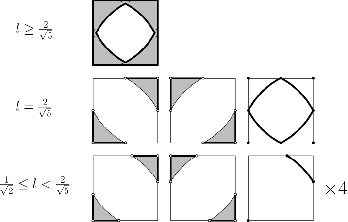
A quick illustration of this concept for squares makes it clear that these components can be quite interesting. If the square has side lengths , then it seems that has one non-trivial connected component consisting of the points
where is the set of vertices of , and is the open ball of radius around ; all points on the interior of the shape bounded by these circle arcs have no neighbours (Figure 3). If , then appears to have 3 non-trivial connected components:
where is the circle of radius around (Figure 3). For , the last of these components falls apart into 4 separate components consisting of a vertex and the arc .
There is a striking (partial) correspondence between the critical side lengths , and of the square for which the number of non-trivial connected components of changes, and the lengths at which the chromatic number changes [Kru08]—only the critical value for the chromatic number does not show up here. It would be interesting to study the case in more detail, and to investigate whether such a correspondence also holds for hypercubes.
6.2 Random walks
Our problem is obviously also related to random walk problems. In most of these problems, the step length has some continuous distribution (often exponential). Here, the step length is in all cases, and only the new direction is chosen (e.g., uniformly) at random. This leads to the question of determining the distribution for the location after a fixed number of steps. Probabilistic problems of this nature have been investigated thoroughly ever since Pearson asked the following question [Pea05].
A man starts from a point and walks yards in a straight line; he then turns through any angle whatever and walks another yards in a second straight line. He repeats this process times. I require the probability that after these stretches he is at a distance between and from his starting point, .
However, in related research, the space of the so called short uniform random walk is most often unbounded, i.e., (e.g., [BNSW11, BS16, Zho19]). There is at least some interest in bounded cases—as we have studied in a non probabilistic setting—as well, but then, too the step size may vary, and the boundary may be assumed to be reflexive (e.g., [CR87]).
Although we do not venture into the probabilistic realm in this paper, there are some obvious questions that this paper brings up. For example, we could ask essentially the same question as Pearson for bounded regions, but for a man who is aware of his surroundings and walks stretches of length without crossing the boundary of the region. Note that the starting point is of great influence in this problem, and a uniform distribution on the neighbourhood may either be a continuous one (if there is an infinite number of neighbours), or discrete (if the neighbourhood is finite, such as for the midpoint of ).
Some examples of such distributions after a small number of steps in squares of varying size are shown in Figure 4. These are estimated using independent Monte-Carlo simulations of the process.

As for Pearson’s question, we can also inquire about the distribution after an infinite number of steps. i.e., the stationary distribution of the random walk. This distribution may depend on the starting point when the is disconnected, or is only connected via a node of finite degree.
References
- [ACL+14] Maria Axenovich, J Choi, M Lastrina, T McKay, J Smith, and B Stanton. On the chromatic number of subsets of the euclidean plane. Graphs and Combinatorics, 30(1):71–81, 2014.
- [Bau98] Bruce L Bauslaugh. Tearing a strip off the plane. Journal of Graph Theory, 29(1):17–33, 1998.
- [BNSW11] Jonathan M Borwein, Dirk Nuyens, Armin Straub, and James Wan. Some arithmetic properties of short random walk integrals. The Ramanujan Journal, 26(1):109, 2011.
- [BS16] Jonathan M Borwein and Corwin W Sinnamon. A closed form for the density functions of random walks in odd dimensions. Bulletin of the Australian Mathematical Society, 93(2):330–339, 2016.
- [CR87] Brian Conolly and David Roberts. Random walk models for search with particular reference to a bounded region. European journal of operational research, 28(3):308–320, 1987.
- [FGK03] Kaspar Fischer, Bernd Gärtner, and Martin Kutz. Fast smallest-enclosing-ball computation in high dimensions. In European Symposium on Algorithms, pages 630–641. Springer, 2003.
- [KBVC18] A Kanel-Belov, V Voronov, and D Cherkashin. On the chromatic number of an infinitesimal plane layer. St. Petersburg Mathematical Journal, 29(5):761–775, 2018.
- [Kru08] Clyde P Kruskal. The chromatic number of the plane: the bounded case. Journal of Computer and System Sciences, 74(4):598–627, 2008.
- [Pea05] Karl Pearson. The problem of the random walk. Nature, 72(1865):294–294, 1905.
- [VHG+13] Evan VanderZee, Anil N Hirani, Damrong Guoy, Vadim Zharnitsky, and Edgar A Ramos. Geometric and combinatorial properties of well-centered triangulations in three and higher dimensions. Computational Geometry, 46(6):700–724, 2013.
- [VHGR10] Evan Vanderzee, Anil N Hirani, Damrong Guoy, and Edgar A Ramos. Well-centered triangulation. SIAM Journal on Scientific Computing, 31(6):4497–4523, 2010.
- [Zho19] Yajun Zhou. On borwein’s conjectures for planar uniform random walks. Journal of the Australian Mathematical Society, 107(3):392–411, 2019.