Control of Scanning Quantum Dot Microscopy
Abstract
Scanning quantum dot microscopy is a recently developed high-resolution microscopy technique that is based on atomic force microscopy and is capable of imaging the electrostatic potential of nanostructures like molecules or single atoms. Recently, it could be shown that it not only yields qualitatively but also quantitatively cutting edge images even on an atomic level. In this paper we present how control is a key enabling element to this. The developed control approach consists of a two-degree-of-freedom control framework that comprises a feedforward and a feedback part. For the latter we design two tailored feedback controllers. The feedforward part generates a reference for the current scanned line based on the previously scanned one. We discuss in detail various aspects of the presented control approach and its implications for scanning quantum dot microscopy. We evaluate the influence of the feedforward part and compare the two proposed feedback controllers. The proposed control algorithms speed up scanning quantum dot microscopy by more than a magnitude and enable to scan large sample areas.
I Introduction
An important aspect in nanotechnology is the determination of characteristics of the fundamental building blocks of matter, namely atoms and molecules. One of these characteristics are the electrostatic properties that govern in many cases the functionality of nanoscale objects and systems. This is particularly important for new materials and devices associated with nanoscale electronics, such as semiconductors. The investigation of electrostatics at the nanoscale becomes therefore more and more important and is a vivid field of ongoing research [1, 2, 3, 4, 5].

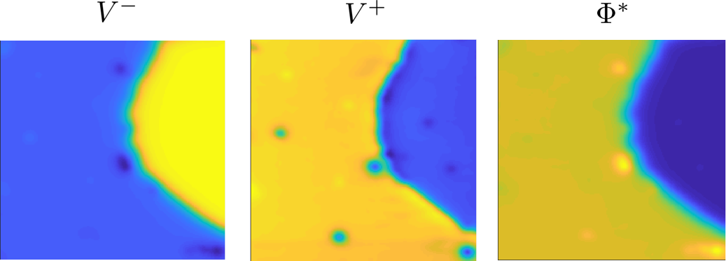
Scanning quantum dot microscopy (SQDM), introduced in [6, 7] allows to measure the electrostatic potentials of nanostructures with sub-nanometer resolution at large imaging distances. It generates 2D images of the electrostatic potential (Fig. 1). It furthermore allows to separately image the electrostatic potential and the surface topography. Recently it was shown in [5] that SQDM does not only generate qualitative but also quantitative images of the electrostatic potential of nanostructures. The paper also demonstrated large-scale imaging (Fig. 1), resolving both small (single atoms and molecules) and large structures (an island composed of several hundreds of molecules) in the same image, whereas in the previous publications of SQDM [6, 7] only isolated atoms and molecules were imaged independently of each other. Thereby, SQDM became a mature widely applicable microscopy technique for the area of nanotechnology.
This paper is the control engineering counterpart of [5], wherein the controller was only briefly mentioned. We present in detail the tailored two-degree-of-freedom control algorithm that is a key enabling element that turned SQDM into a well applicable microscopy technique. The controller is a variant of the one presented in [8], which included a Gaussian process as a feedforward signal generator. However, that approach is not yet ready for the deployment in the experiment because further research, in particular regarding the computational issues for the online learning of the Gaussian process, has to be conducted. Henceforth, the objective of this work is to present the controller version that was actually used in [5]. Opposed to the initial method of generating SQDM images based on spectroscopy grids (see [6]), the controller now allows to continuously scan the sample, which yields order-of-magnitude faster image generation and eliminates the need for spectroscopy. This puts it in line with other microscopy techniques like scanning tunneling microscopy [9] and atomic force microscopy [10]. Furthermore, the controller now also allows to scan images with highly varying electrostatic potentials. Previously, using spectroscopy grids one had to set up the spectrum range, which increases with the electrostatic potential, before starting the grid. This was a huge setback in speed if the electrostatic potential and with that the spectrum range was large because the entire voltage range had to be scanned.
After this introduction, the paper is structured as follows. Sec. II provides the fundamentals of scanning quantum dot microscopy. The 2DOF control framework is presented in Sec. III and thoroughly analyzed in simulations in Sec. IV. Further experimental results are presented in Sec. V and the paper is concluded in Sec. VI.
II Scanning Quantum Dot Microscopy
This section explains the working principle of scanning quantum dot microscopy and the associated image generation process. The process is analyzed and a model derived that will be used in Sec. IV-B for simulations.
II-A Working Principle

SQDM is able to measure electric surface potentials and allows to distinguish between topographical and electrostatic effects. It utilizes a frequency modulated non-contact atomic force microscope (NC-AFM) [10], operated in ultra-high vacuum and at a temperature of 5 K. The atomically sharp tip (Fig. 2) is mounted to a tuning fork (qPlus sensor [11]) that oscillates with a frequency of around 30 kHz, where is the free resonance frequency and is the frequency change that is caused by a vertical force gradient acting on the tip. Typically, this force is the result of the tip-sample interaction.
The AFM tip is decorated ([12, 13, 14, 15, 16]) with a quantum dot (QD)11 1 Currently a PTCDA (Perylenetetracarboxylic dianhydride) molecule serves as the QD., a nano-sized object whose energy levels can take only discrete values. Changes of the electrostatic potential of the surface can change the QD’s charge state via gating as an electron tunnels from the tip into the QD. This leads to an abrupt change in the tip-sample force. These tip-sample force changes are detected by the NC-AFM, effectively transducing the information about the electrostatic potential of, e.g. a nanostructure, into the measurable quantity . Monitoring the charging events of the QD while scanning the sample is the basic working principle of SQDM.
To detect the charging events, a bias voltage source is connected to the sample while the tip is grounded. The associated electrostatic potential that is generated by is superimposed on the intrinsic electrostatic surface potential of the sample . Accordingly, a change in then leads to a change of the effective electric potential at the QD. If this reaches a threshold value, a change in the QD’s charge state is triggered.
Charging of the QD leads to a change in the tip-sample force, whose gradient is proportional to for small amplitudes of the AFM tip oscillation (see [17]). The changes of the tip-sample force generated by the charging events appear in the so-called spectrum as features that we denote as dips (Fig. 3). The spectrum is the superposition of a parabola ([18]) and two dips, one at negative values and one at positive values. The dips separate intervals with different charge states of the QD.

We denote the voltage values at which the dips reach their minimum with and , or short . These values characterize the dips’ positions within the spectrum. By means of
| (1) |
the effective surface potential at the position of the tip can be calculated, where and are reference points. The actual surface potential can be recovered from through deconvolution in post-processing [19]. In the rest of this paper we will deal with unless otherwise indicated. For more details see [19].
II-B Original Image Generation Process
The image generation process that had been previously used in [6, 7] is as follows. The sample (Fig. 1) is discretized in pixels (Fig. 2) and the tip with the QD is moved from pixel to pixel. At the first pixel, a complete spectrum (like Fig. 3) is measured and the positions of the dips are determined. It has to be assumed that the interval in which will change while scanning the sample is approximately known a priori. For the following pixels, the bias voltage is swept accordingly within these two intervals (e.g. a voltage range of 0.2 V instead of 6 V for the complete spectrum). This results in the measurement of local dip spectra. After obtaining the local dip spectra for all pixels, the values are determined for each pixel and used in (1) to generate .
The main limitation of this image generation process is the required large total measurement time. For instance, measuring the local dip spectra takes about 3 s for each dip and pixel for a certain interval size. Hence, the determination of the complete maps in Fig. 4 would require 66.7 h.22 2 The data shown in Fig. 4 was generated by the proposed control approach in this paper, which results in significantly smaller measurement times. This severely limits the applicability of SQDM. In particular,
- •
the microscope is blocked for several hours for the generation of one image,
- •
the longer the measurement time, the higher the probability of failures, and
- •
effects like drift increase and deteriorate image quality.
Furthermore, obtaining images from a grid of spectra limits SQDM in several ways:
- •
Generation of fast and rough images for a first impression is not possible.
- •
- •
The measurement times of the local spectra increase if the aforementioned voltage intervals, wherein the dips move, increase. This can occur, for instance, for other substrate-sample combinations with stronger electrostatic variations and thus, reduce the applicability even further.
II-C Simulation Model
The controllers, as outlined in Section III, are going to be evaluated in simulations in Section IV. This requires a SQDM simulation model, which we derive in the following.

Fig. 5 illustrates the SQDM system in a block diagram. In the experiment, the current bias voltage and tip position lead to an oscillation frequency of the tuning fork different from the free resonance frequency . Hence, and are the inputs to the system and the frequency change is the output. The bias voltage is the control input to the system and can be chosen freely, whereas the tip position changes according to the raster scanning pattern as shown in Fig. 2. As changes, the frequency changes almost instantaneously according to Fig. 3. Therefore, the first block in Fig. 5 can be considered stationary. The relatively small frequency change (only up to a few Hz, compared to 30 kHz of the free resonance frequency ) is determined from the oscillation signal using a phase-locked loop (PLL), which is modeled as a first order system with bandwidth and whose output is corrupted by white Gaussian noise.
To simulate SQDM and the image generation process, the spectrum has to be available as an analytic function. It consists of a parabola and the two dips, which we model as Gaussian curves33 3 Note that in the actual experiment, the shape of the dips is somewhere between a Gaussian curve and a half-circle, depending on the chosen tip oscillation amplitude, the value of , and the width of the electronic level of the QD. See also [20]. . The ansatz for the spectrum is
| (2) |
with the parabola function
and the Gaussian curves
| (3) | ||||
| (4) |
for the dips, where are the respective depth, position, and width of the dips. The function in (4) is the polynomial . The parameters in (2), (3), and (4) are then fitted using experimental data. The resulting fit in Fig. 3 and Tab. I shows that the proposed ansatz is well suited to model the experimentally acquired spectrum.
III Controller Development
The effective electrostatic potential of the sample at the position of the tip changes in the three dimensional space. However, since SQDM is based on AFM, only 2D images can be generated. Therefore, we consider in the following that, according to (1), depends in turn on the quantities , i.e., . The values are a priori unknown, cannot be measured directly, and change with the tip position . Therefore, SQDM with the changing values can be regarded as a parameter varying system and the objective of this paper is to design a control framework that automatically determines and tracks the unknown parameters while scanning the sample.
As outlined, cannot be measured directly and a model of the respective dynamics is unavailable because it depends, besides the scan speed, on the electrostatic potential, which itself is unknown. Thus, a potential control approach has to adapt indirectly, based on a quantity that can be measured, in this case the frequency change . Hence, we are looking for a control law .
In the following we present a two-degree-of-freedom (2DOF) control approach, consisting of a feedback and a feedforward (FF) part (Fig. 6). We furthermore develop two different feedback controllers, leading to two different versions of the 2DOF controller. The first feedback controller is an extremum seeking controller (ESC) and the second controller is called slope tracking controller (STC). The central idea to both controllers is, instead of measuring the dip spectrum (time consuming, contains a lot of unnecessary data), to track one specific reference point in each dip. A major difference between the ESC and the STC is this reference point. While the ESC tracks directly , the STC tracks a point on the dip’s slope (thus the name).
The individual 2DOF parts will be discussed in more detail in the remainder of this section.

III-A Extremum Seeking Control
The fact that characterize the minima of the local convex dips satisfying
| (5) | ||||
| (6) |
can be exploited for the determination of . Since is measured online by the phase-locked loop, the minima of can be determined continuously by appropriately adapting the input in (5) and (6) during the scanning process.
This can be achieved by employing methods of extremum seeking control [21, 22]. As the name indicates, these methods are designed to find the extremum, i.e., a minimum or a maximum, of the output of a given system. The core principle includes a seeking element that continuously samples the output signal at the current operating point to obtain some kind of direction or gradient information. If a measure of the gradient is detected, the current operating point is changed accordingly. If the optimum is reached, the gradient is zero and the operating point is not changed anymore. Thus, ESC approaches are closely related to optimization and are therefore also called real-time optimization methods [21]. In principle, an ESC can be realized with many different optimization methods, though they have to satisfy a variety of additional properties, such as, for instance, low computational load or the ability to deal with constraints.
Works on extremum seeking date back to as early as 1922 [23] or 1951 [24]. Though many other works were published in the second half of the 21th century (see [25]), it wasn’t until the paper of [26] in the year 2000 that provided the first general stability analysis of ESC. Since then, interest has sparked again and found its realizations in applications such as anti-lock-breaking systems [27, 28], maximum-power-point-tracking [29, 30], source seeking [28, 31], beam control in particle accelerators [32], or the control of plasma in a Tokamak reactor [33]. Theoretic extensions for discrete time systems [34], for multivariable systems [35], systems with partial model information [25, 36], and further results on stability [37, 32] have been presented. Generalizations of the ESC scheme such as a unifying framework [38] and with other optimization approaches, such as newton like extremum seeking [39, 40], stochastic [41, 42] and a non-gradient approach [43] have been developed too. For extensive lists of further publications see [44, 22, 32].
In this work we employ an adapted version of the approach of [26] as shown in Fig. 7. In this setup we deal with a local convex function for which there exists a minimum at . At this minimum we have naturally . To search for , a dither signal is used to perturb the current . The resulting signal is passed through a high pass filter to eliminate any constant offsets. The filtered signal is then multiplied by the phase shifted dither signal44 4 The phase of is shifted by the high pass filter by . In order to be in phase, the dither signal that is multiplied with is shifted also by . and low pass filtered with . This leads to and it can be shown that
at the current operating point . Choosing , one obtains
i.e., tends to the negative gradient of . Hence, can be used subsequently to implement a gradient descent approach, realized by the integration of , turning into an estimation of the minimizer .

Applied to SQDM we have as a local convex function and the ESC computes the derivative by modulating the dither signal onto the signal. Since characterizes the dips’ minima, it also characterizes exactly the value of . Thus, if a potential controller regulates to zero55 5 Note that only one dip can be tracked at a time., it automatically yields . Therefore, is used as the reference and the gradient descent is achieved by using an integral controller
that minimizes the error with and . The voltage applied to the AFM cantilever is
where is the feedforward signal computed as detailed in Section III-C. Note that the signal without the dither signal is used for image generation. The corresponding block diagram is depicted in Fig. 8.

The ESC parameters that need to be chosen are the dither signal amplitude and frequency , the low and high pass filter cut-off frequencies and , and the control gain . In the following we present some general guidelines for choosing these parameters based on the characteristics of the respective dip and the phase-locked loop.
III-A1 Dither Signal
The interval in which the applied bias voltage varies locally is . The gradient of the dip is then approximated within this interval, i.e., an average gradient around the current bias voltage is computed. A natural upper limit is therefore the dip width itself. On the other hand, the smaller , the more accurate the gradient at . However, the measurements for the gradient computation are corrupted by noise, which poses a lower limit on . Thus, we get
where should be chosen as small as possible.
Regarding the choice of the dither signal frequency : the higher the frequency, the faster the gradient estimate converges but also the higher the variance of the estimate. Additionally, if is much larger than the system’s bandwidth, the dither signal is damped and shifted significantly and in consequence the gradient computation deteriorates. Hence, an upper bound depends on the maximum bandwidth of the system dynamics. In SQDM, the phase-locked loop is the limiting element with its bandwidth . We have found
to work well, where larger values decrease convergence time but increase variance.
III-A2 Filter Cut-Off Frequencies
The objective of the high pass filter is to remove the constant offset of the signal. This can be sufficiently fast achieved for
The objective of the low pass filter is to smoothen the signal . The smaller the stronger the smoothing. The stronger the smoothing, the less oscillatory the gradient approximation becomes but also the slower the convergence. Hence, choosing is a trade-off between convergence speed and variance, similar to . We have found that
works well. Accordingly, can be chosen within this interval, depending on the objective of fast convergence (fast scanning) or small variance.
III-A3 Phase Shift
The phase-locked loop and the high pass filter introduce an additional phase shift
w.r.t. the dither signal, where is the PLL transfer function and the high pass filter transfer function. This can be accounted for by adding the same phase shift to the dither signal that is multiplied with the high pass outcoming signal (see Fig. 7).
III-A4 Control Gain
To facilitate gain tuning, we define via
| (7) |
where is the new tunable ESC gain. This redefinition automatically compensates the amplitude change of introduced by the PLL and the high pass filter. This way the PLL and the high pass filter can be changed without influencing the amplitude. Note that the low pass filter is not included in (7) because then one loses the possibility of adjusting the convergence of independently of that of .
The larger , the faster the convergence to the minimum but also the more oscillatory the estimated minimizer . Hence, the larger , the faster we can scan the sample but at the cost of less accurate tracking. In particular, oscillations due to high values eventually appear in the final image as noise. Furthermore, if the oscillations in become too large, the dip might be lost. For instance, when the negative dip is tracked the oscillations might cause to leave the dip towards the left side of the dip. There the gradient descent then leads the controller to further decrease the value down the parabola, making it impossible to recover the dip.
III-B Slope Tracking Control
Another possibility to control SQDM is by tracking a point on the dips’ slope (Fig. 9), instead of tracking the dips’ minima. The resulting value is then set as the reference value for the whole sample and the deviations are used directly as an error to the integral controller
| (8) |
that adapts accordingly with . The resulting voltage applied to the AFM cantilever is
with computed as detailed in Section III-C. The resulting block diagram is depicted in Fig. 10.


The STC parameters that need to be chosen are the exact position of the reference point and the control gain .
III-B1 Reference Point
The choice of the STC reference point is very important. In particular because most of the values of a dip appear three times in the local spectrum around the respective dip (see Fig. 9). We choose to lie on the inner slope of the dips (i.e., on the right slope of the negative dip and on the left slope of the positive dip) and detail the reasons in the following.
First note, that the inner slope is always larger than the outer slope (compare Fig. 3 and Fig. 9), which suggests better control performance on the inner slope. Second, if the reference point is located on the inner slope, according to (8) the controller is able to drive to even if has left the dips towards the vertex of the parabola (the sign of doesn’t change). This would not be the case if the reference point was chosen to lie on the outer slope and had left the dips towards the part of the parabola where values decrease indefinitely. In that case the controller would drive the bias voltage to even larger absolute values until the corresponding value on the parabola is reached (crossing of the dashed black line and the blue parabola on the left side in Fig. 9). In general, the STC won’t be able to recover the dip in that case.
Regarding the exact position, should lie relatively far away from the dip minimum at because this is another critical point for the STC. If moves over this point (e.g. for the negative dip) the control error becomes smaller instead of larger, which automatically has a deteriorating effect on the control performance and increases the probability that the dip is left towards the part of the parabola where values decrease indefinitely.
III-B2 Controller Gain
Regarding the STC gain , the same holds as for the ESC gain . The larger the faster the convergence to but also the more oscillatory. Thus, the larger the faster the sample can be scanned but at the cost of less accurate tracking.
The STC does not require the computation of the derivative and is therefore faster. However, it introduces a systematic error due to the difference between and the value at the STC reference (approximately66 6 Since the positive dip is wider, this error is larger for the positive dip. in Fig. 9) that we denote by . Additionally, this error is not constant and changes while scanning because when the dip changes its position it slides the parabola up- or downwards. For further clarification imagine that the negative dip moves vertically upwards (no horizontal movement). In that case, does not change but changes to more negative values, moving closer to . Hence, decreases as the dip moves vertically upwards and decreases as the dip moves downwards. This effect also occurs when the dip moves along the parabola because there is always a vertical motion component. In particular, the effect is larger for the positive dip because it is typically located at steeper parts of the parabola where the vertical motion is more pronounced.
A comparison of the advantages and drawbacks of the ESC and STC is provided in Tab. II.
| Advantages | Drawbacks | |
|---|---|---|
| ESC | robust | slow, many parameters |
| STC | fast, few parameters | delicate, systematic error |
III-C Feedforward
2DOF control approaches are well known in scanning probe techniques like scanning tunneling or atomic force microscopy. The control objective is usually to steer the piezo stages that govern the movement of the microscope tip in , , and direction. The -piezo is controlled according to the topography feedback signal (e.g. tunneling current in scanning tunneling microscopy or force in contact mode atomic force microscopy [45, 46]), whereas the piezos in and direction are controlled such that the tip follows specific reference trajectories in the -plane that implement the raster scanning pattern. For the main scanning direction, this is usually a triangular signal [47]. The controllers are often based on models of the respective piezo stages. The feedforward part of the 2DOF controllers is therefore also usually model based and techniques like , -optimal, model inversion, or iterative learning control are employed. For good overviews on this topic see [47, 48, 49, 50, 51, 52].
As already detailed throughout this section, the objective is to track the dips’ minima (with the ESC) or a point on the dips’ inner slope (with the STC). This objective is taken care of by the respective feedback controller. However, as already mentioned in Section III-B, it is possible (and has occurred) that the dips change their position faster than the respective controller can adapt the bias voltage, which eventually leads to the controller “losing the dip”. A combination of a rapid change of the electrostatic potential, a high scan speed, and the controller dynamics is usually the cause. In that case, the scanning process has to be aborted and restarted from the beginning.
This risk can be substantially reduced by the generation of an appropriate feedforward signal, such that the initial value for each controller at each tip position stays always within the dips’ interval. In that way, the feedforward has not only the potential for increased performance, and with that eventually higher scan speeds, but is even essential for correct operation of SQDM.
Since an a priori model of the electrostatic potential is not available, a natural choice is an approach that is based on the previously scanned line. Fig. 11 shows a block diagram of the feedforward signal generator for SQDM, which comprises the following elements and features.

- •
Buffer: The values of the currently scanned line are stored in a buffer alongside the indexing values within the line. Hence, is the fast scan direction. At the same time, already stored values of the previously scanned line are used as a basis for the feedforward signal of the current line.
- •
Filter: The measured and buffered values are corrupted by noise and small ripples caused by the ESC (if this is used for control), which have a deteriorating effect on the control performance, especially in regions where the electrostatic potential is relatively flat. Therefore, while scanning the current line , the previously measured values are smoothed to generate the feedforward signal using the mean filter
with filter window length .
- •
Scan speed adaptation: The previous line is indexed using the measured -position values. In the current line scan, the active -position is determined and used for picking the right reference value. This allows for varying scan speed within a line.
This approach to generate the feedforward signal is simple, straightforward to implement, yet practically powerful. By adding to , the controller has only to correct the difference between the current and the previous line. This results in a decreased control error and therewith a decreased probability that the “dips are lost”. Accordingly, the scan speed can be increased while maintaining the same image quality.
IV Simulations
In this section, we simulate the SQDM process together with the ESC and the STC and evaluate their performances qualitatively and quantitatively. To this end, we use the simulation model of Section II-C implemented in MATLAB/Simulink. We use a fixed-step ode3 (Bogacki-Shampine) solver with a sampling time of . Experimentally acquired spectra (Fig. 12) and the maps of Fig. 4 are used as reference data. The cutoff frequency of the phase-locked loop was determined by fitting a step response and was computed as . The normally distributed white noise has a standard deviation of . The parameters of the two controllers are listed in Tab. III.

| Negative Dip | Positive Dip |
| ESC | ESC |
| STC | STC |
IV-A Influence of the Dip Parameters
In Sec. III we have established a connection, in the form of constraints, between some of the controllers’ parameters and the parameters of the dips and the phase-locked loop. Here we furthermore investigate how the controllers’ performance is influenced by the dips’ depth and width .
As can be seen in Fig. 13 and Fig. 14, the deeper and narrower, i.e., the sharper the negative dip, the better because the faster the convergence. The same holds for the positive dip, as well as using the STC because sharper dips have steeper slopes, which improve tracking. We omit the corresponding plots for the sake of brevity. Hence practitioners of SQDM should aim for sharp dips. This can be achieved, for instance, with small oscillation amplitudes of the microscope cantilever [20]. However, at the same time such amplitudes increase the noise, which ultimately imposes a lower bound on the oscillation amplitude. Thus, the selection of the oscillation amplitude is a trade-off.


IV-B Simulation Results
We now compare the ESC and STC with and without feedforward using the experimentally acquired reference data. We start with an exemplary time evolution of the involved signals and illustrate the influence of the feedforward. Afterwards we turn our attention to the whole image generation and discuss the final images qualitatively and quantitatively. Using the same measures, we also quantify the influence of the scan speed on the image quality.
IV-B1 Time Evolution
In Fig. 15 and Fig. 16 exemplary time evolutions of the signal for the ESC and STC without and with feedforward are shown. Both simulations were performed with a scanning time of for the respective dip map. To mimic the experiment, each line is scanned back and forth. This results in approximately for each single line scan, which in turn equals a scanning speed of approximately 33.3 Å/s with the given area of 600600 Å.
In case of the negative dip (Fig. 15), at the beginning of the depicted evolution all four controller instances are able to adequately track the dip, though the STC with a constant error due to the fact that it tracks a point on the dips’ slope. As the variations in the electric potential increase, both controllers without the feedforward are unable to fully follow the reference. The ESC is unable to follow the variations (beginning around ) and the STC loses the reference around . In case of the positive dip (Fig. 16), the STC without feedforward again loses the dip (around ) and the ESC tracking results in larger errors for the shown plot as compared to its version with feedforward. Indeed at later times, which are not depicted for reasons of clarity, the ESC without feedforward presents the same behavior as in Fig. 15, where it is unable to follow the variations. Hence, we can conclude at this point that with feedforward the probability of both controllers successfully tracking the dips is significantly higher and the resulting tracking error is reduced.


IV-B2 Image Plots
Now we turn to the simulation of the complete scans of the negative and positive dip maps and the resulting electrostatic potential computed by (1). For the sake of brevity we provide only the final images.
The two resulting potential images of the ESC+FF (Fig. 17) and STC+FF (Fig. 18) look almost identical to the reference in Fig. 1 and 4. Hence, the dips are successfully tracked over the whole sample. The respective error images (Fig. 19 and Fig. 20) reveal that the errors are in the range of to . As the total variation is , the relative errors w.r.t. this variation are to . Furthermore, it can be seen that the STC version of the 2DOF controller performs slightly better with smaller errors on average and with less noise. On the other hand, above the molecular island (right part in Fig. 20) it can be observed that the average STC error is shifted roughly about 1.5 mV towards more negative values. This is due to the change of the systematic STC error as discussed in Section III-B2. Nevertheless, the STC performs slightly better than the ESC, as is also confirmed in Tab. IV, where we quantify the image quality using the image mean-square error (MSE) and the image peak signal-to-noise ratio (PSNR) per pixel respectively77 7 These measures are often used in imaging science as objective quality measures. See, for instance, [53, 54]..
The total scan time for each of the results in Fig. 17 and Fig. 18 was 4 h. This is approximately 17 times faster than the original image generation process based on spectroscopy grids that would have taken 66.7 h (see Sec. II-B).


IV-B3 Influence of scan time
Finally we investigate how the resulting image quality is influenced by the scan time . To this end we repeat the simulation with scan times from 2 h to 6 h. This equals scan speeds of 33.3 Å/s to 11.1 Å/s. After every simulation we compute the MSE and PSNR of the resulting electrostatic potential image and plot it over . The results are depicted Fig. 21. The slower we scan, the slower the variations and thus, the feedback controllers are better able to follow the references, which is reflected in lower MSE and larger PSNR values.

Remark: Of course, if the variability in the electrostatic potential is large enough, there exists always a scan time that is too small such that good tracking is not possible, even with the feedforward. Nevertheless, we could show in this section that the probability to successfully track the reference is significantly higher if the proposed feedforward signal is employed and that reasonable scan times can be reached for large samples.
V Experimental Results
In this section, we present information on the implementation of the 2DOF controller in the experimental setup, discuss the SQDM operation procedure, and present further experimentally generated images of nanoscale samples with the presented control approach of this work.
V-A Implementation
The 2DOF controller is built in MATLAB/Simulink and automatically converted into C-code and then loaded to and executed on a ds1104 controller board by dSPACE. The controller board is mounted into a standard desktop PC and connected via analog-digital and digital-analog converters to a Createc non-contact atomic force/scanning tunneling microscope (STM/NC-AFM) that operates at and under ultra high vacuum. The microscope is equipped with a qPlus sensor ([55]) tuning fork with resonance frequency , stiffness . An amplitude of was used in the measurements.
V-B Image Generation Procedure
The procedure used to acquire a new image is as follows:
- 1.
Move to first pixel and measure the local spectrum of the respective dip .
- 2.
Adjust manually to the reference point (the selection of the reference point depends on whether the STC or the ESC is used, see Fig. 9).
- 3.
Start the 2DOF controller.
- 4.
Start the raster scanning protocol.
- 5.
Enable the feedforward after one or more lines have been scanned.
- 6.
Increase scanning speed desired.
- 7.
Finish the scan for the current dip .
- 8.
Goto 1) and repeat for the other dip .
V-C Images
Here we show a so far unpublished result obtained with the described control approach. The 2DOF controller with the STC has been employed together with the above described procedure to investigate the electrostatic potential of the sample presented in Fig. 22. The resulting SQDM image is shown in Fig. 23. The sample shows three features on a Ag(111) surface, namely a PTCDA molecule (top left), a PTCDA-Ag2 complex (top right), and a single Ag adatom (bottom).


VI Conclusion
In this paper we have presented a two-degree-of-freedom control approach for scanning quantum dot microscopy. The approach consists of a feedback part and a feedforward signal generator, where the latter is based on the previous line scan. For the feedback part we have presented two different controllers, namely an extremum seeking control approach that directly tracks the dip minimum and a controller that tracks a reference point on the dip slope. We have discussed the individual working principles, respective advantages and drawbacks, and provided guidelines for controller parameterization tailored to scanning quantum dot microscopy.
In simulations we could show how the utilization of the feedforward decreases the probability of losing the dips and decreases the resulting image error at the same time. This leads to a several times faster image generation process and enables to scan larger images in reasonable time than before, which was also verified in experiments. In addition, the presented control approach now allows to continuously scan a sample, which puts scanning quantum dot microscopy in line with other scanning probe microscopy techniques like scanning tunneling or atomic force microscopy.
Furthermore, we could also show that the sharpness of the dips plays a central role in the control performance, which led to the recommendation that one should aim for sharper dips if possible.
The next steps are going to include an automatic gain adaptation for varying scan speeds and the improvement of the feedforward by using previous lines to generate an accurate prediction of the current line using a Gaussian process and implement it in the experimental setup [8].
References
- [1] P. Matyba, K. Maturova, M. Kemerink, N. D. Robinson, and L. Edman, “The dynamic organic p-n junction,” Nature Materials, vol. 8, no. 8, pp. 672–676, 2009.
- [2] C. Musumeci, A. Liscio, V. Palermo, and P. Samorì, “Electronic characterization of supramolecular materials at the nanoscale by conductive atomic force and Kelvin probe force microscopies,” Materials Today, vol. 17, no. 10, pp. 504–517, 2014.
- [3] F. Fuchs, F. Caffy, R. Demadrille, T. Meilin, and B. Greivin, “High-resolution Kelvin probe force microscopy imaging of interface dipoles and photogenerated charges in organic donor–acceptor photovoltaic blends,” ACS nano, vol. 10, no. 1, pp. 739–746, 2016.
- [4] Y. Hu, V. Pecunia, L. Jiang, C.-A. Di, X. Gao, and H. Sirringhaus, “Scanning Kelvin probe microscopy investigation of the role of minority carriers on the switching characteristics of organic field-effect transistors,” Advanced Materials, vol. 28, no. 23, pp. 4713–4719, 2016.
- [5] C. Wagner, M. F. Green, M. Maiworm, P. Leinen, T. Esat, N. Ferri, N. Friedrich, R. Findeisen, A. Tkatchenko, R. Temirov, and F. S. Tautz, “Quantitative imaging of electric surface potentials with single-atom sensitivity,” Nature Materials, 2019.
- [6] C. Wagner, M. F. Green, P. Leinen, T. Deilmann, P. Krüger, M. Rohlfing, R. Temirov, and F. S. Tautz, “Scanning quantum dot microscopy,” Physical Review Letters, vol. 115, p. 026101, 2015.
- [7] M. F. Green, C. Wagner, P. Leinen, T. Deilmann, P. Krüger, M. Rohlfing, F. S. Tautz, and R. Temirov, “Scanning quantum dot microscopy: A quantitative method to measure local electrostatic potential near surfaces,” Japanese Journal of Applied Physics, vol. 55, no. 8S1, p. 08NA04, 2016.
- [8] M. Maiworm, C. Wagner, R. Temirov, F. S. Tautz, and R. Findeisen, “Two-degree-of-freedom control combining machine learning and extremum seeking for fast scanning quantum dot microscopy,” in American Control Conference (ACC), (Milwaukee, USA), pp. 4360–4366, IEEE, 2018.
- [9] G. Binnig, H. Rohrer, C. Gerber, and E. Weibel, “Surface studies by scanning tunneling microscopy,” Physical review letters, vol. 49, no. 1, p. 57, 1982.
- [10] T. Albrecht, P. Grütter, D. Horne, and D. Rugar, “Frequency modulation detection using high-Q cantilevers for enhanced force microscope sensitivity,” Journal of Applied Physics, vol. 69, no. 2, pp. 668–673, 1991.
- [11] F. J. Giessibl, “Advances in atomic force microscopy,” Reviews of modern physics, vol. 75, no. 3, p. 949, 2003.
- [12] C. Toher, R. Temirov, A. Greuling, F. Pump, M. Kaczmarski, G. Cuniberti, M. Rohlfing, and F. Tautz, “Electrical transport through a mechanically gated molecular wire,” Physical Review B, vol. 83, no. 15, p. 155402, 2011.
- [13] N. Fournier, C. Wagner, C. Weiss, R. Temirov, and F. Tautz, “Force-controlled lifting of molecular wires,” Physical Review B, vol. 84, no. 3, p. 035435, 2011.
- [14] C. Wagner, N. Fournier, F. Tautz, and R. Temirov, “Measurement of the binding energies of the organic-metal perylene-teracarboxylic-dianhydride/Au (111) bonds by molecular manipulation using an atomic force microscope,” Physical Review Letters, vol. 109, no. 7, p. 076102, 2012.
- [15] C. Wagner, N. Fournier, V. G. Ruiz, C. Li, K. Müllen, M. Rohlfing, A. Tkatchenko, R. Temirov, and F. S. Tautz, “Non-additivity of molecule-surface van der Waals potentials from force measurements,” Nature Communications, vol. 5, 2014.
- [16] R. Findeisen, M. A. Grover, C. Wagner, M. Maiworm, R. Temirov, F. S. Tautz, M. V. Salapaka, S. Salapaka, R. D. Braatz, and S. O. R. Moheimani, “Control on a molecular scale: A perspective,” in American Control Conference, (Boston, USA), pp. 3069–3082, IEEE, 2016.
- [17] F. J. Giessibl, “Forces and frequency shifts in atomic-resolution dynamic-force microscopy,” Physical Review B, vol. 56, no. 24, p. 16010, 1997.
- [18] L. Gross, F. Mohn, P. Liljeroth, J. Repp, F. J. Giessibl, and G. Meyer, “Measuring the charge state of an adatom with noncontact atomic force microscopy,” Science, vol. 324, no. 5933, pp. 1428–1431, 2009.
- [19] C. Wagner and F. S. Tautz, “The theory of scanning quantum dot microscopy,” Journal of Physics: Condensed Matter, vol. 31, no. 47, p. 475901, 2019.
- [20] N. Kocić, P. Weiderer, S. Keller, S. Decurtins, S.-X. Liu, and J. Repp, “Periodic charging of individual molecules coupled to the motion of an atomic force microscopy tip,” Nano Letters, vol. 15, no. 7, pp. 4406–4411, 2015.
- [21] K. B. Ariyur and M. Krstić, Real-Time Optimization by Extremum-Seeking Control. John Wiley and Sons Inc., 2003.
- [22] C. Zhang and R. Ordóñez, Extremum-seeking control and applications: A numerical optimization-based approach. Advances in Industrial Control, Springer-Verlag London, 2012.
- [23] M. Leblanc, “Sur l’electrification des chemins de fer au moyen de courants alternatifs de frequence elevee,” Revue Générale de l’Électricité, vol. 12, no. 8, pp. 275–277, 1922.
- [24] C. S. Draper and Y. T. Li, Principles of optimalizing control systems and an application to the internal combustion engine. American Society of Mechanical Engineers, 1951.
- [25] M. Guay and T. Zhang, “Adaptive extremum seeking control of nonlinear dynamic systems with parametric uncertainties,” Automatica, vol. 39, no. 7, pp. 1283–1293, 2003.
- [26] M. Krstić and H.-H. Wang, “Stability of extremum seeking feedback for general nonlinear dynamic systems,” Automatica, vol. 36, no. 4, pp. 595–601, 2000.
- [27] H. Yu and U. Ozguner, “Extremum-seeking control strategy for ABS system with time delay,” in American Control Conference, vol. 5, pp. 3753–3758, 2002.
- [28] C. Zhang and R. Ordóñez, “Numerical optimization-based extremum seeking control with application to ABS design,” IEEE Transactions on Automatic Control, vol. 52, no. 3, pp. 454–467, 2007.
- [29] R. Leyva, C. Alonso, I. Queinnec, A. Cid-Pastor, D. Lagrange, and L. Martinez-Salamero, “MPPT of photovoltaic systems using extremum–seeking control,” IEEE Transactions on Aerospace and Electronic Systems, vol. 42, no. 1, pp. 249–258, 2006.
- [30] S. Brunton, C. Rowley, S. Kulkarni, and C. Clarkson, “Maximum power point tracking for photovoltaic optimization using ripple-based extremum seeking control,” IEEE Transactions on Power Electronics, vol. 25, no. 10, pp. 2531–2540, 2010.
- [31] J. Cochran and M. Krstić, “Nonholonomic source seeking with tuning of angular velocity,” IEEE Transactions on Automatic Control, vol. 54, no. 4, pp. 717–731, 2009.
- [32] A. Scheinker and M. Krstić, Model-free stabilization by extremum seeking. Springer, 2017.
- [33] C. Centioli, F. Iannone, G. Mazza, M. Panella, L. Pangione, S. Podda, A. Tuccillo, V. Vitale, and L. Zaccarian, “Maximization of the lower hybrid power coupling in the frascati tokamak upgrade via extremum seeking,” Control Engineering Practice, vol. 16, no. 12, pp. 1468–1478, 2008.
- [34] J.-Y. Choi, M. Krstić, K. B. Ariyur, and J. S. Lee, “Extremum seeking control for discrete-time systems,” IEEE Transactions on Automatic Control, vol. 47, no. 2, pp. 318–323, 2002.
- [35] M. A. Rotea, “Analysis of multivariable extremum seeking algorithms,” in American Control Conference (ACC), no. 6, pp. 433–437, IEEE, 2000.
- [36] V. Adetola and M. Guay, “Adaptive output feedback extremum seeking receding horizon control of linear systems,” Journal of Process Control, vol. 16, no. 5, pp. 521–533, 2006.
- [37] Y. Tan, D. Nešić, and I. Mareels, “On non-local stability properties of extremum seeking control,” Automatica, vol. 42, no. 6, pp. 889–903, 2006.
- [38] D. Nešić, A. Mohammadi, and C. Manzie, “A framework for extremum seeking control of systems with parameter uncertainties,” IEEE Transactions on Automatic Control, vol. 58, no. 2, pp. 435–448, 2012.
- [39] W. H. Moase, C. Manzie, and M. J. Brear, “Newton-like extremum-seeking part I: Theory,” in Conference on Decision and Control (CDC) held jointly with Chinese Control Conference, pp. 3839–3844, IEEE, 2009.
- [40] A. Ghaffari, M. Krstić, and D. Nešić, “Multivariable newton-based extremum seeking,” Automatica, vol. 48, no. 8, pp. 1759–1767, 2012.
- [41] S.-J. Liu and M. Krstić, Stochastic Averaging and Stochastic Extremum Seeking. Springer-Verlag London, 2012.
- [42] S.-J. Liu and M. Krstić, “Newton-based stochastic extremum seeking,” Automatica, vol. 50, no. 3, pp. 952–961, 2014.
- [43] D. Nešić, T. Nguyen, Y. Tan, and C. Manzie, “A non-gradient approach to global extremum seeking: An adaptation of the Shubert algorithm,” Automatica, vol. 49, no. 3, pp. 809–815, 2013.
- [44] Y. Tan, W. H. Moase, C. Manzie, D. Nešić, and I. Mareels, “Extremum seeking from 1922 to 2010,” in Chinese Control Conference, pp. 14–26, IEEE, 2010.
- [45] G. Schitter, A. Stemmer, and F. Allgower, “Robust 2DOF-control of a piezoelectric tube scanner for high speed atomic force microscopy,” in American Control Conference, pp. 3720–3725, 2003.
- [46] G. Schitter, F. Allgöwer, and A. Stemmer, “A new control strategy for high-speed atomic force microscopy,” Nanotechnology, vol. 15, no. 1, p. 108, 2004.
- [47] L. Y. Pao, J. Butterworth, and D. Y. Abramovitch, “Combined feedforward/feedback control of atomic force microscopes,” in American Control Conference, pp. 3509–3515, IEEE, 2007.
- [48] S. Devasia, E. Eleftheriou, and S. R. Moheimani, “A survey of control issues in nanopositioning,” IEEE Transactions on Control Systems Technology, vol. 15, no. 5, pp. 802–823, 2007.
- [49] G. M. Clayton, S. Tien, K. K. Leang, Q. Zou, and S. Devasia, “A review of feedforward control approaches in nanopositioning for high-speed SPM,” Journal of Dynamic Systems, Measurement, and Control, vol. 131, no. 6, p. 061101, 2009.
- [50] K. K. Leang, Q. Zou, and S. Devasia, “Feedforward control of piezoactuators in atomic force microscope systems,” IEEE Control Systems Magazine, vol. 29, no. 1, pp. 70–82, 2009.
- [51] Y. Yong, S. R. Moheimani, B. J. Kenton, and K. Leang, “Invited review article: High-speed flexure-guided nanopositioning: Mechanical design and control issues,” Review of scientific instruments, vol. 83, no. 12, p. 121101, 2012.
- [52] G. Gu, L. Zhu, C. Su, H. Ding, and S. Fatikow, “Modeling and control of piezo-actuated nanopositioning stages: A survey,” IEEE Transactions on Automation Science and Engineering, vol. 13, no. 1, pp. 313–332, 2016.
- [53] I. Avcibaş, B. Sankur, and K. Sayood, “Statistical evaluation of image quality measures,” Journal of Electronic Imaging, vol. 11, no. 2, pp. 206–223, 2002.
- [54] H. R. Sheikh and A. C. Bovik, “Image information and visual quality,” IEEE Transactions on Image Processing, vol. 15, no. 2, pp. 430–444, 2006.
- [55] F. J. Gießibl, S. Hembacher, M. Herz, C. Schiller, and J. Mannhart, “Stability considerations and implementation of cantilevers allowing dynamic force microscopy with optimal resolution: the qPlus sensor,” Nanotechnology, vol. 15, no. 2, p. S79, 2004.