Learning logic programs by explaining their failuresJournal: Machine learning
Abstract
Scientists form hypotheses and experimentally test them. If a hypothesis fails (is refuted), scientists try to explain the failure to eliminate other hypotheses. The more precise the failure analysis the more hypotheses can be eliminated. Thus inspired, we introduce failure explanation techniques for inductive logic programming. Given a hypothesis represented as a logic program, we test it on examples. If a hypothesis fails, we explain the failure in terms of failing sub-programs. In case a positive example fails, we identify failing sub-programs at the granularity of literals. We introduce a failure explanation algorithm based on analysing branches of SLD-trees. We integrate a meta-interpreter based implementation of this algorithm with the test-stage of the Popper ILP system. We show that fine-grained failure analysis allows for learning fine-grained constraints on the hypothesis space. Our experimental results show that explaining failures can drastically reduce hypothesis space exploration and learning times.
Keywords:
Relational Learning; Inductive Logic Programming; failure explanation1 Introduction
Explanations are ubiquitous in our cognitive lives keil2000explanation. They are crucial to the process of forming hypotheses, testing them on data, analysing the results, and forming new hypotheses, that is to say, to science popper2002conjectures. For instance, imagine Alice is a chemist trying to synthesise a vial of a compound from two substances (e.g. synth(thaum,slood,octiron)). Alice can perform actions, such as fill a vial with a substance (fill(Vial,Sub)) or mix two vials (mix(V1,V2,V3)), and sequence them to form a hypothesis, e.g.:
synth(A,B,C) fill(V1,A), fill(V1,B), mix(V1,V1,C)
This hypothesis says that to synthesise a vial of compound C, fill vial V1 with substance A, fill vial V1 with substance B, and mix vial V1 with itself to form C.
When Alice experimentally tests this hypothesis she finds that it fails. From this failure Alice concludes (C1) that hypotheses which add further actions (i.e. literals) will also fail. However, as Alice observed that the second action caused the failure, she can explain the failure as “vial V1 cannot be filled a second time”. This allows her to conclude (C2) that any hypothesis that includes fill(V1,A) and fill(V1,B) will fail. Clearly, conclusion C2 allows Alice to eliminate more hypotheses than C1. That is, by explaining failures Alice can better form new hypotheses.
We formalise this mode of reasoning for explaining failures of logical theories. We do so in the context of inductive program synthesis, where the goal is to machine learn computer programs from data mis. Existing inductive logic programming (ILP) approaches fail to generalise from observed failures. Many ILP systems atom; ilasp3; popper only learn from the failure of an entire hypothesis – as Alice does when she concludes C1 – and cannot explain why a hypothesis fails, e.g. cannot reason like Alice does to conclude C2. Some systems can identify parts of a program that cause a failure, but cannot learn from this information. For instance, Metagol metagol will repeatedly retry failing program fragments.
We address these limitations by automatically explaining program failures, taking inspiration from algorithmic debugging ADsurvey. The idea is to analyse the failure of a hypothesis to identify sub-programs that also fail. To illustrate, consider hypothesis H1:
If droplast([1,2],[1]) is a positive example, then H1 does not cover this example. From this failure we can learn that H1’s sub-program { droplast(A,B) empty(A) } also does not cover this example. We show that by identifying failing sub-programs and accumulating constraints generated from them, we can eliminate more hypotheses (e.g. any single clause program that expands the above sub-program). When the overhead of failure explanation is low, our approach reduces learning times.
Most logic program debugging systems KohlerDatalogDebugging; profl and some synthesis systems mis; prosynth can identify a subset of clauses as being the cause of a failure. We additionally identify literals within clauses responsible for failure (without the requirement of trace-complete examples needed by theory revision systems such as FORTE forte). We show that this fine-grained failure analysis allows for learning finer-grained constraints on the hypothesis space.
Our contributions are:
- •
We relate logic programs that fail on examples to their failing sub-programs. For wrong answers we identify clauses. For missing answers we additionally identify literals within clauses.
- •
We show that hypotheses that are specialisations and generalisations of failing sub-programs can be eliminated, and prove that hypothesis space pruning based on sub-programs is more effective than pruning without them.
- •
We introduce Hempel, an ILP system extending the Popper ILP system, which analyses SLD-trees to automatically explain failures in terms of sub-programs.
- •
We experimentally show that failure explanation can drastically reduce (i) hypothesis space exploration and (ii) learning times.
2 Related work
Program synthesis.
Inductive program synthesis systems automatically generate computer programs from specifications, typically input/output examples mis. This topic interests researchers from many areas of machine learning, including Bayesian inference silver:aaai20 and neural networks dreamcoder. We focus on ILP techniques, which induce logic programs mugg:ilp.
Recursion.
Both classical ILP systems progol; tilde; aleph as well as many modern ones, e.g. Atom atom, struggle to learn recursive programs, or cannot learn them at all, e.g. Inspire inspire and FastLAS fastlas. By contrast, our system, Hempel, can learn recursive programs and thus programs that generalise to input sizes it was not trained on. Compared to many modern ILP systems dilp; hexmil; apperception, Hempel supports large and infinite domains, which is important when reasoning about complex data structures, such as lists. In addition, unlike many state-of-the-art systems metagol; dilp; hexmil; celine:bottom, Hempel does not require metarules (i.e. program templates) to restrict the hypothesis space.
Algorithmic debugging.
Algorithmic debugging ADsurvey explains failures in terms of sub-programs. Alongside his seminal work on logic program synthesis, Shapiro mis introduced the notion of debugging trees for semi-automated identification of failing clauses. Only being able to return clauses responsible for entailing an atom is still the standard for logic programming debugging KohlerDatalogDebugging; profl. Unlike these systems, we automatically identify literals within clauses which cause an atom to not be entailed, and integrate the failure explanation process in a program synthesis system.
Theory revision and repair.
Shapiro’s Model Inference System (MIS) mis is a theory revision system which, through interaction with a user, is capable of synthesising programs. MIS uses SLD-trees to determine which clauses of a program are responsible for entailing a negative example, at which point the user needs to say which of these clauses is wrong. To cover a non-covered positive example, additional clauses get added, possibly involving user-interaction, without regard for why the current clauses do not entail this example. By contrast, Hempel does not require an oracle and can automatically identify clauses and literals within clauses as being responsible for not entailing a positive example.
There are theory revision systems wrobel1996fotr able to identify literals as revision points within theories, though often with limitations. Some require user-interaction clint; focl. FORTE forte uses hill-climbing to gradually revise a theory, heuristically following revisions that improve training accuracy. Unlike FORTE, Hempel is guaranteed to find an optimal solution if one exists. FORTE can automatically identify responsible literals of a sub-program, given that the examples are trace-complete, i.e. all necessary recursive calls of the target predicate are included as positive examples. Our failure explanation algorithm automatically identifies responsible clauses and literals which cause a program to not entail an atom, without any condition on the examples.
In general, theory revision and theory repair bundy2016reformation are concerned with updating a current hypothesis by applying generalisation and specialisation operators to the identified revision points. Whereas these systems refine a single program at a time, Hempel uses the failure of a (sub-)program to refine the hypothesis space, each time pruning away a large class of programs.
Failure explanation.
Some modern ILP systems can be said to have a degree of failure explanation.
Metagol metagol is a meta-interpreter which uses examples to drive the search, gradually building up a program whilst partially evaluating it on an example. When a failure occurs, Metagol knows it is due to the last literal that was added, which causes it to backtrack. However, due to its iterative deepening strategy, Metagol will reconsider these program fragments many times, and has no way to learn from failures. By contrast, Hempel learns constraints which ensure that failing program fragments are never reconsidered.
ILASP3 ilasp3 learns recursive ASP programs, with partial interpretations serving as examples. It starts by enumerating the space of candidate rules, assigning each an id. Next a select-test-constrain loop selects a hypothesis, a subset of the candidate clauses, based solely on constraints over the ids. When a model of a selected hypothesis does not correctly extend the given partial interpretations, the hypothesis fails with the model being its violating reason. Constraints can be derived from a violating reason by checking which combinations of candidate rules also have it as a model, which is an expensive operation. Hempel’s learning of constraints by identifying sub-programs is more efficient and, by defining its hypothesis selection problem over literals, it is not restricted to identifying just clauses as causing a failure.
Like ILASP3, ProSynth prosynth precomputes every possible clause and employs a select-test-constrain loop over clause ids. ProSynth uses the notion of query provenance CheneyProvenance for identifying which clauses of a hypothesis are responsible for (not) entailing an example, encoding identified subsets as constraints. ProSynth learns Datalog programs, which is just a fragment of the definite programs which can be learned by Hempel. Additionally, Hempel’s failure explanation is finer grained as it also identifies which literals cause failure.
Learning from failures.
Our system builds on Popper popper, see Section 5. Popper learns first-order constraints by a process that is similar to conflict-driven clause learning CDCLhandbook. The constraints that Popper learns are always based on entire hypotheses (i.e. it only reasons as Alice does for conclusion C1 in the introduction). Hempel’s failure explanation can hence be viewed as allowing Popper to detect smaller, finer-grained conflicts, yielding smaller and more general constraints which prune more effectively (which brings the reasoning about failures up to the level of conclusion C2).
3 Problem setting
In this section, we (i) describe our problem setting; (ii) relate specialisations and generalisations to missing and incorrect answers; (iii) define failing sub-programs; and (iv) show that sub-programs lead to better pruning.
Preliminaries.
We assume standard logic programming definitions lloyd:book. We define -subsumption plotkin:thesis; midelfart. A clause subsumes a clause iff there exists a substitution such that . A clausal theory subsumes a clausal theory iff such that subsumes . Subsumption implies entailment, i.e. if subsumes then .
3.1 Learning from failures
We adopt the learning from failures (LFF) approach to ILP popper. Let be a set of hypotheses, where each hypothesis is a definite program (a set of definite clauses). Hypothesis space pruning is made explicit in LFF by means of hypothesis constraints. For our purposes, it suffices to see a hypothesis constraint as a set of programs, typically related by their syntax, where the purpose of this set is to prune, i.e. rule out, these hypotheses. For example, given a program , a hypothesis constraint could prune any program such that , i.e. any program that adds clauses to . Given a set of hypothesis constraints , denotes the set of all hypotheses not pruned by the individual constraints.
We define LFF’s input11 1 We work with a more abstract LFF input than its original definition: our hypothesis spaces and its constraints are just sets rather than sets being represented by formulae in a constraint satisfaction language. and introduce our running example:
Definition 1 (LFF input)
A LFF input is a tuple where and are sets of ground atoms denoting positive and negative examples respectively; is a set of hypotheses; is a definite program denoting background knowledge22 2 The background knowledge program can make use of functional symbols.; and is a set of hypothesis constraints.
Example 1
To illustrate LFF, consider an input for learning a droplast/2 program. Suppose our hypotheses are definite programs with droplast/2 in the head of each clause and droplast/2, empty/1, head/2, tail/2 and cons/3 occurring in bodies. Our background knowledge consists of definitions for these predicates, except for droplast/2. and are our positive and negative examples. Our set of hypothesis constraints is initially empty.
We define a LFF solution:
Definition 2 (LFF solution)
Given an input tuple , a hypothesis is a solution when is complete () and consistent ().
If a hypothesis is not a solution then it is a failing hypothesis. A hypothesis is incomplete when . A hypothesis is inconsistent when . A hypothesis is a specialisation of hypothesis when subsumes . Symmetrically, a hypothesis is a generalisation of hypothesis when subsumes .
Key to LFF is the ability to learn hypothesis constraints from failed hypotheses. Given an incomplete hypothesis , a specialisation constraint prunes specialisations of . Similarly, given an inconsistent hypothesis , a generalisation constraint prunes generalisations of . These constraints are sound, that is, they do not prune solutions.
3.2 Missing and incorrect answers
Given background knowledge , the failure of a hypothesis is due to at least one example. We adopt the following terminology from the algorithmic debugging community mis; ADsurvey. A positive example is a missing answer when . Similarly, a negative example is an incorrect answer when . We relate missing and incorrect answers to specialisations and generalisations. If has a missing answer , then, as a specialisation of entails at most as much as , is a missing answer of as well. Hence all specialisations of are incomplete and can be eliminated. Similarly, as generalisations of entail at least as much as , if is an incorrect answer of , all generalisations of are inconsistent and can be pruned.
Example 2 (Missing answers and specialisations)
Given the LFF input from Example 1, consider the following droplast hypothesis:
Both and are missing answers of , so is incomplete and we can prune its specialisations, e.g. programs that add literals to the clause.
Example 3 (Incorrect answers and generalisations)
Consider hypothesis :
In addition to being incomplete, is inconsistent because of the incorrect answer , so along with specialisations we can prune the generalisations of , e.g. programs with additional clauses.
3.3 Failing sub-programs
We now consider explaining failures in terms of failing sub-programs. The idea is to identify sub-programs that cause the failure. Consider the following two examples:
Example 4 (Explain missing answer)
Consider previously defined and positive example . An explanation for why does not entail is that fails. It follows that is a missing answer of . As is incomplete we can prune all of its specialisations.
Example 5 (Explain incorrect answer)
Consider negative example and . The first clause of always entails irrespective of other clauses being part of the hypothesis. It follows that is an incorrect answer of . As is inconsistent we can prune all of its generalisations.
Note that when a system like Popper observes that fails, it is not able to prune based on . Whilst costly, an ILP system like ProSynth could learn that fails. Given and its failure, Popper, ILASP3 and ProSynth are unable to determine it is possible to prune based on .
We now define a sub-program:
Definition 3 (Sub-program)
A definite program is a sub-program of a definite program if and only if either:
- •
is the empty set
- •
there exists clauses and such that and is a sub-program of
In this definition, arguments of literals must be syntactically the same33 3 Our definition hence insists on variable names in literals of a sub-program being the same as variable names in the corresponding literals of program . for the clause subset check to succeed. In functional program synthesis, sub-programs are typically defined by leaving out nodes in the parse tree of the original program (e.g., feng:neo). Our definition generalises this idea by allowing for arbitrary ordering of clauses and literals.
In the above examples, is a sub-program of and so is of . Note that clauses and literals can be dropped at the same time, e.g. is another sub-program of .
We define the failing sub-programs problem:
Definition 4 (Failing sub-programs)
Given definite program and sets of examples and , the failing sub-programs problem is to find all sub-programs of that do not entail an example of or do entail an example of .
By definition, a failing sub-program has a missing answer and/or an incorrect answer. Hence we can always prune specialisations and/or generalisations of a failing sub-program. We show that sub-programs are effective at pruning:
Theorem 3.1 (Better pruning)
Let be a definite program that fails and () be a sub-program of that fails. Let and be the specialisation and/or generalisation constraints derivable for and , respectively. If neither of (i) is a specialisation of , is incomplete and is not inconsistent, or (ii) is a generalisation of , is inconsistent and is not incomplete, apply, then , i.e. constraints derived for prune programs not pruned by constraints derived for .
Proof
By case distinction on how and are related by subsumption. Note that because , either and are not related by subsumption, or subsumes , or subsumes .
Suppose subsumes , i.e. is a specialisation of . If is incomplete, then all of ’s specialisations can be pruned, which includes and its specialisations. Hence if is only incomplete then no additional pruning can be achieved, which is exception (i). If is (additionally) inconsistent, then ’s generalisations can be pruned. In addition to being among ’s generalisations, there are also programs incomparable with among ’s generalisations, so more pruning can be achieved.
Now suppose subsumes , i.e. is a generalisation of . If is inconsistent, then all of ’s generalisations can be pruned, which includes and its generalisations. Hence if is only inconsistent then no additional pruning can be achieved, which is exception (ii). If is (additionally) incomplete, then ’s specialisations can be pruned. In addition to being among ’s specialisations, there are also programs incomparable with among ’s specialisations, so more pruning can be achieved.
In the remaining case, where and are not related by subsumption, it is immediate that the specialisation/generalisation constraints derived for prune a distinct part of the hypothesis space, e.g. ’s constraints do not prune .
4 Failure explanation algorithm
We now present a method for identifying failing sub-programs. The approach is based on the observation that branches of an SLD-tree correspond to sub-programs. Our algorithm identifies clauses responsible for entailing a negative example. It is when a program fails to prove entailment that our approach distinguishes itself. Namely, we also identify literals within clauses which cause a positive example to not be entailed. As the presented method relies on SLD-resolution, from this point on we assume left-to-right evaluation of literals within clauses.
4.1 SLD-trees
In algorithmic debugging, missing and incorrect answers help characterise which parts of a debugging tree are wrong ADsurvey. Debugging trees can be seen as generalising SLD-trees, with the latter representing the search for a refutation ilp:book. We address the failing sub-programs problem by analysing SLD-trees, only identifying a subset of them. A branch in a SLD-tree is a path from the root goal to a leaf. Each goal on a branch has a selected atom, on which resolution is performed to derive child goals. A branch that ends in an empty leaf is called successful, as such a path represents a refutation. Otherwise a branch is failing. Note that selected atoms on a branch identify a subset of the literals of a program.
4.2 Identifying sub-programs
Let be a definite program, be a hypothesis, and be a atom44 4 While in our application to synthesis we only use ground atoms , the failure explanation algorithm presented in this section also works when is non-ground.. The SLD-tree for , with as the root, proves iff contains a successful branch. Given a branch of , we define the -sub-program of . A literal of occurs in -sub-program if and only if occurs as a selected atom55 5 Note that resolution might have unified arguments of to produce the selected atom. in or was used to produce a resolvent that occurs in . The former case is for literals in the body of clauses and the latter for head literals. Now consider the SLD-tree for with as root. As all literals necessary for occur in , the branch must occur in as well.
Suppose is an incorrect answer for hypothesis . Then the SLD-tree for has a successful branch . The literals of necessary for this branch are also present in -sub-program , hence is also an incorrect answer of . Now suppose is a missing answer of . Let be the SLD-tree for and be any failing branch of . The literals of in are also present in -sub-program . While must be a failing branch present in the SLD-tree of , this is, in general, insufficient for concluding that this SLD-tree has no successful branch. Hence whether is indeed a missing answer of needs to be verified.
Figure 1 shows the corresponding procedures for deriving failing sub-programs, in the case of a negative example and a positive example, respectively. Note that hypothesis can refer to library but is not allowed to refer to . Hence whilst resolving a selected literal of defined by with clauses of we cannot encounter literals of . Therefore, for failure explanation purposes, we need not inspect the part of the SLD-tree for that deals with determining whether a literal defined by holds or not. This is equivalent to viewing as a (possibly infinite) set of facts, i.e. resolving a selected literal defined by always returns directly. This is how we will treat resolving literals of from this point on.
The following example illustrates identifying sub-programs from the SLD-trees of a recursive program.
Example 6
Let be the following recursive droplast/2 hypothesis, where the name droplast has been shortened to dl:
Suppose includes the usual definitions for tail/2 and empty/1. Testing whether holds is done by SLD-resolution. The SLD-tree for is:
Each node is a goal and has its selected literal underlined. The SLD-tree has four branches, each of them failing. The branch marked ‘1:’ identifies the sub-program = { dl(A,B):- tail(A,B). } as only clause is used and only its head and first body literal are evaluated. The branches marked ‘2:’ and ‘3:’ identify the sub-program = { dl(A,B):- tail(A,B). dl(A,B):- tail(A,C),dl(C,B). } as both clauses are used though the second literal of is never selected while all of the literals of are. The branch marked ‘4:’ never uses clause and hence identifies sub-program . Retesting dl([1,2],[1]) on these sub-programs confirms that they fail.
Now consider testing for . The SLD-tree for has failing branches but also a successful one: dl([1,2],[]) tail([1,2],C),dl(C,[]) — dl([2],[]) tail([2],[]),empty([]) — empty([]) — . As this branch used all clauses, it identifies itself as responsible. On the other hand, the SLD-tree for has a successful branch only using : dl([1],[]) tail([1],[]),empty([]) — empty([]) — . Hence it identifies as the responsible sub-program.
5 Implementation
Before introducing our ILP system, Hempel, we discuss our implementation of the failure explanation algorithm.
5.1 Meta-Interpreter for failure explanation
We implement our failure explanation algorithm by a meta-interpreter, mi, where this meta-interpreter is best understood as instrumenting the program such that executing it keeps track of which parts of the program actually got executed.
Given a background knowledge program and an atom , mi keeps track of which literals of a definite program have been encountered along each branch of the SLD-tree of . For each literal of the hypothesis being evaluated we keep track of one bit of information: whether this literal66 6 Note that the meta-interpreter only keeps track of seen literals of the hypothesis, not of any literals occurring in the background knowledge has been seen along the current branch or not. mi maintains a bitset, which we refer to as a trace, containing a unique bit for each literal of the hypothesis.
The meta-interpreter assumes a program transformation has been applied to the program (where, for notational convenience, clauses are represented by disjunctions):
Before defining , we specify how bitsets are derived. and correspond to the index of clause within and the index of within , respectively. The function bitset converts a clause index and literal index within that clause to a bitset with a unique bit set for these inputs. := mi, if the predicate of is defined by . Otherwise := call, i.e. in the case the predicate of is defined by the background knowledge.
Figure 2 lists the code for meta-interpreter mi. Given an atom and program , we can evaluate as a goal using the meta-interpreter by invoking mi(mi(,0),0,Trace), where 0 denotes the empty bitset. When this call succeeds, Trace will have become unified with a bitset identifying all literals that occurred on the first successful branch in the SLD-tree of . If evaluation of mi(mi(,0),0,Trace) fails then there is no successful branch in the SLD-tree of . In this case mi will have asserted traces for each unsuccessful branch, via a non-logical predicate assert_failed_trace77 7 Asserting a trace can be done in constant time, e.g. by putting the trace in a hashmap or prepending the trace to the front of a list of failed traces.. Upon mi(mi(,0),0,Trace) having failed, all these asserted traces can be inspected to obtain the corresponding sub-programs.
Note that mi only does a constant number of additional (bitset unioning / logical or) operations at every node of the SLD-tree of involving literals of (that is, resolving literals defined is relegated to the normal interpreter). Hence the SLD-tree of mi(mi(,0),0,Trace) is only a constant factor bigger than the original. It follows that the overhead mi incurs from identifying sub-programs is directly proportional to the size of the SLD-tree generated during normal execution, i.e. the algorithm for identifying sub-programs has linear complexity (and leaves the part of the SLD-tree which is resolving literals of with clauses of untouched, incurring no overhead). This approach does not address non-termination issues of (recursive) programs, i.e. if executing the original program led to an infinite branch in the SLD-tree then executing the meta-interpreter instead will also yield an infinite branch. For sub-programs identified on missing answers, we still need to re-evaluate the sub-programs. If , then there are distinct sub-programs of , i.e. the possible combinations of prefixes of ’s clauses, that could be identified for retesting.
5.2 Hempel
We now introduce Hempel, an ILP system based on Popper popper, which supports failure explanation. Hempel tackles the LFF problem (Definition 1) using a generate, test, and constrain loop. Hempel maintains a logical formula (expressed as an answer set program) whose models correspond to the viable hypotheses, i.e. each model represents a unique Prolog program.
The generate stage is identical to that of Popper and searches for a model of the formula which it converts to a program. In the test stage, a thus generated hypothesis is tested on positive and negative examples. Hempel incorporates Algorithm 1, running it for each tested example. Meta-interpreter mi is used to determine clauses and literals that occur along branches responsible for a failure. From this information Hempel reconstructs the corresponding sub-programs. If sub-program is derived from a branch for a missing answer, gets retested, this time using standard SLD-resolution. The test stage tells the constrain stage the number of missing and incorrect answers of a (sub-)program. This determines whether its specialisations88 8 Popper and Hempel generate elimination constraints when a hypothesis entails none of the positive examples popper. and/or generalisations should be pruned. For each failed hypothesis and each of its failing sub-programs, new hypothesis constraints are added to the formula, eliminating models, thereby pruning the hypothesis space. As in general failing sub-programs need not be specialisations/generalisations of , pruning for sub-programs is in addition to the pruning which the constrain stage already does for in Popper. Finally, Hempel loops back to the generate stage.
Smaller programs prune more effectively, which is partly why Popper and Hempel search for hypotheses by increasing size99 9 The other reason is to find optimal solutions, i.e. those with the minimal number of literals. (in terms of number of literals). Yet there are many small programs that Popper does not consider well-formed that lead to significant pruning. Consider the sub-program from Example 4. Popper does not generate as it does not consider it a well-formed hypothesis (as the head variable does not occur in the body). Yet precisely because this sub-program has so few body literals is why it is so effective at pruning specialisations.
The following example demonstrates the loop used by Hempel and Popper, and how failure explanation can lead to fewer loop iterations.
Example 7
We illustrate Hempel, and how it differs from Popper, by running its loop on LFF input from Example 1. For demonstration purposes we use the simplified hypothesis space of Figure 3. Our positive examples are and , and our negative example is .
First we induce a program by a generate-test-and-constrain loop without failure explanation. This first sequence is representative of Popper’s execution:
- 1.
Popper starts by generating h1. fails to entail and and correctly does not entail . Hence only specialisations of h1 are pruned, namely h4.
- 2.
Popper subsequently generates h2. fails to entail and and is correct on . Hence specialisations of h2 are pruned, of which there are none in .
- 3.
Popper next generates h3. does not entail the positive examples, but does entail negative example . Hence specialisations and generalisations of h3 are pruned, meaning only generalisation h7.
- 4.
Popper generates h5. is correct on none of the examples. Hence specialisations and generalisations of h5 are pruned, of which there are none in .
- 5.
Popper generates h6. is correct on all the examples and hence h6 is returned.
Now we consider learning by a generate-test-and-constrain loop with failure explanation. The following execution sequence is representative of Hempel:
- 1.
Hempel starts by generating h1. fails to entail and and correctly does not entail . Failure explanation identifies sub-program . h fails in the same way as h1. Hence specialisations of both h1 and h get pruned, namely h2 and h4.
- 2.
Hempel subsequently generates h3. does not entail the positive examples, but does entail negative example . Failure explanation identifies sub-program . fails in the same way as h3. Hence specialisations and generalisations of h3 and h get pruned, meaning h5 and h7.
- 3.
Hempel next generates h6. is correct on all the examples and hence h6 is returned.
The difference in these two execution sequences is illustrative of how failure explanation, by way of sub-programs, can help prune away significant parts of the hypothesis space.
6 Experiments
We claim that failure explanation can improve learning performance. Our experiments therefore aim to answer the questions:
- Q1
Can failure explanation prune more programs?
- Q2
Can failure explanation reduce learning times?
Note that an affirmative answer to Q1 does not imply that Q2 is the case, as potentially the overhead of failure explanation exceeds the benefits of the pruning it achieves.
To answer Q1 and Q2, we compare Hempel against Popper. The addition of failure explanation is the only difference between the systems. In each of the experiments, the settings for Hempel and Popper are identical. Though control over a system’s failure explanation capabilities is required to help answer Q1 and Q2, we nevertheless include a comparison against state-of-the-art ILP system Metagol metagol and the classical ILP system Aleph aleph.
We run the experiments on a 10-core server (at 2.2GHz) with 30 gigabytes of memory (note that all the systems only run on a single CPU). When testing individual examples, we use an evaluation timeout of 2 milliseconds.
6.1 Experiment 1: robot route planning
We first evaluate the potential performance improvement of failure explanation as a function of target program size. We select a contrived setting where failure explanation ought to be very effective: a basic route planning problem. A robot resides in a grid world and can move in four directions. The robot starts in the lower left corner and needs to move to a position to its right. Unbeknownst to the robot, it has been restricted to a corridor (dimensions ). In this experiment, failure explanation should determine that any strategy that moves up, down, or starts by moving left can never succeed.
Settings.
An example is an atom , with start () and end () states. A state is a pair of discrete coordinates . We provide four dyadic relations as BK: , , , and , which change the state, e.g. . We ensure that our hypotheses are forward-chained hexmil, meaning body literals modify the state one after another. We supply Metagol with the following metarules: and and .
Systems.
In comparing systems, we try to ensure that hypothesis spaces are as similar as possible.
For Hempel, Popper and Aleph we allow one clause with up to 13 body literals and 14 variables.
Metagol is the only system that uses predicate invention, i.e. learns clauses with invented predicate symbols.
As reusing invented predicates leads to exponentially shorter programs for this problem, we use both Metagol and
a version of Metagol where reuse of invented predicates is disabled:
Metagol
.
Method.
The start state is and the end state is , for in . Each trial has only one (positive) example: . We measure learning times and, for Popper and Hempel, the number of generated programs. We enforce a timeout of 60 seconds per task. We repeat each experiment 10 times and plot the mean and standard error.
Results.
Figure 4(a) shows that Hempel substantially outperforms Popper in terms of learning time. The reason for the improved learning time is that Hempel generates far fewer programs, see Figure 4(b). For example, upon Hempel generating one program that starts by moving left, failure explanation determines any program whose first move is to the left is going to fail and hence all these programs get pruned.
Figure 4(a) also shows that Hempel outperforms
Metagol
.Because
Metagol
is example-driven it is effective in pruning programs that try to move out of the corridor.
Yet, as explained in Section 2, at bigger program sizes its reconsidering of already seen programs is very costly.
Aleph and normal Metagol always find the solution, even at size 13, witin 1.5 seconds. For Metagol, this is due to reusing invented predicates. For example, the size 12 solution that Metagol finds has only eight body literals, versus the 12 that Hempel needs. For Aleph, the bottom-clause construction is very effective in only considering moves that are actually allowed. However, the performance of these systems does not have bearing on whether failure explanation is effective or not.
The results from this simple experiment strongly suggest that the answer to questions Q1 and Q2 is yes.
6.2 Experiment 2: programming puzzles
This experiment evaluates whether failure explanation can improve performance when learning programs for recursive list problems, which other state-of-the-art ILP systems ilasp3; dilp; hexmil struggle to solve. We show that Hempel can drastically outperform Popper, Metagol and Aleph on the same 10 problems used to evaluate Popper popper, plus three additional ones: reverse, odd1even2, sumlist.
Settings.
We provide as BK the monadic relations empty, zero, one, even, odd, the dyadic relations element, head, tail, increment, decrement, geq, and the triadic relations cons, snoc, sum. With a single fixed hypothesis space for these problems, Popper exhibits significant variance between learning times across problems (ranging from sub-second times for at least four problems to many minutes on others). To control for this variance, we select hypothesis space settings on a per problem basis, such that Popper has to do non-trivial search but can still find solutions for each problem within the timeout. See Appendix B for the exact settings.
Systems.
For Hempel and Popper, we provide simple types and mark arguments of predicates as either input or output. For Metagol, we use the same metarules used to evaluate it against Popper popper, listed in Appendix A. Because Metagol uses metarules and invented predicates, its hypothesis space is similar but not identical to that of Hempel and Popper. For Aleph we provide mode declarations and determinations which encode the exact same information made available to Hempel. We use the same Aleph settings used to compare it against Popper popper: we set the maximum variable depth and clause length to six and the number of search nodes is limited to 30000.
Method.
We generate 10 positive and 10 negative examples per problem. Each example is randomly generated from lists up to length 50, whose integer elements are sampled from 1 to 100. We test on 100 positive and 100 negative randomly sampled examples, giving a default accuracy of 50%. We measure learning time, number of programs generated and predictive accuracy. We also measure the time spent in the three distinct stages of Popper and Hempel. We repeat each experiment 20 times and record the mean and standard error. We enforce a 60 second timeout.
Results.
| Number of programs | Learning time (sec) | Accuracy | ||||||
| Problem | Popper | Hempel | ratio | Popper | Hempel | ratio | Popper | Hempel |
| dropk | 2585 184 | 121 57 | 0.05 | 35 6 | 4 2 | 0.11 | 99 3 | 99 3 |
| sumlist | 2619 23 | 127 17 | 0.05 | 47 3 | 3 0.7 | 0.07 | 100 0 | 100 0 |
| len | 2826 19 | 172 18 | 0.06 | 50 3 | 3 0.4 | 0.06 | 100 0 | 100 0 |
| last | 477 91 | 63 25 | 0.13 | 13 4 | 2 0.6 | 0.15 | 100 0 | 100 0 |
| droplast | 1718 117 | 242 75 | 0.14 | 41 8 | 7 2 | 0.18 | 100 0 | 100 0 |
| odd1even2 | 1324 272 | 289 98 | 0.22 | 17 5 | 4 2 | 0.26 | 100 0 | 100 0 |
| member | 173 36 | 64 13 | 0.37 | 31 10 | 17 6 | 0.54 | 100 0 | 100 0 |
| threesame | 136 44 | 72 41 | 0.53 | 10 6 | 5 4 | 0.50 | 100 0 | 100 0 |
| finddup | 1167 82 | 653 51 | 0.56 | 10 1 | 7 0.6 | 0.66 | 99 1 | 99 1 |
| addhead | 71 24 | 41 16 | 0.57 | 5 2 | 5 2 | 0.98 | 100 0 | 100 0 |
| sorted | 861 221 | 712 148 | 0.83 | 32 12 | 28 8 | 0.87 | 99 4 | 98 5 |
| reverse | 1227 424 | 1025 435 | 0.84 | 29 8 | 28 10 | 0.97 | 100 0 | 100 0 |
| evens | 786 7 | 754 9 | 0.96 | 14 0.9 | 16 0.9 | 1.14 | 100 0 | 100 0 |
| Number of programs | Total time (sec) | |||||
| Problem | Popper | Hempel | ratio | Popper | Hempel | ratio |
| addhead* | 42 0.0 | 25 0.8 | 0.58 | 5 0.1 | 4 0.2 | 0.87 |
| reverse* | 770 2 | 539 7 | 0.70 | 20 0.9 | 17 0.9 | 0.83 |
| sorted* | 599 15 | 477 9 | 0.80 | 21 2 | 18 1 | 0.85 |
| Learning time (sec) | Accuracy | |||||
| Problem | Hempel | Aleph | Metagol | Hempel | Aleph | Metagol |
| dropk | 4 2 | 7 18 | N/A | 99 2 | 50 2 | N/A |
| sumlist | 3 0.7 | 60 0.0 | N/A | 100 0 | 50 0 | N/A |
| len | 3 0.4 | 60 0.1 | 60 0.1 | 100 0 | 50 0 | 50 0 |
| last | 2 0.6 | 1 0.1 | 0.7 0.7 | 100 0 | 50 0 | 100 0 |
| droplast | 7 2 | 60 0.0 | N/A | 100 0 | 50 0 | N/A |
| odd1even2 | 4 2 | 56 9 | 25 25 | 100 0 | 57 17 | 85 22 |
| member | 17 6 | 60 0.1 | 0.3 0.0 | 100 0 | 50 0 | 99 0 |
| threesame | 5 4 | 55 11 | 5 12 | 100 0 | 60 20 | 100 0 |
| finddup | 7 0.6 | 1 0.5 | 2 2 | 99 1 | 50 1 | 100 0 |
| sorted | 28 8 | 0.7 0.1 | 60 0.1 | 98 5 | 65 6 | 50 0 |
| addhead | 5 2 | 58 12 | N/A | 100 0 | 52 10 | N/A |
| reverse | 28 10 | 36 24 | N/A | 100 0 | 50 0 | N/A |
| evens | 16 0.9 | 60 0.1 | 60 0.1 | 100 0 | 50 0 | 50 0 |
Hempel’s accuracy is at least 98% on all problems, see Table 1. Both Hempel and Popper always terminate before the timeout and score 100% on the same ten problems.
Table 1 shows the learning times in relation to the number of programs generated. Crucially, it includes the ratio of the mean of Hempel over the mean of Popper. On these 13 problems, Hempel always considers fewer hypotheses than Popper. On seven problems less than 50% of the original number of programs is considered while only on three problems over 80% is still needed.
To illustrate why failure explanation is effective, we consider the dropk problem. In a particular run, Popper generates 471 single-clause programs which have f(A,B,C):-tail(A,C) as a sub-program. On the same examples, Hempel identifies this as a failing sub-program of the first hypothesis it generates and hence immediately prunes all these specialisations. In total, Popper considers 851 programs with f(A,B,C):-tail(A,C) as a sub-program, whilst Hempel considers just 48.
Failure explanation need not always be effective at pruning. Consider an arbitrary run of the evens problem: Hempel takes 354 programs before it identifies a sub-program that is not a program it has seen before. In total Hempel prunes based on just 19 sub-programs. This can be ascribed to evens(A) being a monadic predicate: most of the sub-programs that Hempel finds are properly formed Popper programs that Hempel (and Popper) has already seen and learnt constraints from. On a particular run of reverse, Hempel identifies 135 not-before-seen sub-programs. The first sub-program (of the 5th hypothesis) prunes 112 of Popper’s programs, the second sub-program only 26, the third 15, and from the 5th newly identified sub-program on, which already has four literals, only about three additional programs are pruned versus Popper. By contrast, the 10th dropk sub-program, of size three, still prunes 59 programs relative to Popper. The effectiveness of failure-explanation-based pruning appears to be strongly dependent on whether many small sub-programs can be identified.
As seen from the ratio columns of Table 1, the number of generated programs correlates strongly with the learning time (0.96 correlation coefficient). Only on one problem is Hempel slower than Popper. Hence outfitting Popper with failure explanation can occasionally affect it negatively, but this result demonstrates that at other times the speed-up can be considerable.
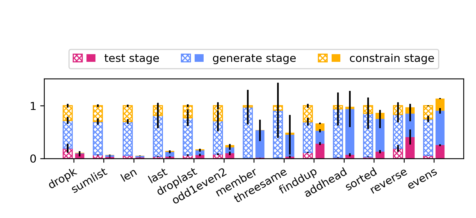
Figure 5 shows the relative time spent in each stage of Hempel and Popper. We can infer the overhead of failure explanation by analysing SLD-trees from this figure. All problems from odd1even2 to evens have Hempel spend more time on testing than Popper. On finddup, reverse and evens, Hempel incurs considerable testing overhead. While for finddup this effort translates into more effective pruning constraints, for sorted and evens this is not the case. Abstracting away from the implementation of failure explanation, we see that Popper outfitted with zero-overhead failing sub-program identification would have been strictly faster.
There is considerable variance in the number of generated programs and learning times on three problems. This is in large part due to the solver that is used, Clingo clingo, yielding models, i.e. hypotheses, non-deterministically. That is, there is no fixed order in which we see hypotheses, so, by chance, Hempel and Popper can come across a solution considerably sooner in one trial than in another. As a remedy for this variance, we re-run these three problems with their hypothesis spaces restricted to programs that are strictly smaller than solutions. In this setup, Hempel and Popper always terminate precisely at the point when they have shown that none of these hypotheses can be a solution. The results, which indeed have less variance, are in Table 2.
Table 3 shows the mean accuracy and learning times of Metagol and Aleph versus Hempel. Accuracy is below 67% for Aleph on all problems, which can be ascribed to Aleph struggling to learn recursive programs. Metagol cannot find solutions for problems which require arity-three predicates (unless given hand-crafted metarules), which is why ‘Not Applicable’ is listed for five problems. On another four problems, Metagol returns low accuracy hypotheses. Only on two problems does Metagol outperform Hempel. In general, Hempel is the more flexible system and outperforms Metagol and Aleph.
Overall, these results strongly suggest that the answer to questions Q1 and Q2 is yes.
6.3 Experiment 3: IGGP and Michalski trains
For the next experiment, we evaluate Hempel on problems where solutions are larger, either because they require many clauses or many literals in a clause. We consider two settings: classification in the form of Michalski train problems michalski:trains and inductive general game playing iggp. The problems in these two settings are sufficiently hard that solutions cannot always be found in a reasonable timeframe, hence we rely on Hempel’s anytime capabilities to return the best scoring hypothesis it was able to find upon a timeout.
Michalski train problems concern classifying a train as either eastbound or westbound. The features available for classifying a train’s heading are its cars and their features: if a car is long or short, how many wheels the car has, how many loads and which loads it is carrying, and, finally, whether the car’s roof is open, closed or flat. The target predicate, westbound/1, acts as our classifier and BK predicates allow for inspecting features of the trains to be classified. We consider the same 4 instances considered by Cropper dcc-aaai. An example of one of the higher quality hypotheses for the trains4 problem is:
Inductive General Game Playing concerns learning the rules of games from observations of these games being played. The goal is to synthesize a set of rules which are consistent with the traces generated by a game from the General Game Playing competition generalgameplaying. The four games we consider are: minimal-decay, rock, paper, scissors (rps), buttons and coins. In each case we learn the predicate next.
Settings & Systems
For the trains problems, we provide two dyadic predicates, has_car and has_load, and 17 monadic predicates which encode features of cars and loads. We provide the types of arguments as well as whether they are inputs or outputs to Hempel, Popper and Aleph. We allow up to four clauses, and within each clause six variables and up to six body literals. No recursion is allowed. For Metagol we provide the same metarules as in the previous experiment. For Aleph we limit the search nodes to 30000.
For the IGGP problems we provide the monadic, dyadic and triadic predicates that encode the actions and information available to advance the game to the next state. For example, for rps we look for a definition of next_score/3 given predicates true_score/3, succ/2, does/3, wins/2, beats/2, different/2.
Method
We use the same instances of the problems considered by Cropper dcc-aaai. The four trains problems represent progressively harder instances, with trains1 having a one clause six-literal solution and trains4 needing 26 literals over four clauses for an optimal solution. Each trains problem has a 1000 examples available, though the distribution between positive and negative varies between tasks. We follow Cropper in that “we randomly sample the examples and split them into 80/20 train/test partitions.” The four games are selected as representative instances of the larger IGGP dataset.
We measure learning time and predictive accuracy. We repeat each experiment 10 times and record the mean and standard error. We enforce a 300 second timeout.
| Number of programs | Learning time (sec) | Accuracy | ||||||
| Problem | Popper | Hempel | ratio | Popper | Hempel | ratio | Popper | Hempel |
| rps | 10648 38 | 250 13 | 0.02 | 96 2 | 25 1 | 0.26 | 100 0 | 100 0 |
| minimal-decay | 23171 1538 | 1904 76 | 0.08 | 300 0.0 | 41 2 | 0.14 | 94 0 | 100 0 |
| buttons | 8022 2265 | 1073 144 | 0.13 | 300 0.2 | 300 0.0 | 1.00 | 90 0 | 90 0 |
| coins | 9458 934 | 535 151 | 0.06 | 300 0.0 | 300 0.0 | 1.00 | 88 3 | 85 1 |
| trains1 | 28 0.0 | 20 0.3 | 0.72 | 1.0 0.0 | 3 0.0 | 2.99 | 100 0 | 100 0 |
| trains2 | 9410 6144 | 306 188 | 0.03 | 210 137 | 15 9 | 0.07 | 91 5 | 98 2 |
| trains4 | 11223 377 | 1176 25 | 0.10 | 300 0.0 | 300 0.0 | 1.00 | 78 2 | 89 1 |
| trains3 | 11278 594 | 1315 23 | 0.12 | 300 0.0 | 300 0.0 | 1.00 | 91 2 | 96 1 |
| Learning time (sec) | Accuracy | |||||
| Problem | Hempel | Aleph | Metagol | Hempel | Aleph | Metagol |
| rps | 25 1 | 4 0.1 | N/A | 100 0 | 100 0 | N/A |
| minimal-decay | 41 2 | 4 0.1 | 300 0 | 100 0 | 94 0 | 88 0 |
| buttons | 300 0 | 137 4 | 300 0 | 90 0 | 87 0 | 80 0 |
| coins | 300 0 | 300 0.0 | N/A | 85 1 | 82 0 | N/A |
| trains1 | 3 0.0 | 2 0.3 | 162 38 | 100 0 | 100 0 | 100 0 |
| trains2 | 15 9 | 1 0.1 | 218 126 | 98 2 | 100 0 | 85 6 |
| trains4 | 300 0 | 215 4 | 300 0 | 89 1 | 100 0 | 67 0 |
| trains3 | 300 0 | 18 0.9 | 300 0 | 96 1 | 100 0 | 20 0 |
Results
Table 4 includes the results for Hempel and Popper. For the IGGP problems, we have that Hempel times out on coins and buttons, while Popper additionally times out on minimal-decay. On rps and minimal-decay, Hempel is able to find a solution with 100% accuracy. Note how Hempel only required around 250 programs for finding a solution for rps while Popper required over 10.000 programs. For minimal-decay Hempel needs to consider almost 2000 programs before coming across a solution while Popper cannot find one within the time limit.
In Table 5 we see the performance of Metagol and Aleph versus Hempel on the IGGP problems. As Metagol’s metarules do not support arity-three predicates, we have that it is unable to find programs for rps and coins. On the other two problems, Metagol timeouts and hence achieves the default accuracy for these problems. On coins, both Hempel and Aleph achieve the default accuracy. On rps, Aleph does better than Hempel by virtue of its learning time, though Hempel still beats Metagol. On the three other games, Hempel does better than both Aleph and Metagol.
Referring back to Table 4, we see that Hempel outperforms Popper on the three more difficult trains problems. On trains1 we see clearly the overhead of failure explanation. Even though Hempel requires less programs than Popper, testing 800 examples incurs 800 times the linear overhead of failure explanation (with regards to SLD-tree size) plus the cost of retesting failing sub-programs, of which there are more when we are dealing with bigger hypotheses. On the other three problems, the cost of failure explanation is outweighed by the pruning it achieves, with Hempel finding more accurate solutions. Not shown in Table 4, for the timeouts, Hempel spends a greater proportional of time in the test-stage than Popper, e.g. about two-thirds of the time on trains4 versus just one-third of the time, respectively. This is likely attributable to the cost of retesting many sub-programs on the high number of examples.
From Table 5 we can see that Aleph’s bottom clause construction-based learning procedure is quite effective, outperforming Hempel on all four trains problems. In turn, Hempel outperforms Metagol on all trains problems.
Also for this experiment, the results indicate that the answer to questions Q1 and Q2 is yes, though with the note that larger hypotheses do appear to impact the effectiveness.
6.4 Experiment 4: string transformations
We now explore whether failure explanation can improve learning performance on real-world string transformation tasks. We hence restrict ourselves to comparing Hempel versus Popper. We use a standard dataset metabias; playgol formed of 312 tasks, each with 10 input-output pair examples. For example, task 81 has the following two input-output pairs:
| Input | Output |
|---|---|
| “Alex”,“M”,41,74,170 | M |
| “Carly”,“F”,32,70,155 | F |
Settings.
As background knowledge, we give each system the monadic predicates is_uppercase, is_empty, is_space, is_letter, is_number and dyadic predicates mk_uppercase, mk_lowercase, skip1, copyskip1, copy1. For each monadic predicate we also provide a predicate that is its negation. We allow up to 3 clauses, with each clauses having a maximum of 4 body literals and up to 5 variables. We extend the test stage with a check whether the generated program is functional or not and prune for any non-functional program.
Method.
The dataset has 10 positive examples for each problem. We perform cross validation by selecting 10 distinct subsets of 5 examples for each problem, using the other 5 to test. We measure learning times and number of programs generated. We enforce a timeout of 60 seconds per task. We repeat each experiment 10 times, once for each distinct subset, and record means and standard errors.
Results.
In 132 problems both Hempel and Popper return programs which have non-zero accuracy on the test set. On 64 tasks Hempel scores better than Popper versus Popper scoring better on 20 tasks. For 54 problems at least one of Popper and Hempel finds solutions with over 90% mean accuracy. Hempel finds solutions1010 10 Note that these problems are very difficult with many of them not having solutions given only our primitive BK and with the learned program restricted to defining a single predicate. Therefore, absolute performance should be ignored. The important result is the relative performance of the two systems. with 100% accuracy on 37 tasks, 3 more than Popper.
Figure 6 plots ratios of generated programs and learning times. Each of the 54 points represents a single problem where either Hempel or Popper scored over 90% mean accuracy. The x-axis is the ratio of number of programs that Hempel generates versus the number of programs that Popper generates. The y-value is the ratio of learning time of Hempel versus Popper. These ratios are acquired by dividing means, the mean of Hempel over that of Popper.
Looking at x-axis values, of the 54 problems plotted all require fewer programs when run with Hempel. Looking at the y-axis, the learning times of 51 problems are faster for Hempel.
Overall, these results show that, compared to Popper, Hempel typically needs fewer programs and less time to learn programs. This suggests that the answer to questions Q1 and Q2 is yes.
7 Conclusions
We introduced a method for using fine-grained failure explanation to derive fine-grained hypothesis space constraints. We illustrated this general method by a new SLD-based algorithm to identify failing sub-programs at the granularity of literals. We introduced an ILP system with failure explanation, Hempel, and experimentally showed that enabling failure explanation can drastically reduce hypothesis space exploration and learning times.
7.1 Limitations and future work
Application of sub-program based failure explanation is not restricted to fully automated program synthesis. For example, our SLD-based algorithm could be used for explainable AI purposes, e.g. in interactive environments such as tutor systems which help teach Prolog.
While not documented here, our approach works without modification in combination with an extension of Popper which supports predicate invention poppi. In an orthogonal direction, ILP noise handling methods could leverage failure explanation, e.g. by learning that the training error of a failing sub-program is as bad as the original program.
There are interesting theoretical questions to be worked out. As seen in Experiment 2, it appears that many smaller sub-programs are key to effective pruning. It should be possible to quantify the (theoretical) effectiveness of sub-program based pruning, e.g. with respect to the size of a sub-program and hypothesis space parameters such as the number of predicates. In general, future work should try to determine characteristics of problems that allow or preclude effective pruning based on failure explanation.
We require retesting of a sub-program derived from a hypothesis failing on a positive example to determine if this sub-program fails on the same example. This retesting is especially costly if there are many sub-programs, as is more likely to happen for bigger programs. Theoretical work is needed to identify cases where it follows from the original SLD-tree only having failing branches that the SLD-tree for the sub-program has no successful branch either. This would allow for eliding some of the expensive retesting that Hempel does.
Another major avenue for future work is leveraging fine-grained failure explanation for learning programs from logic fragments extending beyond definite programs. It should be possible to support negation-as-failure to a degree, e.g. by saying that clauses defining a predicate that occurred negated in a hypothesis are also responsible for a failure. Work on justifications for Answer Set Programming ASPjustifications could be used for fine-grained pruning whilst learning ASP programs.
Although we have shown that failure explanation can drastically reduce learning times, there is still much scope for improvement. For instance, Experiment 2 had the following failing sub-program occur:
Straightforward reasoning tells us literal head(A,D) is not relevant to the failure of this sub-program. Furthermore, we should be able to lay the blame on just the last two literals.
References
- [1] John Ahlgren and Shiu Yin Yuen. Efficient program synthesis using constraint satisfaction in inductive logic programming. JMLR, 2013.
- [2] Hendrik Blockeel and Luc De Raedt. Top-down induction of first-order logical decision trees. AIJ, 1998.
- [3] Alan Bundy and Boris Mitrovic. Reformation: A domain-independent algorithm for theory repair. Technical report, University of Edinburgh, 2016.
- [4] Rafael Caballero, Adrián Riesco, and Josep Silva. A survey of algorithmic debugging. ACM Comput. Surv., 2017.
- [5] James Cheney, Laura Chiticariu, and Wang Chiew Tan. Provenance in databases: Why, how, and where. Found. Trends Databases, 2009.
- [6] Andrew Cropper. Playgol: Learning programs through play. IJCAI, 2019.
- [7] Andrew Cropper. Learning logic programs through divide, constrain, and conquer. In AAAI, 2022.
- [8] Andrew Cropper, Richard Evans, and Mark Law. Inductive general game playing. Machine Learning, 2020.
- [9] Andrew Cropper and Rolf Morel. Learning programs by learning from failures. Machine Learning, 2021.
- [10] Andrew Cropper and Rolf Morel. Predicate invention by learning from failures. CoRR, abs/2104.14426, 2021.
- [11] Andrew Cropper and Stephen H. Muggleton. Metagol system. https://github.com/metagol/metagol, 2016.
- [12] Kevin Ellis, Lucas Morales, Mathias Sablé-Meyer, Armando Solar-Lezama, and Josh Tenenbaum. Learning libraries of subroutines for neurally-guided bayesian program induction. In NeurIPS, 2018.
- [13] Richard Evans and Edward Grefenstette. Learning explanatory rules from noisy data. JAIR, 2018.
- [14] Richard Evans, José Hernández-Orallo, Johannes Welbl, Pushmeet Kohli, and Marek Sergot. Making sense of sensory input. Artificial Intelligence, 2021.
- [15] Jorge Fandinno and Claudia Schulz. Answering the ”why” in answer set programming - A survey of explanation approaches. Theory Pract. Log. Program., 19(2):114–203, 2019.
- [16] Yu Feng, Ruben Martins, Osbert Bastani, and Isil Dillig. Program synthesis using conflict-driven learning. In PLDI, 2018.
- [17] Martin Gebser, Roland Kaminski, Benjamin Kaufmann, and Torsten Schaub. Clingo = ASP + control: Preliminary report. CoRR, abs/1405.3694, 2014.
- [18] Michael R. Genesereth and Michael Thielscher. General Game Playing. Synthesis Lectures on Artificial Intelligence and Machine Learning. Morgan & Claypool Publishers, 2014.
- [19] Céline Hocquette and Stephen H. Muggleton. Complete bottom-up predicate invention in meta-interpretive learning. In IJCAI, 2020.
- [20] Tobias Kaminski, Thomas Eiter, and Katsumi Inoue. Meta-interpretive learning using hex-programs. In IJCAI, 2019.
- [21] Frank C Keil and Robert Andrew Wilson. Explanation and cognition. MIT press, 2000.
- [22] Sven Köhler, Bertram Ludäscher, and Yannis Smaragdakis. Declarative datalog debugging for mere mortals. In Datalog in Academia and Industry, 2012.
- [23] J. Larson and Ryszard S. Michalski. Inductive inference of VL decision rules. SIGART Newsletter, 63:38–44, 1977.
- [24] Mark Law. Inductive learning of answer set programs. PhD thesis, Imperial College London, UK, 2018.
- [25] Mark Law, Alessandra Russo, Elisa Bertino, Krysia Broda, and Jorge Lobo. Fastlas: scalable inductive logic programming incorporating domain-specific optimisation criteria. In AAAI, 2020.
- [26] Dianhuan Lin, Eyal Dechter, Kevin Ellis, Joshua B. Tenenbaum, and Stephen Muggleton. Bias reformulation for one-shot function induction. In ECAI, 2014.
- [27] John W Lloyd. Foundations of logic programming. Springer Science & Business Media, 2012.
- [28] Herman Midelfart. A bounded search space of clausal theories. In ILP, 1999.
- [29] Stephen Muggleton. Inductive logic programming. New Generation Comput., 1991.
- [30] Stephen Muggleton. Inverse entailment and progol. New Generation Comput., 1995.
- [31] Shan-Hwei Nienhuys-Cheng and Ronald de Wolf. Foundations of Inductive Logic Programming. Springer-Verlag New York, Inc., Secaucus, NJ, USA, 1997.
- [32] Michael J Pazzani and Clifford A Brunk. Detecting and correcting errors in rule-based expert systems: an integration of empirical and explanation-based learning. Knowledge acquisition, 3(2):157–173, 1991.
- [33] G.D. Plotkin. Automatic Methods of Inductive Inference. PhD thesis, Edinburgh University, August 1971.
- [34] K.R. Popper. Conjectures and Refutations: The Growth of Scientific Knowledge. Routledge, 1963.
- [35] Luc De Raedt and Maurice Bruynooghe. Interactive concept-learning and constructive induction by analogy. Machine Learning, 1992.
- [36] Mukund Raghothaman, Jonathan Mendelson, David Zhao, Mayur Naik, and Bernhard Scholz. Provenance-guided synthesis of datalog programs. PACMPL, 2020.
- [37] Bradley L. Richards and Raymond J. Mooney. Automated refinement of first-order horn-clause domain theories. Mach. Learn., 19(2):95–131, 1995.
- [38] Peter Schüller and Mishal Benz. Best-effort inductive logic programming via fine-grained cost-based hypothesis generation. Machine Learning, 2018.
- [39] Ehud Y. Shapiro. Algorithmic Program DeBugging. MIT Press, Cambridge, MA, USA, 1983.
- [40] João P. Marques Silva, Inês Lynce, and Sharad Malik. Conflict-driven clause learning SAT solvers. In Handbook of Satisfiability. 2009.
- [41] Tom Silver, Kelsey R. Allen, Alex K. Lew, Leslie Pack Kaelbling, and Josh Tenenbaum. Few-shot bayesian imitation learning with logical program policies. In AAAI, 2020.
- [42] A. Srinivasan. The ALEPH manual. 2001.
- [43] George Thompson and Allison K. Sullivan. Profl: a fault localization framework for prolog. In ISSTA, 2020.
- [44] Stefan Wrobel. First order theory refinement. Advances in inductive logic programming, 32:14–33, 1996.
Appendix A Experiment 2: Metagol Settings
The following metarules were used for running Metagol in the programming puzzles experiment.
Appendix B Experiment 2: Hypothesis Space Settings
The following hypothesis space settings were used in the programming puzzles experiment:
| problem |
max #clauses |
max #literals |
max #variables |
sum/3 |
cons/3 |
snoc/3 |
head/2 |
tail/2 |
element/2 |
decrement/2 |
increment/2 |
qeg/2 |
even/1 |
odd/1 |
one/1 |
zero/1 |
empty/1 |
| addhead/2 | 3 | 7 | 6 | x | x | x | x | x | x | x | x | x | x | x | |||
| dropk/3 | 3 | 6 | 5 | x | x | x | x | x | x | x | x | x | x | x | x | ||
| droplast/2 | 3 | 6 | 5 | x | x | x | x | x | x | x | x | x | x | x | |||
| evens/1 | 2 | 6 | 5 | x | x | x | x | x | x | x | x | x | |||||
| finddup/2 | 2 | 6 | 5 | x | x | x | x | x | x | x | x | x | x | x | |||
| last/2 | 3 | 7 | 6 | x | x | x | x | x | x | x | x | ||||||
| len/2 | 2 | 6 | 6 | x | x | x | x | x | x | x | x | x | x | ||||
| member/2 | 3 | 7 | 6 | x | x | x | x | x | x | x | x | x | x | ||||
| odd1even2/2 | 3 | 6 | 5 | x | x | x | x | x | x | x | x | x | |||||
| reverse/2 | 3 | 5 | 5 | x | x | x | x | x | x | x | x | x | x | ||||
| sorted/1 | 3 | 6 | 5 | x | x | x | x | x | x | x | x | x | |||||
| sumlist/2 | 2 | 6 | 5 | x | x | x | x | x | x | x | x | x | x | x | |||
| threesame/1 | 3 | 7 | 6 | x | x | x | x | x | x | x | x | x | x |