Complexity Conjecture of Regular Electric Black Holes
Abstract
Recently, the action growth rate of a variety of four-dimensional regular magnetic black holes in frame is obtained in ElMoumni:2020nse. Here, we study the action growth rate of a four-dimensional regular electric black hole in frame that is the Legendre transformation of frame. We also investigate the action growth rates of the Wheeler-De Witt patch for such black hole configurations at the late time and examine the Lloyd bound on the rate of quantum computation. We show that although the form of the Lloyd bound formula remains unaltered, the energy modifies due to a non-vanishing trace of the energy-momentum tensor and some extra terms may appear in the total growth action. We also investigate the asymptotic behavior of complexity in two conjectures for static and rotating regular black holes.
I Introduction
AdS/CFT correspondence AdSCFT1; AdSCFT2; AdSCFT3 is a leading formalism providing a consistent relation between gauge and gravitation theories and has given us a rather deep insight on possible unification of them. Such a correspondence captures an equivalence between the conformal field theory and its dual theory of gravity in AdS space with a strong/weak duality point of view. It is believed that it provides a non-perturbative formulation access to strongly coupled regimes of quantum field theories which cannot be accessed by the traditional perturbation approach. Indeed, AdS/CFT correspondence is one of the important examples of entanglement between gravity and quantum information AdSCFT4; AdSCFT5; AdSCFT6; AdSCFT7. Complexity has recently been introduced as a complement to entanglement providing additional information on the quantum properties of black holes.
In order to calculate the holographic duality of quantum computational complexity one may follow two proposals. The (CV) A1; A2 and complexity = action (CA) B1; B2 conjectures. The former one states that the complexity of the boundary state is proportional to the maximum volume of codimension hypersurface bounded by the CFT slices and the latter conjecture specifies that complexity on the boundary CFT is proportional to the on-shell action of the Wheeler-DeWitt(WDW) patch in the bulk. According to these conjectures, Lloyd showed that the growth rate of complexity for the Schwarzschild like black holes is bounded by the total energy of the system Lloyd2000. Cai, et.al proved that the so-called Lloyd bound should be modified for charges or rotating black holes Cai2016. Although there are many cases of black holes that confirm the mentioned upper bound L1; L2; L3; L4; L5; L6; L7, its validity is an open question since there are different types of black hole violating the Lloyd bound V1; V2; V3. Accordingly, the validity of CV and CA conjectures and their possible modifications deserve further study.
In this direction, here, we focus on the holographic complexity of nonlinearly charged regular black holes in frame. Indeed, the motivation for studying this black hole is three folds: regularity, nonlinearity and complexity. The first item is the regularity of the black hole with known action, exactly. The second one is nonlinearity which has the key role to avoid the singularity. Although such a nonlinear electrodynamics is an ad hoc model near the black hole, it behaves like the Maxwell field far from the horizon radius. The third one is the complexity of black holes which is reasonable for regular black holes since the singularity may violate the interpretation of physical quantities such as entangled entropy and complexity.
The subject of singularity itself and its possible solution (leading to regularity) are highly interesting from different viewpoints: mathematical and geometrical points of view, classical gravity and its quantum standpoints, cosmological side, effective field theory and AdS/CFT correspondence features, string theory and supergravity aspects, etc. Indeed there are two important singularities that their natures are not yet fully understood: the singularity that is covered by an event horizon of black holes and the big bang singularity. So one of the substantial questions is how one can prevent the singularity. Although it is believed that quantum gravity can be able to smooth out singularities, there is no consistent theory of quantum gravity overcoming this issue despite many attempts. Thus, the question should again be asked how we can preclude the singularity in an alternative theory.
Regarding the Einstein theory of gravity coupling minimally with an appropriate nonlinear electrodynamics theory, various regular black hole metrics are constructed (for an incomplete list, please take a look at Balart2014; Ayon-Beato1998; Bronnikov2001; Arellano2006; Hassain2008; Hollenstein2008; Balart2009). The exact regular solution of gravity has been studied in Hollenstein2008. Gravitational lensing Eiroa:2010wm, dynamical Fernando:2012yw and thermodynamical stability Hendi:2020knv of regular black hole has been studied. A new Smarr-type formula for the black hole in nonlinear electrodynamics has been obtained in kastor09; Balart:2017dzt. In this paper, we concentrate on the complexity of a simple static and rotating regular black hole with nonlinear electrodynamics as a source. The rest of the paper is organized as follows. In Sec. II, we briefly review the complexity and thermodynamics of regular black hole, especially deriving its Smarr formula. Section III is devoted to study the complexity of large-extremal-static regular black hole in the framework of CA and CV conjectures and comparing the results in two frameworks. In Sec. IV, we repeated the same computation of complexity for the large-extremal rotating regular black holes. After that, conclusions are given. In the appendix, we also investigate two other regular cases and calculated thermodynamic quantities, complexity and complexity of formation numerically.
II basic formalism
Electrically charged black hole solutions can be studied through an alternative form of nonlinear electrodynamics obtained by the Legendre transformation. The action of nonlinear electrodynamics in frame minimally coupled to the Einstein gravity with the York-Gibbons-Hawking surface term and the two-dimensional joint term is given by
| (1) | |||||
where is the determinant of the metric, is the Ricci scalar and the negative cosmological constant is denoted by . In addition, the anti-symmetric tensor in which , and is the Faraday tensor. Furthermore, the structure function is with since , where . Moreover, and are, respectively, the determinant of the induced metrics in three-dimensions and two-dimensional . Also, is the trace of the extrinsic curvature of the induced metric
| (2) |
where is the normal vector. The integrant is defined as
in which is the future-directed null normal to the left-moving null surface and denotes the future-directed null normal to the right-moving null surface.
The first integral of Eq. (1) represents the bulk action while the second and third ones stand for the boundary and joint parts of the WDW patch Lehner:2016vdi. The WDW patch is used to obtain the rate of temporal change of the action. A typical WDW patch of a black hole with two horizons is shown in Fig. 4 which is evolved in time from to . According to this figure, the contribution of different parts is bulk region and , and null-null surface joints , , and (for more details, see Lehner:2016vdi). Hence, we can write
| (3) | |||||
where is the Lagrangian of Einstein-nonlinear electrodynamics. In order to compute the contribution of joints, we use the following transformation of and
| (4) |
in which and are two arbitrary positive constants and the tortoise coordinate is defined as . So, the contribution of joints is calculated as
| (5) |
| (6) |
where prime denotes derivative with respect to . In Fig. 1, we assume close cylindrical hypersurfaces consisting of a past spacelike surface , a truncated null cone , a future spacelike surface and boundaries for intersection of spacelike and null surfaces and .


The contribution of surfaces and canceled each other in Fig. (1a) due to the same direction of normal vectors. While for Fig. (1b) according to opposite direction of normal vectors, contributions of boundaries of intersection of surfaces, and cancel each other. Therefore depending on what we choose for direction of normal vector, boundary terms or joint contributions will be vanished Lehner:2016vdi.
It is notable that applying the variational principle to the action (1), one finds the field equations as
| (7) |
| (8) |
where is the Einstein tensor. By integrating equation (8) with the assumption of spherical symmetry spacetime, we obtain the following static solution
| (9) |
| (10) |
where is an integration constant and .
In the following, for the importance of Smarr relation, we will obtain it for the case of spherically symmetric static charged regular black holes. In order to do that we use the Komar formula for the mass of black holes as follows
| (11) |
where is a timelike Killing vector which satisfies Killing equation and is a two-dimensional surface element of the boundary at infinity. Since the spacetime has two boundaries, we will write the Komar integral for the mass as a sum of an integral over a closed null surface at the horizon and an integral on the spacelike hypersurface which is bounded by the horizon and infinity as
| (12) |
For the first term, we have
| (13) |
where is the horizons surface area, denotes the surface gravity that is constant at the event horizon and satisfies . In order to evaluate the second term in equation (12), we consider the Stokes theorem for an antisymmetric tensor field as follows
| (14) |
For the antisymmetric tensor of the bulk term , we have
| (15) |
where . Recalling that , we get
| (16) |
Now, by using the Einstein field equation , we obtain
| (17) |
On the other hand, considering equation (7), the nonzero components of energy-momentum tensor are
| (18) |
By rewriting the RHS of Eq. (17), one can obtain
| (19) |
since the timelike Killing vector is and with identically. Finally, by inserting above results in Eq. (12), we obtain
| (20) |
where is the trace of the induced metric of spacelike hypersurface.
III The complexity growth of regular electric black holes
Here, we consider a class of known regular electric black holes in AdS spacetime and calculate its complexity growth rate. For the sake of completeness, we will point out other regular black hole solutions in the appendix.

The motivations of considering the forthcoming kind of function are its simplicity and its agreement to the correspondence which indicates such a modified nonlinear theory should reduce to the usual Maxwell theory in the weak-field limit. The ansatz of structure function which is inspired by the exponential distribution is defined as Balart:2014cga
| (21) |
in which for the weak field limit (), it reduces to the Maxwell field as
| (22) |
Considering the mentioned structure function with Eqs. (10) and (9), we can find the following spherically symmetric exponentially black hole solution Balart:2014cga; Balart:2014jia; Culetu:2014lca; Hendi:2020knv; Ghosh:2014pba
| (23) |
Using the series expansion of this solution for large values of , it is noticeable that its asymptotical behavior can be found by the following expression
| (24) |
which is the Reissner-Nordström-AdS metric function provided and are associated with the mass and electric charge of the system, respectively. In other words, the asymptotical behavior of the obtained solution is completely matched to the Reissner-Nordström-AdS black hole.
In order to check the first law and the Smarr formula in the extended phase space, it is convenient to consider the cosmological constant as a varying thermodynamic quantity and interpret it as a thermodynamic pressure, as . In addition, its conjugate variable of the introduced pressure is the thermodynamic volume
| (25) |
where is the event horizon radius obtained via . The temperature would be found straightforwardly through the use of surface gravity () interpretation with the following explicit relation
| (26) |
in which for the large black hole event horizon () becomes
| (27) |
Since we are working in the Einstein gravity, the black hole entropy pursues the area law, yielding
| (28) |
In addition, the electrostatic potential can be obtained at the event horizon versus spatial infinity as the reference
| (29) |
and the asymptotic limit becomes
| (30) |
For a black hole embedded in AdS spacetime, employing the relation between the cosmological constant and thermodynamic pressure would result to interpret the mass of black hole as the enthalpy. The enthalpy can be written in terms of thermodynamic quantities as
| (31) |
where is the function. In the case of large black hole event horizon, we have
| (32) |
It is straightforward to check that these thermodynamic quantities satisfy the first law of black hole thermodynamics in the enthalpy representation
| (33) |
and the Smarr relation is given by
| (34) |
where the last term of Eq. (34) comes from the fact that the energy-momentum tensor is not traceless, as
| (35) |
and in the case of becomes
| (36) |

Now, we want to calculate the complexity growth rate in the above background. For this aim, we should calculate the Ricci scalar for the solution (23) as
| (37) |
whereas by using of Eq. (21), the Lagrangian of nonlinear electrodynamics is given by
| (38) |
Using Eqs. (37) and (38), we can calculate the bulk action growth as
| (39) |
while the growth rate of the surface term (Eq. (1)) is given by ElMoumni:2020nse
| (40) | |||||
where we should note that in the calculation of boundary term we have used and .
Besides, the contribution of joint terms can be calculated as
| (41) |
After some manipulations, we can find
| (42) | ||||
| (43) |
Since at the late time and approach to and , respectively, while vanishes, one finds Eqs. (42) and (43) reduce to
| (44) | |||||
| (45) |
So, the total growth rate of the action for such a black hole configuration within WDW patch at late time approximation is simplified as
| (46) |
In order to describe Eq. (46) in terms of and , we can use the redefinitions and in terms of and as
| (47) |
where
| (48) |
Although it is straightforward to rewrite Eq. (46) in terms of and , we ignore its explicit relation for the sake of brevity. Finally, by using the above calculated thermodynamic quantities, it is easy to show that
| (49) |
indicating that the action growth rate of the black hole in the WDW patch has been bounded. For instance, for the values this bound is about , and the differences between left and right (right mines left) is about which is clearly non-negative. It is worth mentioning that although there are some extra terms in the right hand side of Eq. (49) due to considering the nonlinear electrodynamics as a source, the action growth rate is bounded.
III.1 Extreme case:
Now, we focus on the extremal solutions. By introducing , and in the case of extremal, large black hole, equation (46) becomes
| (50) |
in terms of leads to
| (51) |
By using of equations (25), (32) and () one can rewrite above equation as follows Couch:2016exn
| (52) |
which shows that in the large black holes the rate of complexity is proportional to , i.e, is controlled by thermodynamical volume. Besides, it is notable that one can obtain such a relation in terms of entropy for the static black holes since in the static case the thermodynamic volume is not independent of entropy ().
In the case of extremal black hole with small degenerate horizon radius, we have
| (53) |
By using of CV conjecture, the rate of complexity is An:2018dbz
| (54) |
where is the turning point of maximal surface. The late time limit of becomes
| (55) |
where is the extreme value point of . For the present case we need to obtain the zeros of the following equation
| (56) |
in the case of small , it becomes
| (57) |
where
| (58) |
In the case of extremal black hole with large horizon radius, we can write
| (59) |
and correspondingly, for the late time of growth of complexity, we obtain
| (60) |
The comparison of the complexity growth from the CV and CA dualities are
| (61) |
III.2 Complexity of formation
The complexity of formation is the difference between complexity in the process of forming the entangled TFD state and preparing two individual copies of the vacuum state of the left and right boundary CFTs Chapman:2016hwi; Cottrell:2017ayj
| (62) |
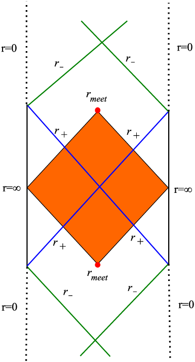
For the case of charged black hole with two horizons, the complexity of formation in CA conjecture becomes Chapman:2016hwi
| (63) |
Now, we evaluate the action for the obtained black hole solutions. The tortoise coordinate for the both horizons of the solution is
| (64) |
The point where the ingoing null rays from the two asymptotic regions meet inside the black hole between the two horizons () can be calculated numerically using Eqs. (64)-(136) which reads
| (65) |


We show the results for in Fig. 5 for the considered solution. According to the Fig. 5a, by increasing event horizon radius, decreases from extremal value to . Then, by increasing the electric charge, increases (Fig. 5b). By using of numerical curve fitting and choosing the appropriate branches of the logarithms, one can obtain the following relation for
| (66) |
The above approximation functions are necessary to obtain the and
in the following.
The bulk action of the black hole is
| (67) |
where is the constant defining the future null boundary, and is a some cutoff surface associated with a UV divergence. In order to obtain the action of AdS spacetime, one uses
| (68) |
in which the tortoise coordinate for AdS spacetime is
| (69) |
Thus the bulk action of AdS vacuum is
| (70) |
where and . Now, we should calculate the following relation for the solution
| (71) |
The action at the meet point is
| (72) |
which in the case of large black hole becomes
The total action is the sum of the bulk (71) and joint (72) terms. Substituting the numerical solution for , we obtain the interesting result plotted in Fig. 6. According to these figures, one finds the bulk action of black hole and complexity of formation are linear functions of entropy. For the large black hole, we have
| (73) |
where is the boundary central charge.


Here, we want to obtain the complexity of formation by using of CV conjecture. To do that, we consider the maximal volume functional for the timeslice (the straight line connecting the two boundaries through the bifurcation surface in the Penrose diagram) as follows Chapman:2016hwi; Balushi:2020wkt
| (74) |
where the corresponding contribution from two copies of the vacuum AdS background is
| (75) |
The complexity of formation is obtained by subtracting from (74) the volume of the AdS vacuum
| (76) |
To understand the behaviour of complexity of formation, we obtain the plot of as a function of in Fig. 6.
It is interesting, of course, to compare the results of CA and CV duality. The ratio of the complexity of formation for large black holes is
| (77) |
and by using (61) and (77) one gets
| (78) |
As can be seen, the differences between two ratios is small. So, the two ratios agree very well and this comparison suggests that the two holographic approaches to complexity are consistent.
IV Generalization to rotating solution:
The metric of rotating charged regular black hole in the Boyer-Lindquist coordinates is obtained as
| (79) |
where
| (80) |
The outer and inner horizons are determined by the equation , respectively. The required thermodynamical quantities to check the first law are Hendi:2020knv
| (81) |
where
| (82) |
So, the first law of thermodynamic is satisfied as Hendi:2020knv
| (83) |
Integrating the on-shell Einstein-Hilbert bulk action, directly, in the case of and leads to
| (84) |
since and
| (85) |
The growth rate of the surface term in the case of and (Eq. (1)) is
| (86) |
since the determinant of the induced metric on the null hypersurface is and the trace of extrinsic curvature can be calculated from Eq. (2) and the normal vector is . Combining the bulk action and boundary term, we can obtain the growth rate of total action as follows
| (87) |
where
In the case of , and , one finds
| (88) | |||||
while for , and , we have
| (89) | |||||
In addition, in the case of , and , we obtain
| (90) |
and for , and , one achieves
| (91) |
since
| (92) |
As can be seen in both cases , the rate of complexity proportional to the volume of black holes instead of entropy of black holes.
IV.1 Complexity of formation
In this section complexity of formation for rotating black holes in the limit and and in the conjectures Complexity-Action and Complexity-Volume is calculated.
To do so, we calculated Lagrangian of the bulk and vacuum AdS in the limit and , which in the second-order approximation are written the following form
For obtaining the complexity of formation we should compute the following relation:
where
Since and in the limit and can be calculated analytically, but the integral of the first term with respect to can not be calculated analytically thus it is actually more convenient to use integration by parts to eliminate the appearance of inside this expression, because after that we must integrating with respect to therefore the first integral must be calculated analytically,
is obtained in the same way. After some calculations complexity of formation for slowly rotating black holes in the limit within Complexity-Action conjecture is obtained which is shown in Fig. 7.

The behavior of () versus () is plotted in Fig. 8. We find that is approximately a linear function of event horizon and the best fitting curve relation is .


Complexity of formation in CV conjecture
For calculating the complexity in CV conjecture, we must find the surface with maximal volume. For this purpose we should write the line element in the tortoise coordinate
where
To find the maximal surface we describe the surface with the parametric relations and with some parameter , then the volume of the surface becomes in the following form
| (93) |
where dots indicate derivatives with respect to and the factor 2 is originated from this fact that the surface is composed from two equivalent parts. We are free to choose to keep the radial volume element fixed as follow
| (94) |
this Lagrangian is independent of and hence there is a conserved quantity given by
| (95) |
By substituting from (94) into the (95), one can obtain
with substituting above equations into the relation (93) for maximal surface volume one can find that
Here we wish to take to be infinity, but this will yield a divergent result in general. A finite result can be obtained by performing a carefully matched subtraction of the AdS vacuum. Here is the turning point of the surface which determined by the condition
A simple calculation shows that will be on or inside the (outer) horizon, and so we have that, , E and we recall that in the region between the inner and event horizon. We are interested in maximal slice which in this case which gives . Thus, the complexity of formation becomes
integrating with respect to gives us
As the next step, we have to integrate the above relation with respect to . In this case the integral cannot be calculated analytically, and therefore, we should calculate it numerically which the results are shown in Fig. 9.

According to Figs. 7 and 9, it is obvious that complexity of formation in two mentioned conjectures has same behavior and it is bounded without divergency. In the limit the value of the complexity of formation (calculated via CV conjecture) is reduced and tends to while at the large value of , it’s value approximately tends to a constant. Since increasing the electric charge leads decreasing (increasing) inner horizon (event horizon), it is easy to find that is an increasing function of electric charge, , and therefore, the complexity of formation in both conjectures increases as one increases the electric charge.
V Conclusion
In this paper, we studied the complexity of regular static and rotating black holes in the presence of nonlinear electrodynamics . For the case of the static black hole, by looking at the action growth rates of the Wheeler-De Witt patch, we showed the Lloyd bound is satisfied and its form remains unaltered . Then, we have obtained the rate of complexity and complexity of formation by using both CA and CV conjectures. From the comparison of the result, we concluded that the two approaches to the complexity are consistent. In the case of slowly rotating one and with assumption , we obtained the rate of complexity proportional to the volume of the black hole (in the limit and ). So, one can conclude that the rate of complexity for both static and rotating black holes is proportional to thermodynamical volume instead of entropy.
The complexity of formation is numerically obtained by using both conjectures. Its behavior is reflected in Figs. 7 and 9 which shows that for both conjectures, the complexity of formation has the same behavior and is bounded.
In the appendix, we investigated two other regular cases and obtained the rate of complexity and complexity of formation by using of both conjectures for them. According to Figs. 11 and 12, it is obvious that for each case, the complexity of formation obtained from two approaches are relatively consistent and on the other hand behavior of complexity of formation for these two regular cases have interesting similarities with each other.
Acknowledgements
The authors thank Shiraz University Research Council.
VI Appendix
For the sake of completeness, here, we investigate complexity conjecture of two more examples of static regular black holes in .
VI.1 Second Case:
Here, we consider another structure function inspired by the log-logistic distribution as the second class of solution which is given by Balart:2014cga; Dymnikova:2004zc
| (96) |
where , and and are two parameters. In the weak field limit (), Eq. (96) reduces to
| (97) |
Taking such a structure function into account with and Eqs. (10) and (9), we can, directly, achieve the following form of the solution Dymnikova:2004zc; Sajadi:2017glu
| (98) |
with the following asymptotical behavior for large
| (99) |
As a result, the obtained solution behaves like Reissner-Nordström-AdS, asymptotically, when we adjust and as the mass and electric charge of the system, respectively.
Such as before, we can obtain the following thermodynamic quantities for the recent solution
| (100) | |||||
| (101) | |||||
| (102) | |||||
| (103) | |||||
| (104) |
where . Having the mentioned thermodynamic quantities, one can directly examine the first law of black hole thermodynamics in the enthalpy representation
| (105) |
where
| (106) |
Moreover, the Smarr relation is given by
| (107) |
where
| (108) |
Now, we calculate joint terms according to joint contribution which is described in the first class. After simplification, we can write
| (109) |
Considering the metric function obtained here, it is easy to show that the Ricci scalar is calculated as
| (110) |
and also, the Lagrangian of nonlinear electrodynamics can be calculated at the event horizon with the following explicit form
| (111) |
Consequently, the growth rate of bulk action and surface term are, respectively,
| (112) |
and
| (113) |
Finally, we find that the total growth rate of the action for such black hole configuration within WDW patch at late time approximation can be collected as
| (114) |
Thus, by using the above calculated thermodynamic quantities, it is easy to show that the Lloyd bound is satisfied. As an example, for the values this bound is about , and the differences between left and right (right mines left of Eq. (49)) is about .
VI.2 Third Case:
As the third case, we consider the following structure function which is inspired by the Fermi-Dirac distribution functionAyonBeato:1999rg; Balart:2014cga
| (115) |
with the following weak field limit ()
| (116) |
Considering the spherically symmetric spacetime with previous relations for , the third class of solution is
| (117) |
According to the series expansion of the metric function for large , one can find this solution behaves like the Reissner-Nordström-AdS, asymptotically, as
| (118) |
whereas and will be associated with the mass and electric charge of the system, respectively.
Using the previous approach in the extended phase space, the following thermodynamical quantities can be obtained, directly,
| (119) | |||||
| (120) | |||||
| (121) | |||||
| (122) | |||||
| (123) |
It is evident that these thermodynamic quantities satisfy the first law of black hole thermodynamics as
| (124) |
where in the enthalpy representation, we have
| (125) |
In addition, the related Smarr formula is given by
| (126) |
where
| (127) |
According to the previous section, joint contribution can be calculated as below
| (128) |
| (129) |
Moreover, the Ricci scalar for this solution is simplified as
| (130) |
and the nonlinear Lagrangian is as follows
| (131) |
It is notable that the growth rate of the bulk action and its related surface term can be written as
| (132) | |||||
| (133) |
As a result, the total growth rate of action for such a black hole configuration within WDW patch at late time approximation is
| (134) |
For instance, for the values this bound is about , and the differences between left and right (right mines left of Eq. (49)) is .
VI.3 Complexity of formation
Similar to the complexity of formation of the first case we would like to study the complexity of formation of second and third cases. In this way, and of the second and the third solutions can be obtained as follows:
| (135) | ||||
| (136) |
and
| (137) | ||||
| (138) |
Accordingly, the bulk action of the black holes are
| (139) | ||||
| (140) |
here is the same as the first case. The relation for for large black holes are written in the following form:
| (141) | ||||
| (142) |

The figure of for second and third cases are plotted in Fig. 10. According to Fig. 10, it is obvious that for small black hole the contribution of the joints to the action is large for large black holes, this contribution becomes smaller and goes to zero.
Finally according to above relations and the results related to the spacetime (68)-(III.2), from (63) can be obtained. The plot of for second and third cases are shown in Fig. 11.
Figure 11 describes that complexity of formation for second and third cases increases for large black holes. Finally according to Eq. (76) for these two cases can be obtained.
Figure 12 shows that for both cases has the same behavior as with , increasing with radius of the black hole. To summarize the behavior of and for three cases versus are plotted in Fig. 13.


References
- (1) H. El Moumni and K. Masmar, Nucl. Phys. B 950, 114837 (2020).
- (2) G. ’t Hooft, Conf. Proc. C 930308, 284 (1993).
- (3) L. Susskind, J. Math. Phys. 36, 6377 (1995).
- (4) J. M. Maldacena, Int. J. Theor. Phys. 38, 1113 (1999) [Adv. Theor. Math. Phys. 2, 231 (1998)].
- (5) S. Ryu and T. Takayanagi, JHEP 08, 045 (2006).
- (6) V. E. Hubeny, M. Rangamani and T. Takayanagi, JHEP 07, 062 (2007).
- (7) H. Casini, M. Huerta, and R. C. Myers, JHEP 05, 036 (2011).
- (8) A. Lewkowycz and J. Maldacena, JHEP 08, 090 (2013).
- (9) L. Susskind, Fortsch. Phys. 64, 24 (2016).
- (10) D. Stanford and L. Susskind, Phys. Rev. D 90, 126007 (2014).
- (11) A. R. Brown, D. A. Roberts, L. Susskind, B. Swingle and Y. Zhao, Phys. Rev. Lett. 116, 191301 (2016).
- (12) A. R. Brown, D. A. Roberts, L. Susskind, B. Swingle and Y. Zhao, Phys. Rev. D 93, 086006 (2016).
- (13) S. Lloyd, Nature 406, 6799 (2000).
- (14) R. G. Cai, S. M. Ruan, S. J. Wang, R. Q. Yang and R. H. Peng, JHEP 09, 161 (2016).
- (15) W. J. Pan and Y. C. Huang, Phys. Rev. D 95, 126013 (2017).
- (16) P. A. Cano, R. A. Hennigar and H. Marrochio, Phys. Rev. Lett. 121, 121602 (2018).
- (17) A. Ovgun and K. Jusufi, [arXiv:1801.09615].
- (18) K. Meng, Eur. Phys. J. C 79, 984 (2019).
- (19) X. H. Feng and H. S. Liu, Eur. Phys. J. C 79, 40 (2019).
- (20) J. Jiang, Eur. Phys. J. C 79, 130 (2019).
- (21) J. Jiang, Phys. Rev. D 98, 086018 (2018).
- (22) E. Yaraie, H. Ghaffarnejad and M. Farsam, Eur. Phys. J. C 78, 967 (2018).
- (23) K. Nagasaki, Phys. Rev. D 98, 126014 (2018).
- (24) Z. Y. Fan and H. Z. Liang, Phys. Rev. D 100, 086016 (2019).
- (25) L. Balart and E. C. Vagenas, Phys. Rev. D 90, 124045 (2014).
- (26) E. Ayon-Beato and A. Garcia, Phys. Rev. Lett. 80, 5056 (1998).
- (27) K. A. Bronnikov, Phys. Rev. D 63, 044005 (2001).
- (28) A. V. B. Arellano and F. S. N. Lobo, Class. Quantum Grav. 23, 5811 (2006).
- (29) M. Hassain, Class. Quantum Grav. 25, 246 (2008).
- (30) L. Hollenstein and F. S. N. Lobo, Phys. Rev. D 78, 124007 (2008).
- (31) L. Balart, Mod. Phys. Lett. A 24, 2777 (2009).
- (32) E. F. Eiroa and C. M. Sendra, Class. Quant. Grav. 28, 085008 (2011).
- (33) S. Fernando and J. Correa, Phys. Rev. D 86, 064039 (2012).
- (34) S. H. Hendi, S. N. Sajadi and M. Khademi, [arXiv:2006.11575].
- (35) D. Kastor, S. Ray and J. Traschen, Class. Quant. Grav. 27, 235014 (2010).
- (36) L. Balart and S. Fernando, Mod. Phys. Lett. A 32, 1750219 (2017).
- (37) L. Lehner, R. C. Myers, E. Poisson and R. D. Sorkin, Phys. Rev. D 94, 084046 (2016).
- (38) L. Balart and E. C. Vagenas, Phys. Rev. D 90, 124045 (2014).
- (39) L. Balart and E. C. Vagenas, Phys. Lett. B 730, 14 (2014).
- (40) H. Culetu, Int. J. Theor. Phys. 54, 2855 (2015).
- (41) S. G. Ghosh, Eur. Phys. J. C 75, 532 (2015).
- (42) J. Couch, W. Fischler and P. H. Nguyen, JHEP 03, 119 (2017).
- (43) Y. S. An, R. G. Cai and Y. Peng, Phys. Rev. D 98, 106013 (2018).
- (44) S. Chapman, H. Marrochio and R. C. Myers, JHEP 01, 062 (2017).
- (45) W. Cottrell and M. Montero, JHEP 02, 039 (2018).
- (46) A. A. Balushi, R. A. Hennigar, H. K. Kunduri and R. B. Mann, [arXiv:2008.09138].
- (47) I. Dymnikova, Class. Quant. Grav. 21, 4417 (2004).
- (48) S. N. Sajadi and N. Riazi, Gen. Rel. Grav. 49, 45 (2017).
- (49) E. Ayon-Beato and A. Garcia, Phys. Lett. B 464, 25 (1999).