跳到论文正文
W Papers独立论文阅读器 arXiv:2102.12512 论文正文 计算阅读时间 · 0%
引用这篇论文根据当前论文元数据生成,正式投稿前建议核对。


License: arXiv.org perpetual non-exclusive license
arXiv:2102.12512v2 [quant-ph] 20 Aug 2021

Symmetric distinguishability as a quantum resource

Robert SalzmannNilanjana Datta11footnotemark: 1 Thanks: University of Cambridge, Department of Applied Mathematics and Theoretical Physics, Wilberforce Road, Cambridge CB3 0WA, United Kingdom    Gilad Gour Xin Wang Thanks: Department of Mathematics and Statistics, University of Calgary, Alberta, Canada T2N 1N4 Thanks: Institute for Quantum Science and Technology, University of Calgary, Alberta, Canada T2N 1N4 Thanks: Institute for Quantum Computing, Baidu Research, Beijing 100193, China    Mark M. Wilde Thanks: Hearne Institute for Theoretical Physics, Department of Physics and Astronomy, and Center for Computation and Technology, Louisiana State University, Baton Rouge, Louisiana 70803, USA Thanks: Stanford Institute for Theoretical Physics, Stanford University, Stanford, California 94305, USA
Abstract

We develop a resource theory of symmetric distinguishability, the fundamental objects of which are elementary quantum information sources, i.e., sources that emit one of two possible quantum states with given prior probabilities. Such a source can be represented by a classical-quantum state of a composite system X​AXA, corresponding to an ensemble of two quantum states, with XX being classical and AA being quantum. We study the resource theory for two different classes of free operations: (i)(i) CPTPA{\rm{CPTP}}_{A}, which consists of quantum channels acting only on AA, and (i​i)(ii) conditional doubly stochastic (CDS) maps acting on X​AXA. We introduce the notion of symmetric distinguishability of an elementary source and prove that it is a monotone under both these classes of free operations. We study the tasks of distillation and dilution of symmetric distinguishability, both in the one-shot and asymptotic regimes. We prove that in the asymptotic regime, the optimal rate of converting one elementary source to another is equal to the ratio of their quantum Chernoff divergences, under both these classes of free operations. This imparts a new operational interpretation to the quantum Chernoff divergence. We also obtain interesting operational interpretations of the Thompson metric, in the context of the dilution of symmetric distinguishability.

1 Introduction

Distinguishability plays a central role in all of modern science. The ability to distinguish one possibility from another allows for making inferences from experimental data and making decisions based on these inferences or developing new theories. Thus, it is essential to understand distinguishability from a fundamental perspective. Furthermore, distinguishability is a resource, in the sense that fewer trials of an experiment are needed to arrive at conclusions when two different possibilities are more distinguishable from one another.

In this paper, we adopt a resource-theoretic approach to distinguishability in quantum mechanics that ultimately is helpful in and enriches our fundamental understanding of distinguishability. We note here that, more generally, the resource-theoretic approach to quantum information processing [CG19] has illuminated not only quantum information science but also other areas of research in physics and mathematical statistics. Our work differs from prior developments with a related motivation [Mat10, WW19a, WW19b], in that here we focus instead on what we call symmetric distinguishability, or alternatively, the Bayesian approach to distinguishability. The outcome of our efforts is a resource theory with a plethora of appealing features, including asymptotic reversibility with the optimal conversion rate being given by a ratio of Chernoff divergences. We explain these concepts in more detail in what follows. Our theory is similar in spirit to that proposed previously in [Mor09], but there are some notable differences and our conclusions are arguably stronger than those presented in [Mor09]. We refer to the resource theory that we propose here as the resource theory of symmetric distinguishability (RTSD).

1.1 Overview of the resource theory of symmetric distinguishability

The basic objects of this resource theory are elementary quantum information sources, which emit one of two quantum states with certain prior probabilities (i.e., the source emits a state ρ0\rho_{0} with probability pp or a state ρ1\rho_{1} with probability 1−p1-p). Such a source can be represented by the following classical–quantum (c-q) state:

ρX​A≔p⁡|0⟩​⟨0|⊗ρ0+(1−p)​|1⟩​⟨1|⊗ρ1,\rho_{XA}\coloneqq p|0\rangle\!\langle 0|\otimes\rho_{0}+\left(1-p\right)|1\rangle\!\langle 1|\otimes\rho_{1}, (1.1)

where p∈[0,1]p\in\left[0,1\right] is a prior probability and ρ0\rho_{0} and ρ1\rho_{1} are quantum states11 1 Throughout this paper we restrict attention for the most part to c-q states of the form in (1.1).. Note that the classical system is equivalently specified by a random variable that we also denote as XX. In analogy with the notation used in the resource theory of asymmetric distinguishability [WW19a, WW19b], it can be equivalently represented by a quantum box given by the triple (p,ρ0,ρ1)(p,\rho_{0},\rho_{1}). The nomenclature “box” is used here to indicate that a quantum system is prepared in the state ρ0\rho_{0} with probability pp and ρ1\rho_{1} with probability 1−p1-p and it is not known which is the case (thus, the system is analogous to an unopened box).

An important goal of the resource theory is to transform a state of the above form to the following state

σX​B≔q⁡|0⟩​⟨0|⊗σ0+(1−q)​|1⟩​⟨1|⊗σ1,\sigma_{XB}\coloneqq q|0\rangle\!\langle 0|\otimes\sigma_{0}+\left(1-q\right)|1\rangle\!\langle 1|\otimes\sigma_{1}, (1.2)

via a chosen set of free operations, where q∈[0,1]q\in\left[0,1\right] and σ0\sigma_{0} and σ1\sigma_{1} are quantum states. Note that the target system BB need not be isomorphic to the initial system AA. This corresponds to the following transformation between boxes: (p,ρ0,ρ1)↦(q,σ0,σ1)(p,\rho_{0},\rho_{1})\mapsto(q,\sigma_{0},\sigma_{1}). Note that in what follows, we often suppress the subscripts denoting the quantum systems, for notational simplicity.

Given such an elementary quantum source ρX​A≡(p,ρ0,ρ1)\rho_{XA}\equiv(p,\rho_{0},\rho_{1}), a natural way to study distinguishability is to consider the binary hypothesis testing task of discriminating between the states ρ0\rho_{0} and ρ1\rho_{1}. There are two possible errors that can be incurred in the process, namely, the type I error (mistaking ρ0\rho_{0} to be ρ1\rho_{1}) and the type II error (mistaking ρ1\rho_{1} to be ρ0\rho_{0}). In the setting of asymmetric hypothesis testing, one minimizes the type II error probability under the constraint that the type I error probability is below a given threshold. In contrast, in symmetric hypothesis testing, the two error probabilities are considered on the same footing and weighted by the prior distribution. The latter (also known as Bayesian discrimination) is arguably the first problem ever considered in the field of quantum information theory and solved in the single-copy case by Helstrom [Hel67, Hel69] and Holevo [Hol72]. The operational quantity in this task is the minimum (average) error probability, which we formally define in (3.2) and denote as perr​(ρX​A)p_{\operatorname{err}}(\rho_{XA}).

Let ρX​A(n)\rho_{XA}^{(n)} denote the c-q state corresponding to a source that emits the state ρ0⊗n\rho_{0}^{\otimes n} (resp. ρ1⊗n\rho_{1}^{\otimes n}) with probability pp (resp. (1−p)(1-p)). It is known that perr​(ρX​A(n))p_{\operatorname{err}}(\rho_{XA}^{(n)}) decays exponentially in nn, with exponent given by the Chernoff divergence (also known as the quantum Chernoff bound) of the states ρ0\rho_{0} and ρ1\rho_{1} [NS09, ACMnT+07]. Just as the resource theory of asymmetric distinguishability (RTAD) provides a resource-theoretic perspective to asymmetric hypothesis testing [Mat10, Mat11, WW19a], our resource theory (RTSD) provides a resource-theoretic framework for symmetric hypothesis testing. By the quantum Stein’s lemma, the relevant operational quantity in asymmetric hypothesis testing is known to be characterized by the quantum relative entropy [HP91, ON00], and in the RTAD, the optimal rate of transformation between quantum boxes was proved to be given by a ratio of quantum relative entropies [WW19a] (see also [BST19] in this context). In analogy and given the result of [ACMnT+07], it is natural to expect that, in the RTSD, the corresponding optimal asymptotic rate of transformation between quantum boxes is given by a ratio of Chernoff divergences. It is pleasing to see that this is indeed the case. In contrast, in [Mor09], only one-shot transformations are considered and hence, in contrast to our work, asymptotic transformations are not studied.

We consider the RTSD for two different choices of free operations: (i)(i) local quantum channels (i.e., linear, completely positive, trace-preserving maps) acting on the system AA alone, and (i​i)(ii) the more general class of conditional doubly stochastic (CDS) maps. We denote the former class of free operations by CPTPA{\rm CPTP}_{A}. A CDS map acting on a c-q state ρX​A\rho_{XA} defined through (1.1) consists of quantum operations acting on the system AA and associated permutations of the letters x∈𝒳x\in{\mathcal{X}}. A detailed justification behind the choice of CDS maps as free operations is given in Section 2, where the RTSD is introduced via an axiomatic approach.

In any quantum resource theory, there are several pertinent questions to address. What are the conditions for the feasibility of transforming a source state to a target state? If one cannot perform a transformation exactly, how well can one do so approximately? What is an appropriate measure for approximation when converting a source state to a target state? Is there a “golden unit” resource that one can go through as an intermediate step when converting a source state to a target state? At what rate can one convert repetitions (i.e., multiple copies) of a source state to repetitions of a target state, either exactly or approximately? More specifically, at what rate can one distill repetitions of a source state to the golden unit resource, either exactly or approximately? Conversely, at what rate can one dilute the golden unit resource to repetitions of a target state? Is the resource theory asymptotically reversible? In this paper, we address all of these questions within the context of the RTSD.

Given an elementary quantum source ρX​A\rho_{XA}, a natural measure of symmetric distinguishability is given by the minimum error probability perr​(ρX​A)p_{\operatorname{err}}(\rho_{XA}) in the context of Bayesian state discrimination (mentioned above). Then

SD⁡(ρX​A)≔−log⁡(2​perr​(ρX​A)){\rm{SD}}(\rho_{XA})\coloneqq-\log\left(2p_{\operatorname{err}}(\rho_{XA})\right) (1.3)

is a natural measure of the symmetric distinguishability (SD) contained in ρX​A\rho_{XA}.22 2 Note, however, that this measure is not unique and it is possible to define other measures. In this paper, logarithms are taken to base 22. A justification of this choice arises from the consideration of free states and infinite-resource states. For a detailed discussion of the notion of symmetric distinguishability in a more general setting, see Section 2. A natural choice of a free state for this resource theory is a c-q state of the form (1.1), for which p=1/2p=1/2 and ρ0\rho_{0} and ρ1\rho_{1} are identical and hence indistinguishable. For such a state, perr​(ρX​A)=1/2p_{\operatorname{err}}(\rho_{XA})=1/2, which is achieved by random guessing, and hence SD⁡(ρX​A)=0{\rm{SD}}(\rho_{XA})=0. Note that the converse is true also (i.e., SD⁡(ρX​A)=0{\rm{SD}}(\rho_{XA})=0 implies that ρ0\rho_{0} and ρ1\rho_{1} are identical and p=1/2p=1/2). Hence our choice of SD respects the requirement that a state has zero SD if and only if it is free. On the other hand, a natural choice of an infinite-resource state is a c-q state of the form (1.1), for which ρ0\rho_{0} and ρ1\rho_{1} have mutually orthogonal supports. This corresponds to an elementary quantum information source that emits perfectly distinguishable states. For such a state, perr​(ρX​A)=0p_{\operatorname{err}}(\rho_{XA})=0 and hence SD⁡(ρX​A)=+∞{\rm{SD}}(\rho_{XA})=+\infty. Thus our choice of SD validates the identification of such states as infinite-resource states.

An infinite-resource state has the desirable property that it can be converted to any other c-q state via CDS maps. Under CPTPA{\rm{CPTP}}_{A}, it can be transformed to any other c-q state with the same prior. Moreover, any given c-q state cannot be transformed to an infinite-resource state unless it is itself an infinite-resource state.

We coin the word SD-bit to refer to the unit of symmetric distinguishability, the basic currency of this resource theory. In fact, for every positive real number m≥0m\geq 0, it is useful to identify a family of c-q states that have mm SD-bits. In Definition 3.4 of Section 3.1, we consider a natural choice for such a family of c-q states. They are parametrized by M≡2mM\equiv 2^{m} and denoted as γX​Q(M)\gamma_{XQ}^{(M)}. Such a state, which we call an MM-golden unit, has the following key property: perr​(γX​Q(M))=12​Mp_{\operatorname{err}}(\gamma_{XQ}^{(M)})=\frac{1}{2M} and hence SD⁡(γX​Q(M))=log⁡M=m{\rm{SD}}(\gamma_{XQ}^{(M)})=\log M=m.

Consideration of an MM-golden unit also leads naturally to a clear definition of the fundamental tasks of distillation and dilution in the RTSD as the conversions of a given c-q state to and from, respectively, an MM-golden unit under free operations33 3 [Mor09] also considers transformations to and from a certain unit of resource. However, instead of the MM-golden unit that we consider, there the unit of resource is a dbit, which is a pair of orthogonal states and therefore corresponds to the case M=∞M=\infty of our golden unit. The advantage of our choice (MM-golden unit) is that it yields a more refined analysis also in the case of finite resources.. The previously mentioned task of transformations between two arbitrary c-q states under free operations can be achieved by first distilling an MM-golden unit (for the maximal possible MM) from the initial state and then diluting the distilled MM-golden unit to the desired target state. This is discussed in detail in Sections 4 and 5.

One fundamental setting of interest is the one-shot setting, with the question being to determine the minimum error in converting an initial source to a target source. We prove that this minimum error can be calculated by means of a semi-definite program. Thus, we can efficiently calculate this error in time polynomial in the dimensions of the AA and A′A^{\prime} systems.

Moving on to the case of asymptotic transformations, we consider the following fundamental conversion task via free operations:

ρX​A(n)≡(p,ρ0⊗n,ρ1⊗n)↦σX​B(m)≡(q,σ0⊗m,σ1⊗m),\displaystyle\rho_{XA}^{(n)}\equiv(p,\rho_{0}^{\otimes n},\rho_{1}^{\otimes n})\mapsto\sigma_{XB}^{(m)}\equiv(q,\sigma_{0}^{\otimes m},\sigma_{1}^{\otimes m}), (1.4)

where p,q∈[0,1]p,q\in[0,1] and, for i∈{0,1}i\in\{0,1\}, ρi\rho_{i} and σi\sigma_{i} are states of quantum systems AA and BB, respectively. The goal here is, for a fixed nn, to make mm as large as possible, and to evaluate the optimal asymptotic rate mn\frac{m}{n} of the transformation in the limit as nn becomes arbitrarily large. We allow for approximations in the transformation and require the approximation error to vanish in the asymptotic limit (n→∞n\to\infty). This approximation error will be measured with respect to an error measure (defined for c-q states of the form considered in this paper) that we denote by the symbol D′D^{\prime}. The precise definition of D′D^{\prime} and its mathematical properties are given in Section 3.2.

1.2 Main results

In this paper, we develop a consistent and systematic resource theory of symmetric distinguishability that answers the most important questions associated with a resource theory. In brief, the main contributions of this paper can be summarized as follows. In the following, all c-q states are assumed to be of the form (1.1), and they hence represent elementary quantum information sources.

  • •

    We define two new examples of generalized divergences, each of which satisfies the data-processing inequality (DPI). These are denoted as ξmin\xi_{\min} and ξmax\xi_{\max}. Moreover, we define a quantity, denoted as ξmax⋆\xi_{\max}^{\star}, on c-q states of the form (1.1), and we prove that it satisfies monotonicity under CDS maps.

  • •

    All of the above quantities are of operational significance in the RTSD:

    • –

      The one-shot exact distillable-SD of ρX​A\rho_{XA} under CPTPA{\rm{CPTP}}_{A} maps is given by ξmin​(ρX​A)\xi_{\min}(\rho_{XA}) (Theorem 4.3);

    • –

      The one-shot exact SD-cost of ρX​A\rho_{XA} under CPTPA{\rm{CPTP}}_{A} maps is given by ξmax​(ρX​A)\xi_{\max}(\rho_{XA}) (Theorem 5.3);

    • –

      The one-shot exact distillable-SD of ρX​A\rho_{XA} under CDS{\rm{CDS}} maps is given by its symmetric distinguishability, SD⁡(ρX​A){\rm{SD}}(\rho_{XA}) (Theorem 4.5);

    • –

      In addition, the one-shot exact SD-cost of ρX​A\rho_{XA} under CDS maps is given by ξmax⋆​(ρX​A)\xi_{\max}^{\star}(\rho_{XA}) (Theorem 5.5).

  • •

    ξmax​(ρX​A)\xi_{\max}(\rho_{XA}) and ξmax⋆​(ρX​A)\xi_{\max}^{\star}(\rho_{XA}) are both defined in terms of the Thompson metric of the state ρX​A{\rho_{XA}} (see Theorems 5.3 and 5.5), thus providing operational interpretations of the latter in the context of the RTSD44 4 Even though the Thompson metric has been widely studied in the mathematics literature, to the best of our knowledge, this is the first time an operational meaning has been given to it..

  • •

    The optimal asymptotic rate of exact and approximate SD-distillation for a state ρX​A≡(p,ρ0,ρ1)\rho_{XA}\equiv(p,\rho_{0},\rho_{1}), under both CPTPA{\rm{CPTP}}_{A} and CDS maps, is equal to its quantum Chernoff divergence, ξ⁡(ρ0,ρ1)\xi(\rho_{0},\rho_{1}) (Theorem 4.7 and 4.18), where

    ξ⁡(ρ0,ρ1)≔sups∈[0,1](−log⁡Tr⁡[ρ0s​ρ11−s]).\xi(\rho_{0},\rho_{1})\coloneqq\sup_{s\in\left[0,1\right]}\left(-\log\operatorname{Tr}[\rho_{0}^{s}\rho_{1}^{1-s}]\right). (1.5)
  • •

    The optimal asymptotic rate of exact SD-dilution for a state ρX​A\rho_{XA} is equal to its Thompson metric (see Theorem 5.12). This provides another clear operational interpretation for the latter.

  • •

    The optimal asymptotic rate of approximate SD-dilution for a state ρX​A\rho_{XA} is equal to its quantum Chernoff divergence (see Theorem 5.13).

  • •

    The optimal asymptotic rate of transforming one c-q state to another, under both CPTPA{\rm{CPTP}}_{A} and CDS{\rm{CDS}} maps, is equal to the ratio of their quantum Chernoff divergences (see Theorem 7.4). This result constitutes a novel operational interpretation of the Chernoff divergence beyond that reported in earlier work on symmetric quantum hypothesis testing [NS09, ACMnT+07]. It also demonstrates that the resource theory of symmetric distinguishability (RTSD) is asymptotically reversible.

In the following sections, we develop all of the above claims in more detail. In particular, in Section 2, we introduce a general resource theory of symmetric distinguishability, for arbitrary quantum information sources (given by an ensemble {px,ρx}x∈𝒳\{p_{x},\rho_{x}\}_{x\in{\cal X}} of quantum states), via an axiomatic approach. The resource theory studied in the rest of the paper is a special case of the above, namely, the one for elementary quantum information sources (i.e., corresponding to the choice |𝒳|=2|{\cal X}|=2). Certain necessary ingredients of the RTSD are introduced in this section and in Section 3. These include the notion of golden units, which facilitates a study of distillation and dilution of symmetric distinguishability (SD). SD-distillation and SD-dilution are studied in Sections 4 and 5, respectively, both in the one-shot and asymptotic regimes. In Section 6, we elucidate the salient features of the RTSD for certain examples of elementary quantum information sources. The interesting task of converting one elementary quantum information source to another via free operations is studied in Section 7. We conclude the main part of the paper with a summary and some open questions for future research. Various relevant quantities of the RTSD can be formulated as semi-definite programs (SDPs). These are stated in Sections 3 and 4, but some of their proofs appear in the appendices.

2 An axiomatic approach to the resource theory of symmetric distinguishability

In this section, we introduce an axiomatic approach to a resource theory of symmetric distinguishability, from which the particular resource theory that we study in this paper arises as a natural special case, corresponding to the choice |X|≡|𝒳|=2|X|\equiv|\mathcal{X}|=2 in what follows.

Consider an ensemble {px,ρx}x∈𝒳\{p_{x},\rho_{x}\}_{x\in\mathcal{X}} of quantum states. Such an ensemble can be described by a c-q state

ρX​A=∑x∈𝒳px​|x⟩​⟨x|⊗ρx.\rho_{XA}=\sum_{x\in\mathcal{X}}p_{x}|x\rangle\!\langle x|\otimes\rho_{x}\;. (2.1)

There are many functions that can be used to quantify the distinguishability of the ensemble of states above. Perhaps the function that is most operationally motivated is the guessing probability:

pguess​(X|A)\displaystyle p_{\rm{guess}}(X|A) ≔max⁡∑x∈𝒳{Λx}x∈𝒳⁡px​Tr​(Λx​ρx),\displaystyle\coloneqq\max_{\{\Lambda_{x}\}_{x\in{\cal X}}}\sum_{x\in{\cal X}}p_{x}\mathrm{Tr}(\Lambda_{x}\rho_{x}), (2.2)

where the maximum is over every possible POVM {Λx}x∈𝒳\{\Lambda_{x}\}_{x\in{\cal X}}.

We are interested in a notion of ensemble distinguishability that takes into account the prior distribution {px}x∈𝒳\{p_{x}\}_{x\in\mathcal{X}}, while distinguishing between the states in the ensemble, as opposed to state distinguishability, which is concerned only with the distinguishability of the states in the set {ρx}x∈𝒳\{\rho_{x}\}_{x\in\mathcal{X}}.

Motivated by the guessing probability and symmetric hypothesis testing, we identify an ensemble as free in the resource theory of symmetric distinguishability if the guessing probability takes on its minimum value; i.e., if the guessing probability is equal to 1|𝒳|\frac{1}{|\mathcal{X}|}, which is the same value attained by a random guessing strategy. Note that the guessing probability is equal to 1|𝒳|\frac{1}{|\mathcal{X}|} if and only if all the states of the ensemble {px,ρx}x∈𝒳\{p_{x},\rho_{x}\}_{x\in{\cal X}} are identical and the prior distribution is uniform. For the sake of completeness, we include a proof of this fact at the end of this section (see Lemma 2.6 below).

Thus, for all such ensembles, the symmetric distinguishability is equal to zero. The corresponding c-q state ρX​A=πX⊗ωA\rho_{XA}=\pi_{X}\otimes\omega_{A}, where πX≔IX/|𝒳|\pi_{X}\coloneqq{I_{X}}/{|{\cal X}|} is the completely mixed state, is then a ‘free’ state of the resource theory of symmetric distinguishability because it has zero SD. This leads us to identify the set of free states in the resource theory of symmetric distinguishability as follows:

𝔉⁡(X​A)≔{πX⊗ωA:ωA∈𝒟⁡(A)}.\mathfrak{F}(XA)\coloneqq\left\{\pi_{X}\otimes\omega_{A}:\omega_{A}\in\mathcal{D}(A)\right\}\;. (2.3)

Note that, in the above, we use the notation 𝒟⁡(A)\mathcal{D}(A) to denote the set of quantum states (i.e., density matrices) of the quantum system AA.

To make the notion of symmetric distinguishability (SD) precise, we introduce an axiomatic approach. Here, we define a preorder relation ≺\prec on the set of all c-q states, which satisfies Axioms I-V below (see Definition 2.1). We say a c-q state ρX​A\rho_{XA} has less symmetric distinguishability than σX′​A′\sigma_{X^{\prime}A^{\prime}} if ρX​A≺σX′​A′\rho_{XA}\prec\sigma_{X^{\prime}A^{\prime}}. In this approach, SD is a property of a composite physical system shared between two parties, say, Xiao and Alice, with Xiao possessing classical systems (denoted by XX, X′X^{\prime}, etc.) and Alice possessing quantum systems denoted by AA, A′A^{\prime}, etc. The word “symmetric” refers to the fact that the distinguishability is symmetric with respect to the ordering in the ensemble; i.e., for every permutation π\pi, the ensemble {px,ρx}x\{p_{x},\rho_{x}\}_{x} has the same SD as the ensemble {pπ⁡(x),ρπ⁡(x)}x\{p_{\pi(x)},\rho_{\pi(x)}\}_{x} because the latter is just a relabeling of the former. We write this equivalence as the following relation:

    Axiom I ρX​A∼𝒫X→X​(ρX​A)∀𝒫−permutation channel.\displaystyle\quad\rho_{XA}\sim\mathcal{P}_{X\to X}\!\left(\rho_{XA}\right)\quad\quad\forall\;\mathcal{P}-\text{permutation channel}. (2.4)

Similarly, every isometric channel 𝒱∈CPTP⁡(A→A′)\mathcal{V}\in{\rm CPTP}(A\to A^{\prime}) that acts on the states {ρx}x\{\rho_{x}\}_{x} does not change their “overlap” (i.e., their Hilbert–Schmidt inner product), and this leads to the next axiom:

    Axiom II ρX​A∼𝒱A→A′​(ρX​A)∀𝒱−isometric channel.\displaystyle\quad\rho_{XA}\sim\mathcal{V}_{A\to A^{\prime}}\!\left(\rho_{XA}\right)\quad\quad\forall\;\mathcal{V}-\text{isometric channel}. (2.5)

The fact that states with zero SD cannot add SD leads to the next axiom: for every classical system X′X^{\prime} on Xiao’s side and every state ωA′\omega_{A^{\prime}} on Alice’s side,

    Axiom III ρX​A∼ρX​A⊗(πX′⊗ωA′).\displaystyle\quad\rho_{XA}\sim\rho_{XA}\otimes\left(\pi_{X^{\prime}}\otimes\omega_{A^{\prime}}\right). (2.6)

The next axiom concerns two c-q states ρX​A​A′,σX​A​A′∈𝒟⁡(X​A​A′)\rho_{XAA^{\prime}},\sigma_{XAA^{\prime}}\in{\mathcal{D}}(XAA^{\prime}) that have the form

ρX​A​A′=∑y∈𝒴qy​ρX​Ay⊗|y⟩​⟨y|A′andσX​A​A′=∑y∈𝒴qy​σX​Ay⊗|y⟩​⟨y|A′,\rho_{XAA^{\prime}}=\sum_{y\in\mathcal{Y}}q_{y}\rho_{XA}^{y}\otimes|y\rangle\!\langle y|_{A^{\prime}}\quad\text{and}\quad\sigma_{XAA^{\prime}}=\sum_{y\in\mathcal{Y}}q_{y}\sigma_{XA}^{y}\otimes|y\rangle\!\langle y|_{A^{\prime}}\;, (2.7)

with 𝒴\mathcal{Y} a finite alphabet, qy∈[0,1]q_{y}\in[0,1] the elements of a probability distribution, and {|y⟩}y∈𝒴\{|y\rangle\}_{y\in\mathcal{Y}} an orthonormal basis. Since the label yy is distinguishable in such states, we assume that

    Axiom IV ρX​Ay∼σX​Ay∀y∈𝒴⇒ρX​A​A′∼σX​A​A′.\displaystyle\quad\rho_{XA}^{y}\sim\sigma_{XA}^{y}\quad\forall\;y\in\mathcal{Y}\quad\Rightarrow\quad\rho_{XAA^{\prime}}\sim\sigma_{XAA^{\prime}}. (2.8)

The motivation behind Axiom IV is the following: Since the label yy can be perfectly inferred by a measurement of system A′A^{\prime}, the symmetric distinguishability of the states ρX​A​A′\rho_{XAA^{\prime}} and σX​A​A′\sigma_{XAA^{\prime}} should be fully determined by the symmetric distinguishability of the individual states ρX​Ay\rho_{XA}^{y} and σX​Ay\sigma_{XA}^{y}. Hence, if ρX​Ay∼σX​Ay\rho_{XA}^{y}\sim\sigma_{XA}^{y} for all yy, then their mixtures ρX​A​A′\rho_{XAA^{\prime}} and σX​A​A′\sigma_{XAA^{\prime}} should also be equivalent.

The last axiom is the following natural assumption: The SD of a c-q state does not increase by discarding subsystems; i.e.,

    Axiom V TrX′​A′​(ρX​X′​A​A′)≺ρX​X′​A​A′.\displaystyle\quad\mathrm{Tr}_{X^{\prime}A^{\prime}}(\rho_{XX^{\prime}AA^{\prime}})\prec\rho_{XX^{\prime}AA^{\prime}.} (2.9)

The above axioms now lead to the formal definition of the preorder of SD:

Definition 2.1 (Preorder of SD)

Let 𝔇⁡(X​A)\mathfrak{D}(XA) denote the set of c-q states on a classical system XX and a quantum system AA, and let

𝔇c​q≔∪X,A𝔇(XA)\mathfrak{D}_{cq}\coloneqq\cup_{X,A}\mathfrak{D}(XA)

be the union over all finite-dimensional systems XX and AA. The preorder of SD is the smallest preorder relation on 𝔇c​q\mathfrak{D}_{cq} that satisfies Axioms I-V.55 5 Note that an arbitrary preorder relation ≺\prec on 𝔇c​q\mathfrak{D}_{cq} can be interpreted as a set R⊂𝔇c​q×𝔇c​qR\subset\mathfrak{D}_{cq}\times\mathfrak{D}_{cq}, such that ρX​A≺σX′​A′\rho_{XA}\prec\sigma_{X^{\prime}A^{\prime}} if and only if (ρX​A,σX′​A′)∈R(\rho_{XA},\sigma_{X^{\prime}A^{\prime}})\in R. The smallest preorder relation satisfying Axioms I-V is then given by the intersection ∩R∈ℐR\cap_{R\in\mathcal{I}}R, with the index set ℐ\mathcal{I} defined as ℐ={R|R​ preorder relation on 𝔇c​q satisfying Axioms I-V}\mathcal{I}=\{R\,|\,R\text{ preorder relation on $\mathfrak{D}_{cq}$ satisfying Axioms I-V}\}. As the intersection of preorder relations is again a preorder relation, we see that ∩R∈ℐR\cap_{R\in\mathcal{I}}R gives a well-defined preorder on 𝔇c​q\mathfrak{D}_{cq}.

In Appendix A, we discuss a number of consequences of Axioms I-V and the preorder of SD. There, we also define general resource measures to quantify symmetric distinguishability, and we provide several examples.

We now use this preorder to define the set of free operations.

Definition 2.2 (Free operations of the RTSD)

A map 𝒩∈CPTP⁡(X​A→X′​A′)\mathcal{N}\in{\rm CPTP}(XA\to X^{\prime}A^{\prime}) is said to be a free operation if

𝒩⁡(ρX​A)≺ρX​A\displaystyle\mathcal{N}(\rho_{XA})\prec\rho_{XA} (2.10)

for every c-q state ρX​A\rho_{XA}. We denote the set of such free operations by 𝔉⁡(X​A→X′​A′)\mathfrak{F}(XA\to X^{\prime}A^{\prime}).

The above definition of the free operations defines the resource theory of symmetric distinguishability (SD). Specifically, we identify SD as a property of a composite physical system, shared between two parties, Xiao and Alice (with Xiao’s systems being classical and Alice’s being quantum), that can neither be generated nor increased by the set 𝔉\mathfrak{F} of free operations.

There is an important class of operations that play a central role in the resource theory of symmetric distinguishability. These are referred to as conditionally doubly stochastic (CDS) maps and were first introduced in [GGH+18]. In fact, when the classical input and output systems of the resource theory are the same (i.e., X=X′X=X^{\prime}), then the set of free operations, defined above, reduces to the set of CDS maps. This is stated in Lemma 2.3 below. Before proceeding to the lemma, we introduce the notion of CDS maps in the next section.

2.1 Conditional doubly stochastic (CDS) maps

Consider the following problem: Xiao picks a state ρx∈{ρ1,…,ρ|𝒳|}\rho_{x}\in\{\rho_{1},...,\rho_{|{\cal X}|}\} at random, with prior probability pxp_{x}, and then sends the state ρx\rho_{x} to Alice through a noiseless quantum channel. Alice knows the probability distribution {px}x\{p_{x}\}_{x} from which Xiao sampled the state ρx\rho_{x}, but she does not know the value of xx. Therefore, the overall state can be represented as a classical-quantum state of the form:

ρX​A=∑x∈𝒳px​|x⟩​⟨x|⊗ρx,\rho_{XA}=\sum_{x\in\mathcal{X}}p_{x}|x\rangle\!\langle x|\otimes\rho_{x}, (2.11)

where XX is a classical register to which Alice does not have access and AA is a quantum register to which she does have access. What are the ways in which Alice can manipulate the state ρX​A\rho_{XA}? There are two basic operations that she can perform:

  1. 1.

    Alice can perform a generalized measurement on her system AA.

  2. 2.

    Alice can partially lose her knowledge of the distribution pxp_{x}, by performing random relabeling on the alphabet of the classical system 𝒳≔{1,2,…,|𝒳|}{\cal X}\coloneqq\{1,2,\ldots,|{\cal X}|\}.

That is, Alice can perform a generalized measurement on the quantum system AA, and based on the outcome, say jj, apply a random relabeling map 𝒟(j)\mathcal{D}^{(j)} on the classical system XX. Hence, the most general operation that Alice can perform is a CPTP map 𝒩∈CPTP⁡(X​A→X​A′)\mathcal{N}\in{\rm CPTP}(XA\to XA^{\prime}) of the form

𝒩=∑j𝒟X→Xj⊗ℰA→A′j,\mathcal{N}=\sum_{j}\mathcal{D}^{j}_{X\to X}\otimes\mathcal{E}^{j}_{A\to A^{\prime}}, (2.12)

where each 𝒟j\mathcal{D}^{j} is a classical doubly stochastic channel and each ℰj\mathcal{E}^{j} is a completely positive (CP) map such that ∑jℰj\sum_{j}\mathcal{E}^{j} is CPTP. Alternatively, since every doubly stochastic matrix can be expressed as a convex combination of permutation matrices, there exist conditional probabilities tz|jt_{z|j} such that

𝒟j=∑z=1|𝒳|!tz|j𝒫z,tz|j≥0∀z,j,∑z=1|𝒳|!tz|j=1∀j.\mathcal{D}^{j}=\sum_{z=1}^{|\mathcal{X}|!}t_{z|j}\mathcal{P}^{z},\qquad t_{z|j}\geq 0\ \forall z,j,\qquad\sum_{z=1}^{|\mathcal{X}|!}t_{z|j}=1\ \forall j\;. (2.13)

where 𝒫z\mathcal{P}^{z} is the permutation channel defined by 𝒫z​(|x⟩​⟨x|)=|πz​(x)⟩​⟨πz​(x)|\mathcal{P}^{z}(|x\rangle\!\langle x|)=|\pi_{z}(x)\rangle\!\langle\pi_{z}(x)|, with πz\pi_{z} being one of the |𝒳|!|\mathcal{X}|! permutations. We therefore conclude that

𝒩=∑z=1|𝒳|!𝒫X→Xz⊗ℰ~A→A′z,\mathcal{N}=\sum_{z=1}^{|\mathcal{X}|!}\mathcal{P}^{z}_{X\to X}\otimes\tilde{\mathcal{E}}^{z}_{A\to A^{\prime}}, (2.14)

where ℰ~z≡∑jtz|j​ℰj\tilde{\mathcal{E}}^{z}\equiv\sum_{j}t_{z|j}\mathcal{E}^{j}. Hence, we can assume, without loss of generality, that in (2.12) the map 𝒟z=𝒫z\mathcal{D}^{z}=\mathcal{P}^{z}, with z=1,…,|𝒳|!z=1,...,|\mathcal{X}|!, so that the maps that Alice can perform are given by

𝒩=∑z=1|𝒳|!𝒫X→Xz⊗ℰA→A′z.\mathcal{N}=\sum_{z=1}^{|\mathcal{X}|!}\mathcal{P}^{z}_{X\to X}\otimes\mathcal{E}^{z}_{A\to A^{\prime}}\;. (2.15)

We call such CPTP maps conditional doubly stochastic (CDS) maps.

The following lemma states that, when the input and output classical systems are the same (i.e., X=X′X=X^{\prime}), the free operations for the resource theory of symmetric distinguishability (RTSD), introduced in Definition 2.2, are given by CDS maps, denoted by CDS⁡(X​A→X​A′){\rm CDS}(XA\to XA^{\prime}).

Lemma 2.3

For a classical system XX and quantum systems AA and A′A^{\prime}, the following set equivalence holds

CDS⁡(X​A→X​A′)=𝔉⁡(X​A→X​A′).{\rm CDS}(XA\to XA^{\prime})=\mathfrak{F}(XA\to XA^{\prime})\;. (2.16)

Proof. We first prove that

CDS⁡(X​A→X​A′)⊆𝔉⁡(X​A→X​A′).{\rm CDS}(XA\to XA^{\prime})\subseteq\mathfrak{F}(XA\to XA^{\prime})\;. (2.17)

Since partial trace and isometries acting on Alice’s systems are free, it follows that every quantum instrument on Alice’s side is free. Let

ℰA→A′​A′′​(ωA)≔∑y∈𝒴ℰA→A′y​(ωA)⊗|y⟩​⟨y|A′′\mathcal{E}_{A\to A^{\prime}A^{\prime\prime}}(\omega_{A})\coloneqq\sum_{y\in\mathcal{Y}}\mathcal{E}^{y}_{A\to A^{\prime}}(\omega_{A})\otimes|y\rangle\!\langle y|_{A^{\prime\prime}} (2.18)

be a quantum instrument on Alice’s side, and let ρX​A∈𝔇⁡(X​A)\rho_{XA}\in{\mathfrak{D}}(XA). Then, the action of the quantum instrument on ρX​A\rho_{XA} yields the state

∑y∈𝒴ℰA→A′y​(ρX​A)⊗|y⟩​⟨y|A′′,\sum_{y\in\mathcal{Y}}\mathcal{E}^{y}_{A\to A^{\prime}}(\rho_{XA})\otimes|y\rangle\!\langle y|_{A^{\prime\prime}}, (2.19)

and from Axiom I, we have, for all y∈𝒴y\in\mathcal{Y}, the equivalence

ℰA→A′y​(ρX​A)Tr⁡[ℰA→A′y​(ρX​A)]∼𝒫X→Xy⊗ℰA→A′y​(ρX​A)Tr⁡[ℰA→A′y​(ρX​A)],\frac{\mathcal{E}^{y}_{A\to A^{\prime}}(\rho_{XA})}{{\rm Tr}\!\left[\mathcal{E}^{y}_{A\to A^{\prime}}(\rho_{XA})\right]}\sim\frac{\mathcal{P}_{X\to X}^{y}\otimes\mathcal{E}^{y}_{A\to A^{\prime}}(\rho_{XA})}{{\rm Tr}\!\left[\mathcal{E}^{y}_{A\to A^{\prime}}(\rho_{XA})\right]}, (2.20)

where each 𝒫X→Xy\mathcal{P}_{X\to X}^{y} is a permutation channel. Combining this with Axiom IV, we conclude that the c-q state in (2.19) can further be transformed to

∑y∈𝒴(𝒫X→Xy⊗ℰA→A′y)​(ρX​A)⊗|y⟩​⟨y|A′′.\sum_{y\in\mathcal{Y}}(\mathcal{P}^{y}_{X\to X}\otimes\mathcal{E}^{y}_{A\to A^{\prime}})(\rho_{XA})\otimes|y\rangle\!\langle y|_{A^{\prime\prime}}\;. (2.21)

Finally, tracing system A′′A^{\prime\prime} yields the overall transformation

ρX​A↦∑y∈𝒴(𝒫X→Xy⊗ℰA→A′y)​(ρX​A),\rho_{XA}\mapsto\sum_{y\in\mathcal{Y}}(\mathcal{P}^{y}_{X\to X}\otimes\mathcal{E}^{y}_{A\to A^{\prime}})(\rho_{XA})\;, (2.22)

which is the general form of a CDS map. This completes the proof of (2.17).

Conversely, note that only Axiom III is not covered by CDS maps. Therefore, the most general transformation 𝒩X​A→X​A′∈𝔉⁡(X​A→X​A′)\mathcal{N}_{XA\to XA^{\prime}}\in\mathfrak{F}(XA\to XA^{\prime}) has the form

𝒩X​A→X​A′​(ρX​A)=∑y∈𝒴(TrX′∘𝒫X​X′y⊗ℰA→A′y)​(ρX​A⊗πX′),\mathcal{N}_{XA\to XA^{\prime}}\left(\rho_{XA}\right)=\sum_{y\in\mathcal{Y}}({\rm Tr}_{X^{\prime}}\circ\mathcal{P}^{y}_{XX^{\prime}}\otimes\mathcal{E}^{y}_{A\to A^{\prime}})\left(\rho_{XA}\otimes\pi_{X^{\prime}}\right), (2.23)

where πX′\pi_{X^{\prime}} is the maximally mixed state, {ℰy}y\{\mathcal{E}_{y}\}_{y} is a quantum instrument, and 𝒫X​X′y∈CPTP⁡(X​X′→X​X′)\mathcal{P}_{XX^{\prime}}^{y}\in{\rm CPTP}(XX^{\prime}\to XX^{\prime}) are joint permutation channels. However, observe that

𝒟X→Xy​(ωX)≔(TrX′∘𝒫X​X′y)​(ωX⊗πX′)∀ωX∈𝔇⁡(X),\mathcal{D}_{X\to X}^{y}(\omega_{X})\coloneqq({\rm Tr}_{X^{\prime}}\circ\mathcal{P}^{y}_{XX^{\prime}})\left(\omega_{X}\otimes\pi_{X^{\prime}}\right)\quad\forall\omega_{X}\in{\mathfrak{D}}(X)\;, (2.24)

is a classical doubly stochastic channel and therefore can be expressed as a convex combination of permutation channels. We therefore conclude that 𝒩X​A→X​A′∈CDS⁡(X​A→X​A′)\mathcal{N}_{XA\to XA^{\prime}}\in{\rm CDS}(XA\to XA^{\prime}).  

Lemma 2.3 above demonstrates that if the dimension of the classical system is fixed, then the free operations in the resource theory of SD are CDS maps. However, we point out that the lemma above can also be used to characterize 𝔉⁡(X​A→X′​A′)\mathfrak{F}(XA\to X^{\prime}A^{\prime}) where |X|≠|X′||X|\neq|X^{\prime}|. In particular, observe that

ρX​A→𝔉σX′​A′⇔πX′⊗ρX​A→CDSπX⊗σX′​A′\rho_{XA}\xrightarrow{\mathfrak{F}}\sigma_{X^{\prime}A^{\prime}}\quad\iff\quad\pi_{X^{\prime}}\otimes\rho_{XA}\xrightarrow{{\rm CDS}}\pi_{X}\otimes\sigma_{X^{\prime}A^{\prime}} (2.25)

for all ρX​A,σX′​A′∈𝔇c​q\rho_{XA},\sigma_{X^{\prime}A^{\prime}}\in\mathfrak{D}_{cq} because the maximally mixed states πX\pi_{X} and πX′\pi_{X^{\prime}} are free. In the general case, when |X|≠|X′||X|\neq|X^{\prime}|, the set 𝔉⁡(A​X→A′​X′)\mathfrak{F}(AX\to A^{\prime}X^{\prime}) can be viewed as a special subset of conditional thermal operations [NG17], corresponding to a thermodynamical system with a completely degenerate Hamiltonian. We therefore call it the set of conditional noisy operations.

In the rest of the paper, we focus on the case in which the input classical system XX has the same dimension as the output classical system X′X^{\prime}, and furthermore, we constrain both of them to have dimension equal to two. Thus, according to Lemma 2.3, the set of free operations reduces to CDS maps in all of our discussions that follow.

Moreover, in addition to CDS maps, we will also consider the set

CPTPA≔{id⊗ℰ|ℰ​CPTP⁡on system ​A}\displaystyle{\rm CPTP}_{A}\coloneqq\Big\{{\rm{id}}\otimes\mathcal{E}\,\Big|\,\mathcal{E}\,\operatorname{CPTP}\text{on system }A\Big\} (2.26)

as a possible set of transformations. Note that CPTPA{\rm CPTP}_{A} has the clear physical interpretation of applying a fixed quantum channel onto the quantum part of the c-q state without changing its classical probability distribution. Furthermore, it is clear from the definition of CDS maps that we have the inclusion

CPTPA⊂CDS.\displaystyle{\rm CPTP}_{A}\subset{\rm CDS}. (2.27)

The following lemma shows that the minimum error probability perr​(ρX​A)p_{\operatorname{err}}(\rho_{XA}) can only be increased by application of a CDS map.

Lemma 2.4 (Monotonicity of minimum error probability under CDS maps)

Let 𝒩∈CDS⁡(X​A→X​A′)\mathcal{N}\in{\rm CDS}(XA\to XA^{\prime}) and ρX​A\rho_{XA} be a c-q state. Then

perr​(𝒩⁡(ρX​A))≥perr​(ρX​A),\displaystyle p_{\operatorname{err}}(\mathcal{N}(\rho_{XA}))\geq p_{\operatorname{err}}(\rho_{XA}), (2.28)

where perr​(ρX​A)≔1−pguess​(X|A)p_{\operatorname{err}}(\rho_{XA})\coloneqq 1-p_{\rm{guess}}(X|A), with pguess​(X|A)p_{\rm{guess}}(X|A) defined in (2.2).

Proof. The guessing probability pguess​(X|A)p_{\rm{guess}}(X|A) can be written as follows [KRS09]:

pguess​(X|A)\displaystyle p_{\rm{guess}}(X|A) =2infωADmax(ρX​A∥IX⊗ωA),\displaystyle=2^{\inf_{\omega_{A}}D_{\max}(\rho_{XA}\|I_{X}\otimes\omega_{A})},

where DmaxD_{\max} denotes the max-relative entropy, which for a state ρ\rho and a positive semi-definite operator σ\sigma is defined as follows [Dat09]:

Dmax(ρ∥σ)≔inf{λ:ρ≤2λσ}.\displaystyle D_{\max}(\rho\|\sigma)\coloneqq\inf\{\lambda\,:\,\rho\leq 2^{\lambda}\sigma\}. (2.29)

Thus, we conclude that

perr​(𝒩⁡(ρX​A))\displaystyle p_{\operatorname{err}}(\mathcal{N}(\rho_{XA})) =1−2infσA′Dmax(𝒩(ρX​A)∥IX⊗σA′)≥1−2infωADmax(𝒩(ρX​A)∥𝒩(IX⊗ωA))\displaystyle=1-2^{\inf_{\sigma_{A^{\prime}}}D_{\max}(\mathcal{N}(\rho_{XA})\|I_{X}\otimes\sigma_{A^{\prime}})}\geq 1-2^{\inf_{\omega_{A}}D_{\max}(\mathcal{N}(\rho_{XA})\|\mathcal{N}(I_{X}\otimes\omega_{A}))}
≥1−2infωADmax(ρX​A∥IX⊗ωA)=perr(ρX​A).\displaystyle\geq 1-2^{\inf_{\omega_{A}}D_{\max}(\rho_{XA}\|I_{X}\otimes\omega_{A})}=p_{\operatorname{err}}(\rho_{XA}).

The first inequality follows from the fact that for each quantum state ωA\omega_{A} on system AA, the image under the CDS map 𝒩\mathcal{N} can be written as 𝒩⁡(IX⊗ωA)=IX⊗σA′\mathcal{N}(I_{X}\otimes\omega_{A})=I_{X}\otimes\sigma_{A^{\prime}} with σA′\sigma_{A^{\prime}} a state on system A′A^{\prime} (which is evident from the definition of CDS maps). The second inequality follows from the data-processing inequality for the max-relative entropy [Dat09].  

The above lemma immediately leads to a natural choice of a measure of SD for the particular case of the RTSD that we study in this paper, namely, one in which the dimension of the classical system XX is fixed to |X|=2|X|=2. This measure was mentioned in (1.3), and we recall its definition here:

Definition 2.5

For a fixed dimension |X|=2|X|=2, we define

SD⁡(ρX​A)≔−log⁡(2​perr​(ρX​A)).{\rm SD}(\rho_{XA})\coloneqq-\log\big(2p_{\operatorname{err}}(\rho_{XA})\big)\;. (2.30)

This function is equal to zero on free states and behaves monotonically under CDS maps, as is evident from Lemma 2.4 above.

Lemma 2.6

For an ensemble {px,ρAx}x∈𝒳\{p_{x},\rho_{A}^{x}\}_{x\in{\cal X}}, the following lower bound holds for the guessing probability:

pguess​(X|A)≥1|𝒳|,p_{\rm{guess}}(X|A)\geq\frac{1}{|{\cal X}|}, (2.31)

with pguess​(X|A)p_{\rm{guess}}(X|A) defined in (2.2). This lower bound is saturated (i.e., pguess​(X|A)=1|𝒳|p_{\rm{guess}}(X|A)=\frac{1}{|{\cal X}|}) if and only if

∃σA∈𝒟(A)∀x∈𝒳,ρx=σA,andpx=1|𝒳|.\displaystyle\exists\sigma_{A}\in\mathcal{D}(A)\,\,\forall\,x\in{\cal X},\quad\rho_{x}=\sigma_{A}\,\,\,,\quad{\hbox{and}}\quad p_{x}=\frac{1}{|{\cal X}|}. (2.32)

Proof. It is known that [KRS09]

pguess​(X|A)\displaystyle p_{\rm{guess}}(X|A) =2infωADmax(ρX​A∥IX⊗ωA)=1|𝒳|2infωADmax(ρX​A∥πX⊗ωA),\displaystyle=2^{\inf_{\omega_{A}}D_{\max}(\rho_{XA}\|I_{X}\otimes\omega_{A})}=\frac{1}{|{\cal X}|}2^{\inf_{\omega_{A}}D_{\max}(\rho_{XA}\|\pi_{X}\otimes\omega_{A})}, (2.33)

where the infimum is over every state ωA\omega_{A}. In the above, ρX​A\rho_{XA} is the c-q state corresponding to the ensemble and is defined in (2.1), and πX=IX/|𝒳|\pi_{X}=I_{X}/|{\cal X}| is the completely mixed state. The lower bound in (2.31) is then a direct consequence of (2.33) and the fact that Dmax(ρ∥σ)≥0D_{\max}(\rho\|\sigma)\geq 0 for states ρ\rho and σ\sigma. As a consequence of (2.33), we also conclude that

pguess​(X|A)=1|𝒳|\displaystyle p_{\rm{guess}}(X|A)=\frac{1}{|{\cal X}|}\, ⇔infωADmax(ρX​A∥πX⊗ωA)=0.\displaystyle\iff\,\inf_{\omega_{A}}D_{\max}(\rho_{XA}\|\pi_{X}\otimes\omega_{A})=0. (2.34)

Now note that the infimum on the right-hand side of (2.34) is actually a minimum (due to the finiteness of infωADmax(ρX​A∥πX⊗ωA)\inf_{\omega_{A}}D_{\max}(\rho_{XA}\|\pi_{X}\otimes\omega_{A}) and continuity of 2λ​σ2^{\lambda}\sigma in λ\lambda). Therefore,

pguess​(X|A)=1|𝒳|⇔∃σA​ s.t. ​ρX​A=πX⊗σA,\displaystyle p_{\rm{guess}}(X|A)=\frac{1}{|{\cal X}|}\,\iff\exists\,\sigma_{A}\text{ s.t. }\rho_{XA}=\pi_{X}\otimes\sigma_{A}, (2.35)

where we also employed the property of max-relative entropy that, for states ρ\rho and σ\sigma, Dmax(ρ∥σ)=0D_{\max}(\rho\|\sigma)=0 if and only if ρ=σ\rho=\sigma.  

Remark 2.7

By rearranging (2.33), we find that

log(|𝒳|pguess(X|A))=infωADmax(ρX​A∥πX⊗ωA).\log(|{\cal X}|p_{\rm{guess}}(X|A))=\inf_{\omega_{A}}D_{\max}(\rho_{XA}\|\pi_{X}\otimes\omega_{A}). (2.36)

This quantity is a measure of symmetric distinguishability alternative to SD⁡(ρX​A){\rm{SD}}(\rho_{XA}), as defined in (1.3). Indeed, this measure of symmetric distinguishability has the appealing feature that it is the max-relative entropy from the state ρX​A\rho_{XA} of interest to the set of free states. As is common in quantum resource theories [CG19], one could then define an infinite number of SD measures based on the generalized divergence of the state of interest with the set of free states.

3 Some key ingredients of the resource theory of symmetric distinguishability

3.1 Infinite-resource states and golden units

In the following sections, we study the information-theoretic tasks of distillation and dilution within the framework of the resource theory of symmetric distinguishability (SD), with respect to the golden unit of Definition 3.4 below. We consider two different choices of free operations: (i)(i) CPTP maps on the quantum system AA and the identity channel on the classical system, which we denote as CPTPA{\rm{CPTP}}_{A}, and (i​i)(ii) CDS maps, which were introduced in the previous section. The reason for considering both of these is that they lead to novel and interesting results. Also, in some cases, a proof for one choice of free operations follows as a simple corollary from that for the other choice. We refer to these tasks as SD-distillation and SD-dilution, respectively. We study the exact and approximate one-shot cases, as well as the asymptotic case for both of these tasks.

In this section, we prove certain key results that serve as prerequisites for the above study; they involve infinite-resource states and golden units—notions that were introduced in Section 1. We recall their definitions before stating the relevant results. As mentioned in the Introduction, the basic objects of the RTSD are elementary quantum information sources represented by

ρX​A≔p⁡|0⟩​⟨0|⊗ρ0+(1−p)​|1⟩​⟨1|⊗ρ1,\rho_{XA}\coloneqq p|0\rangle\!\langle 0|\otimes\rho_{0}+\left(1-p\right)|1\rangle\!\langle 1|\otimes\rho_{1}, (3.1)

where p∈[0,1]p\in\left[0,1\right] is a prior probability and ρ0\rho_{0} and ρ1\rho_{1} are quantum states.

The main operational quantity associated with such a state, in the context of symmetric hypothesis testing, is the minimum error probability of Bayesian state discrimination of the states ρ0\rho_{0} and ρ1\rho_{1}:

perr​(ρX​A)=min0≤Λ≤𝟙⁡(p​Tr​(Λ​ρ0)+(1−p)​Tr​((𝟙−Λ)​ρ1)).\displaystyle p_{\operatorname{err}}(\rho_{XA})=\min_{0\leq\Lambda\leq\mathbbm{1}}\Big(p\mathrm{Tr}\!\left(\Lambda\rho_{0}\right)+(1-p)\mathrm{Tr}\!\left((\mathbbm{1}-\Lambda)\rho_{1}\right)\Big). (3.2)
Remark 3.1

Since the c-q state ρX​A\rho_{XA} is also represented by the quantum box (p,ρ0,ρ1)(p,\rho_{0},\rho_{1}) (as mentioned in the Introduction), we sometimes use the notation perr​(p,ρ0,ρ1)p_{\operatorname{err}}(p,\rho_{0},\rho_{1}) instead of perr​(ρX​A)p_{\operatorname{err}}(\rho_{XA}) in the following.

The following well-known theorem gives an explicit expression for this minimum error probability [Hel67, Hel69, Hol72].

Theorem 3.2 (Helstrom–Holevo Theorem)

For a c-q state ρX​A\rho_{XA} of the form in (3.1), the following equality holds

perr​(ρX​A)=12​(1−‖p​ρ0−(1−p)​ρ1‖1).\displaystyle p_{\operatorname{err}}(\rho_{XA})=\frac{1}{2}\Big(1-\left\|p\rho_{0}-(1-p)\rho_{1}\right\|_{1}\Big). (3.3)

Recall from Section 1 that a c-q state ρX​A\rho_{XA} is said to be an infinite-resource state if perr​(ρX​A)=0,p_{\operatorname{err}}(\rho_{XA})=0, which is equivalent to the quantum states ρ0\rho_{0} and ρ1\rho_{1} having mutually orthogonal support. Hence, the symmetric distinguishability given by SD⁡(ρX​A)=−log⁡(2​perr​(ρX​A)){\rm{SD}}(\rho_{XA})=-\log\left(2p_{\operatorname{err}}(\rho_{XA})\right) is infinite in this case.

The following lemma shows that we can transform any infinite-resource state to any other c-q state of the form in (3.1) via CDS maps.

Lemma 3.3

Let ωX​A\omega_{XA} be an infinite-resource state, and let σX​B\sigma_{XB} be a general c-q state. Then there exists a CDS map 𝒩:X​A→X​B\mathcal{N}:XA\to XB such that

𝒩⁡(ωX​A)=σX​B.\displaystyle\mathcal{N}(\omega_{XA})=\sigma_{XB}. (3.4)

Proof. We write the c-q states explicitly as

ωX​A\displaystyle\omega_{XA} =p⁡|0⟩​⟨0|⊗ω0+(1−p)​|1⟩​⟨1|⊗ω1,\displaystyle=p|0\rangle\!\langle 0|\otimes\omega_{0}+(1-p)|1\rangle\!\langle 1|\otimes\omega_{1},
σX​B\displaystyle\sigma_{XB} =q⁡|0⟩​⟨0|⊗σ0+(1−q)​|1⟩​⟨1|⊗σ1,\displaystyle=q|0\rangle\!\langle 0|\otimes\sigma_{0}+(1-q)|1\rangle\!\langle 1|\otimes\sigma_{1},

for some p,q∈[0,1]p,q\in[0,1] and quantum states ω0\omega_{0}, ω1\omega_{1}, σ0\sigma_{0}, and σ1\sigma_{1}. As ωX​A\omega_{XA} is an infinite-resource state, and hence ω0\omega_{0} and ω1\omega_{1} have mutually orthogonal supports, we can pick a POVM {Λ,𝟙−Λ}\{\Lambda,\mathbbm{1}-\Lambda\} such that Tr⁡(Λ​ω0)=Tr⁡((𝟙−Λ)​ω1)=1\mathrm{Tr}(\Lambda\omega_{0})=\mathrm{Tr}((\mathbbm{1}-\Lambda)\omega_{1})=1 and consequently Tr⁡(Λ​ω1)=Tr⁡((𝟙−Λ)​ω0)=0.\mathrm{Tr}(\Lambda\omega_{1})=\mathrm{Tr}((\mathbbm{1}-\Lambda)\omega_{0})=0. Consider a pair (ℰ0,ℰ1)(\mathcal{E}_{0},\mathcal{E}_{1}) of quantum operations, i.e., completely positive, trace non-increasing linear maps that sum to a CPTP map, defined as follows:

ℰ0(⋅)=qTr(Λ⋅)σ0+(1−q)Tr((𝟙−Λ)⋅)σ1,ℰ1(⋅)=qTr((𝟙−Λ)⋅)σ0+(1−q)Tr(Λ⋅)σ1,\displaystyle\mathcal{E}_{0}(\cdot)=q\mathrm{Tr}(\Lambda\cdot)\sigma_{0}+(1-q)\mathrm{Tr}((\mathbbm{1}-\Lambda)\cdot)\sigma_{1},\quad\quad\mathcal{E}_{1}(\cdot)=q\mathrm{Tr}((\mathbbm{1}-\Lambda)\cdot)\sigma_{0}+(1-q)\mathrm{Tr}(\Lambda\cdot)\sigma_{1},

and consider the corresponding CDS map

𝒩=idX⊗ℰ0+ℱX⊗ℰ1,\displaystyle\mathcal{N}={\rm{id}}_{X}\otimes\mathcal{E}_{0}+{\mathcal{F}}_{X}\otimes\mathcal{E}_{1},

where ℱX{\mathcal{F}}_{X} denotes the flip channel on the classical system XX. We then immediately get

𝒩⁡(ωX​A)=σX​B,\displaystyle\mathcal{N}(\omega_{XA})=\sigma_{XB},

which concludes the proof.  

As mentioned in the Introduction, it is useful to consider a particular class of c-q states that lead naturally to a clear definition of the fundamental tasks of distillation and dilution in the RTSD. These states are parametrized by M∈[1,∞]M\in[1,\infty] and q∈(0,1)q\in(0,1), and for MM large enough have SD equal to log⁡M\log M. We refer to such a state as an (M,q)(M,q)-golden unit. It is defined as follows:

Definition 3.4 (Golden unit)

We choose the following class of classical-quantum (c-q) states of a composite system X​QXQ, where QQ is a qubit. Each state is labelled by a parameter M∈[1,∞]M\in[1,\infty] and a probability q∈(0,1)q\in(0,1) and is defined as follows:

γX​Q(M,q)≔q⁡|0⟩​⟨0|X⊗πM+(1−q)|1⟩​⟨1|⊗σ(1)​πM​σ(1),\displaystyle\gamma_{XQ}^{(M,q)}\coloneqq q|0\rangle\!\langle 0|_{X}\otimes\pi_{M}+(1-q)|1\rangle\!\langle 1|\otimes\sigma^{(1)}\pi_{M}\sigma^{(1)}, (3.5)

where

πM≔(1−12​M)​|0⟩​⟨0|+12​M|1⟩​⟨1|\pi_{M}\coloneqq\left(1-\frac{1}{2M}\right)|0\rangle\!\langle 0|+\frac{1}{2M}|1\rangle\!\langle 1|

is a state of a qubit QQ and σ(1)\sigma^{(1)} denotes the Pauli-xx matrix. We call the state γX​Q(M,q)\gamma_{XQ}^{(M,q)} an (M,q)(M,q)-golden unit. Note that for M=∞M=\infty, we have π∞=|0⟩​⟨0|\pi_{\infty}=|0\rangle\!\langle 0| and hence the golden unit reduces to an infinite-resource state.

The goodness of this choice of the golden unit lies in the fact that its SD has a useful scaling property, as stated in the following lemma.

Lemma 3.5

For all M∈[1,∞)M\in[1,\infty) such that 2​M≥max⁡{1/q, 1/(1−q)}2M\geq\max\{1/q,\,1/(1-q)\} and q∈(0,1)q\in(0,1),

perr​(γX​Q(M,q))=12​M,\displaystyle p_{\operatorname{err}}(\gamma_{XQ}^{(M,q)})=\frac{1}{2M}, (3.6)

and hence its symmetric distinguishability is given by SD⁡(γX​Q(M,q))=log⁡M{\rm{SD}}(\gamma_{XQ}^{(M,q)})=\log M. For M=∞M=\infty, and hence perr​(γX​Q(M,q))=0p_{\operatorname{err}}(\gamma_{XQ}^{(M,q)})=0, the SD of γX​Q(M,q)\gamma_{XQ}^{(M,q)} is infinite.

Proof. In the case M=∞M=\infty, we trivially have perr​(γX​Q(M,q))=0p_{\operatorname{err}}(\gamma_{XQ}^{(M,q)})=0 as π∞=|0⟩​⟨0|\pi_{\infty}=|0\rangle\!\langle 0| and σ(1)​π∞​σ(1)=|1⟩​⟨1|\sigma^{(1)}\pi_{\infty}\sigma^{(1)}=|1\rangle\!\langle 1| are orthogonal. For the case M∈[1,∞)M\in[1,\infty), we use the Helstrom–Holevo Theorem to conclude that

perr​(γX​Q(M,q))\displaystyle p_{\operatorname{err}}(\gamma_{XQ}^{(M,q)}) =12​(1−‖q​πM−(1−q)​σ(1)​πM​σ(1)‖1)\displaystyle=\frac{1}{2}\left(1-\left\|q\,\pi_{M}-(1-q)\sigma^{(1)}\pi_{M}\sigma^{(1)}\right\|_{1}\right)
=12​(1−‖(q−12​M)​|0⟩​⟨0|−(1−q−12​M)|1⟩​⟨1|‖1)\displaystyle=\frac{1}{2}\left(1-\left\|\left(q-\frac{1}{2M}\right)|0\rangle\!\langle 0|-\left(1-q-\frac{1}{2M}\right)|1\rangle\!\langle 1|\right\|_{1}\right)
=12​(1−|q−12​M|−|1−q−12​M|).\displaystyle=\frac{1}{2}\left(1-\left|q-\frac{1}{2M}\right|-\left|1-q-\frac{1}{2M}\right|\right). (3.7)

Hence, for 2​M≥max⁡{1/q, 1/(1−q)}2M\geq\max\{1/q,\,1/(1-q)\}, we get

perr​(γX​Q(M,q))=12​M,\displaystyle p_{\operatorname{err}}(\gamma_{XQ}^{(M,q)})=\frac{1}{2M}, (3.8)

and hence SD⁡(γX​Q(M,q))=−log⁡(2​perr​(γX​Q(M,q)))=log⁡M{\rm{SD}}(\gamma_{XQ}^{(M,q)})=-\log\left(2p_{\operatorname{err}}(\gamma_{XQ}^{(M,q)})\right)=\log M.  

Furthermore, we note that for q1,q2∈[0,1]q_{1},q_{2}\in[0,1] such that the corresponding distribution q→1≔(q1,1−q1)\vec{q}_{1}\coloneqq(q_{1},1-q_{1}) is majorised by q→2≔(q2,1−q2)\vec{q}_{2}\coloneqq(q_{2},1-q_{2}) (i.e., q→1≺q→2\vec{q}_{1}\prec\vec{q}_{2}), the golden unit γX​Q(M,q1)\gamma^{(M,q_{1})}_{XQ} is dominated by γX​Q(M,q2)\gamma^{(M,q_{2})}_{XQ} in the preorder of SD (see Definition 2.1). This is the statement of the following lemma.

Lemma 3.6

Let M∈[1,∞]M\in[1,\infty] and q1,q2∈[0,1]q_{1},q_{2}\in[0,1] be such that the corresponding distribution vectors satisfy q→1≺q→2\vec{q}_{1}\prec\vec{q}_{2} in majorisation order. Then

γX​Q(M,q1)≺γX​Q(M,q2),\displaystyle\gamma_{XQ}^{(M,q_{1})}\prec\gamma_{XQ}^{(M,q_{2})}, (3.9)

and hence γX​Q(M,q2)\gamma_{XQ}^{(M,q_{2})} can be transformed to γX​Q(M,q1)\gamma_{XQ}^{(M,q_{1})} via a CDS map.

Proof. As q→1≺q→2\vec{q}_{1}\prec\vec{q}_{2}, there exists a λ∈[0,1]\lambda\in[0,1] such that λ​q2+(1−λ)​(1−q2)=q1\lambda q_{2}+(1-\lambda)(1-q_{2})=q_{1}. Now consider the CDS map

𝒩=λ​idX⊗idQ+(1−λ)​ℱX⊗ℱQ,\displaystyle\mathcal{N}=\lambda{\rm{id}}_{X}\otimes{\rm{id}}_{Q}+(1-\lambda){\mathcal{F}}_{X}\otimes{\mathcal{F}}_{Q},

where ℱX{\mathcal{F}}_{X} and ℱQ{\mathcal{F}}_{Q} denotes the flip channel on systems XX and QQ, respectively. This directly gives

𝒩⁡(γX​Q(M,q2))\displaystyle\mathcal{N}\left(\gamma^{(M,q_{2})}_{XQ}\right) =|0⟩​⟨0|⊗(λ​q2​πM+(1−λ)​(1−q2)​ℱQ​(σ(1)​πM​σ(1)))\displaystyle=|0\rangle\!\langle 0|\otimes\Big(\lambda q_{2}\,\pi_{M}+(1-\lambda)(1-q_{2})\,{\mathcal{F}}_{Q}(\sigma^{(1)}\pi_{M}\sigma^{(1)})\Big)
+|1⟩⟨1|⊗((1−λ)q2ℱQ(πM)+λ(1−q2)σ(1)πMσ(1)))\displaystyle\quad+|1\rangle\!\langle 1|\otimes\Big((1-\lambda)q_{2}\,{\mathcal{F}}_{Q}(\pi_{M})+\lambda(1-q_{2})\,\sigma^{(1)}\pi_{M}\sigma^{(1)})\Big)
=q1​|0⟩​⟨0|⊗πM+(1−q1)​|1⟩​⟨1|⊗σ(1)​πM​σ(1)=γX​Q(M,q1),\displaystyle=q_{1}|0\rangle\!\langle 0|\otimes\pi_{M}+(1-q_{1})|1\rangle\!\langle 1|\otimes\sigma^{(1)}\pi_{M}\sigma^{(1)}=\gamma^{(M,q_{1})}_{XQ},

which finishes the proof.  

When we consider CDS maps as free operations, it suffices to focus on the case q=1/2q=1/2. We denote the corresponding golden unit simply as γX​Q(M)\gamma_{XQ}^{(M)}, and call it the MM-golden unit. For future reference, we write it out explicitly:

γX​Q(M)≡γX​Q(M,1/2)=12​|0⟩​⟨0|⊗πM+12​|1⟩​⟨1|⊗σ(1)​πM​σ(1),\displaystyle\gamma_{XQ}^{(M)}\equiv\gamma^{(M,1/2)}_{XQ}=\frac{1}{2}|0\rangle\!\langle 0|\otimes\pi_{M}+\frac{1}{2}|1\rangle\!\langle 1|\otimes\sigma^{(1)}\pi_{M}\sigma^{(1)}, (3.10)

where

πM=(1−12​M)​|0⟩​⟨0|+12​M|1⟩​⟨1|.\pi_{M}=\left(1-\frac{1}{2M}\right)|0\rangle\!\langle 0|+\frac{1}{2M}|1\rangle\!\langle 1|.
Remark 3.7

Note that the golden unit γX​Q(M)\gamma_{XQ}^{(M)} is equivalent under CDS{\rm{CDS}} maps to πM⊗ω\pi_{M}\otimes\omega, for an arbitrary quantum state ω.\omega. To see that, consider first the CDS map

𝒩=idX⊗⟨0|⋅|0⟩​ω+ℱX⊗⟨1|⋅|1⟩​ω.\mathcal{N}={\rm{id}}_{X}\otimes\langle 0|\cdot|0\rangle\omega+{\mathcal{F}}_{X}\otimes\langle 1|\cdot|1\rangle\omega. (3.11)

and note that 𝒩⁡(γX​Q(M))=πM⊗ω\mathcal{N}(\gamma_{XQ}^{(M)})=\pi_{M}\otimes\omega. To see the other direction, consider the CDS{\rm{CDS}} map

ℳ=12​(idX⊗Tr⁡(⋅)​|0⟩​⟨0|+ℱX⊗Tr⁡(⋅)​|1⟩​⟨1|),\mathcal{M}=\frac{1}{2}\Big({\rm{id}}_{X}\otimes\mathrm{Tr}(\cdot)|0\rangle\!\langle 0|+{\mathcal{F}}_{X}\otimes\mathrm{Tr}(\cdot)|1\rangle\!\langle 1|\Big), (3.12)

which gives ℳ⁡(πM⊗ω)=12​(πM⊗|0⟩​⟨0|+σ(1)​πM​σ(1)⊗|1⟩​⟨1|)=γX​Q(M)\mathcal{M}(\pi_{M}\otimes\omega)=\frac{1}{2}\Big(\pi_{M}\otimes|0\rangle\!\langle 0|+\sigma^{(1)}\pi_{M}\sigma^{(1)}\otimes|1\rangle\!\langle 1|\Big)=\gamma_{XQ}^{(M)}.

3.2 A suitable error measure for approximate transformation tasks

In this section, we introduce the notion of a minimum conversion error for the transformation of one c-q state to another (both of the form defined in (3.1)) via free operations. For the transformation ρX​A↦σX​B\rho_{XA}\mapsto\sigma_{XB}, we denote this quantity as dFO′​(ρX​A↦σX​B)d^{\prime}_{\operatorname{FO}}(\rho_{XA}\mapsto\sigma_{XB}). The latter is defined in terms of a scaled trace distance, which we denote as D′​(ρX​A,σX​B)D^{\prime}(\rho_{XA},\sigma_{XB}). We also discuss some of the properties of the above quantities. These quantities are then used to define the one-shot approximate distillable-SD and the one-shot approximate SD-cost in the following sections.

Definition 3.8

For general c-q states ρX​A\rho_{XA} and σX​A\sigma_{XA}, define the scaled trace distance

D′​(ρX​A,σX​A)={12​‖ρX​A−σX​A‖1perr​(σX​A),if ​perr​(σX​A)>0,0,if ​perr​(σX​A)=0​ and ​ρX​A=σX​A,∞,if ​perr​(σX​A)=0​ and ​ρX​A≠σX​A.\displaystyle D^{\prime}(\rho_{XA},\sigma_{XA})=\begin{cases}\frac{\frac{1}{2}\left\|\rho_{XA}-\sigma_{XA}\right\|_{1}}{p_{\operatorname{err}}(\sigma_{XA})},&\text{if }p_{\operatorname{err}}(\sigma_{XA})>0,\\ 0,&\text{if }p_{\operatorname{err}}(\sigma_{XA})=0\text{ and }\rho_{XA}=\sigma_{XA},\\ \infty,&\text{if }p_{\operatorname{err}}(\sigma_{XA})=0\text{ and }\rho_{XA}\neq\sigma_{XA}.\end{cases} (3.13)
Remark 3.9

Note that the scaling factor in the definition of the scaled trace distance D′​(ρX​A,σX​A)D^{\prime}(\rho_{XA},\sigma_{XA}) depends on the state σX​A\sigma_{XA} in the second slot.

Definition 3.10

For a set of free operations denoted by FO\operatorname{FO}, we define the minimum conversion error corresponding to the scaled trace distance D′​(⋅,⋅)D^{\prime}(\cdot,\cdot) as follows:

dFO′​(ρX​A↦σX​B)=min𝒜∈FO⁡D′​(𝒜⁡(ρX​A),σX​B),\displaystyle d^{\prime}_{\operatorname{FO}}(\rho_{XA}\mapsto\sigma_{XB})=\min_{\mathcal{A}\in\operatorname{FO}}D^{\prime}(\mathcal{A}(\rho_{XA}),\sigma_{XB}), (3.14)

with ρX​A\rho_{XA} and σX​B\sigma_{XB} being general c-q states on the classical system XX and the quantum systems AA and BB, respectively.

Proposition 3.11

Let ρX​A≡(p,ρ0,ρ1)\rho_{XA}\equiv(p,\rho_{0},\rho_{1}) and σX​B≡(q,σ0,σ1)\sigma_{XB}\equiv(q,\sigma_{0},\sigma_{1}) be c-q states. The minimum conversion error dFO′​(ρX​A↦σX​B)d^{\prime}_{\operatorname{FO}}(\rho_{XA}\mapsto\sigma_{XB}) for FO∈{CDS,CPTPA}{\rm FO}\in\{{\rm CDS},{\rm CPTP}_{A}\} can be written as

dFO′​(ρX​A↦σX​B)\displaystyle d^{\prime}_{\operatorname{FO}}(\rho_{XA}\mapsto\sigma_{XB}) =minℳ∈FO⁡‖ℳ⁡(ρX​A)−σX​B‖1min𝒩∈FO⁡‖𝒩⁡(σX​B)−γX​Q(∞,q)‖1,\displaystyle=\frac{\min_{\mathcal{M}\in\operatorname{FO}}\left\|\mathcal{M}(\rho_{XA})-\sigma_{XB}\right\|_{1}}{\min_{\mathcal{N}\in\operatorname{FO}}\left\|\mathcal{N}(\sigma_{XB})-\gamma^{(\infty,q)}_{XQ}\right\|_{1}}, (3.15)

where γX​Q(∞,q)=q⁡|0⟩​⟨0|X⊗|0⟩​⟨0|Q+(1−q)|1⟩​⟨1|X⊗|1⟩​⟨1|Q\gamma^{(\infty,q)}_{XQ}=q|0\rangle\!\langle 0|_{X}\otimes|0\rangle\!\langle 0|_{Q}+(1-q)|1\rangle\!\langle 1|_{X}\otimes|1\rangle\!\langle 1|_{Q} is an infinite resource state.

Proof. By inspecting the definition of dFO′​(ρX​A↦σX​B)d^{\prime}_{\operatorname{FO}}(\rho_{XA}\mapsto\sigma_{XB}), we see that it remains to prove the following:

perr​(σX​A)=min𝒩∈FO⁡‖𝒩⁡(σX​B)−γX​Q(∞,q)‖1,p_{\operatorname{err}}(\sigma_{XA})=\min_{\mathcal{N}\in\operatorname{FO}}\left\|\mathcal{N}(\sigma_{XB})-\gamma^{(\infty,q)}_{XQ}\right\|_{1}, (3.16)

where FO\operatorname{FO} is either CPTPA or CDS. We leave the proof of the equality above to Appendix B (see Lemmas B.3 and B.4 therein).  

Remark 3.12

The reason for considering the scaled trace distance D′​(⋅,⋅)D^{\prime}(\cdot,\cdot) instead of the usual trace distance as an error measure for transformations in the RTSD is that using the latter would allow for the unreasonable possibility of a finite-resource state being arbitrarily close to an infinite-resource state. In particular, as any infinite-resource state can be transformed to any other c-q state via CDS maps (see Lemma 3.3), this would imply that, for any finite allowed error measured in trace norm, the transformation

ρX​A(n)≡(p,ρ0⊗n,ρ1⊗n)↦σX​B(m)≡(q,σ0⊗m,σ1⊗m)\displaystyle\rho^{(n)}_{XA}\equiv\left(p,\rho_{0}^{\otimes n},\rho_{1}^{\otimes n}\right)\mapsto\sigma^{(m)}_{XB}\equiv\left(q,\sigma_{0}^{\otimes m},\sigma_{1}^{\otimes m}\right) (3.17)

would be possible at an infinite rate (as long as ρ0≠ρ1\rho_{0}\neq\rho_{1}). To see this, for all n∈ℕn\in\mathbbm{N}, pick a POVM {Λn,𝟙−Λn}\{\Lambda_{n},\mathbbm{1}-\Lambda_{n}\} on the composite system of nn copies of system AA such that both type I and II error probabilities corresponding to the source (p,ρ0⊗n,ρ1⊗n)(p,\rho_{0}^{\otimes n},\rho_{1}^{\otimes n}) vanish asymptotically, i.e.

limn→∞Tr⁡((𝟙−Λn)​ρ0⊗n)=limn→∞Tr⁡(Λn​ρ1⊗n)=0.\displaystyle\lim_{n\to\infty}\mathrm{Tr}\!\left((\mathbbm{1}-\Lambda_{n})\rho_{0}^{\otimes n}\right)=\lim_{n\to\infty}\mathrm{Tr}\!\left(\Lambda_{n}\rho_{1}^{\otimes n}\right)=0. (3.18)

This is possible because ρ0≠ρ1\rho_{0}\neq\rho_{1}. Hence, considering the infinite-resource state

ωX​Q=p⁡|0⟩​⟨0|⊗|0⟩​⟨0|+(1−p)|1⟩​⟨1|⊗|1⟩​⟨1|,\omega_{XQ}=p|0\rangle\!\langle 0|\otimes|0\rangle\!\langle 0|+(1-p)|1\rangle\!\langle 1|\otimes|1\rangle\!\langle 1|,

with the quantum system being a qubit QQ, and the measure-prepare channel ℰn(⋅)=Tr(Λn⋅)|0⟩⟨0|+Tr((𝟙−Λn)⋅)|1⟩⟨1|\mathcal{E}_{n}(\cdot)=\mathrm{Tr}\!\left(\Lambda_{n}\cdot\right)|0\rangle\!\langle 0|+\mathrm{Tr}\!\left((\mathbbm{1}-\Lambda_{n})\cdot\right)|1\rangle\!\langle 1|, we see that

OPENlimn→∞12​‖(id⊗ℰn)​(ρX​A(n))−ωX​Q‖1=limn→∞(p​Tr​((𝟙−Λn)​ρ0⊗n)+(1−p)​Tr​(Λn​ρ1⊗n)))=0.\displaystyle\lim_{n\to\infty}\frac{1}{2}\left\|({\rm{id}}\otimes\mathcal{E}_{n})(\rho^{(n)}_{XA})-\omega_{XQ}\right\|_{1}=\lim_{n\to\infty}\Big(p\mathrm{Tr}\!\left((\mathbbm{1}-\Lambda_{n})\rho_{0}^{\otimes n}\right)+(1-p)\mathrm{Tr}\!\left(\Lambda_{n}\rho_{1}^{\otimes n})\right)\Big)=0.

Therefore, as the infinite-resource state ωX​Q\omega_{XQ} can be transformed to any other c-q state without error, we see that for every ε>0\varepsilon>0, we can pick n∈ℕn\in\mathbbm{N} large enough such that for every c-q state σX​B≡(q,σ0,σ1)\sigma_{XB}\equiv(q,\sigma_{0},\sigma_{1}) and m∈ℕm\in\mathbbm{N} there exists a CDS map 𝒩\mathcal{N} such that

12​‖𝒩⁡(ρX​A(n))−σX​B(m)‖1≤ε.\displaystyle\frac{1}{2}\left\|\mathcal{N}(\rho_{XA}^{(n)})-\sigma_{XB}^{(m)}\right\|_{1}\leq\varepsilon. (3.19)

Hence, the transformation ρX​A(n)≡(p,ρ0⊗n,ρ1⊗n)↦σX​B(m)≡(q,σ0⊗m,σ1⊗m)\rho^{(n)}_{XA}\equiv\left(p,\rho_{0}^{\otimes n},\rho_{1}^{\otimes n}\right)\mapsto\sigma^{(m)}_{XB}\equiv\left(q,\sigma_{0}^{\otimes m},\sigma_{1}^{\otimes m}\right) is possible at an infinite rate and with arbitrarily small error measured in trace distance. For q=pq=p, this transformation can also be performed at an infinite rate by just using CPTPA{\rm CPTP}_{A} operations.

Note that D′​(⋅,⋅)D^{\prime}(\cdot,\cdot) is exactly defined in such a way that for every infinite-resource state ωX​A\omega_{XA} and ρX​A≠ωX​A\rho_{XA}\neq\omega_{XA}, we have D′​(ρX​A,ωX​A)=∞D^{\prime}(\rho_{XA},\omega_{XA})=\infty. Therefore, the problem discussed above, in which we obtain unreasonable infinite rates in the transformations in the RTSD, does not occur when we choose D′​(⋅,⋅)D^{\prime}(\cdot,\cdot) as the error measure. Moreover, in the following, we see that D′​(⋅,⋅)D^{\prime}(\cdot,\cdot) has many desirable properties that lead to reasonable asymptotic rates in SD distillation, SD dilution, and the transformation of general elementary quantum sources.

The scaled trace distance D′D^{\prime} satisfies the data-processing inequality under CDS maps:

Lemma 3.13 (DPI for D′D^{\prime} under CDS maps)

Let ρX​A,σX​A\rho_{XA},\sigma_{XA} be two c-q states and 𝒩\mathcal{N} a CDS map. Then

D′​(𝒩⁡(ρX​A),𝒩⁡(σX​A))≤D′​(ρX​A,σX​A).\displaystyle D^{\prime}(\mathcal{N}(\rho_{XA}),\mathcal{N}(\sigma_{XA}))\leq D^{\prime}(\rho_{XA},\sigma_{XA}). (3.20)

Proof. The statement directly follows from the data-processing inequality for the trace distance under general CPTP maps, i.e.,

12​‖𝒩⁡(ρX​A)−𝒩⁡(σX​A)‖1≤12​‖ρX​A−σX​A‖1\displaystyle\frac{1}{2}\Big\|\mathcal{N}(\rho_{XA})-\mathcal{N}(\sigma_{XA})\Big\|_{1}\leq\frac{1}{2}\Big\|\rho_{XA}-\sigma_{XA}\Big\|_{1} (3.21)

and the monotonicity of the minimum error probability under CDS maps proven in Lemma 2.4, i.e.

perr​(𝒩⁡(σX​A))≥perr​(σX​A).\displaystyle p_{\operatorname{err}}(\mathcal{N}(\sigma_{XA}))\geq p_{\operatorname{err}}(\sigma_{XA}). (3.22)

This concludes the proof.  

The following lemma now establishes a bound relating the minimum error probabilities of two c-q states ρX​A\rho_{XA} and σX​A\sigma_{XA}, involving a multiplicative term related to their scaled trace distance D′D^{\prime}. This lemma is the key ingredient for proving all converses in approximate asymptotic SD-distillation, SD-dilution, and the transformation of general elementary quantum sources.

Lemma 3.14

Let ρX​A\rho_{XA} and σX​A\sigma_{XA} be c-q states such that D′​(ρX​A,σX​A)D^{\prime}(\rho_{XA},\sigma_{XA}) is finite. Then

perr​(ρX​A)≤(D′​(ρX​A,σX​A)+1)​perr​(σX​A).\displaystyle p_{\operatorname{err}}(\rho_{XA})\leq\Big(D^{\prime}(\rho_{XA},\sigma_{XA})+1\Big)p_{\operatorname{err}}(\sigma_{XA}). (3.23)

Proof. First, it is helpful to note that by writing the c-q states explicitly as

ρX​A=p⁡|0⟩​⟨0|⊗ρ0+(1−p)​|1⟩​⟨1|⊗ρ1,\displaystyle\rho_{XA}=p|0\rangle\!\langle 0|\otimes\rho_{0}+(1-p)|1\rangle\!\langle 1|\otimes\rho_{1}, (3.24)
σX​A=q⁡|0⟩​⟨0|⊗σ0+(1−q)​|1⟩​⟨1|⊗σ1,\displaystyle\sigma_{XA}=q|0\rangle\!\langle 0|\otimes\sigma_{0}+(1-q)|1\rangle\!\langle 1|\otimes\sigma_{1}, (3.25)

they can be block-diagonalised in the same basis and hence we can write

12​‖ρX​A−σX​A‖1=12​(‖p​ρ0−q​σ0‖1+‖(1−p)​ρ1−(1−q)​σ1‖1).\displaystyle\frac{1}{2}\left\|\rho_{XA}-\sigma_{XA}\right\|_{1}=\frac{1}{2}\Big(\left\|p\rho_{0}-q\sigma_{0}\right\|_{1}+\left\|(1-p)\rho_{1}-(1-q)\sigma_{1}\right\|_{1}\Big). (3.26)

We can hence bound the minimum error probability of ρX​A\rho_{XA} as

perr​(ρX​A)\displaystyle p_{\operatorname{err}}(\rho_{XA}) =min0≤Λ≤𝟙⁡(p​Tr​(Λ​ρ0)+(1−p)​Tr​((𝟙−Λ)​ρ1))\displaystyle=\min_{0\leq\Lambda\leq\mathbbm{1}}\Big(p\mathrm{Tr}\!\left(\Lambda\rho_{0}\right)+(1-p)\mathrm{Tr}\!\left((\mathbbm{1}-\Lambda)\rho_{1}\right)\Big)
=min0≤Λ≤𝟙⁡(q​Tr​(Λ​σ0)+(1−q)​Tr​((𝟙−Λ)​σ1)CLOSE\displaystyle=\min_{0\leq\Lambda\leq\mathbbm{1}}\Big(q\mathrm{Tr}\!\left(\Lambda\sigma_{0}\right)+(1-q)\mathrm{Tr}\!\left((\mathbbm{1}-\Lambda)\sigma_{1}\right)
OPEN+Tr⁡(Λ⁡(p​ρ0−q​σ0))+Tr⁡((𝟙−Λ)​((1−p)​ρ1−(1−q)​σ1)))\displaystyle\quad\quad+\mathrm{Tr}\!\left(\Lambda(p\rho_{0}-q\sigma_{0})\right)+\mathrm{Tr}\!\left((\mathbbm{1}-\Lambda)((1-p)\rho_{1}-(1-q)\sigma_{1})\right)\Big)
=min0≤Λ≤𝟙⁡(q​Tr​(Λ​σ0)+(1−q)​Tr​((𝟙−Λ)​σ1)CLOSE\displaystyle=\min_{0\leq\Lambda\leq\mathbbm{1}}\Big(q\mathrm{Tr}\!\left(\Lambda\sigma_{0}\right)+(1-q)\mathrm{Tr}\!\left((\mathbbm{1}-\Lambda)\sigma_{1}\right)
OPEN+Tr⁡((|0⟩​⟨0|⊗Λ+|1⟩​⟨1|⊗(𝟙−Λ))​(ρX​A−σX​A)))\displaystyle\quad\quad+\mathrm{Tr}\!\left((|0\rangle\!\langle 0|\otimes\Lambda+|1\rangle\!\langle 1|\otimes(\mathbbm{1}-\Lambda))(\rho_{XA}-\sigma_{XA})\right)\Big)
≤min0≤Λ≤𝟙⁡(q​Tr​(Λ​σ0)+(1−q)​Tr​((𝟙−Λ)​σ1))+12​‖ρX​A−σX​A‖1\displaystyle\leq\min_{0\leq\Lambda\leq\mathbbm{1}}\Big(q\mathrm{Tr}\!\left(\Lambda\sigma_{0}\right)+(1-q)\mathrm{Tr}\!\left((\mathbbm{1}-\Lambda)\sigma_{1}\right)\Big)+\frac{1}{2}\left\|\rho_{XA}-\sigma_{XA}\right\|_{1}
=perr​(σX​A)+12​‖ρX​A−σX​A‖1\displaystyle=p_{\operatorname{err}}(\sigma_{XA})+\frac{1}{2}\left\|\rho_{XA}-\sigma_{XA}\right\|_{1}
=(D′​(ρX​A,σX​A)+1)​perr​(σX​A).\displaystyle=\Big(D^{\prime}(\rho_{XA},\sigma_{XA})+1\Big)p_{\operatorname{err}}(\sigma_{XA}). (3.27)

This concludes the proof.  

3.2.1 Semi-definite program for the scaled trace distance D′D^{\prime}

We now prove that the scaled trace distance D′​(⋅,⋅)D^{\prime}(\cdot,\cdot) can be calculated by means of a semi-definite program (SDP). SDPs can be computed efficiently by numerical solvers [VB96]. As semi-definite programming is a powerful theoretical and numerical tool for quantum information theory, with a plethora of applications, we expect that the following SDP characterizations of D′​(⋅,⋅)D^{\prime}(\cdot,\cdot) may be useful for a further understanding of this quantity.

Proposition 3.15

For general c-q states ρX​A\rho_{XA} and σX​A\sigma_{XA} with perr​(σX​A)>0p_{\operatorname{err}}(\sigma_{XA})>0, the scaled trace distance, D′​(ρX​A,σX​A)D^{\prime}(\rho_{XA},\sigma_{XA}), in Definition 3.8 is given by the following semi-definite program:

maxts.t.−IX​A≤LX​A≤IX​A,−t​IA≤PA≤t​IA,t−Tr​PA​(q​σ0−(1−q)​σ1)=Tr​LX​A​(ρX​A−σX​A).\begin{split}\max\ &t\\ \text{s.t.}\ &-I_{XA}\leq L_{XA}\leq I_{XA},\\ &-tI_{A}\leq P_{A}\leq tI_{A},\\ &t-{\rm Tr}P_{A}(q\sigma_{0}-(1-q)\sigma_{1})={\rm Tr}L_{XA}(\rho_{XA}-\sigma_{XA}).\end{split} (3.28)

The dual SDP is as follows:

minTr⁡(BX​A+CX​A)s.t.BX​A,CX​A,DA,EA≥0,s∈ℝ,BX​A−CX​A=s⁡(ρX​A−σX​A),DA−EA=s⁡(q​σ0−(1−q)​σ1),Tr⁡(DA+EA)≤s−1.\begin{split}\min\ &{\rm Tr}(B_{XA}+C_{XA})\\ \text{s.t.}\ &B_{XA},C_{XA},D_{A},E_{A}\geq 0,s\in\mathbb{R},\\ &B_{XA}-C_{XA}=s(\rho_{XA}-\sigma_{XA}),\\ &D_{A}-E_{A}=s(q\sigma_{0}-(1-q)\sigma_{1}),\\ &{\rm Tr}(D_{A}+E_{A})\leq s-1.\end{split} (3.29)

If perr​(σX​A)>0p_{\operatorname{err}}(\sigma_{XA})>0, then strong duality holds, so that the optimal value in (3.28) is equal to the optimal value in (3.29).

The proof of Proposion 3.15 can be found in Appendix C.

3.2.2 Semi-definite program for the minimum conversion error

The one-shot transformation task from a source ρX​A≔p⁡|0⟩​⟨0|⊗ρ0+(1−p)​|1⟩​⟨1|⊗ρ1\rho_{XA}\coloneqq p|0\rangle\!\langle 0|\otimes\rho_{0}+\left(1-p\right)|1\rangle\!\langle 1|\otimes\rho_{1} to a target σX​A′≔q⁡|0⟩​⟨0|⊗σ0+(1−q)​|1⟩​⟨1|⊗σ1\sigma_{XA^{\prime}}\coloneqq q|0\rangle\!\langle 0|\otimes\sigma_{0}+\left(1-q\right)|1\rangle\!\langle 1|\otimes\sigma_{1} using CDS{\rm CDS} as the set of free operations can be phrased as the following optimization task:

dC​D​S′​(ρX​A↦σX​A′)=min𝒩X​A→X​A′∈CDS⁡D′​(𝒩X​A→X​A′​(ρX​A),σX​A′).d^{\prime}_{CDS}(\rho_{XA}\mapsto\sigma_{XA^{\prime}})=\min_{\mathcal{N}_{XA\rightarrow XA^{\prime}}\in\text{CDS}}D^{\prime}(\mathcal{N}_{XA\rightarrow XA^{\prime}}(\rho_{XA}),\sigma_{XA^{\prime}}). (3.30)

We now prove that the minimum conversion error in (3.30) can be calculated by means of a semi-definite program.

Proposition 3.16

The minimum conversion error in (3.30) can be evaluated by the following semi-definite program:

minBX​A′,CX​A′,DA′,EA′≥0,ΩA​A′0,ΩA​A′1≥0,s≥1{Tr⁡[BX​A′+CX​A′]:BX​A′−CX​A′=τX​A′−s​σX​A′,DA′−EA′=s⁡(q​σ0−(1−q)​σ1),Tr⁡[DA′+EA′]≤s−1,TrA′⁡[ΩA​A′0+ΩA​A′1]=s​IA,⟨0|X​τX​A′|0⟩X=TrA⁡[(p​ρA0)T​ΩA​A′0]+TrA⁡[((1−p)​ρA1)T​ΩA​A′1],⟨1|X​τX​A′|1⟩X=TrA⁡[(p​ρA0)T​ΩA​A′1]+TrA⁡[((1−p)​ρA1)T​ΩA​A′0],⟨1|X​τX​A′|0⟩X=⟨0|X​τX​A′|1⟩X=0}.\min_{\begin{subarray}{c}B_{XA^{\prime}},C_{XA^{\prime}},D_{A^{\prime}},E_{A^{\prime}}\geq 0,\\ \Omega_{AA^{\prime}}^{0},\Omega_{AA^{\prime}}^{1}\geq 0,s\geq 1\end{subarray}}\left\{\begin{array}[c]{c}\operatorname{Tr}[B_{XA^{\prime}}+C_{XA^{\prime}}]:\\ B_{XA^{\prime}}-C_{XA^{\prime}}=\tau_{XA^{\prime}}-s\sigma_{XA^{\prime}},\\ D_{A^{\prime}}-E_{A^{\prime}}=s(q\sigma_{0}-\left(1-q\right)\sigma_{1}),\\ \operatorname{Tr}[D_{A^{\prime}}+E_{A^{\prime}}]\leq s-1,\\ \operatorname{Tr}_{A^{\prime}}[\Omega_{AA^{\prime}}^{0}+\Omega_{AA^{\prime}}^{1}]=sI_{A},\\ \langle 0|_{X}\tau_{XA^{\prime}}|0\rangle_{X}=\operatorname{Tr}_{A}[(p\rho_{A}^{0})^{T}\Omega_{AA^{\prime}}^{0}]+\operatorname{Tr}_{A}[(\left(1-p\right)\rho_{A}^{1})^{T}\Omega_{AA^{\prime}}^{1}],\\ \langle 1|_{X}\tau_{XA^{\prime}}|1\rangle_{X}=\operatorname{Tr}_{A}[(p\rho_{A}^{0})^{T}\Omega_{AA^{\prime}}^{1}]+\operatorname{Tr}_{A}[(\left(1-p\right)\rho_{A}^{1})^{T}\Omega_{AA^{\prime}}^{0}],\\ \langle 1|_{X}\tau_{XA^{\prime}}|0\rangle_{X}=\langle 0|_{X}\tau_{XA^{\prime}}|1\rangle_{X}=0\end{array}\right\}. (3.31)

The proof of Proposion 3.16 can be found in Appendix C.

4 SD-distillation

In this section, we study the fundamental task of distillation of symmetric distinguishability (SD-distillation), both in the one-shot and asymptotic settings.

4.1 One-shot exact SD-distillation

One-shot exact SD-distillation of a given c-q state

ρX​A≔p⁡|0⟩​⟨0|⊗ρ0+(1−p)​|1⟩​⟨1|⊗ρ1,\rho_{XA}\coloneqq p|0\rangle\!\langle 0|\otimes\rho_{0}+\left(1-p\right)|1\rangle\!\langle 1|\otimes\rho_{1}, (4.1)

with p∈[0,1]p\in[0,1] and ρ0,ρ1\rho_{0},\rho_{1} states of a quantum system AA, is the task of converting a single copy of it to an MM-golden unit via free operations. The maximal value of log⁡M\log M for which this conversion is possible is equal to the one-shot exact distillable-SD for the chosen set of free operations. This is defined formally as follows:

Definition 4.1

For a set of free operations denoted by F​OFO and q∈[0,1]q\in[0,1], the one-shot exact distillable-SD of the c-q state ρX​A\rho_{XA} defined in (4.1) is given by

ξdFO,q(ρX​A)≔log(sup{M|𝒜(ρX​A)=γX​Q(M,q),𝒜∈free operations (FO)}).\displaystyle\xi_{d}^{{\rm FO},q}(\rho_{XA})\coloneqq\log\Big(\sup\left\{M\,\Big|\,\mathcal{A}\left(\rho_{XA}\right)=\gamma_{XQ}^{(M,q)},\,\mathcal{A}\in{\hbox{free operations ({\rm FO})}}\,\right\}\Big). (4.2)

For the choice

FO≡{id⊗ℰ|ℰ​CPTP⁡on system A}≡CPTPA,\displaystyle{\rm FO}\equiv\Big\{{\rm{id}}\otimes\mathcal{E}\,\Big|\,\mathcal{E}\,\operatorname{CPTP}\text{on system A}\Big\}\equiv{\rm{CPTP}}_{A}, (4.3)

the only sensible choice in (4.2) is q=pq=p, as free operations of the form id⊗ℰ\rm{id}\otimes\mathcal{E} cannot change the prior in the c-q state. In that case, the above quantity is called the one-shot exact distillable-SD under CPTPA{\rm{CPTP}}_{A} maps and we simply write

ξd​(ρX​A)≡ξdCPTPA,p​(ρX​A).\displaystyle\xi_{d}(\rho_{XA})\equiv\xi^{{\rm{CPTP}}_{A},p}_{d}(\rho_{XA}). (4.4)

Whereas for the choice FO≡CDS{{\rm FO}}\equiv{\hbox{CDS}} and q=1/2q=1/2, the above quantity is called the one-shot exact distillable-SD under CDS maps and we use the notation

ξd⋆​(ρX​A)≡ξdCDS,1/2​(ρX​A).\displaystyle\xi^{\star}_{d}(\rho_{XA})\equiv\xi^{{\rm{CDS}},1/2}_{d}(\rho_{XA}). (4.5)

Explicitly, for a c-q state ρX​A\rho_{XA} given by (4.1) we then have

ξd(ρX​A)=log(sup{M|(id⊗ℰ)(ρX​A)=γX​Q(M,p),ℰ∈CPTP})\displaystyle\xi_{d}(\rho_{XA})=\log\Big(\sup\left\{M\Big|({\rm{id}}\otimes\mathcal{E})\left(\rho_{XA}\right)=\gamma_{XQ}^{(M,p)},\,\mathcal{E}\in\operatorname{CPTP}\,\right\}\Big) (4.6)

and

ξd⋆(ρX​A)=log(sup{M|𝒩(ρX​A)=γX​Q(M),𝒩∈CDS}),\displaystyle\xi_{d}^{\star}(\rho_{XA})=\log\Big(\sup\left\{M\Big|\mathcal{N}\left(\rho_{XA}\right)=\gamma_{XQ}^{(M)},\,\mathcal{N}\in{\rm{CDS}}\,\right\}\Big), (4.7)

where γX​Q(M)≡γX​Q(M,1/2)\gamma_{XQ}^{(M)}\equiv\gamma_{XQ}^{(M,1/2)} as stated previously.

Remark 4.2

Note that in the case of prior p∈(0,1)p\in(0,1) and the free operations being CPTPA{\rm{CPTP}}_{A}, the distillable-SD is, by definition, independent of pp. In fact, in that case it can be equivalently written as

ξd(ρX​A)≡ξd(ρ0,ρ1)=log(sup{M|ℰ(ρ0)=πM and ℰ(ρ1)=σ(1)πMσ(1),ℰ∈CPTP}).\displaystyle\xi_{d}(\rho_{XA})\equiv\xi_{d}(\rho_{0},\rho_{1})=\log\Big(\sup\left\{M\Big|\mathcal{E}(\rho_{0})=\pi_{M}\text{ and }\mathcal{E}(\rho_{1})=\sigma^{(1)}\pi_{M}\sigma^{(1)},\,\mathcal{E}\in\operatorname{CPTP}\,\right\}\Big). (4.8)

For p∈{0,1}p\in\{0,1\} one easily sees that

ξd​(ρX​A)=∞.\displaystyle\xi_{d}(\rho_{XA})=\infty. (4.9)

Therefore, we restrict to the non-singular case p∈(0,1)p\in(0,1) in the following Theorem 4.3.

We state the following theorems now.

Theorem 4.3

The one-shot exact distillable-SD under CPTPA{\rm{CPTP}}_{A} maps of a c-q state ρX​A\rho_{XA}, defined through (4.1), with p∈(0,1)p\in(0,1) is given by

ξd​(ρX​A)=ξmin​(ρX​A),\displaystyle\xi_{d}(\rho_{XA})=\xi_{\min}(\rho_{XA}), (4.10)

where

ξmin​(ρX​A)≡ξmin​(ρ0,ρ1)=−log⁡Qmin​(ρ0,ρ1),\displaystyle\xi_{\min}(\rho_{XA})\equiv\xi_{\min}(\rho_{0},\rho_{1})=-\log Q_{\min}(\rho_{0},\rho_{1}), (4.11)

and Qmin​(ρ0,ρ1)Q_{\min}(\rho_{0},\rho_{1}) is given by the following SDP:

Qmin(ρ0,ρ1)≔2min{Tr(Λρ0)|Tr(Λ(ρ0+ρ1))=1,  0≤Λ≤𝟙}.\displaystyle Q_{\min}(\rho_{0},\rho_{1})\coloneqq 2\min\left\{\mathrm{Tr}\!\left(\Lambda\rho_{0}\right)\Big|\mathrm{Tr}\!\left(\Lambda(\rho_{0}+\rho_{1})\right)=1,\,\,0\leq\Lambda\leq\mathbbm{1}\right\}. (4.12)
Remark 4.4

An alternative way of writing Qmin​(ρ0,ρ1)Q_{\min}(\rho_{0},\rho_{1}) is as follows:

Qmin​(ρ0,ρ1)\displaystyle Q_{\min}(\rho_{0},\rho_{1}) =2min{Tr(Λρ0)|Tr(Λρ0)=Tr((𝟙−Λ)ρ1),  0≤Λ≤𝟙}\displaystyle=2\min\left\{\mathrm{Tr}\!\left(\Lambda\rho_{0}\right)\Big|\mathrm{Tr}(\Lambda\rho_{0})=\mathrm{Tr}((\mathbbm{1}-\Lambda)\rho_{1}),\,\,0\leq\Lambda\leq\mathbbm{1}\right\}
=2min{Tr(Λρ0)|Tr(Λρ0)≥Tr((𝟙−Λ)ρ1),  0≤Λ≤𝟙}.\displaystyle=2\min\left\{\mathrm{Tr}\!\left(\Lambda\rho_{0}\right)\Big|\mathrm{Tr}(\Lambda\rho_{0})\geq\mathrm{Tr}((\mathbbm{1}-\Lambda)\rho_{1}),\,\,0\leq\Lambda\leq\mathbbm{1}\right\}. (4.13)

This clarifies that the optimization is over all POVMs {Λ,𝟙−Λ}\{\Lambda,\mathbbm{1}-\Lambda\} such that the Type I error probability Tr⁡(Λ​ρ0)\mathrm{Tr}(\Lambda\rho_{0}) is (greater than or) equal to the Type II error probability Tr⁡((𝟙−Λ)​ρ1)\mathrm{Tr}((\mathbbm{1}-\Lambda)\rho_{1}).

To see the second equality in (4.4), note first that the last line is trivially smaller than or equal to the right-hand side of the first line, since we are minimising over a larger set. To arrive at the other inequality, let Λ~min\tilde{\Lambda}_{\min} be a minimiser of the last line of (4.4) and c≔Tr⁡(Λ~min​(ρ0+ρ1))≥1c\coloneqq\mathrm{Tr}(\tilde{\Lambda}_{\min}(\rho_{0}+\rho_{1}))\geq 1. Let Λmin=Λ~min/c\Lambda_{\min}=\tilde{\Lambda}_{\min}/c. Clearly 0≤Λmin≤Λ~min≤𝟙0\leq\Lambda_{\min}\leq\tilde{\Lambda}_{\min}\leq\mathbbm{1} and Tr⁡(Λmin​(ρ0+ρ1))=1\mathrm{Tr}(\Lambda_{\min}(\rho_{0}+\rho_{1}))=1. Moreover,

Qmin​(ρ0,ρ1)≤2​Tr​(Λmin​ρ0)=2​T​r​(Λ~min​ρ0)c≤2​Tr​(Λ~min​ρ0),Q_{\min}(\rho_{0},\rho_{1})\leq 2\mathrm{Tr}\!\left(\Lambda_{\min}\rho_{0}\right)=\frac{2\mathrm{Tr}\!\left(\tilde{\Lambda}_{\min}\rho_{0}\right)}{c}\leq 2\mathrm{Tr}\!\left(\tilde{\Lambda}_{\min}\rho_{0}\right),

from which we conclude the equality in (4.4).

Theorem 4.5

The one-shot exact distillable-SD under CDS maps of a c-q state ρX​A\rho_{XA}, defined through (4.1), is given by

ξd⋆​(ρX​A)=−log⁡(2​perr​(ρX​A))=SD⁡(ρX​A).\displaystyle\xi_{d}^{\star}(\rho_{XA})=-\log(2p_{\operatorname{err}}(\rho_{XA}))={\rm{SD}}(\rho_{XA}). (4.14)
Remark 4.6

As a consequence of Theorem 4.3, it follows that the one-shot exact distillable-SD under CPTPA{\rm{CPTP}}_{A} maps can be calculated by means of a semi-definite program, due to the form of Qmin​(ρ0,ρ1)Q_{\min}(\rho_{0},\rho_{1}) in (4.12). As a consequence of Theorem 4.5, it follows that the one-shot exact distillable-SD under CDS maps can be calculated by means of a semi-definite program, due to the expression for perr​(ρX​A)p_{\operatorname{err}}(\rho_{XA}) in (3.2).

Proofs of the above theorems are given in Sections 4.4 and 4.5, respectively. The quantities ξmin\xi_{\min} and QminQ_{\min} appearing in Theorem 4.3 have several useful and interesting properties, which are given in Section 4.3.

4.2 Optimal asymptotic rate of exact SD-distillation

Consider the c-q state

ρX​A(n)≔p⁡|0⟩​⟨0|⊗ρ0⊗n+(1−p)​|1⟩​⟨1|⊗ρ1⊗n,\rho_{XA}^{(n)}\coloneqq p|0\rangle\!\langle 0|\otimes\rho_{0}^{\otimes n}+(1-p)|1\rangle\!\langle 1|\otimes\rho_{1}^{\otimes n},

and let ξd​(ρX​B(n))\xi_{d}(\rho_{XB}^{(n)}) and ξd⋆​(ρX​B(n))\xi_{d}^{\star}(\rho_{XB}^{(n)}) denote its one-shot exact distillable-SD under CPTPA maps and CDS maps, respectively. Then the optimal asymptotic rates of exact SD-distillation under CPTPA maps and CDS maps are defined by the following two quantities, respectively:

lim infn→∞ξd​(ρX​A(n))n;lim infn→∞ξd⋆​(ρX​A(n))n.\displaystyle\liminf_{n\to\infty}\frac{\xi_{d}(\rho_{XA}^{(n)})}{n}\quad;\quad\liminf_{n\to\infty}\frac{\xi_{d}^{\star}(\rho_{XA}^{(n)})}{n}. (4.15)

The next theorem asserts that both limits in (4.15) actually exist and are equal to the well-known quantum Chernoff divergence [ACMnT+07, NS09]:

Theorem 4.7 (Optimal asymptotic rate of exact SD-distillation)

For p∈(0,1)p\in(0,1), the optimal asymptotic rates of exact SD-distillation under CPTPA{\rm{CPTP}}_{A} and CDS maps are given by the following expression:

limn→∞ξd​(ρX​A(n))n=limn→∞ξd⋆​(ρX​A(n))n=limn→∞ξmin​(ρ0⊗n,ρ1⊗n)n=ξ⁡(ρ0,ρ1),\displaystyle\lim_{n\to\infty}\frac{\xi_{d}(\rho_{XA}^{(n)})}{n}=\lim_{n\to\infty}\frac{\xi_{d}^{\star}(\rho_{XA}^{(n)})}{n}=\lim_{n\to\infty}\frac{\xi_{\min}(\rho_{0}^{\otimes n},\rho_{1}^{\otimes n})}{n}=\xi(\rho_{0},\rho_{1}), (4.16)

where ξ⁡(ρ0,ρ1)≔−log⁡min0≤s≤1⁡Tr⁡(ρ0s​ρ11−s)\xi(\rho_{0},\rho_{1})\coloneqq-\log\min_{0\leq s\leq 1}\mathrm{Tr}(\rho_{0}^{s}\rho_{1}^{1-s}) denotes the quantum Chernoff divergence.

Here, the restriction to p∈(0,1)p\in(0,1) is sensible as for p∈{0,1}p\in\{0,1\} we directly get ξd​(ρX​A(n))=ξd⋆​(ρX​A(n))=∞\xi_{d}(\rho_{XA}^{(n)})=\xi^{\star}_{d}(\rho_{XA}^{(n)})=\infty for all n∈ℕ.n\in\mathbbm{N}.

A proof of the above theorem is given in Section 4.6.

4.3 Properties of QminQ_{{\min}} and ξmin\xi_{{\min}}

In this section, we establish some basic properties of the distinguishability measures QminQ_{{\min}} and ξmin\xi_{{\min}}.

Lemma 4.8

The distinguishability measures Qmin​(ρ0,ρ1)Q_{\min}(\rho_{0},\rho_{1}) and ξmin​(ρ0,ρ1)\xi_{\min}(\rho_{0},\rho_{1}) are symmetric in their arguments.

Proof. To see this, note that if Λmin\Lambda_{\min} is a minimiser for Qmin​(ρ0,ρ1)Q_{\min}(\rho_{0},\rho_{1}), i.e., satisfying 2​Tr​(Λmin​ρ0)=Qmin​(ρ0,ρ1)2\mathrm{Tr}(\Lambda_{\min}\rho_{0})=Q_{\min}(\rho_{0},\rho_{1}), 0≤Λmin≤𝟙0\leq\Lambda_{\min}\leq\mathbbm{1}, and Tr⁡(Λmin​(ρ0+ρ1))=1\mathrm{Tr}(\Lambda_{\min}(\rho_{0}+\rho_{1}))=1, then Λ~min=𝟙−Λmin\tilde{\Lambda}_{\min}=\mathbbm{1}-\Lambda_{\min} also satisfies 0≤Λ~min≤𝟙0\leq\tilde{\Lambda}_{\min}\leq\mathbbm{1} and Tr⁡(Λ~min​(ρ0+ρ1))=1\mathrm{Tr}(\tilde{\Lambda}_{\min}(\rho_{0}+\rho_{1}))=1. Moreover, 2​Tr​(Λ~min​ρ1)=2​Tr​(Λmin​ρ0)=Qmin​(ρ0,ρ1)2\mathrm{Tr}(\tilde{\Lambda}_{\min}\rho_{1})=2\mathrm{Tr}(\Lambda_{\min}\rho_{0})=Q_{\min}(\rho_{0},\rho_{1}). From that we see

Qmin​(ρ1,ρ0)≤Qmin​(ρ0,ρ1).Q_{\min}(\rho_{1},\rho_{0})\leq Q_{\min}(\rho_{0},\rho_{1}).

The reversed inequality can be obtained by symmetry, which yields

Qmin​(ρ0,ρ1)=Qmin​(ρ1,ρ0).Q_{\min}(\rho_{0},\rho_{1})=Q_{\min}(\rho_{1},\rho_{0}). (4.17)

By a straightforward consequence of the definition of ξmin​(ρ0,ρ1)\xi_{\min}(\rho_{0},\rho_{1}) in terms of Qmin​(ρ0,ρ1)Q_{\min}(\rho_{0},\rho_{1}), it follows that ξmin​(ρ0,ρ1)\xi_{\min}(\rho_{0},\rho_{1}) is symmetric in its arguments.  

The quantity ξmin\xi_{\min} also satisfies a data-processing inequality (DPI) under CPTP maps, which is the statement of the following lemma:

Lemma 4.9 (DPI for ξmin\xi_{\min} under CPTP maps)

Let ℰ\mathcal{E} be a quantum channel. Then

ξmin​(ℰ⁡(ρ0),ℰ⁡(ρ1))≤ξmin​(ρ0,ρ1).\displaystyle\xi_{\min}(\mathcal{E}(\rho_{0}),\mathcal{E}(\rho_{1}))\leq\xi_{\min}(\rho_{0},\rho_{1}). (4.18)

Proof. Consider

Qmin​(ℰ⁡(ρ0),ℰ⁡(ρ1))\displaystyle Q_{\min}(\mathcal{E}(\rho_{0}),\mathcal{E}(\rho_{1})) =2min{Tr(Λℰ(ρ0))|Tr(Λℰ(ρ0+ρ1))=1,  0≤Λ≤𝟙}\displaystyle=2\min\left\{\mathrm{Tr}\!\left(\Lambda\mathcal{E}(\rho_{0})\right)\Big|\mathrm{Tr}\!\left(\Lambda\mathcal{E}(\rho_{0}+\rho_{1})\right)=1,\,\,0\leq\Lambda\leq\mathbbm{1}\right\}
=2min{Tr(ℰ∗(Λ)ρ0)|Tr(ℰ∗(Λ)(ρ0+ρ1))=1,  0≤Λ≤𝟙}\displaystyle=2\min\left\{\mathrm{Tr}\!\left(\mathcal{E}^{*}(\Lambda)\rho_{0}\right)\Big|\mathrm{Tr}\!\left(\mathcal{E}^{*}(\Lambda)(\rho_{0}+\rho_{1})\right)=1,\,\,0\leq\Lambda\leq\mathbbm{1}\right\}
≥2min{Tr(Λρ0)|Tr(Λ(ρ0+ρ1))=1,  0≤Λ≤𝟙}\displaystyle\geq 2\min\left\{\mathrm{Tr}\!\left(\Lambda\rho_{0}\right)\Big|\mathrm{Tr}\!\left(\Lambda(\rho_{0}+\rho_{1})\right)=1,\,\,0\leq\Lambda\leq\mathbbm{1}\right\}
=Qmin​(ρ0,ρ1).\displaystyle=Q_{\min}(\rho_{0},\rho_{1}). (4.19)

In the last inequality, we have used that 0≤ℰ∗​(Λ)≤𝟙0\leq\mathcal{E}^{*}(\Lambda)\leq\mathbbm{1} for each 0≤Λ≤𝟙0\leq\Lambda\leq\mathbbm{1}, implying that we are effectively minimising over a smaller set. Hence, directly from the definition of ξmin\xi_{\min} in (4.11), we conclude the data-processing inequality (4.18).  

The next lemma gives upper and lower bounds on QminQ_{\min}, which turn out to be the key ingredients for proving the asymptotic result in (4.16).

Lemma 4.10

For all q∈[0,1]q\in[0,1], we have

perr​(q,ρ0,ρ1)≤12​Qmin​(ρ0,ρ1)≤2​perr​(1/2,ρ0,ρ1).\displaystyle p_{\operatorname{err}}(q,\rho_{0},\rho_{1})\leq\frac{1}{2}Q_{\min}(\rho_{0},\rho_{1})\leq 2p_{\operatorname{err}}(1/2,\rho_{0},\rho_{1}). (4.20)

Proof. Let Λmin\Lambda_{\min} be a minimiser of Qmin​(ρ0,ρ1)Q_{\min}(\rho_{0},\rho_{1}). As Tr⁡(Λmin​(ρ0+ρ1))=1\mathrm{Tr}(\Lambda_{\min}(\rho_{0}+\rho_{1}))=1, we have Tr⁡(Λmin​ρ0)=Tr⁡((𝟙−Λmin)​ρ1)\mathrm{Tr}(\Lambda_{\min}\rho_{0})=\mathrm{Tr}((\mathbbm{1}-\Lambda_{\min})\rho_{1}). Hence, for each q∈[0,1]q\in[0,1]

Qmin​(ρ0,ρ1)/2\displaystyle Q_{\min}(\rho_{0},\rho_{1})/2 =Tr⁡(Λmin​ρ0)=q​Tr​(Λmin​ρ0)+(1−q)​Tr​((𝟙−Λmin)​ρ1)\displaystyle=\mathrm{Tr}(\Lambda_{\min}\rho_{0})=q\mathrm{Tr}(\Lambda_{\min}\rho_{0})+(1-q)\mathrm{Tr}((\mathbbm{1}-\Lambda_{\min})\rho_{1})
≥min0≤Λ≤𝟙⁡(q​Tr​(Λ​ρ0)+(1−q)​Tr​((𝟙−Λ)​ρ1))=perr​(q,ρ0,ρ1).\displaystyle\geq\min_{0\leq\Lambda\leq\mathbbm{1}}\Big(q\mathrm{Tr}(\Lambda\rho_{0})+(1-q)\mathrm{Tr}((\mathbbm{1}-\Lambda)\rho_{1})\Big)=p_{\operatorname{err}}(q,\rho_{0},\rho_{1}). (4.21)

For the remaining inequality in (4.20), we use the specific choice of

Λ=(ρ0+ρ1)−1/2ρ1(ρ0+ρ1)−1/2,\Lambda=\left(\rho_{0}+\rho_{1}\right)^{-1/2}\rho_{1}\left(\rho_{0}+\rho_{1}\right)^{-1/2},

with (ρ0+ρ1)−1/2\left(\rho_{0}+\rho_{1}\right)^{-1/2} being defined via the pseudo inverse. Note that {Λ,𝟙−Λ}\left\{\Lambda,\mathbbm{1}-\Lambda\right\} forms the so-called pretty good measurement [Bel75a, Bel75b, Hol79, Hau93, HW94]. As

(ρ0+ρ1)−1​(ρ0+ρ1)=Πρ0+ρ1,\left(\rho_{0}+\rho_{1}\right)^{-1}\left(\rho_{0}+\rho_{1}\right)=\Pi_{\rho_{0}+\rho_{1}},

with Πρ0+ρ1\Pi_{\rho_{0}+\rho_{1}} being the projector onto the support of the operator ρ0+ρ1\rho_{0}+\rho_{1}, we see that

Tr⁡(Λ⁡(ρ0+ρ1))=Tr⁡(ρ1​Πρ0+ρ1)=1.\displaystyle\mathrm{Tr}\!\left(\Lambda(\rho_{0}+\rho_{1})\right)=\mathrm{Tr}(\rho_{1}\Pi_{\rho_{0}+\rho_{1}})=1. (4.22)

In the above, we have used that the null spaces satisfy

N⁡(ρ0+ρ1)=N⁡(ρ0)∩N⁡(ρ1),N(\rho_{0}+\rho_{1})=N(\rho_{0})\cap N(\rho_{1}),

which follows by the positive semi-definiteness of ρ0\rho_{0} and ρ1\rho_{1}. Moreover, by (4.22) we already get Tr⁡((𝟙−Λ)​ρ1)=Tr⁡(Λ​ρ0)\mathrm{Tr}((\mathbbm{1}-\Lambda)\rho_{1})=\mathrm{Tr}(\Lambda\rho_{0}). Hence, we see

Qmin/2≤Tr⁡(Λ​ρ0)=12​(Tr⁡(Λ​ρ0)+Tr⁡((𝟙−Λ)​ρ1)).\displaystyle Q_{\min}/2\leq\mathrm{Tr}(\Lambda\rho_{0})=\frac{1}{2}\left(\mathrm{Tr}\!\left(\Lambda\rho_{0}\right)+\mathrm{Tr}\!\left((\mathbbm{1}-\Lambda)\rho_{1}\right)\right). (4.23)

Using the well known fact that the error probability of the pretty good measurement is upper bounded by twice the minimum error probability [BK02] (also compare [HW12, CMTM+08]), i.e.

OPENperrpgm​(1/2,ρ0,ρ1)=12​(Tr⁡(Λ​ρ0)+Tr⁡(𝟙−Λ)​ρ1))≤2​perr​(1/2,ρ0,ρ1),\displaystyle p^{\operatorname{pgm}}_{\operatorname{err}}(1/2,\rho_{0},\rho_{1})=\frac{1}{2}\left(\mathrm{Tr}\!\left(\Lambda\rho_{0}\right)+\mathrm{Tr}\!\left(\mathbbm{1}-\Lambda)\rho_{1}\right)\right)\leq 2p_{\operatorname{err}}(1/2,\rho_{0},\rho_{1}), (4.24)

this completes the proof.

Note that in order to see (4.24), [BK02, Eq. (13)] gives the following lower bound on the guessing probability of the pretty good measurement:

pguess​(1/2,ρ0,ρ1)2≤pguesspgm​(1/2,ρ0,ρ1),\displaystyle p_{\operatorname{guess}}(1/2,\rho_{0},\rho_{1})^{2}\leq p^{\operatorname{pgm}}_{\operatorname{guess}}(1/2,\rho_{0},\rho_{1}), (4.25)

where pguess​(1/2,ρ0,ρ1)p_{\operatorname{guess}}(1/2,\rho_{0},\rho_{1}) is the optimal guessing probability in the discrimination task. This bound immediately implies (4.24) since (1−x)2≥1−2​x(1-x)^{2}\geq 1-2x for every real number xx.  

Lemma 4.11

For states ρ0\rho_{0} and ρ1\rho_{1}, the following bound holds

ξmin​(ρ0,ρ1)≥ξ⁡(ρ0,ρ1)−1,\displaystyle\xi_{\min}(\rho_{0},\rho_{1})\geq\xi(\rho_{0},\rho_{1})-1, (4.26)

where ξmin​(ρ0,ρ1)\xi_{\min}(\rho_{0},\rho_{1}) is defined in (4.11) and ξ⁡(ρ0,ρ1)\xi(\rho_{0},\rho_{1}) in (1.5).

Proof. From the Helstrom–Holevo Theorem and Lemma 4.10, we conclude the upper bound

Qmin​(ρ0,ρ1)≤2−‖ρ0−ρ1‖1.\displaystyle Q_{\min}(\rho_{0},\rho_{1})\leq 2-\|\rho_{0}-\rho_{1}\|_{1}.

Using Theorem 1 in [ACMnT+07] (also compare Eq. (6) therein) we see

Qmin​(ρ0,ρ1)≤2−‖ρ0−ρ1‖1≤2​Q​(ρ0,ρ1),\displaystyle Q_{\min}(\rho_{0},\rho_{1})\leq 2-\|\rho_{0}-\rho_{1}\|_{1}\leq 2Q(\rho_{0},\rho_{1}),

with Q⁡(ρ0,ρ1)=min0≤s≤1⁡Tr⁡(ρ0s​ρ11−s)Q(\rho_{0},\rho_{1})=\min_{0\leq s\leq 1}\mathrm{Tr}(\rho_{0}^{s}\rho_{1}^{1-s}). This directly yields the desired lower bound on ξmin\xi_{\min}.  

Remark 4.12

Using Lemma 4.8, ξmin\xi_{\min} can be written as

ξmin​(ρ0,ρ1)\displaystyle\xi_{\min}(\rho_{0},\rho_{1}) ≔−log(min{Tr(Λρ1)|Tr(Λ(ρ0+ρ1))=1,  0≤Λ≤𝟙})−1.\displaystyle\coloneqq-\log\!\left(\min\left\{\mathrm{Tr}\!\left(\Lambda\rho_{1}\right)\Big|\mathrm{Tr}\!\left(\Lambda(\rho_{0}+\rho_{1})\right)=1,\,\,0\leq\Lambda\leq\mathbbm{1}\right\}\right)-1. (4.27)

The use of the subscript in ξmin\xi_{\min} is motivated by the similarity of the above expression (modulo the additive constant) with DminD_{\min}:

Dmin(ρ0∥ρ1)\displaystyle D_{\min}(\rho_{0}\|\rho_{1}) =−logmin{Tr(Λρ1)|Tr(Λρ0)=1,  0≤Λ≤𝟙}.\displaystyle=-\log\min\left\{\mathrm{Tr}\!\left(\Lambda\rho_{1}\right)\Big|\mathrm{Tr}\!\left(\Lambda\rho_{0}\right)=1,\,\,0\leq\Lambda\leq\mathbbm{1}\right\}. (4.28)

The notation ξmin\xi_{\min} is further motivated by analogy with the resource theory of asymmetric distinguishability [WW19a], where the quantity analogous to ξmin\xi_{\min} is the min-relative entropy DminD_{\min} [Dat09].

4.4 Proof of Theorem 4.3 — One-shot exact distillable-SD under CPTPA{\rm{CPTP}}_{A} maps

Proof. We first prove the achievability, i.e., the lower bound ξd​(ρX​A)≥ξmin​(ρX​A)≡ξmin​(ρ0,ρ1)\xi_{d}(\rho_{XA})\geq\xi_{\min}(\rho_{XA})\equiv\xi_{\min}(\rho_{0},\rho_{1}).

Let Λmin\Lambda_{\min} be a minimiser of the optimisation problem corresponding to QminQ_{\min} given in (4.12), i.e., 2​Tr​(Λmin​ρ0)=Qmin​(ρ0,ρ1)2\mathrm{Tr}\!\left(\Lambda_{\min}\rho_{0}\right)=Q_{\min}(\rho_{0},\rho_{1}). Let ℰ\mathcal{E} be the following measure-and-prepare channel:

ℰ⁡(ρ)=Tr⁡((𝟙−Λmin)​ρ)​|0⟩​⟨0|+Tr⁡(Λmin​ρ)|1⟩​⟨1|.\displaystyle\mathcal{E}(\rho)=\mathrm{Tr}((\mathbbm{1}-\Lambda_{\min})\rho)|0\rangle\!\langle 0|+\mathrm{Tr}(\Lambda_{\min}\rho)|1\rangle\!\langle 1|. (4.29)

Hence, using Tr⁡(Λmin​ρ0)=Tr⁡((𝟙−Λmin)​ρ1)\mathrm{Tr}(\Lambda_{\min}\rho_{0})=\mathrm{Tr}((\mathbbm{1}-\Lambda_{\min})\rho_{1}) we get

(𝟙⊗ℰ)​(ρX​A)=p⁡|0⟩​⟨0|⊗πM+(1−p)​|1⟩​⟨1|⊗σ(1)​πM​σ(1),\displaystyle(\mathbbm{1}\otimes\mathcal{E})\left(\rho_{XA}\right)=p|0\rangle\!\langle 0|\otimes\pi_{M}+(1-p)|1\rangle\!\langle 1|\otimes\sigma^{(1)}\pi_{M}\sigma^{(1)}, (4.30)

with M=1/(2​Tr​(Λmin​ρ0))M={1}/({2\mathrm{Tr}(\Lambda_{\min}\rho_{0}))}. This implies that

ξmin​(ρ0,ρ1)≔−log⁡Qmin​(ρ0,ρ1)=−log⁡(2​T​r​(Λmin​ρ0))≤ξd​(ρX​A).\displaystyle\xi_{\min}(\rho_{0},\rho_{1})\coloneqq-\log Q_{\min}(\rho_{0},\rho_{1})=-\log(2\mathrm{Tr}(\Lambda_{\min}\rho_{0}))\leq\xi_{d}(\rho_{XA}). (4.31)

To obtain the converse, i.e., the reverse inequality ξd​(ρ0,ρ1)≤ξmin​(ρ0,ρ1)\xi_{d}(\rho_{0},\rho_{1})\leq\xi_{\min}(\rho_{0},\rho_{1}), we first note that for all M≥0M\geq 0 we have πM+σ(1)​πM​σ(1)=𝟙\pi_{M}+\sigma^{(1)}\pi_{M}\sigma^{(1)}=\mathbbm{1} and hence by picking Λ=|1⟩​⟨1|\Lambda=|1\rangle\!\langle 1|

Qmin​(πM,σ(1)​πM​σ(1))\displaystyle Q_{\min}(\pi_{M},\sigma^{(1)}\pi_{M}\sigma^{(1)}) =2min{Tr(ΛπM)|Tr(Λ)=1,  0≤Λ≤𝟙}\displaystyle=2\min\left\{\mathrm{Tr}\!\left(\Lambda\pi_{M}\right)\Big|\mathrm{Tr}\!\left(\Lambda\right)=1,\,\,0\leq\Lambda\leq\mathbbm{1}\right\}
≤2​⟨1|πM|1⟩=1M,\displaystyle\leq 2\langle 1|\pi_{M}|1\rangle=\frac{1}{M},

and therefore

ξmin​(πM,σ(1)​πM​σ(1))≥log⁡M.\displaystyle\xi_{\min}(\pi_{M},\sigma^{(1)}\pi_{M}\sigma^{(1)})\geq\log M.

Now considering ℰ\mathcal{E} to be an arbitrary CPTP map such that

(𝟙⊗ℰ)​(ρX​A)=p⁡|0⟩​⟨0|⊗πM+(1−p)​|1⟩​⟨1|⊗σ(1)​πM​σ(1),\displaystyle(\mathbbm{1}\otimes\mathcal{E})\left(\rho_{XA}\right)=p|0\rangle\!\langle 0|\otimes\pi_{M}+(1-p)|1\rangle\!\langle 1|\otimes\sigma^{(1)}\pi_{M}\sigma^{(1)},

for some M≥1M\geq 1, we see by the data processing inequality in Lemma 4.9 that

ξmin​(ρ0,ρ1)≥ξmin​(ℰ⁡(ρ0),ℰ⁡(ρ1))=ξmin​(πM,σ(1)​πM​σ(1))≥log⁡M.\displaystyle\xi_{\min}(\rho_{0},\rho_{1})\geq\xi_{\min}(\mathcal{E}(\rho_{0}),\mathcal{E}(\rho_{1}))=\xi_{\min}(\pi_{M},\sigma^{(1)}\pi_{M}\sigma^{(1)})\geq\log M.

As ℰ\mathcal{E} is an arbitrary CPTP map satisfying the constraint in (4.2), we get

ξmin​(ρ0,ρ1)≥ξd​(ρX​A),\xi_{\min}{(\rho_{0},\rho_{1})}\geq\xi_{d}{(\rho_{XA})},

and hence ξmin​(ρX​A)≡ξmin​(ρ0,ρ1)=ξd​(ρX​A)\xi_{\min}(\rho_{XA})\equiv\xi_{\min}(\rho_{0},\rho_{1})=\xi_{d}(\rho_{XA}).  

4.5 Proof of Theorem 4.5 — One-shot exact distillable-SD under CDS maps

Proof. We start with the achievability part, i.e., the lower bound

ξd⋆​(ρX​A)≥−log⁡(2​perr​(ρX​A)).\xi^{\star}_{d}(\rho_{XA})\geq-\log(2p_{\operatorname{err}}(\rho_{XA})).

Let Λmin\Lambda_{\min} be the minimiser of

perr​(ρX​A)=min0≤Λ≤𝟙⁡(p​Tr​(Λ​ρ0)+(1−p)​Tr​((𝟙−Λ)​ρ1)).\displaystyle p_{\operatorname{err}}(\rho_{XA})=\min_{0\leq\Lambda\leq\mathbbm{1}}\Big(p\mathrm{Tr}\!\left(\Lambda\rho_{0}\right)+(1-p)\mathrm{Tr}\!\left((\mathbbm{1}-\Lambda)\rho_{1}\right)\Big). (4.32)

Define the quantum operations, i.e., completely positive, trace non-increasing maps

ℰ0​(ρ)=12​(Tr⁡((𝟙−Λmin)​ρ)​|0⟩​⟨0|+Tr⁡(Λmin​ρ)|1⟩​⟨1|),\displaystyle\mathcal{E}_{0}(\rho)=\frac{1}{2}\Big(\mathrm{Tr}((\mathbbm{1}-\Lambda_{\min})\rho)|0\rangle\!\langle 0|+\mathrm{Tr}(\Lambda_{\min}\rho)|1\rangle\!\langle 1|\Big),
ℰ1​(ρ)=12​(Tr⁡((𝟙−Λmin)​ρ)​|1⟩​⟨1|+Tr⁡(Λmin​ρ)|0⟩​⟨0|),\displaystyle\mathcal{E}_{1}(\rho)=\frac{1}{2}\Big(\mathrm{Tr}((\mathbbm{1}-\Lambda_{\min})\rho)|1\rangle\!\langle 1|+\mathrm{Tr}(\Lambda_{\min}\rho)|0\rangle\!\langle 0|\Big), (4.33)

and note that ℰ0\mathcal{E}_{0} and ℰ1\mathcal{E}_{1} sum to a CPTP map. Hence, we can define the corresponding CDS map as

𝒩=idX⊗ℰ0+ℱX⊗ℰ1,\displaystyle\mathcal{N}={\rm id}_{X}\otimes\mathcal{E}_{0}+{{\mathcal{F}}}_{X}\otimes\mathcal{E}_{1}, (4.34)

where idX{\rm id}_{X} and ℱX{\mathcal{F}}_{X} denote the identity and flip channel on the the classical system XX, respectively. Noting that

p​ℰ0​(ρ0)+(1−p)​ℰ1​(ρ1)\displaystyle p\,\mathcal{E}_{0}(\rho_{0})+(1-p)\mathcal{E}_{1}(\rho_{1}) =12​(p​Tr​((𝟙−Λmin)​ρ0)+(1−p)​Tr​(Λmin​ρ1))​|0⟩​⟨0|\displaystyle=\frac{1}{2}\Big(p\mathrm{Tr}((\mathbbm{1}-\Lambda_{\min})\rho_{0})+(1-p)\mathrm{Tr}(\Lambda_{\min}\rho_{1})\Big)|0\rangle\!\langle 0|
+12​(p​Tr​(Λmin​ρ0)+(1−p)​Tr​((𝟙−Λmin)​ρ1))​|1⟩​⟨1|\displaystyle\qquad+\frac{1}{2}\Big(p\mathrm{Tr}(\Lambda_{\min}\rho_{0})+(1-p)\mathrm{Tr}\!\left((\mathbbm{1}-\Lambda_{\min})\rho_{1}\right)\Big)|1\rangle\!\langle 1|
=12​((1−perr​(ρX​A))​|0⟩​⟨0|+perr​(ρX​A)|1⟩​⟨1|)\displaystyle=\frac{1}{2}\Big((1-p_{\operatorname{err}}(\rho_{XA}))|0\rangle\!\langle 0|+p_{\operatorname{err}}(\rho_{XA})|1\rangle\!\langle 1|\Big)
=12​π1/2​perr​(ρX​A),\displaystyle=\frac{1}{2}\pi_{{1}/{2p_{\operatorname{err}}(\rho_{XA})}}, (4.35)

and by symmetry

p​ℰ1​(ρ0)+(1−p)​ℰ0​(ρ1)\displaystyle p\,\mathcal{E}_{1}(\rho_{0})+(1-p)\mathcal{E}_{0}(\rho_{1}) =12​((1−perr)​|1⟩​⟨1|+perr|0⟩​⟨0|)\displaystyle=\frac{1}{2}\Big((1-p_{\operatorname{err}})|1\rangle\!\langle 1|+p_{\operatorname{err}}|0\rangle\!\langle 0|\Big)
=12​σ(1)​π1/2​perr​(ρX​A)​σ(1).\displaystyle=\frac{1}{2}\sigma^{(1)}\pi_{{1}/{2p_{\operatorname{err}}(\rho_{XA})}}\sigma^{(1)}. (4.36)

Hence,

𝒩⁡(ρX​A)\displaystyle\mathcal{N}(\rho_{XA}) =|0⟩​⟨0|⊗(p​ℰ0​(ρ0)+(1−p)​ℰ1​(ρ1))+|1⟩​⟨1|⊗(p​ℰ1​(ρ0)+(1−p)​ℰ0​(ρ1))\displaystyle=|0\rangle\!\langle 0|\otimes\left(p\mathcal{E}_{0}(\rho_{0})+(1-p)\mathcal{E}_{1}(\rho_{1})\right)+|1\rangle\!\langle 1|\otimes\left(p\mathcal{E}_{1}(\rho_{0})+(1-p)\mathcal{E}_{0}(\rho_{1})\right)
=12​(|0⟩​⟨0|⊗π1/2​perr​(ρX​A)+|1⟩​⟨1|⊗σ(1)​π1/2​perr​(ρX​A)​σ(1))\displaystyle=\frac{1}{2}\Big(|0\rangle\!\langle 0|\otimes\pi_{1/2p_{\operatorname{err}}(\rho_{XA})}+|1\rangle\!\langle 1|\otimes\sigma^{(1)}\pi_{1/2p_{\operatorname{err}}(\rho_{XA})}\sigma^{(1)}\Big)
=γX​Q(1/2​perr​(ρX​A)),\displaystyle=\gamma_{XQ}^{(1/2p_{\operatorname{err}}(\rho_{XA}))}, (4.37)

which implies

ξd⋆​(ρX​A)≥−log⁡(2​perr​(ρX​A)).\displaystyle\xi^{\star}_{d}(\rho_{XA})\geq-\log(2p_{\operatorname{err}}(\rho_{XA})). (4.38)

To obtain the upper bound in (4.14), we use monotonicity of the minimum error probability under CDS maps. More precisely, let M≥1M\geq 1 satisfy the constraint in (4.7); i.e., there exists a CDS map 𝒩\mathcal{N} such that

𝒩⁡(ρX​A)=γX​Q(M).\displaystyle\mathcal{N}(\rho_{XA})=\gamma_{XQ}^{(M)}. (4.39)

Using the monotonicity of the minimum error probability perrp_{\operatorname{err}} under CDS maps, we obtain

−log⁡(2​perr​(ρX​A))\displaystyle-\log\!\left(2p_{\operatorname{err}}(\rho_{XA})\right) ≥−log⁡(2​perr​(𝒩⁡(ρX​A)))=−log⁡(2​perr​(γX​Q(M)))\displaystyle\geq-\log\big(2p_{\operatorname{err}}(\mathcal{N}(\rho_{XA}))\big)=-\log\!\left(2p_{\operatorname{err}}(\gamma_{XQ}^{(M)})\right)
=log⁡M.\displaystyle=\log M. (4.40)

As MM is arbitrary under the constraints in (4.7), we have shown that

−log⁡(2​perr​(ρX​A))≥ξd⋆​(ρX​A),\displaystyle-\log(2p_{\operatorname{err}}(\rho_{XA}))\geq\xi^{\star}_{d}(\rho_{XA}), (4.41)

which finishes the proof.  

4.6 Proof of Theorem 4.7 — Optimal asymptotic rate of exact SD-distillation

Proof. We first prove the result in the case of free operations being CPTPA{\rm{CPTP}}_{A} maps. As a consequence of Theorem 4.3, we have the equality

ξd​(ρX​A(n))n=ξmin​(ρ0⊗n,ρ1⊗n)n,\displaystyle\frac{\xi_{d}(\rho^{(n)}_{XA})}{n}=\frac{\xi_{\min}(\rho_{0}^{\otimes n},\rho_{1}^{\otimes n})}{n}, (4.42)

and so it suffices to prove the asymptopic result for ξmin\xi_{\min}. Using (4.26) and the fact that the quantum Chernoff divergence ξ\xi is additive, we get

lim infn→∞ξmin​(ρ0⊗n,ρ1⊗n)n≥ξ⁡(ρ0,ρ1).\displaystyle\liminf_{n\to\infty}\frac{\xi_{\min}(\rho_{0}^{\otimes n},\rho_{1}^{\otimes n})}{n}\geq\xi(\rho_{0},\rho_{1}).

To get the other inequality, we use the lower bound in (4.20) to see that for every q∈(0,1)q\in(0,1)

ξmin​(ρ0⊗n,ρ1⊗n)n≤−log⁡(2​perr​(q,ρ0⊗n,ρ1⊗n))n.\displaystyle\frac{\xi_{\min}(\rho_{0}^{\otimes n},\rho_{1}^{\otimes n})}{n}\leq\frac{-\log(2p_{\operatorname{err}}(q,\rho_{0}^{\otimes n},\rho_{1}^{\otimes n}))}{n}. (4.43)

Hence, by using the main result in [ACMnT+07], we conclude that

lim supn→∞ξmin​(ρ0⊗n,ρ1⊗n)n≤limn→∞−log⁡(perr​(q,ρ0⊗n,ρ1⊗n))−1n=ξ⁡(ρ0,ρ1).\displaystyle\limsup_{n\to\infty}\frac{\xi_{\min}(\rho_{0}^{\otimes n},\rho_{1}^{\otimes n})}{n}\leq\lim_{n\to\infty}\frac{-\log(p_{\operatorname{err}}(q,\rho_{0}^{\otimes n},\rho_{1}^{\otimes n}))-1}{n}=\xi(\rho_{0},\rho_{1}). (4.44)

In the case of free operations being CDS maps, the equality

limn→∞ξd⋆​(ρX​A(n))n=limn→∞−log⁡(perr​(ρX​A(n)))−1n=ξ⁡(ρ0,ρ1)\displaystyle\lim_{n\to\infty}\frac{\xi^{\star}_{d}(\rho^{(n)}_{XA})}{n}=\lim_{n\to\infty}\frac{-\log(p_{\operatorname{err}}(\rho^{(n)}_{XA}))-1}{n}=\xi(\rho_{0},\rho_{1}) (4.45)

directly follows from Theorem 4.5, together with the main result of [ACMnT+07], which finishes the proof.  

4.7 Approximate SD-distillation

We now define the one-shot approximate distillable-SD for a general c-q state

ρX​A=p⁡|0⟩​⟨0|⊗ρ0+(1−p)​|1⟩​⟨1|⊗ρ1.\displaystyle\rho_{XA}=p|0\rangle\!\langle 0|\otimes\rho_{0}+(1-p)|1\rangle\!\langle 1|\otimes\rho_{1}. (4.46)
Definition 4.13

For ε≥0\varepsilon\geq 0 and golden unit γX​Q(M,q)\gamma_{XQ}^{(M,q)}, the one-shot approximate distillable-SD of the c-q state ρX​A\rho_{XA} is given by

ξdFO,q,ε​(ρX​A)\displaystyle\xi^{{\rm FO},q,\varepsilon}_{d}(\rho_{XA}) ≔log⁡(sup{M|dFO′​(ρX​A↦γX​Q(M,q))≤ε})\displaystyle\coloneqq\log\Big(\sup\left\{M\Big|d^{\prime}_{\operatorname{FO}}(\rho_{XA}\mapsto\gamma_{XQ}^{(M,q)})\leq\varepsilon\right\}\Big)
=log(sup{M|D′(𝒜(ρX​A),γX​Q(M,q))≤ε,𝒜∈FO}),\displaystyle=\log\Big(\sup\left\{M\Big|D^{\prime}\!\left(\mathcal{A}\left(\rho_{XA}\right),\gamma_{XQ}^{(M,q)}\right)\leq\varepsilon,\,\,\mathcal{A}\in{\rm{FO}}\right\}\Big), (4.47)

where the minimum conversion error dFO′d^{\prime}_{\operatorname{FO}} is defined in Definition 3.10. For the choice

FO≡{id⊗ℰ|ℰ​CPTP⁡ on system A}≡CPTPA,\displaystyle{\hbox{{\rm FO}}}\equiv\Big\{{\rm{id}}\otimes\mathcal{E}\Big|\mathcal{E}\,\operatorname{CPTP}\text{ on system A}\Big\}\equiv{\rm{CPTP}}_{A}, (4.48)

the only sensible choice in (4.13) is q=pq=p, as free operations of the form id⊗ℰ\rm{id}\otimes\mathcal{E} cannot change the prior in the c-q state. In that case, we simply write

ξdε​(ρX​A)≡ξdCPTPA,p,ε​(ρX​A).\displaystyle\xi^{\varepsilon}_{d}(\rho_{XA})\equiv\xi^{{\rm{CPTP}}_{A},p,\varepsilon}_{d}(\rho_{XA}). (4.49)

Whereas for the choice FO≡CDS{\hbox{{\rm FO}}}\equiv{\rm{CDS}} and q=1/2q=1/2, we use the notation

ξd⋆,ε​(ρX​A)≡ξdCDS,1/2,ε​(ρX​A).\displaystyle\xi^{\star,\varepsilon}_{d}(\rho_{XA})\equiv\xi^{{\rm{CDS}},1/2,\varepsilon}_{d}(\rho_{XA}). (4.50)

4.7.1 One-shot approximate distillable-SD as a semi-definite program

In this section, we prove that the one-shot approximate distillable-SD under CPTPA{\rm CPTP}_{A} can be evaluated by means of a semi-definite program and comment on SDP formulations of the one-shot approximate distillable-SD under CDS{\rm CDS}. Under CPTPA{\rm CPTP}_{A} this quantity is defined as follows:

ξdε(ρX​A)≔logsup𝒜∈CPTPA{M|D′(𝒜(ρX​A),γX​Q(M,p))≤ε},\xi_{d}^{\varepsilon}(\rho_{XA})\coloneqq\log\sup_{\mathcal{A}\in\text{CPTP}_{A}}\left\{M\ \middle|\ D^{\prime}(\mathcal{A}(\rho_{XA}),\gamma_{XQ}^{(M,p)})\leq\varepsilon\right\}, (4.51)

and for CDS maps as

ξd⋆,ε(ρX​A)≔logsup𝒜∈CDS{M|D′(𝒜(ρX​A),γX​Q(M,1/2))≤ε}.\xi_{d}^{\star,\varepsilon}(\rho_{XA})\coloneqq\log\sup_{\mathcal{A}\in\text{CDS}}\left\{M\ \middle|\ D^{\prime}(\mathcal{A}(\rho_{XA}),\gamma_{XQ}^{(M,1/2)})\leq\varepsilon\right\}. (4.52)

We begin with the following:

Proposition 4.14

For all ε≥0\varepsilon\geq 0 and p∈(0,1)p\in(0,1) and for every elementary source described by the c-q state ρX​A\rho_{XA}, the one-shot approximate distillable-SD under CPTPA{\rm CPTP}_{A} maps can be evaluated by the following semi-definite program:

ξdε​(ρX​A)=−log⁡[2​inf0≤Λ≤𝟙,r∈[0,1/2]{r|p​|1−r−Tr⁡[Λ​ρ0]|+(1−p)​|r−Tr⁡[Λ​ρ1]|≤ε​min​{r,p,1−p}}].\xi_{d}^{\varepsilon}(\rho_{XA})=-\log\left[2\inf_{\begin{subarray}{c}0\leq\Lambda\leq\mathbbm{1},\\ r\in\left[0,1/2\right]\end{subarray}}\Big\{\begin{array}[c]{c}r\Big|\,p\left|1-r-\operatorname{Tr}[\Lambda\rho_{0}]\right|+\left(1-p\right)\left|r-\operatorname{Tr}[\Lambda\rho_{1}]\right|\leq\varepsilon\min\left\{r,p,1-p\right\}\end{array}\Big\}\right]. (4.53)

Proof. By definition the quantity ξdε​(ρX​A)\xi_{d}^{\varepsilon}(\rho_{XA}) is equal to the negative logarithm of

inf𝒜∈CPTPA,r∈[0,1]{r|D′​(𝒜⁡(ρX​A),γX​Q(1/r,p))≤ε}.\inf_{\mathcal{A}\in\text{CPTP}_{A},r\in\left[0,1\right]}\left\{r\ |\ D^{\prime}\left(\mathcal{A}(\rho_{XA}),\gamma_{XQ}^{(1/r,p)}\right)\leq\varepsilon\right\}. (4.54)

Let 𝒜∈\mathcal{A}\inCPTPA. Then by applying a completely dephasing channel to the QQ system, the state γX​Q(1/r,p)\gamma_{XQ}^{(1/r,p)} does not change, whereas the local channel becomes a measurement channel of the following form:

ℳ⁡(ω)≔Tr⁡[Λ​ω]​|0⟩​⟨0|Q+Tr⁡[(I−Λ)​ω]|1⟩​⟨1|Q.\mathcal{M}(\omega)\coloneqq\operatorname{Tr}[\Lambda\omega]|0\rangle\!\langle 0|_{Q}+\operatorname{Tr}[\left(I-\Lambda\right)\omega]|1\rangle\!\langle 1|_{Q}. (4.55)

So we find that the optimal value is given by

infℳ{r|D′​(ℳ⁡(ρX​A),γX​Q(1/r,p))≤ε},\inf_{\mathcal{M}}\left\{r\ |\ D^{\prime}\left(\mathcal{M}(\rho_{XA}),\gamma_{XQ}^{(1/r,p)}\right)\leq\varepsilon\right\}, (4.56)

as a consequence of the data-processing inequality for D′D^{\prime} given in Lemma 3.13 and with the optimization over every measurement channel ℳ\mathcal{M}. Now consider that

ℳ⁡(ρX​A)=p⁡|0⟩​⟨0|X⊗Tr⁡[Λ​ρ0]​|0⟩​⟨0|Q+p⁡|0⟩​⟨0|X⊗Tr⁡[(I−Λ)​ρ0]|​1⟩​⟨1|Q+(1−p)​|1⟩​⟨1|X⊗Tr⁡[Λ​ρ1]​|0⟩​⟨0|Q+(1−p)|1⟩​⟨1|X⊗Tr⁡[(I−Λ)​ρ1]|​1⟩​⟨1|Q\mathcal{M}(\rho_{XA})=p|0\rangle\!\langle 0|_{X}\otimes\operatorname{Tr}[\Lambda\rho_{0}]|0\rangle\!\langle 0|_{Q}+p|0\rangle\!\langle 0|_{X}\otimes\operatorname{Tr}[\left(I-\Lambda\right)\rho_{0}]|1\rangle\!\langle 1|_{Q}\\ +\left(1-p\right)|1\rangle\!\langle 1|_{X}\otimes\operatorname{Tr}[\Lambda\rho_{1}]|0\rangle\!\langle 0|_{Q}+\left(1-p\right)|1\rangle\langle 1|_{X}\otimes\operatorname{Tr}[\left(I-\Lambda\right)\rho_{1}]|1\rangle\!\langle 1|_{Q} (4.57)

and

D′​(ℳ⁡(ρX​A),γX​Q(1/r,p))=12​‖ℳ⁡(ρX​A)−γX​Q(1/r,p)‖1perr​(γX​Q(1/r,p)).D^{\prime}\left(\mathcal{M}(\rho_{XA}),\gamma_{XQ}^{(1/r,p)}\right)=\frac{\frac{1}{2}\left\|\mathcal{M}(\rho_{XA})-\gamma_{XQ}^{(1/r,p)}\right\|_{1}}{p_{\text{err}}(\gamma_{XQ}^{(1/r,p)})}. (4.58)

By applying (3.7), we know that

perr​(γX​Q(1/r,p))\displaystyle p_{\text{err}}(\gamma_{XQ}^{(1/r,p)}) =12​(1−|p−r2|−|1−p−r2|)\displaystyle=\frac{1}{2}\left(1-\left|p-\frac{r}{2}\right|-\left|1-p-\frac{r}{2}\right|\right) (4.59)
=min⁡{r2,p,1−p},\displaystyle=\min\left\{\frac{r}{2},p,1-p\right\}, (4.60)

where the last equality follows from a simplification that holds for p∈[0,1]p\in\left[0,1\right] and r∈[0,1]r\in\left[0,1\right]. Now consider that

γX​Q(1/r,p)=p⁡|0⟩​⟨0|X⊗(1−r2)​|0⟩​⟨0|Q+p|0⟩​⟨0|X⊗r2|​1⟩​⟨1|Q+(1−p)​|1⟩​⟨1|X⊗r2|0⟩​⟨0|Q+(1−p)|1⟩​⟨1|X⊗(1−r2)|1⟩​⟨1|Q.\gamma_{XQ}^{(1/r,p)}=p|0\rangle\!\langle 0|_{X}\otimes\left(1-\frac{r}{2}\right)|0\rangle\!\langle 0|_{Q}+p|0\rangle\!\langle 0|_{X}\otimes\frac{r}{2}|1\rangle\!\langle 1|_{Q}\\ +\left(1-p\right)|1\rangle\!\langle 1|_{X}\otimes\frac{r}{2}|0\rangle\!\langle 0|_{Q}+\left(1-p\right)|1\rangle\!\langle 1|_{X}\otimes\left(1-\frac{r}{2}\right)|1\rangle\!\langle 1|_{Q}. (4.61)

So then we find that

‖ℳ⁡(ρX​A)−γX​Q(1/r,p)‖1\displaystyle\left\|\mathcal{M}(\rho_{XA})-\gamma_{XQ}^{(1/r,p)}\right\|_{1} =p​|1−r2−Tr⁡[Λ​ρ0]|+p​|r2−Tr⁡[(I−Λ)​ρ0]|\displaystyle=p\left|1-\frac{r}{2}-\operatorname{Tr}[\Lambda\rho_{0}]\right|+p\left|\frac{r}{2}-\operatorname{Tr}[\left(I-\Lambda\right)\rho_{0}]\right|
+(1−p)​|r2−Tr⁡[Λ​ρ1]|+(1−p)​|(1−r2)−Tr⁡[(I−Λ)​ρ1]|\displaystyle\qquad+\left(1-p\right)\left|\frac{r}{2}-\operatorname{Tr}[\Lambda\rho_{1}]\right|+\left(1-p\right)\left|\left(1-\frac{r}{2}\right)-\operatorname{Tr}[\left(I-\Lambda\right)\rho_{1}]\right| (4.62)
=2​p​|1−r2−Tr⁡[Λ​ρ0]|+2​(1−p)​|r2−Tr⁡[Λ​ρ1]|.\displaystyle=2p\left|1-\frac{r}{2}-\operatorname{Tr}[\Lambda\rho_{0}]\right|+2\left(1-p\right)\left|\frac{r}{2}-\operatorname{Tr}[\Lambda\rho_{1}]\right|. (4.63)

So the optimization problem is equivalent to the following:

infΛ≥0,r∈[0,1]{r:p​|1−r2−Tr⁡[Λ​ρ0]|+(1−p)​|r2−Tr⁡[Λ​ρ1]|≤ε​min⁡{r2,p,1−p},Λ≤I}.\inf_{\Lambda\geq 0,r\in\left[0,1\right]}\left\{\begin{array}[c]{c}r:p\left|1-\frac{r}{2}-\operatorname{Tr}[\Lambda\rho_{0}]\right|+\left(1-p\right)\left|\frac{r}{2}-\operatorname{Tr}[\Lambda\rho_{1}]\right|\\ \qquad\leq\varepsilon\min\left\{\frac{r}{2},p,1-p\right\},\ \Lambda\leq I\end{array}\right\}. (4.64)

Let us make the substitution r→2​rr\rightarrow 2r, and the above becomes the following:

2infΛ≥0,r∈[0,1/2]{r:p​|1−r−Tr⁡[Λ​ρ0]|+(1−p)​|r−Tr⁡[Λ​ρ1]|≤ε​min⁡{r,p,1−p},Λ≤I}.2\inf_{\Lambda\geq 0,r\in\left[0,1/2\right]}\left\{\begin{array}[c]{c}r:p\left|1-r-\operatorname{Tr}[\Lambda\rho_{0}]\right|+\left(1-p\right)\left|r-\operatorname{Tr}[\Lambda\rho_{1}]\right|\\ \qquad\leq\varepsilon\min\left\{r,p,1-p\right\},\ \Lambda\leq I\end{array}\right\}. (4.65)

This concludes the proof.  

Remark 4.15

We can see that if ε=0\varepsilon=0 on the right-hand side of (4.53), this expression reduces to the ξmin\xi_{\min} quantity defined in (4.11).

We now provide an alternate characterization of the semi-definite program for the one-shot approximate distillable-SD in Proposition 4.16 below. The proof is given in Appendix D and starts from the SDP for the minimum conversion error in (3.15).

Proposition 4.16

The approximate one-shot distillable-SD under CPTPA maps can be calculated by means of the following semi-definite program:

ξdε(ρX​A)=−loginfc0,0,c0,1,c1,0,c1,1≥0,e0,e1≥0,Λ≥0,r∈[0,1]{r:2​∑i,j∈{0,1}ci,j≤ε⁡(1−p−(e0+e1)),c0,0≥−p⁡(Tr⁡[Λ​ρ0]−(1−r2)),c0,1≥p⁡(Tr⁡[Λ​ρ0]−(1−r2)),c1,0≥−(1−p)​(Tr⁡[Λ​ρ1]−r2),c1,1≥(1−p)​(Tr⁡[Λ​ρ1]−r2),e0≥r2−p,e1≥(1−p)−r2,Λ≤I}.\xi_{d}^{\varepsilon}(\rho_{XA})=-\log\inf_{\begin{subarray}{c}c^{0,0},c^{0,1},c^{1,0},c^{1,1}\geq 0,\\ e^{0},e^{1}\geq 0,\Lambda\geq 0,r\in\left[0,1\right]\end{subarray}}\left\{\begin{array}[c]{c}r:\\ 2\sum_{i,j\in\left\{0,1\right\}}c^{i,j}\leq\varepsilon\left(1-p-\left(e^{0}+e^{1}\right)\right),\\ c^{0,0}\geq-p\left(\operatorname{Tr}[\Lambda\rho_{0}]-\left(1-\frac{r}{2}\right)\right),\\ c^{0,1}\geq p\left(\operatorname{Tr}[\Lambda\rho_{0}]-\left(1-\frac{r}{2}\right)\right),\\ c^{1,0}\geq-\left(1-p\right)\left(\operatorname{Tr}[\Lambda\rho_{1}]-\frac{r}{2}\right),\\ c^{1,1}\geq\left(1-p\right)\left(\operatorname{Tr}[\Lambda\rho_{1}]-\frac{r}{2}\right),\\ e^{0}\geq\frac{r}{2}-p,\quad e^{1}\geq\left(1-p\right)-\frac{r}{2},\quad\Lambda\leq I\end{array}\right\}. (4.66)

We find that the one-shot approximate distillable-SD under CDS maps can be evaluated by a semi-definite program as well, and the proof of Proposition 4.17 below is given in Appendix E:

Proposition 4.17

The approximate one-shot distillable-SD under CDS maps can be calculated by means of the following semi-definite program:

ξd⋆,ε(ρX​A)=−loginfci,j,Λi,j≥0,r∈[0,1]{r:2​∑i,j∈{0,1}ci,j≤ε​r,p​Tr⁡[Λ0,0​ρ0]+(1−p)​Tr⁡[Λ1,0​ρ1]−12​(1−r2)+c0,0≥0,p​Tr⁡[Λ0,1​ρ0]+(1−p)​Tr⁡[Λ1,1​ρ1]−r4+c0,1≥0,p​Tr⁡[Λ1,0​ρ0]+(1−p)​Tr⁡[Λ0,0​ρ1]−r4+c1,0≥0,p​Tr⁡[Λ1,1​ρ0]+(1−p)​Tr⁡[Λ0,1​ρ1]−12​(1−r2)+c1,1≥0,I=Λ0,0+Λ0,1+Λ1,0+Λ1,1}.\xi_{d}^{\star,\varepsilon}(\rho_{XA})=-\log\inf_{\begin{subarray}{c}c^{i,j},\Lambda^{i,j}\geq 0,\\ r\in\left[0,1\right]\end{subarray}}\left\{\begin{array}[c]{c}r:\\ 2\sum_{i,j\in\left\{0,1\right\}}c^{i,j}\leq\varepsilon r,\\ p\operatorname{Tr}[\Lambda^{0,0}\rho_{0}]+\left(1-p\right)\operatorname{Tr}[\Lambda^{1,0}\rho_{1}]-\frac{1}{2}\left(1-\frac{r}{2}\right)+c^{0,0}\geq 0,\\ p\operatorname{Tr}[\Lambda^{0,1}\rho_{0}]+\left(1-p\right)\operatorname{Tr}[\Lambda^{1,1}\rho_{1}]-\frac{r}{4}+c^{0,1}\geq 0,\\ p\operatorname{Tr}[\Lambda^{1,0}\rho_{0}]+\left(1-p\right)\operatorname{Tr}[\Lambda^{0,0}\rho_{1}]-\frac{r}{4}+c^{1,0}\geq 0,\\ p\operatorname{Tr}[\Lambda^{1,1}\rho_{0}]+\left(1-p\right)\operatorname{Tr}[\Lambda^{0,1}\rho_{1}]-\frac{1}{2}\left(1-\frac{r}{2}\right)+c^{1,1}\geq 0,\\ I=\Lambda^{0,0}+\Lambda^{0,1}+\Lambda^{1,0}+\Lambda^{1,1}\end{array}\right\}. (4.67)

4.7.2 Optimal asymptotic rate of approximate SD-distillation

We now consider the asymptotic case of approximate SD-distillation. Theorem 4.7 already established that in the exact case the optimal rates for free operations being CDS{\rm CDS} or CPTPA{\rm CPTP}_{A} are given by the quantum Chernoff divergence. The following theorem shows that also when an error is allowed in the transformation, the corresponding asymptotic rates are still given by the quantum Chernoff divergence.

Theorem 4.18 (Optimal asymptotic rate of approximate SD-distillation)

For all ε≥0\varepsilon\geq 0 and p∈(0,1)p\in(0,1), the optimal asymptotic rates of approximate SD-distillation under CPTPA{\rm CPTP}_{A}and CDS{\rm CDS} maps are given by

limn→∞ξdε​(ρX​A(n))n=limn→∞ξd⋆,ε​(ρX​A(n))n=ξ⁡(ρ0,ρ1),\displaystyle\lim_{n\to\infty}\frac{\xi^{\varepsilon}_{d}(\rho_{XA}^{(n)})}{n}=\lim_{n\to\infty}\frac{\xi^{\star,\varepsilon}_{d}(\rho^{(n)}_{XA})}{n}=\xi(\rho_{0},\rho_{1}), (4.68)

where ξ⁡(ρ0,ρ1)=−log⁡(min0≤s≤1⁡Tr⁡(ρ0s​ρ11−s))\xi(\rho_{0},\rho_{1})=-\log\!\left(\min_{0\leq s\leq 1}\mathrm{Tr}\!\left(\rho_{0}^{s}\rho_{1}^{1-s}\right)\right) denotes the quantum Chernoff divergence.

Here, the restriction to p∈(0,1)p\in(0,1) is sensible, as for p∈{0,1}p\in\{0,1\}, we directly get ξdε​(ρX​A(n))=ξd⋆,ε​(ρX​A(n))=∞\xi^{\varepsilon}_{d}(\rho_{XA}^{(n)})=\xi^{\star,\varepsilon}_{d}(\rho_{XA}^{(n)})=\infty for all n∈ℕ.n\in\mathbbm{N}.

Remark 4.19

Note that Theorem 4.18 establishes the strong converse property for the task of asymptotic distillation in the RTSD. Another way of interpreting this statement is as follows: for a sequence of SD distillation protocols with rate above the asymptotic distillable-SD, the error necessarily converges to ∞\infty in the limit as nn becomes large.

Proof of Theorem 4.18. As we have, for every c-q state ρX​A\rho_{XA},

ξdε​(ρX​A)≥ξd​(ρX​A),\displaystyle\xi^{\varepsilon}_{d}(\rho_{XA})\geq\xi_{d}(\rho_{XA}), (4.69)
ξd⋆,ε​(ρX​A)≥ξd⋆​(ρX​A),\displaystyle\xi^{\star,\varepsilon}_{d}(\rho_{XA})\geq\xi^{\star}_{d}(\rho_{XA}), (4.70)

we immediately get the lower bounds

lim infn→∞ξdε​(ρX​A(n))n\displaystyle\liminf_{n\to\infty}\frac{\xi^{\varepsilon}_{d}(\rho_{XA}^{(n)})}{n} ≥ξ⁡(ρ0,ρ1),\displaystyle\geq\xi(\rho_{0},\rho_{1}), (4.71)
lim infn→∞ξd⋆,ε​(ρX​A(n))n\displaystyle\liminf_{n\to\infty}\frac{\xi^{\star,\varepsilon}_{d}(\rho_{XA}^{(n)})}{n} ≥ξ⁡(ρ0,ρ1),\displaystyle\geq\xi(\rho_{0},\rho_{1}), (4.72)

from Theorem 4.7.

To establish the upper bounds, we use Lemma 3.14. We only prove the upper bound for ξd⋆,ε\xi^{\star,\varepsilon}_{d}, as the one for ξdε\xi^{\varepsilon}_{d} exactly follows the same lines. Let MM be such that it satisfies the constraint in the following optimization:

ξd⋆,ε​(ρX​A(n))=log⁡(sup{M|dCDS′​(ρX​A(n)↦γX​Q(M))≤ε}).\displaystyle\xi^{\star,\varepsilon}_{d}(\rho_{XA}^{(n)})=\log\!\left(\sup\left\{M\Big|\,d^{\prime}_{\operatorname{CDS}}(\rho^{(n)}_{XA}\mapsto\gamma_{XQ}^{(M)})\leq\varepsilon\right\}\right). (4.73)

Hence, there exists a CDS map 𝒩\mathcal{N} such that

D′​(𝒩⁡(ρX​A(n)),γX​Q(M))≤ε.D^{\prime}\!\left(\mathcal{N}(\rho_{XA}^{(n)}),\gamma_{XQ}^{(M)}\right)\leq\varepsilon.

Then, by the monotonicity of the minimum error probability under CDS maps and the bound in Lemma 3.14, we see

perr​(ρX​A(n))≤perr​(𝒩⁡(ρX​A(n)))≤(ε+1)​perr​(γX​Q(M))=ε+12​M.\displaystyle p_{\operatorname{err}}\!\left(\rho^{(n)}_{XA}\right)\leq p_{\operatorname{err}}\!\left(\mathcal{N}(\rho^{(n)}_{XA})\right)\leq\left(\varepsilon+1\right)p_{\operatorname{err}}\!\left(\gamma_{XQ}^{(M)}\right)=\frac{\varepsilon+1}{2M}. (4.74)

As MM is arbitrary under the constraint in (4.73), we get

ξd⋆,ε​(ρX​A(n))≤(−log⁡(perr​(ρX​A(n)))−1)+log⁡(ε+1),\displaystyle\xi^{\star,\varepsilon}_{d}(\rho_{XA}^{(n)})\leq\left(-\log(p_{\operatorname{err}}(\rho_{XA}^{(n)}))-1\right)+\log(\varepsilon+1), (4.75)

and hence

lim supn→∞ξd⋆,ε​(ρX​A(n))n≤limn→∞(−log⁡(perr​(ρX​A(n)))−1)+log⁡(ε+1)n=ξ⁡(ρ0,ρ1),\displaystyle\limsup_{n\to\infty}\frac{\xi^{\star,\varepsilon}_{d}(\rho_{XA}^{(n)})}{n}\leq\lim_{n\to\infty}\frac{\left(-\log(p_{\operatorname{err}}(\rho_{XA}^{(n)}))-1\right)+\log(\varepsilon+1)}{n}=\xi(\rho_{0},\rho_{1}), (4.76)

which finishes the proof of Theorem 4.18.  

5 SD-dilution

We now turn to the case of dilution of symmetric distinguishability. We begin with the exact one-shot case in Section 5.1, establish some properties of relevant divergences in Section 5.2, provide proofs in Sections 5.3 and 5.4, consider the one-shot approximate case in Section 5.5, and evaluate asymptotic quantities in Sections 5.6 and 5.7.

5.1 One-shot exact SD-dilution

One-shot exact SD-dilution of a given c-q state

ρX​A≔p⁡|0⟩​⟨0|⊗ρ0+(1−p)​|1⟩​⟨1|⊗ρ1,\rho_{XA}\coloneqq p|0\rangle\!\langle 0|\otimes\rho_{0}+\left(1-p\right)|1\rangle\!\langle 1|\otimes\rho_{1}, (5.1)

with p∈[0,1]p\in[0,1], is the task of converting an MM-golden unit to the target state ρX​A\rho_{XA} via free operations. The minimal value of log⁡M\log M for which this conversion is possible is equal to the one-shot exact SD-cost for the chosen set of free operations. This is formally defined as follows:

Definition 5.1

For a set of free operations denoted by FO{\rm FO} and q∈[0,1]q\in[0,1], the one-shot exact SD-cost of the c-q state ρX​A\rho_{XA} defined in (5.1) is given by

ξcFO,q(ρX​A)≔log(inf{M|𝒜(γX​Q(M,q))=ρX​A,𝒜∈free operations (FO)}).\displaystyle\xi_{c}^{\operatorname{FO},q}(\rho_{XA})\coloneqq\log\Big(\inf\left\{M\Big|\mathcal{A}\left(\gamma_{XQ}^{(M,q)}\right)=\rho_{XA},\,\mathcal{A}\in{\hbox{free operations (FO)}}\,\right\}\Big). (5.2)

For the choice

FO≡{id⊗ℰ|ℰ​ CPTP on system ​A}≡CPTPA,\displaystyle{\hbox{{\rm FO}}}\equiv\Big\{{\rm{id}}\otimes\mathcal{E}\,\Big|\,\mathcal{E}\text{ CPTP on system }A\Big\}\equiv{\rm{CPTP}}_{A}, (5.3)

the only sensible choice in (5.2) is q=pq=p, as free operations of the form id⊗ℰ\rm{id}\otimes\mathcal{E} cannot change the prior in the c-q state. In that case, the above quantity is called the one-shot exact SD-cost under CPTPA{\rm{CPTP}}_{A} maps and we simply write

ξc​(ρX​A)≡ξcCPTPA,p​(ρX​A).\displaystyle\xi_{c}(\rho_{XA})\equiv\xi^{{\rm{CPTP}}_{A},p}_{c}(\rho_{XA}). (5.4)

Whereas for the choice FO≡CDS{\hbox{FO}}\equiv{\hbox{CDS}} and q=1/2q=1/2, the above quantity is called the one-shot exact SD-cost under CDS maps and we use the notation

ξc⋆​(ρX​A)≡ξcCDS,1/2​(ρX​A).\displaystyle\xi^{\star}_{c}(\rho_{XA})\equiv\xi^{{\rm{CDS}},1/2}_{c}(\rho_{XA}). (5.5)

Explicitly, for a c-q state ρX​A\rho_{XA} given by (5.1), we then have

ξc(ρX​A)=log(inf{M|(id⊗ℰ)(γX​Q(M,p))=ρX​A,ℰ∈CPTP})\displaystyle\xi_{c}(\rho_{XA})=\log\Big(\inf\left\{M\Big|({\rm{id}}\otimes\mathcal{E})\left(\gamma_{XQ}^{(M,p)}\right)=\rho_{XA},\,\mathcal{E}\in{\rm{CPTP}}\,\right\}\Big) (5.6)

and

ξc⋆(ρX​A)=log(inf{M|𝒩(γX​Q(M))=ρX​A,𝒩∈CDS}),\displaystyle\xi^{\star}_{c}(\rho_{XA})=\log\Big(\inf\left\{M\Big|\mathcal{N}\left(\gamma_{XQ}^{(M)}\right)=\rho_{XA},\,\mathcal{N}\in{\rm{CDS}}\,\right\}\Big), (5.7)

with γX​Q(M)≡γX​Q(M,1/2)\gamma_{XQ}^{(M)}\equiv\gamma_{XQ}^{(M,1/2)} as defined previously.

Remark 5.2

Note that in the case of the free operations being CPTPA{\rm{CPTP}}_{A} and prior p∈(0,1)p\in(0,1) the SD-cost, just as the distillable-SD (see Remark 4.2), is independent of pp by definition. In fact, in that case, it can be equivalently written as

ξc(ρX​A)≡ξc(ρ0,ρ1)=log(inf{M|ℰ(πM)=ρ0 and ℰ(σ(1)πMσ(1))=ρ1,ℰ∈CPTP}).\displaystyle\xi_{c}(\rho_{XA})\equiv\xi_{c}(\rho_{0},\rho_{1})=\log\Big(\inf\left\{M\Big|\mathcal{E}(\pi_{M})=\rho_{0}\text{ and }\mathcal{E}(\sigma^{(1)}\pi_{M}\sigma^{(1)})=\rho_{1},\,\mathcal{E}\in\operatorname{CPTP}\,\right\}\Big). (5.8)

For p∈{0,1}p\in\{0,1\}, one easily sees that

ξc​(ρX​A)=0.\displaystyle\xi_{c}(\rho_{XA})=0. (5.9)

Therefore, we restrict to the non-singular case p∈(0,1)p\in(0,1) in the following Theorem 5.3.

Theorem 5.3

The one-shot exact SD-cost under CPTPA{\rm{CPTP}}_{A} maps of a c-q state ρX​A\rho_{XA} with p∈(0,1)p\in(0,1), as defined through (5.1), is given by

ξc​(ρX​A)≡ξc​(ρ0,ρ1)=ξmax​(ρ0,ρ1),\displaystyle\xi_{c}(\rho_{XA})\equiv\xi_{c}(\rho_{0},\rho_{1})=\xi_{\max}(\rho_{0},\rho_{1}), (5.10)

where

ξmax​(ρ0,ρ1)≔log⁡Qmax​(ρ0,ρ1),\displaystyle\xi_{\max}(\rho_{0},\rho_{1})\coloneqq\log Q_{\max}(\rho_{0},\rho_{1}), (5.11)

and

Qmax​(ρ0,ρ1)\displaystyle Q_{\max}(\rho_{0},\rho_{1}) ≔inf{M|ρ0≤(2M−1)ρ1,ρ1≤(2M−1)ρ0}\displaystyle\coloneqq\inf\left\{M\Big|\rho_{0}\leq(2M-1)\rho_{1},\,\,\rho_{1}\leq(2M-1)\rho_{0}\right\}
=12​(2dT​(ρ0,ρ1)+1)≥1.\displaystyle=\frac{1}{2}\left(2^{d_{T}(\rho_{0},\rho_{1})}+1\right)\geq 1. (5.12)

Here, for two positive semi-definite operators ω1\omega_{1}, ω2\omega_{2},

dT(ω1,ω2)≔max{Dmax(ω1∥ω2),Dmax(ω2∥ω1)}\displaystyle d_{T}(\omega_{1},\omega_{2})\coloneqq\max\Big\{D_{\max}(\omega_{1}\|\omega_{2}),D_{\max}(\omega_{2}\|\omega_{1})\Big\} (5.13)

denotes the Thompson metric [Tho63].

Remark 5.4

Note that ξmax\xi_{\max} can be written as

ξmax​(ρ0,ρ1)\displaystyle\xi_{\max}(\rho_{0},\rho_{1}) =max⁡{log⁡(2Dmax​(ρ0,ρ1)+1),log⁡(2Dmax​(ρ1,ρ0)+1)}−1.\displaystyle=\max\left\{\log\!\left(2^{D_{\max}(\rho_{0},\rho_{1})}+1\right),\,\log\!\left(2^{D_{\max}(\rho_{1},\rho_{0})}+1\right)\right\}-1. (5.14)

The use of the subscript in ξmax\xi_{\max} is motivated by the fact that it is a divergence that is essentially a symmetrized version of DmaxD_{\max}.

The notation ξmax\xi_{\max} is further motivated by analogy with the resource theory of asymmetric distinguishability [WW19a], in which the quantity analogous to ξmax\xi_{\max}, arising as the cost of exact dilution of asymmetric distinguishability, is the max-relative entropy DmaxD_{\max} [Dat09].

We also note that Theorem 5.3 can be infered from [BST19, Lemma 3.1], but we include a self-contained proof below for completeness.

Theorem 5.5

The one-shot exact SD-cost under CDS maps of a c-q state ρX​A\rho_{XA}, defined through (5.1), is given by

ξc⋆​(ρX​A)=ξmax⋆​(ρX​A),\displaystyle\xi_{c}^{\star}(\rho_{XA})=\xi_{\max}^{\star}(\rho_{XA}), (5.15)

where

ξmax⋆​(ρX​A)=log⁡Qmax⋆​(ρX​A),\displaystyle\xi^{\star}_{\max}\left(\rho_{XA}\right)=\log Q^{\star}_{\max}\left(\rho_{XA}\right), (5.16)

and

Qmax⋆​(ρX​A)\displaystyle Q^{\star}_{\max}(\rho_{XA}) ≔inf{M|pρ0≤(2M−1)(1−p)ρ1,(1−p)ρ1≤(2M−1)pρ0}\displaystyle\coloneqq\inf\left\{M\Big|p\rho_{0}\leq(2M-1)(1-p)\rho_{1},\,\,(1-p)\rho_{1}\leq(2M-1)p\rho_{0}\right\}
=12​(2dT​(p​ρ0,(1−p)​ρ1)+1)≥12​max⁡{1/p,1/(1−p)}.\displaystyle=\frac{1}{2}\Big(2^{d_{T}(p\rho_{0},(1-p)\rho_{1})}+1\Big)\geq\frac{1}{2}\max\left\{1/p,1/(1-p)\right\}. (5.17)
Remark 5.6

Note that Theorems 5.3 and 5.5 give an operational interpretation to the Thompson metric in the context of exact one-shot dilution in the resource theory of symmetric distinguishability. To the best of our knowledge, this is the first time an operational meaning in quantum information has been given to the Thompson metric.

Remark 5.7

As a consequence of Theorem 5.3, it follows that the one-shot exact SD-cost under CPTPA{\rm{CPTP}}_{A} maps can be calculated by means of a semi-definite program, due to the expression in (5.3). As a consequence of Theorem 5.5, it follows that the one-shot exact SD-cost under CDS maps can be calculated by means of a semi-definite program, due to the expression in (5.5).

Properties of ξmax\xi_{\max}, QmaxQ_{\max}, ξmax⋆\xi^{\star}_{\max}, and Qmax⋆Q^{\star}_{\max} are discussed in Section 5.2. Proofs of the above theorems are given in Sections 5.3 and 5.4.

5.2 Properties of ξmax\xi_{\max}, QmaxQ_{\max}, ξmax⋆\xi_{\max}^{\star}, and Qmax⋆Q^{\star}_{\max}

The quantity ξmax\xi_{\max} satisfies the data-processing inequality under CPTP maps:

Lemma 5.8 (DPI for ξmax\xi_{\max})

Let ℰ\mathcal{E} be a CPTP map. Then

ξmax​(ℰ⁡(ρ0),ℰ⁡(ρ1))≤ξmax​(ρ0,ρ1).\displaystyle\xi_{\max}(\mathcal{E}(\rho_{0}),\mathcal{E}(\rho_{1}))\leq\xi_{\max}(\rho_{0},\rho_{1}). (5.18)

Proof. Follows immediately from the data-processing inequality for DmaxD_{\max} under CPTP maps [Dat09].  

We now prove that ξmax⋆\xi^{\star}_{\max} is decreasing under CDS maps. For that, we find that ξmax⋆\xi^{\star}_{\max} can also be expressed in the following ways, as a consequence of the definition (5.5) of Qmax⋆Q^{\star}_{\max}:

Qmax⋆​(ρX​A)\displaystyle Q^{\star}_{\max}(\rho_{XA}) =12(max{2Dmax(pρ0∥(1−p)ρ1),2Dmax((1−p)ρ1∥pρ0)}+1)\displaystyle=\frac{1}{2}\Big(\max\left\{2^{D_{\max}(p\rho_{0}\|(1-p)\rho_{1})},2^{D_{\max}((1-p)\rho_{1}\|p\rho_{0})}\right\}+1\Big)
=12(max{2Dmax(ρ0∥ρ1)+log(p/(1−p)),2Dmax(ρ1∥ρ0)+log((1−p)/p)}+1)\displaystyle=\frac{1}{2}\Big(\max\left\{2^{D_{\max}(\rho_{0}\|\rho_{1})+\log\left(p/(1-p)\right)},2^{D_{\max}(\rho_{1}\|\rho_{0})+\log\left((1-p)/p\right)}\right\}+1\Big)
=12(2Dmax(ρX​A∥(ℱX⊗idA)(ρX​A))+1),\displaystyle=\frac{1}{2}\Big(2^{D_{\max}(\rho_{XA}\|\left({\mathcal{F}}_{X}\otimes\rm{id}_{A}\right)\left(\rho_{XA}\right))}+1\Big), (5.19)

where ℱX​(⋅)=σ(1)⋅σ(1){\mathcal{F}}_{X}(\cdot)=\sigma^{(1)}\cdot\sigma^{(1)} denotes the flip channel on the system XX.

Lemma 5.9

Let 𝒩∈CDS\mathcal{N}\in{\rm{CDS}}. Then

ξmax⋆​(𝒩⁡(ρX​A))≤ξmax⋆​(ρX​A).\displaystyle\xi^{\star}_{\max}(\mathcal{N}(\rho_{XA}))\leq\xi^{\star}_{\max}(\rho_{XA}). (5.20)

Proof. Noting that every CDS channel 𝒩\mathcal{N} commutes with the channel ℱX⊗idA{\mathcal{F}}_{X}\otimes{\rm{id}}_{A}, (5.20) follows directly from the data-processing inequality for DmaxD_{\max}.  

5.3 Proof of Theorem 5.3 — One-shot exact SD-cost under CPTPA{\rm{CPTP}}_{A} maps

Proof. We prove that ξc​(ρX​A)=ξmax​(ρ0,ρ1)\xi_{c}(\rho_{XA})=\xi_{\max}(\rho_{0},\rho_{1}) and start with the achievability part, i.e., the upper bound ξc​(ρX​A)≤ξmax​(ρ0,ρ1)\xi_{c}(\rho_{XA})\leq\xi_{\max}(\rho_{0},\rho_{1}). Without loss of generality, suppose that ξmax​(ρ0,ρ1)\xi_{\max}(\rho_{0},\rho_{1}) is finite because, otherwise, the upper bound is trivially satisfied.

Let us first consider the case Qmax​(ρ0,ρ1)=1Q_{\max}(\rho_{0},\rho_{1})=1 (and hence ξmax=0\xi_{\max}=0) for which necessarily ρ0=ρ1≡ρ\rho_{0}=\rho_{1}\equiv\rho. Let us choose the measure-and-prepare channel

ℰ⁡(⋅)=Tr⁡(⋅)​ρ.\mathcal{E}(\cdot)=\mathrm{Tr}(\cdot)\rho.

Note that

ℰ⁡(πM)=ℰ⁡(σ(1)​πM​σ(1))=ρ∀M≥1.\displaystyle\mathcal{E}(\pi_{M})=\mathcal{E}(\sigma^{(1)}\pi_{M}\sigma^{(1)})=\rho\quad\forall M\geq 1.

Hence,

(id⊗ℰ)​(γX​Q(1,p))=ρX​A,({\rm{id}}\otimes\mathcal{E})(\gamma_{XQ}^{(1,p)})=\rho_{XA},

which in turn implies that ξc​(ρX​A)≤0=ξmax​(ρ0,ρ1)\xi_{c}(\rho_{XA})\leq 0=\xi_{\max}(\rho_{0},\rho_{1}). As ξc​(ρX​A)≥0\xi_{c}(\rho_{XA})\geq 0 by definition, this also gives ξc​(ρX​A)=ξmax​(ρ0,ρ1)\xi_{c}(\rho_{XA})=\xi_{\max}(\rho_{0},\rho_{1}).

Next consider the case in which ρX​A\rho_{XA} is a state for which M=Qmax​(ρ0,ρ1)>1M=Q_{\max}(\rho_{0},\rho_{1})>1 and hence ξmax​(ρ0,ρ1)=log⁡M>0\xi_{\max}(\rho_{0},\rho_{1})=\log M>0. We first prove the achievability bound ξc​(ρX​A)≤ξmax​(ρ0,ρ1)\xi_{c}(\rho_{XA})\leq\xi_{\max}(\rho_{0},\rho_{1}). To do this, let us define

ρ~0=12​M−2​((2​M−1)​ρ0−ρ1),\displaystyle\widetilde{\rho}_{0}=\frac{1}{2M-2}\Big((2M-1)\rho_{0}-\rho_{1}\Big), (5.21)
ρ~1=12​M−2​((2​M−1)​ρ1−ρ0).\displaystyle\widetilde{\rho}_{1}=\frac{1}{2M-2}\Big((2M-1)\rho_{1}-\rho_{0}\Big). (5.22)

By assumption on MM, we have that ρ~0\widetilde{\rho}_{0} and ρ~1\widetilde{\rho}_{1} are quantum states. Consider now the measure-and-prepare channel ℰ\mathcal{E} given by

ℰ⁡(ρ)=⟨0|ρ⁡|0⟩​ρ~0+⟨1|​ρ|1⟩​ρ~1.\displaystyle\mathcal{E}(\rho)=\langle 0|\rho|0\rangle\,\widetilde{\rho}_{0}+\langle 1|\rho|1\rangle\,\widetilde{\rho}_{1}. (5.23)

Then

ℰ⁡(πM)\displaystyle\mathcal{E}(\pi_{M}) =(1−12​M)​ρ~0+12​M​ρ~1\displaystyle=\left(1-\frac{1}{2M}\right)\widetilde{\rho}_{0}+\frac{1}{2M}\widetilde{\rho}_{1}
=2​M−14​M2−4​M​((2​M−1)​ρ0−ρ1)+14​M2−4​M​((2​M−1)​ρ1−ρ0)\displaystyle=\frac{2M-1}{4M^{2}-4M}\Big((2M-1)\rho_{0}-\rho_{1}\Big)+\frac{1}{4M^{2}-4M}\Big((2M-1)\rho_{1}-\rho_{0}\Big)
=14​M2−4​M​((2​M−1)2−1)​ρ0=ρ0.\displaystyle=\frac{1}{4M^{2}-4M}\big((2M-1)^{2}-1\big)\rho_{0}=\rho_{0}. (5.24)

By symmetry, we also get

ℰ⁡(σ(1)​πM​σ(1))=ρ1.\displaystyle\mathcal{E}(\sigma^{(1)}\pi_{M}\sigma^{(1)})=\rho_{1}. (5.25)

This implies that (id⊗ℰ)​(γX​Q(M,p))=ρX​A({\rm{id}}\otimes\mathcal{E})(\gamma_{XQ}^{(M,p)})=\rho_{XA}, which in turn implies that

ξc​(ρ0,ρ1)≤log⁡M=ξmax​(ρ0,ρ1).\displaystyle\xi_{c}(\rho_{0},\rho_{1})\leq\log M=\xi_{\max}(\rho_{0},\rho_{1}). (5.26)

To show the reverse inequality, we first note that for all M≥1M\geq 1,

ξmax​(πM,σ(1)​πM​σ(1))=log⁡M.\displaystyle\xi_{\max}(\pi_{M},\sigma^{(1)}\pi_{M}\sigma^{(1)})=\log M. (5.27)

To see this, note that

πM≤(2​M~−1)​σ(1)​πM​σ(1)\displaystyle\pi_{M}\leq(2\widetilde{M}-1)\sigma^{(1)}\pi_{M}\sigma^{(1)} (5.28)

if and only if M≤M~M\leq\widetilde{M}. The reversed constraint in (5.3) is then also satisfied, which establishes that

Qmax​(πM,σ(1)​πM​σ(1))=M,Q_{\max}(\pi_{M},\sigma^{(1)}\pi_{M}\sigma^{(1)})=M,

and hence (5.27). Let M≥1M\geq 1 satisfy the constraint in the definition of ξc​(ρX​A)\xi_{c}(\rho_{XA}) in (5.6). By definition there exists a CPTP map ℰ\mathcal{E} such that

(id⊗ℰ)​(γX​Q(M,p))=ρX​A.\displaystyle\left(\rm{id}\otimes\mathcal{E}\right)\left(\gamma_{XQ}^{(M,p)}\right)=\rho_{XA}. (5.29)

By the data-processing inequality for ξmax\xi_{\max}, we get

ξmax​(ρ0,ρ1)≤ξmax​(πM,σ(1)​πM​σ(1))=log⁡M.\displaystyle\xi_{\max}(\rho_{0},\rho_{1})\leq\xi_{\max}(\pi_{M},\,\sigma^{(1)}\pi_{M}\sigma^{(1)})=\log M. (5.30)

And hence, as MM can be chosen arbitrarily under the constraint in (5.2), we see that

ξmax​(ρ0,ρ1)≤ξc​(ρX​A),\displaystyle\xi_{\max}(\rho_{0},\rho_{1})\leq\xi_{c}(\rho_{XA}), (5.31)

and therefore in total

ξc​(ρX​A)=ξmax​(ρ0,ρ1),\displaystyle\xi_{c}(\rho_{XA})=\xi_{\max}(\rho_{0},\rho_{1}), (5.32)

concluding the proof.  

5.4 Proof of Theorem 5.5 — One-shot exact SD-cost under CDS maps

Proof. We first prove the achievability part, i.e., ξc⋆​(ρX​A)≤ξmax⋆​(ρX​A)\xi^{\star}_{c}(\rho_{XA})\leq\xi^{\star}_{\max}(\rho_{XA}). Without loss of generality, suppose that ξmax⋆​(ρX​A)\xi^{\star}_{\max}(\rho_{XA}) is finite because, otherwise, the upper bound is trivally satisfied. Moreover, note that

Qmax⋆​(ρX​A)\displaystyle Q^{\star}_{\max}(\rho_{XA}) =12(max{2Dmax(ρ0∥ρ1)+log(p/(1−p)),2Dmax(ρ1∥ρ0)+log((1−p)/p)}+1)\displaystyle=\frac{1}{2}\Big(\max\left\{2^{D_{\max}(\rho_{0}\|\rho_{1})+\log\left(p/(1-p)\right)},2^{D_{\max}(\rho_{1}\|\rho_{0})+\log\left((1-p)/p\right)}\right\}+1\Big)
≥12(2max{log(p/(1−p),log((1−p)/p)}+1)=12(max{p1−p,1−pp}+1)\displaystyle\geq\frac{1}{2}\Big(2^{\max\{\log\left(p/(1-p\right),\log\left((1-p)/p\right)\}}+1\Big)=\frac{1}{2}\Big(\max\left\{\frac{p}{1-p},\frac{1-p}{p}\right\}+1\Big)
=12​max⁡{1/p,1/(1−p)}.\displaystyle=\frac{1}{2}\max\{1/p,1/(1-p)\}. (5.33)

We first treat the case Qmax⋆​(ρX​A)=12​max⁡{1/p,1/(1−p)}Q^{\star}_{\max}(\rho_{XA})=\frac{1}{2}\max\{1/p,1/(1-p)\} for which necessarily ρ0=ρ1≡ρ\rho_{0}=\rho_{1}\equiv\rho. Assume without loss of generality p≤1−pp\leq 1-p (otherwise just flip the classical system XX of ρX​A\rho_{XA}). Let now

ℰ0​(⋅)=⟨1|⋅|1⟩​ρ,ℰ1​(⋅)=⟨0|⋅|0⟩​ρ,\displaystyle\mathcal{E}_{0}(\cdot)=\langle 1|\cdot|1\rangle\rho,\quad\quad\mathcal{E}_{1}(\cdot)=\langle 0|\cdot|0\rangle\rho, (5.34)

which are quantum operations, i.e., completely positive and trace non-increasing maps that sum to a trace-preserving map. Define the corresponding CDS map

𝒩=idX⊗ℰ0+ℱX⊗ℰ1.\displaystyle\mathcal{N}={\rm id}_{X}\otimes\mathcal{E}_{0}+{\mathcal{F}}_{X}\otimes\mathcal{E}_{1}. (5.35)

Writing now M=Qmax⋆​(ρX​A)=12​pM=Q^{\star}_{\max}(\rho_{XA})=\frac{1}{2p}, we see

𝒩⁡(γX​Q(M))\displaystyle\mathcal{N}(\gamma^{(M)}_{XQ}) =|0⟩​⟨0|⊗12​(ℰ0​(πM)+ℰ1​(σ(1)​πM​σ(1)))+|1⟩​⟨1|⊗12​(ℰ1​(πM)+ℰ0​(σ(1)​πM​σ(1)))\displaystyle=|0\rangle\!\langle 0|\otimes\frac{1}{2}\left(\mathcal{E}_{0}(\pi_{M})+\mathcal{E}_{1}(\sigma^{(1)}\pi_{M}\sigma^{(1)})\right)+|1\rangle\!\langle 1|\otimes\frac{1}{2}\left(\mathcal{E}_{1}(\pi_{M})+\mathcal{E}_{0}(\sigma^{(1)}\pi_{M}\sigma^{(1)})\right)
=p⁡|0⟩​⟨0|⊗ρ+(1−p)​|1⟩​⟨1|⊗ρ=ρX​A.\displaystyle=p|0\rangle\!\langle 0|\otimes\rho+(1-p)|1\rangle\!\langle 1|\otimes\rho=\rho_{XA}. (5.36)

Hence, this shows ξc⋆​(ρX​A)≤log⁡M=ξmax⋆​(ρX​A).\xi^{\star}_{c}(\rho_{XA})\leq\log M=\xi^{\star}_{\max}(\rho_{XA}).

Let now Qmax⋆​(ρX​A)>12​max⁡{1/p,1/(1−p)}≥1Q^{\star}_{\max}(\rho_{XA})>\frac{1}{2}\max\{1/p,1/(1-p)\}\geq 1 and define for M=Qmax⋆​(ρX​A)M=Q^{\star}_{\max}(\rho_{XA}) the operators

ρ~0=12​M​p−1​(p⁡(2​M−1)​ρ0−(1−p)​ρ1),\displaystyle\widetilde{\rho}_{0}=\frac{1}{2Mp-1}\Big(p(2M-1)\rho_{0}-(1-p)\rho_{1}\Big), (5.37)
ρ~1=12​M​(1−p)−1​((1−p)​(2​M−1)​ρ1−p​ρ0).\displaystyle\widetilde{\rho}_{1}=\frac{1}{2M(1-p)-1}\Big((1-p)(2M-1)\rho_{1}-p\rho_{0}\Big). (5.38)

By assumption on MM we have that ρ~0\widetilde{\rho}_{0} and ρ~1\widetilde{\rho}_{1} are states. Moreover, let

q=2​M​p−12​M−2,\displaystyle q=\frac{2Mp-1}{2M-2}, (5.39)

and hence

1−q=2​M​(1−p)−12​M−2.\displaystyle 1-q=\frac{2M(1-p)-1}{2M-2}. (5.40)

Consider now the quantum operations

ℰ0​(ρ)=q⁡⟨0|ρ|0⟩​ρ~0+(1−q)​⟨1​|ρ|​1⟩​ρ~1,\displaystyle\mathcal{E}_{0}(\rho)=q\langle 0|\rho|0\rangle\,\widetilde{\rho}_{0}+(1-q)\langle 1|\rho|1\rangle\,\widetilde{\rho}_{1}, (5.41)
ℰ1​(ρ)=(1−q)​⟨0|ρ|0⟩​ρ~1+q⁡⟨1​|ρ|​1⟩​ρ~0.\displaystyle\mathcal{E}_{1}(\rho)=(1-q)\langle 0|\rho|0\rangle\,\widetilde{\rho}_{1}+q\langle 1|\rho|1\rangle\,\widetilde{\rho}_{0}. (5.42)

Note that ℰ0+ℰ1\mathcal{E}_{0}+\mathcal{E}_{1} is trace preserving. The corresponding CDS map is given by

𝒩=idX⊗ℰ0+ℱX⊗ℰ1.\displaystyle\mathcal{N}={\rm id}_{X}\otimes\mathcal{E}_{0}+{\mathcal{F}}_{X}\otimes\mathcal{E}_{1}. (5.43)

Then

𝒩⁡(γX​Q(M))=|0⟩​⟨0|⊗12​(ℰ0​(πM)+ℰ1​(σ(1)​πM​σ(1)))+|1⟩​⟨1|⊗12​(ℰ1​(πM)+ℰ0​(σ(1)​πM​σ(1))).\displaystyle\mathcal{N}(\gamma_{XQ}^{(M)})=|0\rangle\!\langle 0|\otimes\frac{1}{2}\Big(\mathcal{E}_{0}(\pi_{M})+\mathcal{E}_{1}(\sigma^{(1)}\pi_{M}\sigma^{(1)})\Big)+|1\rangle\!\langle 1|\otimes\frac{1}{2}\Big(\mathcal{E}_{1}(\pi_{M})+\mathcal{E}_{0}(\sigma^{(1)}\pi_{M}\sigma^{(1)})\Big). (5.44)

Moreover, we see

12​(ℰ0​(πM)+ℰ1​(σ(1)​πM​σ(1)))\displaystyle\frac{1}{2}\Big(\mathcal{E}_{0}(\pi_{M})+\mathcal{E}_{1}(\sigma^{(1)}\pi_{M}\sigma^{(1)})\Big) =q⁡(1−12​M)​ρ~0+1−q2​M​ρ~1\displaystyle=q\left(1-\frac{1}{2M}\right)\widetilde{\rho}_{0}+\frac{1-q}{2M}\widetilde{\rho}_{1}
=2​M−14​M2−4​M​(p⁡(2​M−1)​ρ0−(1−p)​ρ1)\displaystyle=\frac{2M-1}{4M^{2}-4M}\Big(p(2M-1)\rho_{0}-(1-p)\rho_{1}\Big)
+14​M2−4​M​((1−p)​(2​M−1)​ρ1−p​ρ0)\displaystyle\qquad+\frac{1}{4M^{2}-4M}\Big((1-p)(2M-1)\rho_{1}-p\rho_{0}\Big)
=p4​M2−4​M​((2​M−1)2−1)​ρ0=p​ρ0.\displaystyle=\frac{p}{4M^{2}-4M}\big((2M-1)^{2}-1\big)\rho_{0}=p\rho_{0}. (5.45)

By symmetry we also get

12​(ℰ1​(πM)+ℰ0​(σ(1)​πM​σ(1)))=(1−p)​ρ1.\displaystyle\frac{1}{2}\Big(\mathcal{E}_{1}(\pi_{M})+\mathcal{E}_{0}(\sigma^{(1)}\pi_{M}\sigma^{(1)})\Big)=(1-p)\rho_{1}. (5.46)

This proves the achievability

ξc⋆​(ρX​A)≤ξmax⋆​(ρX​A).\displaystyle\xi^{\star}_{c}(\rho_{XA})\leq\xi_{\max}^{\star}(\rho_{XA}). (5.47)

For the other inequality, we first note that

ξmax⋆​(γX​Q(M))=log⁡M,\displaystyle\xi^{\star}_{\max}(\gamma^{(M)}_{XQ})=\log M, (5.48)

which follows from the observation ξmax⋆​(γX​Q(M))=ξmax​(πM,σ(1)​πM​σ(1))\xi^{\star}_{\max}(\gamma_{XQ}^{(M)})=\xi_{\max}(\pi_{M},\sigma^{(1)}\pi_{M}\sigma^{(1)}) and the arguments in the case of free operations being CPTPA{\rm{CPTP}}_{A} maps (in particular consider the discussion of (5.27)). Let M≥1M\geq 1 satisfy the constraint in the definition of ξc⋆​(ρX​A)\xi^{\star}_{c}(\rho_{XA}) in (5.7). By definition there exists a CDS map 𝒩\mathcal{N} such that

𝒩⁡(γX​Q(M))=ρX​A.\displaystyle\mathcal{N}(\gamma_{XQ}^{(M)})=\rho_{XA}. (5.49)

We use monotonicity of ξmax⋆\xi^{\star}_{\max} under CDS maps (compare Lemma 5.9) to get that

ξmax⋆​(ρX​A)≤ξmax⋆​(γX​Q(M))=log⁡M.\displaystyle\xi^{\star}_{\max}(\rho_{XA})\leq\xi^{\star}_{\max}(\gamma_{XQ}^{(M)})=\log M. (5.50)

As MM is arbitrary, we see that ξmax⋆​(ρX​A)≤ξc⋆​(ρX​A)\xi^{\star}_{\max}(\rho_{XA})\leq\xi^{\star}_{c}(\rho_{XA}) and hence ξmax⋆​(ρX​A)=ξc⋆​(ρX​A).\xi^{\star}_{\max}(\rho_{XA})=\xi^{\star}_{c}(\rho_{XA}).  

5.5 One-shot approximate SD-dilution

We can now define the one-shot approximate SD-cost for a general c-q state

ρX​A=p⁡|0⟩​⟨0|⊗ρ0+(1−p)​|1⟩​⟨1|⊗ρ1.\displaystyle\rho_{XA}=p|0\rangle\!\langle 0|\otimes\rho_{0}+(1-p)|1\rangle\!\langle 1|\otimes\rho_{1}. (5.51)
Definition 5.10

For ε≥0\varepsilon\geq 0 and golden unit γX​Q(M,q)\gamma_{XQ}^{(M,q)}, the one-shot approximate SD-cost of the c-q state ρX​A\rho_{XA} is given by

ξcFO,q,ε​(ρX​A)\displaystyle\xi^{{\rm FO},q,\varepsilon}_{c}(\rho_{XA}) ≔log⁡(inf{M|dFO′​(γX​Q(M,q)→ρX​A)≤ε})\displaystyle\coloneqq\log\Big(\inf\left\{M\Big|d^{\prime}_{\operatorname{FO}}(\gamma_{XQ}^{(M,q)}\to\rho_{XA})\leq\varepsilon\right\}\Big)
=log(inf{M|D′(𝒜(γX​Q(M,q)),ρX​A)≤ε,𝒜∈FO}),\displaystyle=\log\Big(\inf\left\{M\Big|\,D^{\prime}\!\left(\mathcal{A}\left(\gamma_{XQ}^{(M,q)}\right),\rho_{XA}\right)\leq\varepsilon,\,\,\mathcal{A}\in{\rm{FO}}\right\}\Big), (5.52)

where the minimum conversion error dFO′d^{\prime}_{\operatorname{FO}} is defined in Definition 3.10. For the choice

FO≡{id⊗ℰ|ℰ​ CPTP on system A}≡CPTPA,\displaystyle{\hbox{{\rm FO}}}\equiv\Big\{{\rm{id}}\otimes\mathcal{E}\Big|\mathcal{E}\text{ CPTP on system A}\Big\}\equiv{\rm{CPTP}}_{A}, (5.53)

the only sensible choice in (4.13) is q=pq=p, as free operations of the form id⊗ℰ\rm{id}\otimes\mathcal{E} cannot change the prior in the c-q state. In that case we simply write

ξcε​(ρX​A)≡ξcCPTPA,p,ε​(ρX​A).\displaystyle\xi^{\varepsilon}_{c}(\rho_{XA})\equiv\xi^{{\rm{CPTP}}_{A},p,\varepsilon}_{c}(\rho_{XA}). (5.54)

Whereas for the choice FO≡CDS{\hbox{{\rm FO}}}\equiv{\hbox{{\rm CDS}}} and q=1/2q=1/2, we use the notation

ξc⋆,ε​(ρX​A)≡ξcCDS,1/2,ε​(ρX​A).\displaystyle\xi^{\star,\varepsilon}_{c}(\rho_{XA})\equiv\xi^{{\rm{CDS}},1/2,\varepsilon}_{c}(\rho_{XA}). (5.55)

In the case of the dilution task, the one-shot approximate SD-cost can be directly obtained from the corresponding exact quantity.

Lemma 5.11

For FO{\rm FO} being c-q state preserving and ε≥0\varepsilon\geq 0, we have

ξcFO,q,ε​(ρX​A)=infρ~X​A∈Bε′​(ρX​A)ξcFO,q​(ρ~X​A),\displaystyle\xi^{{\rm FO},q,\varepsilon}_{c}(\rho_{XA})=\inf_{\widetilde{\rho}_{XA}\in B^{\prime}_{\varepsilon}(\rho_{XA})}\xi^{{\rm FO},q}_{c}(\widetilde{\rho}_{XA}), (5.56)

where we have defined the ball of c-q states66 6 Note that (5.56) is also true if we replace Bε′​(ρX​A)B^{\prime}_{\varepsilon}(\rho_{XA}) with the full D′D^{\prime}-ball with radius ε\varepsilon of all linear operators and not just c-q states. The reason for that is that ξcFO,q​(ρ~X​A)\xi^{{\rm FO},q}_{c}(\widetilde{\rho}_{XA}) is infinite for ρ~X​A\widetilde{\rho}_{XA} not a c-q state because the set of free operations FO{\rm FO} is assumed to be c-q state preserving. around ρX​A\rho_{XA} with radius ε\varepsilon with respect to the scaled trace distance D′​(⋅,⋅)D^{\prime}(\cdot,\cdot)

Bε′​(ρX​A)={ρ~X​A​ c-q state|D′​(ρ~X​A,ρX​A)≤ε}.\displaystyle B^{\prime}_{\varepsilon}(\rho_{XA})=\Big\{\widetilde{\rho}_{XA}\text{ c-q state}\Big|D^{\prime}(\widetilde{\rho}_{XA},\rho_{XA})\leq\varepsilon\Big\}. (5.57)

Hence, in particular we get for free operations being CPTPA{\rm CPTP}_{A} or CDS{\rm CDS} maps

ξcε​(ρX​A)\displaystyle\xi^{\varepsilon}_{c}(\rho_{XA}) =infρ~X​A∈Bε′​(ρX​A)ξc​(ρ~X​A),\displaystyle=\inf_{\widetilde{\rho}_{XA}\in B^{\prime}_{\varepsilon}(\rho_{XA})}\xi_{c}(\widetilde{\rho}_{XA}), (5.58)
ξc⋆,ε​(ρX​A)\displaystyle\xi^{\star,\varepsilon}_{c}(\rho_{XA}) =infρ~X​A∈Bε′​(ρX​A)ξc⋆​(ρ~X​A).\displaystyle=\inf_{\widetilde{\rho}_{XA}\in B^{\prime}_{\varepsilon}(\rho_{XA})}\xi^{\star}_{c}(\widetilde{\rho}_{XA}). (5.59)

Proof. The proof simply follows by

ξcFO,q,ε​(ρX​A)\displaystyle\xi^{{\rm FO},q,\varepsilon}_{c}(\rho_{XA}) =log⁡(inf{M|dFO′​(γX​Q(M,q)→ρX​A)≤ε})\displaystyle=\log\Big(\inf\left\{M\Big|d^{\prime}_{\operatorname{FO}}(\gamma_{XQ}^{(M,q)}\to\rho_{XA})\leq\varepsilon\right\}\Big)
=log(inf{M|D′(𝒜(γX​Q(M,q)),ρX​A)≤ε,𝒜∈FO})\displaystyle=\log\Big(\inf\left\{M\Big|\,D^{\prime}\!\left(\mathcal{A}\left(\gamma_{XQ}^{(M,q)}\right),\rho_{XA}\right)\leq\varepsilon,\,\,\mathcal{A}\in{\rm{FO}}\right\}\Big)
=log(inf{M|𝒜(γX​Q(M,q))=ρ~X​A,ρ~X​A∈Bε′(ρX​A),𝒜∈FO})\displaystyle=\log\Big(\inf\left\{M\Big|\,\mathcal{A}\left(\gamma_{XQ}^{(M,q)}\right)=\widetilde{\rho}_{XA},\,\,\widetilde{\rho}_{XA}\in B^{\prime}_{\varepsilon}(\rho_{XA}),\,\mathcal{A}\in{\rm FO}\right\}\Big)
=infρ~X​A∈Bε′​(ρX​A)log(inf{M|𝒜(γX​Q(M,q))=ρ~X​A,𝒜∈FO})\displaystyle=\inf_{\widetilde{\rho}_{XA}\in B^{\prime}_{\varepsilon}(\rho_{XA})}\log\Big(\inf\left\{M\Big|\mathcal{A}\left(\gamma_{XQ}^{(M,q)}\right)=\widetilde{\rho}_{XA},\,\,\mathcal{A}\in{\rm FO}\right\}\Big)
=infρ~X​A∈Bε′​(ρX​A)ξcFO,q​(ρ~X​A).\displaystyle=\inf_{\widetilde{\rho}_{XA}\in B^{\prime}_{\varepsilon}(\rho_{XA})}\xi^{{\rm FO},q}_{c}(\widetilde{\rho}_{XA}). (5.60)

Here, for the third equality we have used that ρ~X​A=𝒜⁡(γX​Q(M,q))\widetilde{\rho}_{XA}=\mathcal{A}\left(\gamma_{XQ}^{(M,q)}\right) is a c-q state because FO{\rm FO} is c-q state preserving. Hence D′​(ρ~X​A,ρX​A)≤εD^{\prime}\!\left(\widetilde{\rho}_{XA},\rho_{XA}\right)\leq\varepsilon already implies ρ~X​A∈Bε′​(ρX​A)\widetilde{\rho}_{XA}\in B^{\prime}_{\varepsilon}(\rho_{XA}).  

5.6 Optimal asymptotic rates of exact and approximate SD-dilution

Consider the c-q state

ρX​A(n)≔p⁡|0⟩​⟨0|⊗ρ0⊗n+(1−p)​|1⟩​⟨1|⊗ρ1⊗n.\rho_{XA}^{(n)}\coloneqq p|0\rangle\!\langle 0|\otimes\rho_{0}^{\otimes n}+(1-p)|1\rangle\!\langle 1|\otimes\rho_{1}^{\otimes n}.

Similarly, as in the case of distillation, we are interested in the asymptotic quantities

lim supn→∞ξc​(ρX​A(n))n;lim supn→∞ξc⋆​(ρX​A(n))n.\displaystyle\limsup_{n\to\infty}\frac{\xi_{c}(\rho_{XA}^{(n)})}{n}\quad;\quad\limsup_{n\to\infty}\frac{\xi_{c}^{\star}(\rho_{XA}^{(n)})}{n}. (5.61)

Using Theorem 5.3 and Theorem 5.5 and the additivity of DmaxD_{\max} and hence also of the Thompson metric dTd_{T}, we can directly read off that both limits in (5.61) exist and are given by the Thompson metric:

Theorem 5.12 (Exact asymptotic SD-cost)

For all p∈(0,1)p\in(0,1), the optimal asymptotic rates of exact SD-dilution under CPTPA{\rm CPTP}_{A} and CDS{\rm CDS} maps is given by

limn→∞ξc​(ρX​A(n))n=limn→∞ξc⋆​(ρX​A(n))n=dT​(ρ0,ρ1).\displaystyle\lim_{n\to\infty}\frac{\xi_{c}(\rho_{XA}^{(n)})}{n}=\lim_{n\to\infty}\frac{\xi_{c}^{\star}(\rho_{XA}^{(n)})}{n}=d_{T}(\rho_{0},\rho_{1}). (5.62)

Hence, unlike the case of distillation, the optimal asymptotic rates in the case of exact dilution do not match the quantum Chernoff bound, as they are too large. We also note here that (5.62) gives an operational interpretation of the Thompson metric in quantum information theory.

However, allowing errors with respect to the scaled trace distance D′D^{\prime} in the conversion, the corresponding approximate quantities converge to the Chernoff divergence.

Theorem 5.13 (Approximate asymptotic SD-cost)

For all ε>0\varepsilon>0 and p∈(0,1)p\in(0,1), the optimal asymptotic rates of approximate SD-dilution under CPTPA{\rm CPTP}_{A} and CDS{\rm CDS} maps is given by

limn→∞ξcε​(ρX​A(n))n=limn→∞ξc⋆,ε​(ρX​A(n))n=ξ⁡(ρ0,ρ1),\displaystyle\lim_{n\to\infty}\frac{\xi^{\varepsilon}_{c}(\rho_{XA}^{(n)})}{n}=\lim_{n\to\infty}\frac{\xi^{\star,\varepsilon}_{c}(\rho_{XA}^{(n)})}{n}=\xi(\rho_{0},\rho_{1}), (5.63)

where ξ⁡(ρ0,ρ1)=−log⁡(min0≤s≤1⁡Tr⁡(ρ0s​ρ11−s))\xi(\rho_{0},\rho_{1})=-\log\!\left(\min_{0\leq s\leq 1}\mathrm{Tr}\!\left(\rho_{0}^{s}\rho_{1}^{1-s}\right)\right) denotes the quantum Chernoff divergence. In particular this gives

limε→0limn→∞ξcε​(ρX​A(n))n=limε→0limn→∞ξc⋆,ε​(ρX​A(n))n=ξ⁡(ρ0,ρ1).\displaystyle\lim_{\varepsilon\to 0}\lim_{n\to\infty}\frac{\xi^{\varepsilon}_{c}(\rho_{XA}^{(n)})}{n}=\lim_{\varepsilon\to 0}\lim_{n\to\infty}\frac{\xi^{\star,\varepsilon}_{c}(\rho_{XA}^{(n)})}{n}=\xi(\rho_{0},\rho_{1}). (5.64)

Here, the restriction to p∈(0,1)p\in(0,1) is sensible, as for p∈{0,1}p\in\{0,1\}, we directly get ξcε​(ρX​A(n))=0\xi^{\varepsilon}_{c}(\rho_{XA}^{(n)})=0 and ξc⋆,ε​(ρX​A(n))=∞\xi^{\star,\varepsilon}_{c}(\rho_{XA}^{(n)})=\infty for all n∈ℕn\in\mathbbm{N} and ε≥0\varepsilon\geq 0.

Remark 5.14

The fact that the limits in (5.63) hold without any restriction on the value of ε>0\varepsilon>0 implies that the strong converse holds for the asymptotic SD-cost. Another way of interpreting this statement is as follows: for a sequence of SD dilution protocols with rate below the asymptotic SD-cost, the error necessarily converges to infinity as n→∞n\to\infty.

Remark 5.15

Given that the asymptotic distillable-SD and SD-cost are equal to the quantum Chernoff divergence, it follows that the resource theory of symmetric distinguishability is asymptotically reversible. This means that, in the asymptotic limit of large nn, one can convert the source state ρX​A(n)\rho^{(n)}_{XA} to a target state σX​A′(m)\sigma^{(m)}_{XA^{\prime}} at a rate mn\frac{m}{n} given by the ratio of the Chernoff divergences. Then one can go back to ρX​A(n)\rho^{(n)}_{XA} at the inverse rate with no loss (in the asymptotic limit). The procedure to do so, for the first aforementioned state conversion, is to distill golden-unit states from ρX​A(n)\rho^{(n)}_{XA} at a rate equal to the Chernoff divergence. Then we dilute these golden-unit states to σX​A′(m)\sigma^{(m)}_{XA^{\prime}}, and the overall conversion rate is equal to the ratio of Chernoff divergences. Then we go back from σX​A′(m)\sigma^{(m)}_{XA^{\prime}} to ρX​A(n)\rho^{(n)}_{XA} in a similar manner, and there is no loss in the asymptotic limit. We discuss these points in much more detail in Section 7.

We note here that other resource theories, such as pure-state bipartite entanglement [BBPS96], coherence [WY16], thermodynamics [BaHO+13], and asymmetric distinguishability [WW19a] are all asymptotically reversible in a similar sense.

5.7 Proof of Theorem 5.13

5.7.1 Lower bound for the asymptotic SD-cost in Eq. (5.63)

Using an argument similar to that given in the proof of Theorem 4.18, we establish the following asymptotic lower bound on the approximate SD-cost:

Lemma 5.16

For all ε≥0\varepsilon\geq 0,

lim infn→∞ξcε​(ρX​A(n))n\displaystyle\liminf_{n\to\infty}\frac{\xi^{\varepsilon}_{c}(\rho_{XA}^{(n)})}{n} ≥ξ⁡(ρ0,ρ1),\displaystyle\geq\xi(\rho_{0},\rho_{1}), (5.65)
lim infn→∞ξc⋆,ε​(ρX​A(n))n\displaystyle\liminf_{n\to\infty}\frac{\xi^{\star,\varepsilon}_{c}(\rho_{XA}^{(n)})}{n} ≥ξ⁡(ρ0,ρ1).\displaystyle\geq\xi(\rho_{0},\rho_{1}). (5.66)

Proof. We only consider the lower bound for ξc⋆,ε\xi^{\star,\varepsilon}_{c}, as the one for ξcε\xi^{\varepsilon}_{c} exactly follows the same line of reasoning. Let MM be such that it satisfies the constraint in the following optimization:

ξc⋆,ε​(ρX​A(n))=log⁡(inf{M|dCDS′​(γX​Q(M)→ρX​A(n))≤ε}).\displaystyle\xi^{\star,\varepsilon}_{c}(\rho_{XA}^{(n)})=\log\!\left(\inf\left\{M\Big|\,d^{\prime}_{\operatorname{CDS}}(\gamma_{XQ}^{(M)}\to\rho^{(n)}_{XA})\leq\varepsilon\right\}\right). (5.67)

Hence, there exists a CDS map 𝒩\mathcal{N} satisfying

D′​(𝒩⁡(γX​Q(M)),ρX​A(n))≤ε.D^{\prime}\!\left(\mathcal{N}(\gamma_{XQ}^{(M)}),\rho_{XA}^{(n)}\right)\leq\varepsilon.

Then, by the monotonicity of the minimum error probability under CDS maps and Lemma 3.14, we see

12​M=perr​(γX​Q(M))≤perr​(𝒩⁡(γX​Q(M)))≤(ε+1)​perr​(ρX​A(n)).\displaystyle\frac{1}{2M}=p_{\operatorname{err}}\!\left(\gamma_{XQ}^{(M)}\right)\leq p_{\operatorname{err}}\!\left(\mathcal{N}(\gamma_{XQ}^{(M)})\right)\leq(\varepsilon+1)p_{\operatorname{err}}(\rho^{(n)}_{XA}). (5.68)

As MM is arbitrary under the constraint in (5.67), we get

ξc⋆,ε​(ρX​A(n))≥−log⁡(perr​(ρX​A(n)))−log⁡(2​(ε+1)),\displaystyle\xi^{\star,\varepsilon}_{c}(\rho_{XA}^{(n)})\geq-\log(p_{\operatorname{err}}(\rho_{XA}^{(n)}))-\log(2(\varepsilon+1)), (5.69)

and hence

lim infn→∞ξc⋆,ε​(ρX​A(n))n≥limn→∞−log⁡(perr​(ρX​A(n)))−log⁡(2​(ε+1))n=ξ⁡(ρ0,ρ1),\displaystyle\liminf_{n\to\infty}\frac{\xi^{\star,\varepsilon}_{c}(\rho_{XA}^{(n)})}{n}\geq\lim_{n\to\infty}\frac{-\log(p_{\operatorname{err}}(\rho_{XA}^{(n)}))-\log(2(\varepsilon+1))}{n}=\xi(\rho_{0},\rho_{1}), (5.70)

concluding the proof.  

5.7.2 Upper bound for the asymptotic SD-cost in Eq. (5.63) and smoothed Thompson metric

Denote the set of sub-normalised states on a Hilbert space ℋ\mathcal{H} by

𝒮≤(ℋ)≔{ω∈ℬ(ℋ)|ω≥0,Tr(ω)≤1},\displaystyle\mathcal{S}_{\leq}(\mathcal{H})\coloneqq\left\{\omega\in{\mathcal{B}}(\mathcal{H})\,\Big|\,\,\omega\geq 0,\,\,\mathrm{Tr}(\omega)\leq 1\right\}, (5.71)

with ℬ⁡(ℋ){\mathcal{B}}(\mathcal{H}) the set of bounded operators on ℋ\mathcal{H}. Moreover, for a sub-normalised state ω\omega on ℋ\mathcal{H}, we define the trace ball of sub-normalised states with radius ε≥0\varepsilon\geq 0 around ω\omega as

ℬε​(ω)≔{ω~∈𝒮≤​(ℋ)|12​‖ω−ω~‖1≤ε}.\displaystyle{\mathcal{B}}_{\varepsilon}(\omega)\coloneqq\left\{\widetilde{\omega}\in\mathcal{S}_{\leq}(\mathcal{H})\,\Big|\,\,\frac{1}{2}\|\,\omega-\widetilde{\omega}\|_{1}\leq\varepsilon\right\}. (5.72)

In order to prove the desired upper bound on the asymptotic dilution cost (5.63), we consider the following smoothed quantity:

dTε​(ω0,ω1)\displaystyle d^{\varepsilon}_{T}(\omega_{0},\omega_{1}) ≔infω~0∈ℬε​(ω0),ω~1∈ℬε​(ω1)dT​(ω~0,ω~1)\displaystyle\coloneqq\inf_{\begin{subarray}{c}\widetilde{\omega}_{0}\in{\mathcal{B}}_{\varepsilon}(\omega_{0}),\\ \widetilde{\omega}_{1}\in{\mathcal{B}}_{\varepsilon}(\omega_{1})\end{subarray}}d_{T}(\widetilde{\omega}_{0},\widetilde{\omega}_{1}) (5.73)
=infω~0∈ℬε​(ω0),ω~1∈ℬε​(ω1)max{Dmax(ω~0∥ω~1),Dmax(ω~1∥ω~0)}.\displaystyle=\inf_{\begin{subarray}{c}\widetilde{\omega}_{0}\in{\mathcal{B}}_{\varepsilon}(\omega_{0}),\\ \widetilde{\omega}_{1}\in{\mathcal{B}}_{\varepsilon}(\omega_{1})\end{subarray}}\max\Big\{D_{\max}(\widetilde{\omega}_{0}\|\widetilde{\omega}_{1}),D_{\max}(\widetilde{\omega}_{1}\|\widetilde{\omega}_{0})\Big\}. (5.74)

We get the following upper bound on the smoothed Thompson metric:

Lemma 5.17

For all ω0,ω1∈𝒮≤​(ℋ)\omega_{0},\omega_{1}\in\mathcal{S}_{\leq}(\mathcal{H}) and ε∈(0,1]\varepsilon\in(0,1], we have the bound

dTε​(ω0,ω1)≤log⁡(4ε).\displaystyle d^{\varepsilon}_{T}(\omega_{0},\omega_{1})\leq\log\!\left(\frac{4}{\varepsilon}\right). (5.75)

For the special case of Tr⁡(ω0)+Tr⁡(ω1)=1\mathrm{Tr}(\omega_{0})+\mathrm{Tr}(\omega_{1})=1, we get the slightly stronger bound

infω~0∈ℬε(ω0),ω~1∈ℬε(ω1),Tr⁡(ω~0)+Tr⁡(ω~1)=1dT​(ω~0,ω~1)≤log⁡(4ε),\displaystyle\inf_{\begin{subarray}{c}\widetilde{\omega}_{0}\in{\mathcal{B}}_{\varepsilon}(\omega_{0}),\,\widetilde{\omega}_{1}\in{\mathcal{B}}_{\varepsilon}(\omega_{1}),\\ \mathrm{Tr}(\widetilde{\omega}_{0})+\mathrm{Tr}(\widetilde{\omega}_{1})=1\end{subarray}}d_{T}(\widetilde{\omega}_{0},\widetilde{\omega}_{1})\leq\log\!\left(\frac{4}{\varepsilon}\right), (5.76)

and for the case Tr⁡(ω0)=1\mathrm{Tr}(\omega_{0})=1 and Tr⁡(ω1)=1\mathrm{Tr}(\omega_{1})=1, we get

infω~0∈ℬε(ω0),ω~1∈ℬε(ω1),Tr⁡(ω~0)=1,Tr⁡(ω~1)=1dT​(ω~0,ω~1)≤log⁡(2ε).\displaystyle\inf_{\begin{subarray}{c}\widetilde{\omega}_{0}\in{\mathcal{B}}_{\varepsilon}(\omega_{0}),\,\widetilde{\omega}_{1}\in{\mathcal{B}}_{\varepsilon}(\omega_{1}),\\ \mathrm{Tr}(\widetilde{\omega}_{0})=1,\,\mathrm{Tr}(\widetilde{\omega}_{1})=1\end{subarray}}d_{T}(\widetilde{\omega}_{0},\widetilde{\omega}_{1})\leq\log\!\left(\frac{2}{\varepsilon}\right). (5.77)

Proof. For ε∈(0,1]\varepsilon\in(0,1], fix

λ0\displaystyle\lambda_{0} =max⁡{2​Tr​((ω1−ω0)+)ε,1},\displaystyle=\max\left\{\frac{2\mathrm{Tr}((\omega_{1}-\omega_{0})_{+})}{\varepsilon},1\right\},
λ1\displaystyle\lambda_{1} =max⁡{2​Tr​((ω0−ω1)+)ε,1},\displaystyle=\max\left\{\frac{2\mathrm{Tr}((\omega_{0}-\omega_{1})_{+})}{\varepsilon},1\right\}, (5.78)

and write

0≤ε0\displaystyle 0\leq\varepsilon_{0} ≔Tr⁡((ω1−ω0)+)/λ0≤ε/2,\displaystyle\coloneqq\mathrm{Tr}((\omega_{1}-\omega_{0})_{+})/\lambda_{0}\leq\varepsilon/2, (5.79)
0≤ε1\displaystyle 0\leq\varepsilon_{1} ≔Tr⁡((ω0−ω1)+)/λ1≤ε/2.\displaystyle\coloneqq\mathrm{Tr}((\omega_{0}-\omega_{1})_{+})/\lambda_{1}\leq\varepsilon/2. (5.80)

Define now the positive semi-definite operators

ω~0\displaystyle\widetilde{\omega}_{0} ≔ω0+1λ0​(ω1−ω0)+1+ε0+ε1,\displaystyle\coloneqq\frac{\omega_{0}+\frac{1}{\lambda_{0}}(\omega_{1}-\omega_{0})_{+}}{1+\varepsilon_{0}+\varepsilon_{1}}, (5.81)
ω~1\displaystyle\widetilde{\omega}_{1} ≔ω1+1λ1​(ω0−ω1)+1+ε0+ε1,\displaystyle\coloneqq\frac{\omega_{1}+\frac{1}{\lambda_{1}}(\omega_{0}-\omega_{1})_{+}}{1+\varepsilon_{0}+\varepsilon_{1}}, (5.82)

where A+A_{+} denotes the positive part of a self-adjoint operator A.A. Firstly, note that by definition

Tr⁡(ω~0)=Tr⁡(ω0)+ε01+ε0+ε1≤1,\displaystyle\mathrm{Tr}(\widetilde{\omega}_{0})=\frac{\mathrm{Tr}(\omega_{0})+\varepsilon_{0}}{1+\varepsilon_{0}+\varepsilon_{1}}\leq 1, (5.83)

and analogously Tr⁡(ω~1)≤1\mathrm{Tr}(\widetilde{\omega}_{1})\leq 1, which gives ω~0,ω~1∈𝒮≤​(ℋ)\widetilde{\omega}_{0},\widetilde{\omega}_{1}\in\mathcal{S}_{\leq}(\mathcal{H}). Moreover, note that ω~0∈ℬε​(ω0)\widetilde{\omega}_{0}\in{\mathcal{B}}_{\varepsilon}(\omega_{0}) and ω~1∈ℬε​(ω1)\widetilde{\omega}_{1}\in{\mathcal{B}}_{\varepsilon}(\omega_{1}), which follows by

12​‖ω0−ω~0‖1\displaystyle\frac{1}{2}\left\|\omega_{0}-\widetilde{\omega}_{0}\right\|_{1} =12​(1+ε0+ε1)​‖(ε0+ε1)​ω0−1λ0​(ω1−ω0)+‖1\displaystyle=\frac{1}{2(1+\varepsilon_{0}+\varepsilon_{1})}\left\|(\varepsilon_{0}+\varepsilon_{1})\omega_{0}-\frac{1}{\lambda_{0}}(\omega_{1}-\omega_{0})_{+}\right\|_{1}
≤12​(1+ε0+ε1)​((ε0+ε1)​‖ω0‖1+‖(ω1−ω0)+‖1λ0)\displaystyle\leq\frac{1}{2(1+\varepsilon_{0}+\varepsilon_{1})}\left((\varepsilon_{0}+\varepsilon_{1})\|\omega_{0}\|_{1}+\frac{\|(\omega_{1}-\omega_{0})_{+}\|_{1}}{\lambda_{0}}\right)
≤2​ε0+ε12​(1+ε0+ε1)≤ε,\displaystyle\leq\frac{2\varepsilon_{0}+\varepsilon_{1}}{2(1+\varepsilon_{0}+\varepsilon_{1})}\leq\varepsilon, (5.84)

and analogously for ω~1\widetilde{\omega}_{1}.

We now note that

λ0​ω~0\displaystyle\lambda_{0}\widetilde{\omega}_{0} =11+ε0+ε1​(λ0​ω0+(ω1−ω0)+)≥11+ε0+ε1​((λ0−1)​ω0+ω1)\displaystyle=\frac{1}{1+\varepsilon_{0}+\varepsilon_{1}}\Big(\lambda_{0}\omega_{0}+(\omega_{1}-\omega_{0})_{+}\Big)\geq\frac{1}{1+\varepsilon_{0}+\varepsilon_{1}}\Big((\lambda_{0}-1)\omega_{0}+\omega_{1}\Big)
≥ω11+ε0+ε1,\displaystyle\geq\frac{\omega_{1}}{1+\varepsilon_{0}+\varepsilon_{1}}, (5.85)

where we have used λ0≥1\lambda_{0}\geq 1. Furthermore, we see

λ0λ1​ω~0−1λ1​(1+ε0+ε1)​(ω0−ω1)+\displaystyle\frac{\lambda_{0}}{\lambda_{1}}\widetilde{\omega}_{0}-\frac{1}{\lambda_{1}(1+\varepsilon_{0}+\varepsilon_{1})}(\omega_{0}-\omega_{1})_{+}
=11+ε0+ε1​(λ0λ1​ω0+1λ1​((ω1−ω0)+−(ω0−ω1)+))\displaystyle=\frac{1}{1+\varepsilon_{0}+\varepsilon_{1}}\left(\frac{\lambda_{0}}{\lambda_{1}}\omega_{0}+\frac{1}{\lambda_{1}}\Big((\omega_{1}-\omega_{0})_{+}-(\omega_{0}-\omega_{1})_{+}\Big)\right)
=11+ε0+ε1​(λ0λ1​ω0+1λ1​((ω1−ω0)+−(ω1−ω0)−))\displaystyle=\frac{1}{1+\varepsilon_{0}+\varepsilon_{1}}\left(\frac{\lambda_{0}}{\lambda_{1}}\omega_{0}+\frac{1}{\lambda_{1}}\Big((\omega_{1}-\omega_{0})_{+}-(\omega_{1}-\omega_{0})_{-}\Big)\right)
=11+ε0+ε1​(λ0λ1​ω0+1λ1​(ω1−ω0))\displaystyle=\frac{1}{1+\varepsilon_{0}+\varepsilon_{1}}\left(\frac{\lambda_{0}}{\lambda_{1}}\omega_{0}+\frac{1}{\lambda_{1}}(\omega_{1}-\omega_{0})\right)
=11+ε0+ε1​(λ0−1λ1​ω0+1λ1​ω1)≥0.\displaystyle=\frac{1}{1+\varepsilon_{0}+\varepsilon_{1}}\left(\frac{\lambda_{0}-1}{\lambda_{1}}\omega_{0}+\frac{1}{\lambda_{1}}\omega_{1}\right)\geq 0. (5.86)

Here, in the third line, we have denoted the negative part of an self-adjoint operator AA by A−A_{-} and used (−A)+=A−(-A)_{+}=A_{-} and in the fourth line we used A=A+−A−A=A_{+}-A_{-}. Hence, combining (5.7.2) and (5.7.2) together with the definition of ω~1\widetilde{\omega}_{1} (5.82), this in total gives

(λ0+λ0λ1)​ω~0≥ω~1.\displaystyle\left(\lambda_{0}+\frac{\lambda_{0}}{\lambda_{1}}\right)\widetilde{\omega}_{0}\geq\widetilde{\omega}_{1}. (5.87)

Analogously we get

(λ1+λ1λ0)​ω~1≥ω~0.\displaystyle\left(\lambda_{1}+\frac{\lambda_{1}}{\lambda_{0}}\right)\widetilde{\omega}_{1}\geq\widetilde{\omega}_{0}. (5.88)

Therefore, using Tr⁡((ω0−ω1)+)≤Tr⁡(ω0)≤1\mathrm{Tr}((\omega_{0}-\omega_{1})_{+})\leq\mathrm{Tr}(\omega_{0})\leq 1 and Tr⁡((ω1−ω0)+)≤Tr⁡(ω1)≤1\mathrm{Tr}((\omega_{1}-\omega_{0})_{+})\leq\mathrm{Tr}(\omega_{1})\leq 1 and hence 1≤λ0,λ1≤max⁡{2/ε,1}=2/ε1\leq\lambda_{0},\lambda_{1}\leq\max\{2/\varepsilon,1\}=2/\varepsilon, (5.87) and (5.88) give

Dmax(ω~1∥ω~0)≤log(λ0+λ0λ1)≤log(4ε)\displaystyle D_{\max}\!\left(\widetilde{\omega}_{1}\|\widetilde{\omega}_{0}\right)\leq\log\!\left(\lambda_{0}+\frac{\lambda_{0}}{\lambda_{1}}\right)\leq\log\!\left(\frac{4}{\varepsilon}\right) (5.89)

and

Dmax(ω~0∥ω~1)≤log(λ1+λ1λ0)≤log(4ε).\displaystyle D_{\max}(\widetilde{\omega}_{0}\|\widetilde{\omega}_{1})\leq\log\!\left(\lambda_{1}+\frac{\lambda_{1}}{\lambda_{0}}\right)\leq\log\!\left(\frac{4}{\varepsilon}\right). (5.90)

Therefore, we obtain for the Thompson metric of ω~0\widetilde{\omega}_{0} and ω~1\widetilde{\omega}_{1}

dT​(ω~0,ω~1)\displaystyle d_{T}(\widetilde{\omega}_{0},\widetilde{\omega}_{1}) =max{Dmax(ω~0∥ω~1),Dmax(ω~1∥ω~0)}\displaystyle=\max\Big\{D_{\max}(\widetilde{\omega}_{0}\|\widetilde{\omega}_{1}),D_{\max}(\widetilde{\omega}_{1}\|\widetilde{\omega}_{0})\Big\}
≤log⁡(4ε).\displaystyle\leq\log\!\left(\frac{4}{\varepsilon}\right). (5.91)

Hence, by definition of the smoothed Thompson metric this shows (5.75). Moreover, noting that in case Tr⁡(ω0)+Tr⁡(ω1)=1\mathrm{Tr}(\omega_{0})+\mathrm{Tr}(\omega_{1})=1, we have by construction

Tr⁡(ω~0)+Tr⁡(ω~1)=Tr⁡(ω0)+Tr⁡(ω1)+ε0+ε11+ε0+ε1=1,\mathrm{Tr}(\widetilde{\omega}_{0})+\mathrm{Tr}(\widetilde{\omega}_{1})=\frac{\mathrm{Tr}(\omega_{0})+\mathrm{Tr}(\omega_{1})+\varepsilon_{0}+\varepsilon_{1}}{1+\varepsilon_{0}+\varepsilon_{1}}=1,

which immediately also gives (5.76).

In order to also conclude (5.77), we slightly change the above construction in the following way: First note that in the case Tr⁡(ω0)=Tr⁡(ω1)=1\mathrm{Tr}(\omega_{0})=\mathrm{Tr}(\omega_{1})=1 we have Tr⁡((ω0−ω1)+)=Tr⁡((ω1−ω0)+)\mathrm{Tr}((\omega_{0}-\omega_{1})_{+})=\mathrm{Tr}((\omega_{1}-\omega_{0})_{+}). Let now

λ=max⁡{Tr⁡((ω0−ω1)+)ε,1},\displaystyle\lambda=\max\left\{\frac{\mathrm{Tr}((\omega_{0}-\omega_{1})_{+})}{\varepsilon},1\right\}, (5.92)

and write OPENOPEN0≤ε′=Tr​((ω0−ω1))+)/λ=Tr​((ω1−ω0))+)/λ≤ε0\leq\varepsilon^{\prime}=\mathrm{Tr}((\omega_{0}-\omega_{1}))_{+})/\lambda=\mathrm{Tr}((\omega_{1}-\omega_{0}))_{+})/\lambda\leq\varepsilon. Define now the positive semi-definite operators

ω~0=ω0+1λ​(ω1−ω0)+1+ε′,\displaystyle\widetilde{\omega}_{0}=\frac{\omega_{0}+\frac{1}{\lambda}(\omega_{1}-\omega_{0})_{+}}{1+\varepsilon^{\prime}}, (5.93)

and

ω~1=ω1+1λ​(ω0−ω1)+1+ε′.\displaystyle\widetilde{\omega}_{1}=\frac{\omega_{1}+\frac{1}{\lambda}(\omega_{0}-\omega_{1})_{+}}{1+\varepsilon^{\prime}}. (5.94)

Note that by Tr⁡(ω0)=Tr⁡(ω1)=1\mathrm{Tr}(\omega_{0})=\mathrm{Tr}(\omega_{1})=1 we get Tr⁡(ω~0)=Tr⁡(ω~1)=1\mathrm{Tr}(\widetilde{\omega}_{0})=\mathrm{Tr}(\widetilde{\omega}_{1})=1. Moreover, similarly to the above, we see ω~0∈ℬε​(ω0)\widetilde{\omega}_{0}\in{\mathcal{B}}_{\varepsilon}(\omega_{0}) and ω~1∈ℬε​(ω1).\widetilde{\omega}_{1}\in{\mathcal{B}}_{\varepsilon}(\omega_{1}). Lastly, by using the same arguments as in (5.7.2) and (5.7.2) we see that

(λ+1)​ω~0≥ω~1\displaystyle\left(\lambda+1\right)\widetilde{\omega}_{0}\geq\widetilde{\omega}_{1} (5.95)

and

(λ+1)​ω~1≥ω~0,\displaystyle\left(\lambda+1\right)\widetilde{\omega}_{1}\geq\widetilde{\omega}_{0}, (5.96)

which gives by using λ≤1/ε\lambda\leq 1/\varepsilon

Dmax(ω~1∥ω~0)≤log(λ+1)≤log(1+εε)≤log(2ε)\displaystyle D_{\max}\!\left(\widetilde{\omega}_{1}\|\widetilde{\omega}_{0}\right)\leq\log\!\left(\lambda+1\right)\leq\log\!\left(\frac{1+\varepsilon}{\varepsilon}\right)\leq\log\!\left(\frac{2}{\varepsilon}\right) (5.97)

and

Dmax(ω~0∥ω~1)≤log(c+1)≤log(1+εε)≤log(2ε).\displaystyle D_{\max}(\widetilde{\omega}_{0}\|\widetilde{\omega}_{1})\leq\log\!\left(c+1\right)\leq\log\!\left(\frac{1+\varepsilon}{\varepsilon}\right)\leq\log\!\left(\frac{2}{\varepsilon}\right). (5.98)

Then we conclude (5.77).  

The desired upper bound (5.63) in Theorem 5.13 can now be deduced from the following lemma.

Lemma 5.18

For all ε>0\varepsilon>0, we have

lim supn→∞ξcε​(ρX​A(n))n\displaystyle\limsup_{n\to\infty}\frac{\xi^{\varepsilon}_{c}(\rho^{(n)}_{XA})}{n} ≤ξ⁡(ρ0,ρ1),\displaystyle\leq\xi(\rho_{0},\rho_{1}), (5.99)
lim supn→∞ξc⋆,ε​(ρX​A(n))n\displaystyle\limsup_{n\to\infty}\frac{\xi^{\star,\varepsilon}_{c}(\rho^{(n)}_{XA})}{n} ≤ξ⁡(ρ0,ρ1).\displaystyle\leq\xi(\rho_{0},\rho_{1}). (5.100)

Proof. We prove the statement only for ξc⋆,ε\xi^{\star,\varepsilon}_{c}, as the proof for ξcε\xi^{\varepsilon}_{c} follows exactly along the same lines. Let AnA_{n} denote the quantum system consisting of nn copies of the quantum system AA. Moreover, for a generic c-q state ρ~X​An\widetilde{\rho}_{XA_{n}}, we use the notation

ρ~X​An=p~​|0⟩​⟨0|⊗ρ~0+(1−p~)​|1⟩​⟨1|⊗ρ~1.\displaystyle\widetilde{\rho}_{XA_{n}}=\tilde{p}|0\rangle\!\langle 0|\otimes\tilde{\rho}_{0}+(1-\tilde{p})|1\rangle\!\langle 1|\otimes\tilde{\rho}_{1}. (5.101)

By using Theorem 5.5 and Lemma 5.11, we see that

ξcε,⋆​(ρX​A(n))\displaystyle\xi_{c}^{\varepsilon,\star}(\rho_{XA}^{(n)}) =infρ~X​An​c-q state,D′​(ρ~X​An,ρX​A(n))≤εξc⋆​(ρ~X​An)=infρ~X​An​c-q state,D′​(ρ~X​An,ρX​A(n))≤εξmax⋆​(ρ~X​An)\displaystyle=\inf_{\begin{subarray}{c}\widetilde{\rho}_{XA_{n}}\,\text{c-q state},\\ D^{\prime}(\widetilde{\rho}_{XA_{n}},\rho^{(n)}_{XA})\leq\varepsilon\end{subarray}}\xi^{\star}_{c}(\widetilde{\rho}_{XA_{n}})=\inf_{\begin{subarray}{c}\widetilde{\rho}_{XA_{n}}\,\text{c-q state},\\ D^{\prime}(\widetilde{\rho}_{XA_{n}},\rho^{(n)}_{XA})\leq\varepsilon\end{subarray}}\xi^{\star}_{\max}(\widetilde{\rho}_{XA_{n}})
=infρ~X​An​c-q state,D′​(ρ~X​An,ρX​A(n))≤εlog⁡( 2dT​(p~​ρ~0,(1−p~)​ρ~1)+1)−1.\displaystyle=\inf_{\begin{subarray}{c}\widetilde{\rho}_{XA_{n}}\,\text{c-q state},\\ D^{\prime}(\widetilde{\rho}_{XA_{n}},\rho^{(n)}_{XA})\leq\varepsilon\end{subarray}}\log\!\left(\,2^{d_{T}(\tilde{p}\tilde{\rho}_{0},(1-\tilde{p})\tilde{\rho}_{1})}+1\,\right)-1. (5.102)

Define now

ε~​(ε,n)≔ε​perr​(ρX​A(n))2.\displaystyle\widetilde{\varepsilon}(\varepsilon,n)\coloneqq\frac{\varepsilon p_{\operatorname{err}}(\rho_{XA}^{(n)})}{2}. (5.103)

Note that if a given ρ~X​An≡(p~,ρ~0,ρ~1)\widetilde{\rho}_{XA_{n}}\equiv(\tilde{p},\tilde{\rho}_{0},\tilde{\rho}_{1}) is such that p~​ρ~0∈ℬε~​(ε,n)​(p​ρ0⊗n)\tilde{p}\tilde{\rho}_{0}\in{\mathcal{B}}_{\widetilde{\varepsilon}(\varepsilon,n)}(p\rho^{\otimes n}_{0}) and
(1−p~)​ρ~1∈ℬε~​(ε,n)​((1−p)​ρ1⊗n)(1-\tilde{p})\tilde{\rho}_{1}\in{\mathcal{B}}_{\widetilde{\varepsilon}(\varepsilon,n)}((1-p)\rho^{\otimes n}_{1}), this implies that 12​‖ρ~X​An−ρX​A(n)‖1≤2​ε~​(ε,n)\frac{1}{2}\|\widetilde{\rho}_{XA_{n}}-\rho^{(n)}_{XA}\|_{1}\leq 2\widetilde{\varepsilon}(\varepsilon,n) and hence

D′​(ρ~X​An,ρX​A(n))≤ε.\displaystyle D^{\prime}(\widetilde{\rho}_{XA_{n}},\rho^{(n)}_{XA})\leq\varepsilon. (5.104)

Using that, by writing ω~0=p~​ρ~0\widetilde{\omega}_{0}=\tilde{p}\tilde{\rho}_{0} and ω~1=(1−p~)​ρ~1\widetilde{\omega}_{1}=(1-\tilde{p})\tilde{\rho}_{1}, we see that

ξcε,⋆​(ρX​A(n))+1\displaystyle\xi_{c}^{\varepsilon,\star}(\rho_{XA}^{(n)})+1 =infρ~X​An​c-q state,D′​(ρ~X​An,ρX​A(n))≤εlog⁡( 2dT​(p~​ρ~0,(1−p~)​ρ~1)+1)\displaystyle=\inf_{\begin{subarray}{c}\widetilde{\rho}_{XA_{n}}\,\text{c-q state},\\ D^{\prime}(\widetilde{\rho}_{XA_{n}},\rho^{(n)}_{XA})\leq\varepsilon\end{subarray}}\log\!\left(\,2^{d_{T}(\tilde{p}\tilde{\rho}_{0},(1-\tilde{p})\tilde{\rho}_{1})}+1\,\right)
≤infω~0∈ℬε~​(ε,n)​(p​ρ0⊗n),ω~1∈ℬε~​(ε,n)​((1−p)​ρ1⊗n)Tr⁡(ω~0)+Tr⁡(ω~1)=1log⁡( 2dT​(ω~0,ω~1)+1)\displaystyle\leq\inf_{\begin{subarray}{c}\widetilde{\omega}_{0}\in{\mathcal{B}}_{\widetilde{\varepsilon}(\varepsilon,n)}(p\rho^{\otimes n}_{0}),\,\widetilde{\omega}_{1}\in{\mathcal{B}}_{\widetilde{\varepsilon}(\varepsilon,n)}((1-p)\rho^{\otimes n}_{1})\\ \mathrm{Tr}(\widetilde{\omega}_{0})+\mathrm{Tr}(\widetilde{\omega}_{1})=1\end{subarray}}\log\!\left(\,2^{d_{T}(\widetilde{\omega}_{0},\widetilde{\omega}_{1})}+1\,\right)
=log⁡(infω~0∈ℬε~​(ε,n)​(p​ρ0⊗n),ω~1∈ℬε~​(ε,n)​((1−p)​ρ1⊗n)Tr⁡(ω~0)+Tr⁡(ω~1)=1 2dT​(ω~0,ω~1)+1)\displaystyle=\log\!\left(\inf_{\begin{subarray}{c}\widetilde{\omega}_{0}\in{\mathcal{B}}_{\widetilde{\varepsilon}(\varepsilon,n)}(p\rho^{\otimes n}_{0}),\,\widetilde{\omega}_{1}\in{\mathcal{B}}_{\widetilde{\varepsilon}(\varepsilon,n)}((1-p)\rho^{\otimes n}_{1})\\ \mathrm{Tr}(\widetilde{\omega}_{0})+\mathrm{Tr}(\widetilde{\omega}_{1})=1\end{subarray}}\,2^{d_{T}(\widetilde{\omega}_{0},\widetilde{\omega}_{1})}+1\,\right)
≤log⁡(4ε~​(ε,n)+1)\displaystyle\leq\log\!\left(\frac{4}{\widetilde{\varepsilon}(\varepsilon,n)}+1\right)
=log⁡(1ε~​(ε,n))+log⁡(4+ε~​(ε,n))\displaystyle=\log\!\left(\frac{1}{\widetilde{\varepsilon}(\varepsilon,n)}\right)+\log\!\left(4+\widetilde{\varepsilon}(\varepsilon,n)\right)
≤log⁡(1ε~​(ε,n))+log⁡(4+ε),\displaystyle\leq\log\!\left(\frac{1}{\widetilde{\varepsilon}(\varepsilon,n)}\right)+\log\!\left(4+\varepsilon\right), (5.105)

where we have used equation (5.76) in Lemma 5.17 for the fourth line and ε~​(ε,n)≤ε\widetilde{\varepsilon}(\varepsilon,n)\leq\varepsilon for the last inequality. Hence, we finally see by definition of ε~​(ε,n)\widetilde{\varepsilon}(\varepsilon,n)

ξcε,⋆​(ρX​A(n))n\displaystyle\frac{\xi_{c}^{\varepsilon,\star}(\rho_{XA}^{(n)})}{n} ≤log⁡(1ε~​(ε,n))n+log⁡(4+ε)−1n\displaystyle\leq\frac{\log\!\left(\frac{1}{\widetilde{\varepsilon}(\varepsilon,n)}\right)}{n}+\frac{\log\!\left(4+\varepsilon\right)-1}{n}
=−log⁡(perr​(ρX​A(n)))n−log⁡(ε/2)n+log⁡(4+ε)−1n.\displaystyle=\frac{-\log(p_{\operatorname{err}}(\rho_{XA}^{(n)}))}{n}-\frac{\log\!\left(\varepsilon/2\right)}{n}+\frac{\log\!\left(4+\varepsilon\right)-1}{n}. (5.106)

Noting once again that

limn→∞−log⁡(perr​(ρX​A(n)))n=ξ⁡(ρ0,ρ1)\lim_{n\to\infty}\frac{-\log(p_{\operatorname{err}}(\rho_{XA}^{(n)}))}{n}=\xi(\rho_{0},\rho_{1})

and the other terms on the right-hand side of (5.7.2) are 𝒪⁡(1)\mathcal{O}(1) in nn finishes the proof.  

6 Examples

In this section, we detail a few examples of the RTSD to illustrate some of the key theoretical concepts developed in the previous sections. We begin with a first example. Let ρ0\rho_{0} and ρ1\rho_{1} be the following states:

ρ0\displaystyle\rho_{0} ≔𝒜γ,N​(|0⟩​⟨0|),\displaystyle\coloneqq\mathcal{A}^{\gamma,N}(|0\rangle\!\langle 0|), (6.1)
ρ1\displaystyle\rho_{1} ≔𝒜γ,N​(|1⟩​⟨1|),\displaystyle\coloneqq\mathcal{A}^{\gamma,N}(|1\rangle\!\langle 1|), (6.2)

where 𝒜γ,N\mathcal{A}^{\gamma,N} is the generalized amplitude damping channel, defined as

𝒜γ,N​(ω)≔∑i=03Ai​ω​Ai†,\mathcal{A}^{\gamma,N}(\omega)\coloneqq\sum_{i=0}^{3}A_{i}\omega A_{i}^{{\dagger}}, (6.3)

with γ,N∈[0,1]\gamma,N\in\left[0,1\right] and

A0\displaystyle A_{0} ≔1−N​(|0⟩​⟨0|+1−γ|1⟩​⟨1|),\displaystyle\coloneqq\sqrt{1-N}\left(|0\rangle\!\langle 0|+\sqrt{1-\gamma}|1\rangle\!\langle 1|\right), (6.4)
A1\displaystyle A_{1} ≔γ⁡(1−N)​|0⟩​⟨1|,\displaystyle\coloneqq\sqrt{\gamma\left(1-N\right)}|0\rangle\!\langle 1|, (6.5)
A2\displaystyle A_{2} ≔N​(1−γ​|0⟩​⟨0|+|1⟩​⟨1|),\displaystyle\coloneqq\sqrt{N}\left(\sqrt{1-\gamma}|0\rangle\!\langle 0|+|1\rangle\!\langle 1|\right), (6.6)
A3\displaystyle A_{3} ≔γ​N​|1⟩​⟨0|.\displaystyle\coloneqq\sqrt{\gamma N}|1\rangle\!\langle 0|. (6.7)

The parameter γ∈[0,1]\gamma\in[0,1] is a damping parameter and N∈[0,1]N\in[0,1] is a thermal noise parameter. The generalized amplitude damping channel models the dynamics of a two-level system in contact with a thermal bath at non-zero temperature [NC10] and can be used as a phenomenological model for relaxation noise in superconducting qubits [CB08]. See [KSW20] for an in-depth study of the information-theoretic properties of this channel and for a discussion of how this channel can be interpreted as a qubit thermal attenuator channel. We choose the prior probabilities for the states ρ0\rho_{0} and ρ1\rho_{1} to be qq and 1−q1-q respectively, with q=1/3q=1/3, so that the c-q state describing the elementary quantum source is

ρX​A≔q⁡|0⟩​⟨0|⊗ρ0+(1−q)​|1⟩​⟨1|⊗ρ1.\rho_{XA}\coloneqq q|0\rangle\!\langle 0|\otimes\rho_{0}+\left(1-q\right)|1\rangle\!\langle 1|\otimes\rho_{1}. (6.8)
Refer to caption
Figure 1: Various operational measures of symmetric distinguishability for the states in (6.1)–(6.2) with prior q=1/3q=1/3, as a function of the damping parameter γ\gamma. The noise parameter N=0.1N=0.1.

In Figure 1, we set the thermal noise parameter N=0.1N=0.1 and plot the exact one-shot distillable-SD of ρX​A\rho_{XA} under CPTPA maps, and under CDS maps, and the exact one-shot SD-cost of ρX​A\rho_{XA} under CPTPA maps, and under CDS maps. As expected, when the damping parameter γ\gamma increases, each measure of SD decreases. The exact distillable-SD and SD-cost under CDS maps do not decrease to zero due to the non-uniform prior (q=1/3q=1/3). However, they do decrease to zero under CPTPA maps because the prior qq does not play a role in this case. Additionally, the SD-cost under CPTPA maps is strictly larger than the distillable-SD under CPTPA maps for all γ∈(0,1)\gamma\in(0,1), demonstrating that the RTSD is not reversible in this one-shot scenario. The same holds for distillable-SD and SD-cost under CDS maps.

The SD-cost under CPTPA maps is smaller than that under CDS maps because we use different golden units in these two cases. In this context, recall Definition 5.1. It is not possible for CPTPA maps to change the prior qq. So we are forced to use the golden unit with prior qq, i.e., γ(M,q)\gamma^{(M,q)}, which in this case we chose to be q=1/3q=1/3. CDS maps, however, can change the prior, and as mentioned in Definition 5.1, we pick the prior of the golden unit to be the canonical choice of 1/21/2. Also, note that γ(M,1/3)\gamma^{(M,1/3)} has more SD than γ(M,1/2)\gamma^{(M,1/2)}; i.e., it dominates γ(M,1/2)\gamma^{(M,1/2)} in the preorder of SD and hence can be transformed into the prior 1/21/2 golden unit via CDS (see Lemma 3.6). So the SD costs under CPTPA and CDS maps are different, as we are paying with a less valuable currency in the case of CDS maps.

Refer to caption
Figure 2: Various operational measures of symmetric distinguishability for the states in (6.9)–(6.10) with prior q=1/3q=1/3, as a function of the angle parameter ϕ\phi. The damping parameter γ=1/4\gamma=1/4 and the noise parameter N=0.1N=0.1.

We next consider the following example:

ρ0\displaystyle\rho_{0} ≔𝒜γ,N​(|0⟩​⟨0|),\displaystyle\coloneqq\mathcal{A}^{\gamma,N}(|0\rangle\!\langle 0|), (6.9)
ρ1\displaystyle\rho_{1} ≔ei​ϕ​σ(1)​𝒜γ,N​(|1⟩​⟨1|)​e−i​ϕ​σ(1),\displaystyle\coloneqq e^{i\phi\sigma^{(1)}}\mathcal{A}^{\gamma,N}(|1\rangle\!\langle 1|)e^{-i\phi\sigma^{(1)}}, (6.10)

where the angle ϕ∈[0,π/2]\phi\in\left[0,\pi/2\right], We choose the prior qq to be the same (i.e., q=1/3q=1/3). All of the quantities mentioned above are plotted in Figure 2. As the angle ϕ\phi increases from zero to π/2\pi/2, the states 𝒜γ,N​(|0⟩​⟨0|)\mathcal{A}^{\gamma,N}(|0\rangle\!\langle 0|) and ei​ϕ​σ(1)​𝒜γ,N​(|1⟩​⟨1|)​e−i​ϕ​σ(1)e^{i\phi\sigma^{(1)}}\mathcal{A}^{\gamma,N}(|1\rangle\!\langle 1|)e^{-i\phi\sigma^{(1)}} become less distinguishable and become the same state when ϕ=π/2\phi=\pi/2. Thus, we expect for the various measures of SD to decrease as ϕ\phi increases from zero to π/2\pi/2. Similar statements as given above apply regarding the difference between the SD quantities under CPTPA and CDS maps.

Refer to caption
Figure 3: Logarithm of various operational measures of symmetric distinguishability for the states in (6.1)–(6.2) with prior q=1/3q=1/3, as a function of the damping parameter γ\gamma. The noise parameter N=0.1N=0.1, and the approximation error ε=0.1\varepsilon=0.1. We have plotted the logarithm of the number of SD bits in order to distinguish the curves more clearly.

As another example, we plot the logarithm of the one-shot approximate distillable-SD of the states in (6.1)–(6.2) under both CPTPA and CDS maps, as a function of the damping parameter γ\gamma. We set the approximate error ε=0.1\varepsilon=0.1, the prior probability q=1/3q=1/3, and the noise parameter N=0.1N=0.1. For reference, we also plot the logarithm of the exact distillable-SD under both CPTPA and CDS maps. See Figure 3. We have plotted the logarithm of the number of SD bits in order to distinguish the curves more clearly. The difference in the behavior of the curves has to do with the fact that CDS maps can change the prior probability while CPTPA maps cannot. Here, the distillable-SD under CDS{\rm CDS} maps (both in the approximate and exact cases) flattens out for values of the damping parameter greater than γ≈0.5\gamma\approx 0.5 as in this case symmetric distinguishability of the considered box is exclusively due to the non-uniform prior (q=1/3q=1/3) and does not decrease further even if the quantum states themselves become less distinguishable.
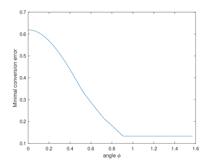
Refer to caption
Figure 4: Minimum conversion error when transforming (1/3,𝒜γ1,N1​(|0⟩​⟨0|),𝒜γ1,N1​(|1⟩​⟨1|))(1/3,\mathcal{A}^{\gamma_{1},N_{1}}(|0\rangle\!\langle 0|),\mathcal{A}^{\gamma_{1},N_{1}}(|1\rangle\!\langle 1|)) to (1/4,𝒜γ2,N2​(|0⟩​⟨0|),ei​ϕ​σ(1)​𝒜γ2,N2​(|1⟩​⟨1|)​e−i​ϕ​σ(1))(1/4,\mathcal{A}^{\gamma_{2},N_{2}}(|0\rangle\!\langle 0|),e^{i\phi\sigma^{(1)}}\mathcal{A}^{\gamma_{2},N_{2}}(|1\rangle\!\langle 1|)e^{-i\phi\sigma^{(1)}}) as a function of the angle ϕ∈[0,π/2]\phi\in[0,\pi/2], with γ1=0.5\gamma_{1}=0.5, N1=0.3N_{1}=0.3, γ2=0.25\gamma_{2}=0.25, and N2=0.1N_{2}=0.1.

As a final example, we plot the minimum conversion error in (3.30) when transforming the box

(1/3,𝒜γ1,N1​(|0⟩​⟨0|),𝒜γ1,N1​(|1⟩​⟨1|))(1/3,\mathcal{A}^{\gamma_{1},N_{1}}(|0\rangle\!\langle 0|),\mathcal{A}^{\gamma_{1},N_{1}}(|1\rangle\!\langle 1|))

to the box

(1/4,𝒜γ2,N2​(|0⟩​⟨0|),ei​ϕ​σ(1)​𝒜γ2,N2​(|1⟩​⟨1|)​e−i​ϕ​σ(1))(1/4,\mathcal{A}^{\gamma_{2},N_{2}}(|0\rangle\!\langle 0|),e^{i\phi\sigma^{(1)}}\mathcal{A}^{\gamma_{2},N_{2}}(|1\rangle\!\langle 1|)e^{-i\phi\sigma^{(1)}})

as a function of the angle ϕ∈[0,π/2]\phi\in[0,\pi/2], with γ1=0.5\gamma_{1}=0.5, N1=0.3N_{1}=0.3, γ2=0.25\gamma_{2}=0.25, and N2=0.1N_{2}=0.1. To do so, we make use of the semi-definite program from Proposition 3.16. The minimum conversion error is plotted in Figure 4 as a function of the angle ϕ\phi. Intuitively, for small values of the angle ϕ\phi, it should be more difficult to perform the conversion because the states in the first box are less distinguishable than those in the second, and so we expect the error to be higher. However, as the angle ϕ\phi increases, the states in the second box become less distinguishable and so the transformation becomes easier. The difference in the prior probabilities of the boxes is a fundamental limitation that cannot be overcome, even as ϕ\phi becomes closer to π/2\pi/2, so that the minimum conversion error plateaus for angle values greater than ≈0.9\approx 0.9.

All Matlab programs that generate the above plots (along with the semi-definite programs) are available with the arXiv ancillary files of this paper.

7 Asymptotic transformation task

Let ρX​A\rho_{XA} and σX​B\sigma_{XB} be c-q states explicitly given by

ρX​A\displaystyle\rho_{XA} =p⁡|0⟩​⟨0|⊗ρ0+(1−p)​|1⟩​⟨1|⊗ρ1,\displaystyle=p|0\rangle\!\langle 0|\otimes\rho_{0}+(1-p)|1\rangle\!\langle 1|\otimes\rho_{1}, (7.1)
σX​B\displaystyle\sigma_{XB} =q⁡|0⟩​⟨0|⊗σ0+(1−q)​|1⟩​⟨1|⊗σ1,\displaystyle=q|0\rangle\!\langle 0|\otimes\sigma_{0}+(1-q)|1\rangle\!\langle 1|\otimes\sigma_{1}, (7.2)

with ρ0,ρ1\rho_{0},\rho_{1} states of a quantum system AA, and σ0,σ1\sigma_{0},\sigma_{1} states of a quantum system BB. Moreover, we assume that p,q∈[0,1]p,q\in[0,1]. We use the short-hand notation p→≔(p,1−p)\vec{p}\coloneqq(p,1-p) and q→≔(q,1−q)\vec{q}\coloneqq(q,1-q) for the prior (distribution) of ρX​A\rho_{XA} and σX​B\sigma_{XB} respectively and write p→≻q→\vec{p}\succ\vec{q} if p→\vec{p} majorizes q→\vec{q}. Let ρX​A(n)\rho_{XA}^{(n)} and σX​B(m)\sigma_{XB}^{(m)} be as follows:

ρX​A(n)\displaystyle\rho_{XA}^{(n)} =p⁡|0⟩​⟨0|⊗ρ0⊗n+(1−p)​|1⟩​⟨1|⊗ρ1⊗n,\displaystyle=p|0\rangle\!\langle 0|\otimes\rho_{0}^{\otimes n}+(1-p)|1\rangle\!\langle 1|\otimes\rho_{1}^{\otimes n}, (7.3)
σX​B(m)\displaystyle\sigma_{XB}^{(m)} =q⁡|0⟩​⟨0|⊗σ0⊗m+(1−q)​|1⟩​⟨1|⊗σ1⊗m.\displaystyle=q|0\rangle\!\langle 0|\otimes\sigma_{0}^{\otimes m}+(1-q)|1\rangle\!\langle 1|\otimes\sigma_{1}^{\otimes m}. (7.4)
Definition 7.1

Let ρX​A,σX​B\rho_{XA},\sigma_{XB} be c-q states, and let FO{\rm FO} denote the set of free operations. For n,m∈ℕn,m\in\mathbbm{N} and ε>0\varepsilon>0, we say that there exists a (n,m,ε)(n,m,\varepsilon) FO{\rm FO}-transformation protocol for the states ρX​A\rho_{XA} and σX​B\sigma_{XB} if

dFO′​(ρX​A(n)↦σX​B(m))≤ε.\displaystyle d^{\prime}_{\operatorname{FO}}(\rho^{(n)}_{XA}\mapsto\sigma^{(m)}_{XB})\leq\varepsilon. (7.5)

That is, there exists an 𝒜∈FO\mathcal{A}\in{\rm FO} such that

D′​(𝒜⁡(ρX​A(n)),σX​B(m))≤ε.\displaystyle D^{\prime}\!\left(\mathcal{A}(\rho_{XA}^{(n)}),\sigma^{(m)}_{XB}\right)\leq\varepsilon. (7.6)

We denote such a transformation protocol in short by the notation ρX​A↦σX​B\rho_{XA}\mapsto\sigma_{XB}.

Definition 7.2

The rate R≥0R\geq 0 is an achievable rate for the transformation ρX​A↦σX​B\rho_{XA}\mapsto\sigma_{XB} under free operations FO{\rm FO}, if for all ε,δ>0\varepsilon,\delta>0 and n∈ℕn\in\mathbbm{N} large enough there exists an (n,⌊n⁡(R−δ)⌋,ε)(n,\lfloor n(R-\delta)\rfloor,\varepsilon) FO{\rm FO}-transformation protocol. The optimal rate is given by the supremum over all achievable rates, and is denoted by

RFO​(ρX​A↦σX​B)=sup{R≥0|R​ achievable rate under FO}.\displaystyle R_{\operatorname{FO}}(\rho_{XA}\mapsto\sigma_{XB})=\sup\left\{R\geq 0\Big|R\text{ achievable rate under ${\rm FO}$}\right\}. (7.7)

In particular, in the case of free operations being CPTPA{\rm{CPTP}}_{A} we write

R⁡(ρX​A↦σX​B)≡RCPTPA​(ρX​A↦σX​B),\displaystyle R(\rho_{XA}\mapsto\sigma_{XB})\equiv R_{\operatorname{CPTP}_{A}}(\rho_{XA}\mapsto\sigma_{XB}), (7.8)

and in the case of free operations being CDS{\rm{CDS}} we write

R⋆​(ρX​A↦σX​B)≡RCDS​(ρX​A↦σX​B).\displaystyle R^{\star}(\rho_{XA}\mapsto\sigma_{XB})\equiv R_{\operatorname{CDS}}(\rho_{XA}\mapsto\sigma_{XB}). (7.9)

Note that by the inclusion CPTPA⊂CDS{\rm{CPTP}}_{A}\subset{\rm{CDS}} we immediately get the inequality

R⁡(ρX​A↦σX​B)≤R⋆​(ρX​A↦σX​B).\displaystyle R(\rho_{XA}\mapsto\sigma_{XB})\leq R^{\star}(\rho_{XA}\mapsto\sigma_{XB}). (7.10)
Definition 7.3 (Strong converse rate)

The rate R≥0R\geq 0 is a strong converse rate for the transformation ρX​A↦σX​B\rho_{XA}\mapsto\sigma_{XB} under free operations FO{\rm FO}, if for all ε,δ>0\varepsilon,\delta>0 and n∈ℕn\in\mathbbm{N} large enough there does not exist an (n,⌈n⁡(R+δ)⌉,ε)(n,\lceil n(R+\delta)\rceil,\varepsilon) FO{\rm FO}-transformation protocol. The optimal strong converse rate is given by the infimum over all strong converse rates, and is denoted by

R~FO​(ρX​A↦σX​B)=inf{R≥0|R​ strong converse rate under F​O}.\displaystyle\widetilde{R}_{\operatorname{FO}}(\rho_{XA}\mapsto\sigma_{XB})=\inf\left\{R\geq 0\,\Big|\,R\text{ strong converse rate under $FO$}\right\}. (7.11)

In particular, in the case of free operations being CPTPA{\rm{CPTP}}_{A} we write

R~​(ρX​A↦σX​B)≡R~CPTPA​(ρX​A↦σX​B),\displaystyle\widetilde{R}(\rho_{XA}\mapsto\sigma_{XB})\equiv\widetilde{R}_{\operatorname{CPTP}_{A}}(\rho_{XA}\mapsto\sigma_{XB}), (7.12)

and in the case of free operations being CDS{\rm{CDS}} we write

R~⋆​(ρX​A↦σX​B)≡R~CDS​(ρX​A↦σX​B).\displaystyle\widetilde{R}^{\star}(\rho_{XA}\mapsto\sigma_{XB})\equiv\widetilde{R}_{\operatorname{CDS}}(\rho_{XA}\mapsto\sigma_{XB}). (7.13)

By definition, we have

RFO​(ρX​A↦σX​B)≤R~FO​(ρX​A↦σX​B),\displaystyle R_{\operatorname{FO}}(\rho_{XA}\mapsto\sigma_{XB})\leq\widetilde{R}_{\operatorname{FO}}(\rho_{XA}\mapsto\sigma_{XB}), (7.14)

and, moreover, by again using the fact that CPTPA⊂CDS{\rm{CPTP}}_{A}\subset{\rm{CDS}}, we get the inequality

R~​(ρX​A↦σX​B)≤R~⋆​(ρX​A↦σX​B).\displaystyle\widetilde{R}(\rho_{XA}\mapsto\sigma_{XB})\leq\widetilde{R}^{\star}(\rho_{XA}\mapsto\sigma_{XB}). (7.15)

The following theorem gives expressions for the optimal achievable and strong converse rates for the transformation ρX​A↦σX​B\rho_{XA}\mapsto\sigma_{XB} under both CDS{\rm{CDS}} and CPTPA{\rm{CPTP}}_{A}. Note that in the following we interpret ∞∞\frac{\infty}{\infty} as ∞\infty.

Theorem 7.4

Let ρX​A\rho_{XA} and σX​B\sigma_{XB} be the c-q states defined through (7.1) and (7.2) with p,q∈(0,1)p,q\in(0,1).

For free operations being CDS{\rm CDS} we have: for ξ⁡(σ0,σ1)>0\xi(\sigma_{0},\sigma_{1})>0

R⋆​(ρX​A↦σX​B)=R~⋆​(ρX​A↦σX​B)=ξ⁡(ρ0,ρ1)ξ⁡(σ0,σ1).\displaystyle R^{\star}(\rho_{XA}\mapsto\sigma_{XB})=\widetilde{R}^{\star}(\rho_{XA}\mapsto\sigma_{XB})=\frac{\xi(\rho_{0},\rho_{1})}{\xi(\sigma_{0},\sigma_{1})}. (7.16)

For ξ⁡(σ0,σ1)=0\xi(\sigma_{0},\sigma_{1})=0 and ξ⁡(ρ0,ρ1)>0\xi(\rho_{0},\rho_{1})>0 we have

R⋆​(ρX​A↦σX​B)=R~⋆​(ρX​A↦σX​B)=∞.\displaystyle R^{\star}(\rho_{XA}\mapsto\sigma_{XB})=\widetilde{R}^{\star}(\rho_{XA}\mapsto\sigma_{XB})=\infty. (7.17)

For ξ⁡(σ0,σ1)=ξ⁡(ρ0,ρ1)=0\xi(\sigma_{0},\sigma_{1})=\xi(\rho_{0},\rho_{1})=0, we have

R⋆​(ρX​A↦σX​B)\displaystyle R^{\star}(\rho_{XA}\mapsto\sigma_{XB}) =R~⋆​(ρX​A↦σX​B)=∞, if​p→≻q→,\displaystyle=\widetilde{R}^{\star}(\rho_{XA}\mapsto\sigma_{XB})=\infty,\quad\quad\quad\,\,\,\,\,{\hbox{ if}}\,\,\vec{p}\succ\vec{q},\,\, (7.18)
whereasR⋆​(ρX​A↦σX​B)\displaystyle{\hbox{whereas}}\quad\,\,R^{\star}(\rho_{XA}\mapsto\sigma_{XB}) =0​and​R~⋆​(ρX​A↦σX​B)=∞,else.\displaystyle=0\,\,\,{\hbox{and}}\,\,\,\widetilde{R}^{\star}(\rho_{XA}\mapsto\sigma_{XB})=\infty,\quad{\hbox{else.}} (7.19)

For free operations being CPTPA{\rm CPTP}_{A} we have: in the case of ρX​A\rho_{XA} and σX​B\sigma_{XB} having equal priors

R⁡(ρX​A↦σX​B)=R~​(ρX​A↦σX​B)=ξ⁡(ρ0,ρ1)ξ⁡(σ0,σ1).\displaystyle R(\rho_{XA}\mapsto\sigma_{XB})=\widetilde{R}(\rho_{XA}\mapsto\sigma_{XB})=\frac{\xi(\rho_{0},\rho_{1})}{\xi(\sigma_{0},\sigma_{1})}. (7.20)

Here, we interpreted 00\frac{0}{0} as ∞\infty.

In the case of the priors being different we get

R⁡(ρX​A↦σX​B)\displaystyle R(\rho_{XA}\mapsto\sigma_{XB}) =R~​(ρX​A↦σX​B)=0,if ​ξ​(σ0,σ1)>0,\displaystyle=\widetilde{R}(\rho_{XA}\mapsto\sigma_{XB})=0,\quad\quad\quad\text{if }\xi(\sigma_{0},\sigma_{1})>0, (7.21)
R⁡(ρX​A↦σX​B)\displaystyle R(\rho_{XA}\mapsto\sigma_{XB}) =0,R~​(ρX​A↦σX​B)=∞,if ​ξ​(σ0,σ1)=0.\displaystyle=0,\,\,\,\widetilde{R}(\rho_{XA}\mapsto\sigma_{XB})=\infty,\quad\text{if }\xi(\sigma_{0},\sigma_{1})=0. (7.22)
Remark 7.5

For simplicity we excluded in Theorem 7.4 the case of singular priors, i.e. p∈{0,1}p\in\{0,1\} or q∈{0,1}q\in\{0,1\}. For completeness we now state the corresponding results on optimal and strong converse rates in these cases:

For free operations being CDS we have

R⋆​(ρX​A↦σX​B)=R~⋆​(ρX​A↦σX​B)=∞,if ​p∈{0,1},\displaystyle R^{\star}(\rho_{XA}\mapsto\sigma_{XB})=\widetilde{R}^{\star}(\rho_{XA}\mapsto\sigma_{XB})=\infty,\quad\text{if }p\in\{0,1\}, (7.23)

and for p∈(0,1)p\in(0,1) and q∈{0,1}q\in\{0,1\} we have

R⋆​(ρX​A↦σX​B)\displaystyle R^{\star}(\rho_{XA}\mapsto\sigma_{XB}) =R~⋆​(ρX​A↦σX​B)=∞,if​ξ​(ρ0,ρ1)=∞,\displaystyle=\widetilde{R}^{\star}(\rho_{XA}\mapsto\sigma_{XB})=\infty,\quad{\hbox{if}}\,\,\xi(\rho_{0},\rho_{1})=\infty,\,\, (7.24)
whereasR⋆​(ρX​A↦σX​B)\displaystyle{\hbox{whereas}}\quad\,\,R^{\star}(\rho_{XA}\mapsto\sigma_{XB}) =R~⋆​(ρX​A↦σX​B)=0,if​ξ​(ρ0,ρ1)<∞.\displaystyle=\widetilde{R}^{\star}(\rho_{XA}\mapsto\sigma_{XB})=0,\quad\,\,\,{\hbox{if}}\,\,\xi(\rho_{0},\rho_{1})<\infty. (7.25)

For free operations being CPTPA{\rm CPTP}_{A} and q∈{0,1}q\in\{0,1\} we have

R⁡(ρX​A↦σX​B)\displaystyle R(\rho_{XA}\mapsto\sigma_{XB}) =R~​(ρX​A↦σX​B)=∞,if ​p=q,\displaystyle=\widetilde{R}(\rho_{XA}\mapsto\sigma_{XB})=\infty,\quad\text{if }p=q, (7.26)
R⁡(ρX​A↦σX​B)\displaystyle R(\rho_{XA}\mapsto\sigma_{XB}) =R~​(ρX​A↦σX​B)=0,if ​p≠q.\displaystyle=\widetilde{R}(\rho_{XA}\mapsto\sigma_{XB})=0,\quad\,\,\,\text{if }p\neq q. (7.27)

And for p∈{0,1}p\in\{0,1\} and q∈(0,1)q\in(0,1) we have similarly to (7.21) and (7.22)

R⁡(ρX​A↦σX​B)\displaystyle R(\rho_{XA}\mapsto\sigma_{XB}) =R~​(ρX​A↦σX​B)=0,if ​ξ​(σ0,σ1)>0,\displaystyle=\widetilde{R}(\rho_{XA}\mapsto\sigma_{XB})=0,\quad\quad\,\,\,\,\,\,\text{if }\xi(\sigma_{0},\sigma_{1})>0, (7.28)
R⁡(ρX​A↦σX​B)\displaystyle R(\rho_{XA}\mapsto\sigma_{XB}) =0,R~​(ρX​A↦σX​B)=∞,if ​ξ​(σ0,σ1)=0.\displaystyle=0,\,\,\,\widetilde{R}(\rho_{XA}\mapsto\sigma_{XB})=\infty,\quad\text{if }\xi(\sigma_{0},\sigma_{1})=0. (7.29)
Remark 7.6

Further to what was already stated in Remark 5.15, Theorem 7.4 expresses the fact that the resource theory of symmetric distinguishability is asymptotically reversible. Indeed, the optimal asymptotic rate at which one can convert ρX​A\rho_{XA} to σX​B\sigma_{XB} is equal to the ratio of quantum Chernoff divergences. The rate at which one can convert back is thus equal to the reciprocal of the forward rate. Since the product of these two rates is equal to one, we conclude that the RTSD is asymptotically reversible.

7.1 Proof of Theorem 7.4

7.1.1 Achievability

We start the proof of Theorem 7.4 by proving the achievability part. In particular, we show the following lemma.

Lemma 7.7

Let ρX​A\rho_{XA} and σX​B\sigma_{XB} be the c-q states defined through (7.1) and (7.2) with p,q∈(0,1)p,q\in(0,1). For ξ⁡(σ0,σ1)>0\xi(\sigma_{0},\sigma_{1})>0, we have

R⋆​(ρX​A↦σX​B)\displaystyle R^{\star}(\rho_{XA}\mapsto\sigma_{XB}) ≥ξ⁡(ρ0,ρ1)ξ⁡(σ0,σ1).\displaystyle\geq\frac{\xi(\rho_{0},\rho_{1})}{\xi(\sigma_{0},\sigma_{1})}. (7.30)

Moreover, for ξ⁡(σ0,σ1)=0\xi(\sigma_{0},\sigma_{1})=0 and ξ⁡(ρ0,ρ1)>0\xi(\rho_{0},\rho_{1})>0, we get R⋆​(ρX​A↦σX​B)=∞R^{\star}(\rho_{XA}\mapsto\sigma_{XB})=\infty and in the case ξ⁡(σ0,σ1)=ξ⁡(ρ0,ρ1)=0\xi(\sigma_{0},\sigma_{1})=\xi(\rho_{0},\rho_{1})=0 we get R⋆​(ρX​A↦σX​B)=∞R^{\star}(\rho_{XA}\mapsto\sigma_{XB})=\infty if p→≻q→\vec{p}\succ\vec{q}, and R⋆​(ρX​A↦σX​B)=0R^{\star}(\rho_{XA}\mapsto\sigma_{XB})=0 otherwise.

Moreover, in the case of ρX​A\rho_{XA} and σX​B\sigma_{XB} having the same priors we have

R⁡(ρX​A↦σX​B)\displaystyle R(\rho_{XA}\mapsto\sigma_{XB}) ≥ξ⁡(ρ0,ρ1)ξ⁡(σ0,σ1).\displaystyle\geq\frac{\xi(\rho_{0},\rho_{1})}{\xi(\sigma_{0},\sigma_{1})}. (7.31)

Here, we interpreted ∞∞\frac{\infty}{\infty} and 00\frac{0}{0} as ∞\infty. In the case of priors being different we have R⁡(ρX​A↦σX​B)=0.R(\rho_{XA}\mapsto\sigma_{XB})=0.

Proof. We prove the result for free operations being CDS{\rm{CDS}}, since for free operations being CPTPA{\rm{CPTP}}_{A} the proof follows the same lines. Let us first consider the case ξ⁡(σ0,σ1)=0\xi(\sigma_{0},\sigma_{1})=0, in which case necessarily σ0=σ1≡σ\sigma_{0}=\sigma_{1}\equiv\sigma. Moreover, first assume that ξ⁡(ρ0,ρ1)=0\xi(\rho_{0},\rho_{1})=0 (which implies that ρ0=ρ1≡ρ\rho_{0}=\rho_{1}\equiv\rho) and p→≻q→\vec{p}\succ\vec{q}. In that case, there exists a λ∈[0,1]\lambda\in[0,1] such that

λ​p+(1−λ)​(1−p)=q,\displaystyle\lambda p+(1-\lambda)(1-p)=q,

and consequently

λ⁡(1−p)+(1−λ)​p=1−q.\displaystyle\lambda(1-p)+(1-\lambda)p=1-q.

Therefore, considering for every m∈ℕm\in\mathbbm{N}

ℰ0(m)​(⋅)=λ​Tr​(⋅)​σ⊗m,ℰ1(m)​(⋅)=(1−λ)​Tr​(⋅)​σ⊗m,\displaystyle\mathcal{E}^{(m)}_{0}(\cdot)=\lambda\mathrm{Tr}(\cdot)\sigma^{\otimes m},\quad\quad\mathcal{E}^{(m)}_{1}(\cdot)=(1-\lambda)\mathrm{Tr}(\cdot)\sigma^{\otimes m},

which are quantum operations summing to a CPTP map, and the corresponding CDS map

𝒩(m)=id⊗ℰ0(m)+ℱ⊗ℰ1(m),\displaystyle\mathcal{N}^{(m)}={\rm{id}}\otimes\mathcal{E}^{(m)}_{0}+{\mathcal{F}}\otimes\mathcal{E}^{(m)}_{1}, (7.32)

we get

𝒩(m)​(ρX​A)\displaystyle\mathcal{N}^{(m)}(\rho_{XA}) =(λ​p+(1−λ)​(1−p))​|0⟩​⟨0|⊗σ⊗m+(λ⁡(1−p)+(1−λ)​p)​|1⟩​⟨1|⊗σ⊗m\displaystyle=\left(\lambda p+(1-\lambda)(1-p)\right)|0\rangle\!\langle 0|\otimes\sigma^{\otimes m}+\left(\lambda(1-p)+(1-\lambda)p\right)|1\rangle\!\langle 1|\otimes\sigma^{\otimes m}
=σX​B(m).\displaystyle=\sigma_{XB}^{(m)}.

Consequently, R⋆​(ρX​A↦σX​B)=∞R^{\star}(\rho_{XA}\mapsto\sigma_{XB})=\infty, since ρX​A\rho_{XA} can be transformed to σB​X(m)\sigma_{BX}^{(m)} without error via a CDS map for an arbitrary m∈ℕm\in{\mathbb{N}}.

Consider now the case ξ⁡(ρ0,ρ1)=ξ⁡(σ0,σ1)=0\xi(\rho_{0},\rho_{1})=\xi(\sigma_{0},\sigma_{1})=0 and p→⊁q→\vec{p}\not\succ\vec{q}. In this case, using Lemma 3.14, we see that for all n,m∈ℕn,m\in\mathbbm{N}

min⁡{p,(1−p)}\displaystyle\min\{p,(1-p)\} =perr​(ρX​A)=perr​(ρX​A(n))≤(dCDS′​(ρX​A(n)↦σX​B(m))+1)​perr​(σX​B(m))\displaystyle=p_{\operatorname{err}}(\rho_{XA})=p_{\operatorname{err}}(\rho^{(n)}_{XA})\leq\left(d^{\prime}_{\operatorname{CDS}}(\rho^{(n)}_{XA}\mapsto\sigma^{(m)}_{XB})+1\right)p_{\operatorname{err}}(\sigma^{(m)}_{XB})
=(dCDS′​(ρX​A(n)↦σX​B(m))+1)​perr​(σX​B)\displaystyle=\left(d^{\prime}_{\operatorname{CDS}}(\rho^{(n)}_{XA}\mapsto\sigma^{(m)}_{XB})+1\right)p_{\operatorname{err}}(\sigma_{XB})
=(dCDS′​(ρX​A(n)↦σX​B(m))+1)​min⁡{q,1−q},\displaystyle=\left(d^{\prime}_{\operatorname{CDS}}(\rho^{(n)}_{XA}\mapsto\sigma^{(m)}_{XB})+1\right)\min\{q,1-q\},

and since min⁡{p,(1−p)}=(c+1)​min⁡{q,(1−q)}\min\{p,(1-p)\}=(c+1)\min\{q,(1-q)\} for some c>0c>0, we get

dCDS′​(ρX​A(n)↦σX​B(m))≥c>0\displaystyle d^{\prime}_{\operatorname{CDS}}(\rho^{(n)}_{XA}\mapsto\sigma^{(m)}_{XB})\geq c>0

for all n,m∈ℕn,m\in\mathbbm{N}, and hence R⋆​(ρX​A↦σX​B)=0R^{\star}(\rho_{XA}\mapsto\sigma_{XB})=0.

Now consider the case in which ξ⁡(σ0,σ1)=0\xi(\sigma_{0},\sigma_{1})=0 but ξ⁡(ρ0,ρ1)>0\xi(\rho_{0},\rho_{1})>0. Assume without loss of generality that q≤1−qq\leq 1-q, and for all n∈ℕn\in\mathbbm{N}, let {Λ0(n),Λ1(n)}\{\Lambda^{(n)}_{0},\Lambda^{(n)}_{1}\} denote the optimal POVM for discriminating the quantum states ρ0⊗n\rho_{0}^{\otimes n} and ρ1⊗n\rho_{1}^{\otimes n} of the c-q state ρX​A(n)\rho^{(n)}_{XA}. Moreover, for all m∈ℕm\in\mathbbm{N}, let

ℰ0(n,m)(⋅)=Tr(Λ1(n)⋅)σ⊗m,ℰ1(n,m)(⋅)=Tr(Λ0(n)⋅)σ⊗m,\displaystyle\mathcal{E}^{(n,m)}_{0}(\cdot)=\mathrm{Tr}(\Lambda^{(n)}_{1}\cdot)\sigma^{\otimes m},\quad\quad\mathcal{E}^{(n,m)}_{1}(\cdot)=\mathrm{Tr}(\Lambda^{(n)}_{0}\cdot)\sigma^{\otimes m}, (7.33)

which are quantum operations summing to a CPTP map, and define the corresponding CDS map

𝒩(n,m)=id⊗ℰ0(n,m)+ℱ⊗ℰ1(n,m).\displaystyle\mathcal{N}^{(n,m)}={\rm{id}}\otimes\mathcal{E}^{(n,m)}_{0}+{\mathcal{F}}\otimes\mathcal{E}^{(n,m)}_{1}.

This gives

𝒩(n,m)​(ρX​A(n))=perr​(ρX​A(n))​|0⟩​⟨0|⊗σ⊗m+(1−perr​(ρX​A(n)))​|1⟩​⟨1|⊗σ⊗m.\displaystyle\mathcal{N}^{(n,m)}(\rho_{XA}^{(n)})=p_{\operatorname{err}}(\rho_{XA}^{(n)})|0\rangle\!\langle 0|\otimes\sigma^{\otimes m}+(1-p_{\operatorname{err}}(\rho_{XA}^{(n)}))|1\rangle\!\langle 1|\otimes\sigma^{\otimes m}.

Now choose nn large enough such that perr​(ρX​A(n))≤qp_{\operatorname{err}}(\rho_{XA}^{(n)})\leq q, which gives that the prior of 𝒩(n,m)​(ρX​A(n))\mathcal{N}^{(n,m)}(\rho_{XA}^{(n)}) majorises the prior of σX​B(m)\sigma_{XB}^{(m)}. Using the above, i.e., the construction around (7.32), we can find a CDS map transforming 𝒩(n,m)​(ρX​A(n))\mathcal{N}^{(n,m)}(\rho_{XA}^{(n)}) to σX​B(m)\sigma_{XB}^{(m)} for all mm without error. This implies that R⋆​(ρX​A↦σX​B)=∞R^{\star}(\rho_{XA}\mapsto\sigma_{XB})=\infty.

Next consider the case in which ξ⁡(σ0,σ1)>0\xi(\sigma_{0},\sigma_{1})>0. We can assume without loss of generality that ξ⁡(ρ0,ρ1)>0\xi(\rho_{0},\rho_{1})>0, since otherwise (7.31) is trivially satisfied. The case ξ⁡(ρ0,ρ1)=∞\xi(\rho_{0},\rho_{1})=\infty follows by Lemma 3.3, i.e., by the fact that we can transform any infinite-resource state to any other c-q state via CDS maps without error. Note here that ξ⁡(ρ0,ρ1)=∞\xi(\rho_{0},\rho_{1})=\infty if and only if ρ0\rho_{0} and ρ1\rho_{1} have orthogonal supports. Furthermore, the case in which ξ⁡(ρ0,ρ1)<∞\xi(\rho_{0},\rho_{1})<\infty and ξ⁡(σ0,σ1)=∞\xi(\sigma_{0},\sigma_{1})=\infty follows from the fact that any transformation from a finite resource to an infinite-resource has infinite error with respect to the scaled trace distance D′D^{\prime}.

Let us therefore now finally consider the case in which 0<ξ⁡(ρ0,ρ1),ξ⁡(σ0,σ1)<∞0<\xi(\rho_{0},\rho_{1}),\,\xi(\sigma_{0},\sigma_{1})<\infty, and fix ε,δ>0\varepsilon,\delta>0. By Theorem 4.7 we can find for all δ1>0\delta_{1}>0, an N1∈ℕN_{1}\in\mathbbm{N} such that for all n≥N1n\geq N_{1} there exists a CDS map 𝒩1\mathcal{N}_{1} such that

𝒩1​(ρX​A(n))=γX​Q(Mn),\displaystyle\mathcal{N}_{1}(\rho^{(n)}_{XA})=\gamma_{XQ}^{(M_{n})},

where γX​Q(Mn)\gamma_{XQ}^{(M_{n})} is the MnM_{n}-golden unit defined in (3.10) with

log⁡Mnn≥ξ⁡(ρ0,ρ1)−δ1.\displaystyle\frac{\log M_{n}}{n}\geq\xi(\rho_{0},\rho_{1})-\delta_{1}. (7.34)

Since ξ⁡(ρ0,ρ1)>0\xi(\rho_{0},\rho_{1})>0, without loss of generality even ξ⁡(ρ0,ρ1)>δ1\xi(\rho_{0},\rho_{1})>\delta_{1} by picking δ1\delta_{1} small enough, we also see that the sequence (Mn)n≥N(M_{n})_{n\geq N} goes to infinity for n→∞n\to\infty. For each MnM_{n} consider mn∈ℕm_{n}\in\mathbbm{N} to be the unique number such that

ξc⋆,ε​(σX​B(mn))≤log⁡Mn≤ξc⋆,ε​(σX​B(mn+1)).\displaystyle\xi^{\star,\varepsilon}_{c}(\sigma_{XB}^{(m_{n})})\leq\log M_{n}\leq\xi^{\star,\varepsilon}_{c}(\sigma_{XB}^{(m_{n}+1)}). (7.35)

First, note that we also get mn→n→∞∞m_{n}\xrightarrow[n\to\infty]{}\infty because Mn→n→∞∞M_{n}\xrightarrow[n\to\infty]{}\infty. Also note that as each ξc⋆,ε​(σX​B(mn))\xi^{\star,\varepsilon}_{c}(\sigma_{XB}^{(m_{n})}) is finite there exists a CDS map 𝒩2\mathcal{N}_{2} such that

D′​(𝒩2​(γX​Q(Mn)),σX​B(mn))≤ε\displaystyle D^{\prime}\!\left(\mathcal{N}_{2}(\gamma_{XQ}^{(M_{n})}),\sigma_{XB}^{(m_{n})}\right)\leq\varepsilon

and hence in total

D′​(𝒩2∘𝒩1​(ρX​A′(n)),σX​B(mn))≤ε.\displaystyle D^{\prime}\!\left(\mathcal{N}_{2}\circ\mathcal{N}_{1}(\rho_{XA^{\prime}}^{(n)}),\sigma_{XB}^{(m_{n})}\right)\leq\varepsilon.

Moreover, we have by (7.34) and (7.35)

ξc⋆,ε​(σX​B(mn+1))n≥log⁡Mnn≥ξ⁡(ρ0,ρ1)−δ1.\displaystyle\frac{\xi^{\star,\varepsilon}_{c}(\sigma^{(m_{n}+1)}_{XB})}{n}\geq\frac{\log M_{n}}{n}\geq\xi(\rho_{0},\rho_{1})-\delta_{1}. (7.36)

By Theorem 5.13 we can pick for all δ2>0\delta_{2}>0, an N2∈ℕN_{2}\in\mathbbm{N} such that for all n≥max⁡{N1,N2}n\geq\max\{N_{1},N_{2}\} we have

ξc⋆,ε​(σX​B(mn+1))mn+1≤ξ⁡(σ0,σ1)+δ2\frac{\xi^{\star,\varepsilon}_{c}(\sigma^{(m_{n}+1)}_{XB})}{m_{n}+1}\leq\xi(\sigma_{0},\sigma_{1})+\delta_{2}

and therefore

mn+1n​(ξ⁡(σ0,σ1)+δ2)≥log⁡Mnn≥ξ⁡(ρ0,ρ1)−δ1.\displaystyle\frac{m_{n}+1}{n}\left(\xi(\sigma_{0},\sigma_{1})+\delta_{2}\right)\geq\frac{\log M_{n}}{n}\geq\xi(\rho_{0},\rho_{1})-\delta_{1}. (7.37)

As δ1,δ2>0\delta_{1},\delta_{2}>0 are arbitrary, we can choose them small enough and moreover possibly nn even larger such that

ξ⁡(ρ0,ρ1)−δ1ξ⁡(σ0,σ1)+δ2−1n≥ξ⁡(ρ0,ρ1)ξ⁡(σ0,σ1)−δ.\displaystyle\frac{\xi(\rho_{0},\rho_{1})-\delta_{1}}{\xi(\sigma_{0},\sigma_{1})+\delta_{2}}-\frac{1}{n}\geq\frac{\xi(\rho_{0},\rho_{1})}{\xi(\sigma_{0},\sigma_{1})}-\delta.

In summary, we have proven that for all ε,δ>0\varepsilon,\delta>0 and nn large enough, there exists an (n,mn,ε)(n,m_{n},\varepsilon) CDS{\rm{CDS}}-transformation protocol with

mnn≥ξ⁡(ρ0,ρ1)ξ⁡(σ0,σ1)−δ,\displaystyle\frac{m_{n}}{n}\geq\frac{\xi(\rho_{0},\rho_{1})}{\xi(\sigma_{0},\sigma_{1})}-\delta, (7.38)

which shows that R≔ξ⁡(ρ0,ρ1)ξ⁡(σ0,σ1)R\coloneqq\frac{\xi(\rho_{0},\rho_{1})}{\xi(\sigma_{0},\sigma_{1})} is an achievable rate and hence proves (7.30).  

7.1.2 Strong converse

We now prove the strong converse part of Theorem 7.4. The proof follows a similar idea as the one for proving the strong converse in the resource theory of asymmetric distinguishability [WW19a]. There, the key insight was the pseudo continuity bound for either the sandwiched Rényi relative entropy [WW19a, Lemma 1] or Petz-Rényi relative entropy [WW19a, Lemma 3]. However, here we instead use a pseudo continuity bound for the operational quantity −log⁡(perr​(⋅))-\log(p_{\operatorname{err}}(\cdot)), involving the scaled trace distance D′D^{\prime}, and holding for two arbitrary cq-states ρX​A\rho_{XA} and σX​A\sigma_{XA}:

−log⁡(perr​(ρX​A))+log⁡(perr​(σX​A))≥−log⁡(1+D′​(ρX​A,σX​A)).\displaystyle-\log(p_{\operatorname{err}}(\rho_{XA}))+\log(p_{\operatorname{err}}(\sigma_{XA}))\geq-\log\!\left(1+D^{\prime}(\rho_{XA},\sigma_{XA})\right). (7.39)

Note that (7.39) directly follows from Lemma 3.14. With that we prove the following lemma:

Lemma 7.8

Let ρX​A\rho_{XA} and σX​B\sigma_{XB} be the c-q states defined through (7.1) and (7.2) with p,q∈(0,1)p,q\in(0,1). Then we have

R~⋆​(ρX​A↦σX​B)\displaystyle\widetilde{R}^{\star}(\rho_{XA}\mapsto\sigma_{XB}) ≤ξ⁡(ρ0,ρ1)ξ⁡(σ0,σ1),\displaystyle\leq\frac{\xi(\rho_{0},\rho_{1})}{\xi(\sigma_{0},\sigma_{1})}, (7.40)

and

R~​(ρX​A↦σX​B)\displaystyle\widetilde{R}(\rho_{XA}\mapsto\sigma_{XB}) ≤ξ⁡(ρ0,ρ1)ξ⁡(σ0,σ1).\displaystyle\leq\frac{\xi(\rho_{0},\rho_{1})}{\xi(\sigma_{0},\sigma_{1})}. (7.41)

Here, we interpreted ∞∞\frac{\infty}{\infty} and 00\frac{0}{0} as ∞\infty.

Furthermore, in the case in which ξ⁡(σ0,σ1)=0\xi(\sigma_{0},\sigma_{1})=0 we get

R~​(ρX​A↦σX​B)=R~⋆​(ρX​A↦σX​B)=∞.\displaystyle\widetilde{R}(\rho_{XA}\mapsto\sigma_{XB})=\widetilde{R}^{\star}(\rho_{XA}\mapsto\sigma_{XB})=\infty. (7.42)

Proof. As R~​(ρX​A↦σX​B)≤R~⋆​(ρX​A↦σX​B)\widetilde{R}(\rho_{XA}\mapsto\sigma_{XB})\leq\widetilde{R}^{\star}(\rho_{XA}\mapsto\sigma_{XB}) we only need to show (7.40) as (7.41) directly follows. Moreover, consider ξ⁡(σ0,σ1)>0\xi(\sigma_{0},\sigma_{1})>0 as otherwise (7.40) is trivially true. Let n,m∈ℕn,m\in\mathbbm{N} and ε>0\varepsilon>0 be such that there exists an (n,m,ε)(n,m,\varepsilon) CDS-transformation protocol. Hence, there exists a CDS map 𝒩\mathcal{N} such that

D′​(𝒩⁡(ρX​A(n)),σX​B(m))≤ε.\displaystyle D^{\prime}\!\left(\mathcal{N}(\rho_{XA}^{(n)}),\sigma_{XB}^{(m)}\right)\leq\varepsilon. (7.43)

Using first monotonicity of the minimum error probability under CDS{\rm{CDS}} maps and then (7.39) we get

−log⁡(perr​(ρX​A(n)))\displaystyle-\log\!\left(p_{\operatorname{err}}(\rho_{XA}^{(n)})\right) ≥−log⁡(perr​(𝒩⁡(ρX​A(n))))≥−log⁡(perr​(σX​B(m)))−log⁡(1+ε)\displaystyle\geq-\log\!\left(p_{\operatorname{err}}(\mathcal{N}(\rho_{XA}^{(n)}))\right)\geq-\log\!\left(p_{\operatorname{err}}(\sigma^{(m)}_{XB})\right)-\log(1+\varepsilon)
≥m​ξ​(σ0,σ1)−log⁡(1+ε),\displaystyle\geq m\xi(\sigma_{0},\sigma_{1})-\log(1+\varepsilon), (7.44)

where we have used [ACMnT+07, Theorem 1] for the last inequality. This gives

−log⁡(perr​(ρX​A(n)))ξ⁡(σ0,σ1)≥m−log⁡(1+ε)ξ⁡(σ0,σ1).\displaystyle\frac{-\log\!\left(p_{\operatorname{err}}(\rho_{XA}^{(n)})\right)}{\xi(\sigma_{0},\sigma_{1})}\geq m-\frac{\log(1+\varepsilon)}{\xi(\sigma_{0},\sigma_{1})}. (7.45)

Let now δ1>0\delta_{1}>0 and consider n∈ℕn\in\mathbbm{N} large enough such that

−log⁡(perr​(ρX​A(n)))n≤ξ⁡(ρ0,ρ1)+δ1,\displaystyle\frac{-\log\!\left(p_{\operatorname{err}}(\rho_{XA}^{(n)})\right)}{n}\leq\xi(\rho_{0},\rho_{1})+\delta_{1}, (7.46)

which is possible by the results of [NS09]. Substituting this into (7.45) we get

ξ⁡(ρ0,ρ1)ξ⁡(σ0,σ1)≥mn−log⁡(1+ε)n​ξ​(σ0,σ1)−δ1ξ⁡(σ0,σ1).\displaystyle\frac{\xi(\rho_{0},\rho_{1})}{\xi(\sigma_{0},\sigma_{1})}\geq\frac{m}{n}-\frac{\log(1+\varepsilon)}{n\xi(\sigma_{0},\sigma_{1})}-\frac{\delta_{1}}{\xi(\sigma_{0},\sigma_{1})}. (7.47)

Hence, by picking δ1>0\delta_{1}>0 small enough, we see that for all ε,δ>0\varepsilon,\delta>0 and nn large enough a possible (n,m,ε)(n,m,\varepsilon) CDS{\rm{CDS}}-transformation protocol satisfies

mn<ξ⁡(ρ0,ρ1)ξ⁡(σ0,σ1)+δ,\displaystyle\frac{m}{n}<\frac{\xi(\rho_{0},\rho_{1})}{\xi(\sigma_{0},\sigma_{1})}+\delta, (7.48)

which shows that R≔ξ⁡(ρ0,ρ1)ξ⁡(σ0,σ1)R\coloneqq\frac{\xi(\rho_{0},\rho_{1})}{\xi(\sigma_{0},\sigma_{1})} is a strong converse rate and finishes the proof.

It remains to discuss the case ξ⁡(σ0,σ1)=0\xi(\sigma_{0},\sigma_{1})=0, in which case σ0=σ1≡σ\sigma_{0}=\sigma_{1}\equiv\sigma, and to show that then R~​(ρX​A↦σX​B)=R~⋆​(ρX​A↦σX​B)=∞.\widetilde{R}(\rho_{XA}\mapsto\sigma_{XB})=\widetilde{R}^{\star}(\rho_{XA}\mapsto\sigma_{XB})=\infty. Consider for all n,m∈ℕn,m\in\mathbbm{N} the CPTP map ℰ(m)=Tr⁡(⋅)​σ⊗m\mathcal{E}^{(m)}=\mathrm{Tr}(\cdot)\sigma^{\otimes m} and note that

(id⊗ℰ(m))​(ρX​A(n))=p⁡|0⟩​⟨0|⊗σ⊗m+(1−p)​|1⟩​⟨1|⊗σ⊗m.\displaystyle\left({\rm{id}}\otimes\mathcal{E}^{(m)}\right)(\rho^{(n)}_{XA})=p|0\rangle\!\langle 0|\otimes\sigma^{\otimes m}+(1-p)|1\rangle\!\langle 1|\otimes\sigma^{\otimes m}.

Hence,

D′​((id⊗ℰ(m))​(ρX​A(n)),σX​B(m))=‖(id⊗ℰ(m))​(ρX​A(n))−σX​B(m)‖12​perr​(σX​B(m))=|p−q|min⁡{q,1−q}<∞.\displaystyle D^{\prime}\!\left(\left({\rm{id}}\otimes\mathcal{E}^{(m)}\right)(\rho^{(n)}_{XA}),\sigma^{(m)}_{XB}\right)=\frac{\left\|\left({\rm{id}}\otimes\mathcal{E}^{(m)}\right)(\rho^{(n)}_{XA})-\sigma^{(m)}_{XB}\right\|_{1}}{2p_{\operatorname{err}}(\sigma^{(m)}_{XB})}=\frac{|p-q|}{\min\{q,1-q\}}<\infty.

Therefore, for ε≔|p−q|min⁡{q,1−q}\varepsilon\coloneqq\frac{|p-q|}{\min\{q,1-q\}} fixed and all n,m∈ℕn,m\in\mathbbm{N} we have found a (n,m,ε)(n,m,\varepsilon) transformation protocol (under both CPTPA{\rm{CPTP}}_{A} and CDS{\rm{CDS}}) which implies that

R~​(ρX​A↦σX​B)=R~⋆​(ρX​A↦σX​B)=∞,\widetilde{R}(\rho_{XA}\mapsto\sigma_{XB})=\widetilde{R}^{\star}(\rho_{XA}\mapsto\sigma_{XB})=\infty, (7.49)

concluding the proof.  

8 Summary and open questions

In summary, we have introduced the resource theory of symmetric distinguishability (RTSD) and have answered many of the fundamental questions associated with it. In particular, we have developed an axiomatic approach to the RTSD, which led to the conclusion that CDS maps are the natural choice for free operations, with CPTPA maps being a special case. We then introduced the golden units of the RTSD and argued why a particular scaled trace distance is a more appropriate figure of merit for approximate transformations, instead of the standard trace distance. We finally defined and studied the tasks of dilution, distillation, and transformation, in the exact and approximate cases, both in the one-shot and asymptotic scenarios. We proved that the rate at which asymptotic transformations are possible is equal to the ratio of quantum Chernoff divergences of the elementary information sources, and we thus concluded that the RTSD is asymptotically reversible.

Going forward from here, it would be interesting to generalize the RTSD that we developed in this paper for elementary information sources to more general information sources, i.e., to c-q states for which the classical alphabet has a size greater than two. We note here that many of the concepts considered in our paper, such as the basic axioms for the RTSD, CDS maps, and the scaled trace distance D′​(⋅,⋅)D^{\prime}(\cdot,\cdot) already apply to this more general setting. In light of the seminal result in [Li16], it is a tantalizing possibility that the optimal conversion rate between quantum information sources would be equal to a ratio of multiple-state Chernoff divergences, as a generalization of Theorem 7.4, but it remains open to determine if it is the case. It is also interesting to determine expressions for the one-shot distillable-SD and SD-cost, as generalizations of ξmin\xi_{\min} and ξmax\xi_{\max}. As an additional open direction, it is worth exploring whether there is an operational interpretation of the scaled trace distance D′​(⋅,⋅)D^{\prime}(\cdot,\cdot) that we introduced in Section 3.2. Finally, it is an open question to determine if the one-shot approximate SD-cost can be evaluated by a semi-definite program. We prove in Appendix F that the two variants of approximate SD-cost (based on CPTPA and CDS maps) can be evaluated by means of bilinear programs, so that the methods of [HKT20] can be used to evaluate these quantities. However, it is not clear to us if these bilinear programs can be simplified further to semi-definite programs.

Acknowledgements—We thank Sumeet Khatri for insightful discussions and contributions at the early stage of this project. MMW acknowledges support from the National Science Foundation under Grant No. 1907615, as well as Stanford QFARM and AFOSR (FA9550-19-1-0369). GG acknowledges support from the Natural Sciences and Engineering Research Council of Canada (NSERC). RS acknowledges support from the Cambridge Commonwealth, European and International Trust.

Appendix A General properties of the axiomatic framework of the RTSD

In this appendix, we discuss a number of consequences of Axioms I-V, and the preorder of SD, introduced in Section 2. We also define general resource measures to quantify symmetric distinguishability, and we provide several examples of such measures.

Lemma A.1

The preorder of SD satisfies the following properties:

  1. 1.

    Minimal Elements. For all ρX​A∈𝔇⁡(X​A)\rho_{XA}\in\mathfrak{D}(XA) and πX′⊗ωA′∈𝔇⁡(X′​A′)\pi_{X^{\prime}}\otimes\omega_{A^{\prime}}\in\mathfrak{D}(X^{\prime}A^{\prime}) we have

    πX′⊗ωA′≺ρX​A.\pi_{X^{\prime}}\otimes\omega_{A^{\prime}}\prec\rho_{XA}\;. (A.1)
  2. 2.

    Maximal Elements. For all ρX​A∈𝔇⁡(X​A)\rho_{XA}\in\mathfrak{D}(XA), {px}x=1|X|\{p_{x}\}_{x=1}^{|X|} a probability distribution, and A′A^{\prime} a quantum system with |A′|≥|X||A^{\prime}|\geq|X|, we have

    ρX​A≺|1⟩​⟨1|X∼∑x=1|X|px​|x⟩​⟨x|X⊗|x⟩​⟨x|A′.\rho_{XA}\prec|1\rangle\!\langle 1|_{X}\sim\sum_{x=1}^{|X|}p_{x}|x\rangle\!\langle x|_{X}\otimes|x\rangle\!\langle x|_{A^{\prime}}\;. (A.2)
  3. 3.

    Reduction to Majorisation. For ρX,σX∈𝒟⁡(X)\rho_{X},\sigma_{X}\in\mathcal{D}(X) classical states of the same dimension, the preorder of SD is equivalent to the majorisation preorder.

Proof. The first property follows immediately from Axiom III and Axiom V. For the second property, first observe that Axiom III implies that |1⟩​⟨1|X∼|1⟩​⟨1|X⊗ωA|1\rangle\!\langle 1|_{X}\sim|1\rangle\!\langle 1|_{X}\otimes\omega_{A} for some ωA\omega_{A}. From the form of CDS maps we get that |1⟩​⟨1|X⊗ωA|1\rangle\!\langle 1|_{X}\otimes\omega_{A} can be converted to any cq-state in 𝔇⁡(X​A′)\mathfrak{D}(XA^{\prime}). Hence, since 𝔉⁡(X​A→X​A′)=CDS⁡(X​A→X​A′)\mathfrak{F}(XA\to XA^{\prime})={\rm CDS}(XA\to XA^{\prime}) (see Lemma 2.3) the assertion follows. For the third property, note that by Axioms I, III, and V,

ρX≺σX\displaystyle\rho_{X}\prec\sigma_{X} (A.3)

with respect to the preorder of SD if and only if

ρX=TrX′∘𝒫X​X′​(σX⊗πX′),\displaystyle\rho_{X}={\rm Tr}_{X^{\prime}}\circ\mathcal{P}_{XX^{\prime}}\left(\sigma_{X}\otimes\pi_{X^{\prime}}\right), (A.4)

for some classical system X′X^{\prime} and permutation channel 𝒫X​X′\mathcal{P}_{XX^{\prime}} on the joint classical system X​X′XX^{\prime}. The above channels are known as noisy operations [HHO03]. First, observe that noisy operations are doubly stochastic, so that if such a permutation channel 𝒫X​X′\mathcal{P}_{XX^{\prime}} exists, then σX\sigma_{X} majorizes ρX\rho_{X}.

Conversely, suppose ρ=∑y=1mty​Uy​σ​Uy\rho=\sum_{y=1}^{m}t_{y}U_{y}\sigma U_{y} where {ty}y=1m\{t_{y}\}_{y=1}^{m} are the components of a probability distribution, UyU_{y} are permutation matrices on system XX, and for convenience of the exposition here we removed the subscript XX. It is well known that such {ty}\{t_{y}\} and {Uy}\{U_{y}\} exist iff ρ≺σ\rho\prec\sigma. Suppose that ty=nynt_{y}=\frac{n_{y}}{n} are rational components where n=∑y=1mnyn=\sum_{y=1}^{m}n_{y} is the common denominator and each ny∈ℕn_{y}\in\mathbb{N}. Let X′X^{\prime} be a classical system of dimension |X′|=n|X^{\prime}|=n. Define a permutation matrix PX​X′P_{XX^{\prime}} by its action on the basis elements

PX​X′​(|x⟩X⊗|x′⟩X′)=(Uyx′​|x⟩X)⊗|x′⟩X′∀x∈[|X|],x′∈[n],P_{XX^{\prime}}\left(|x\rangle_{X}\otimes|x^{\prime}\rangle_{X^{\prime}}\right)=\left(U_{y_{x^{\prime}}}|x\rangle_{X}\right)\otimes|x^{\prime}\rangle_{X^{\prime}}\quad\quad\forall\;x\in[|X|]\;,\;x^{\prime}\in[n],

where yx′∈[m]y_{x^{\prime}}\in[m] is the index satisfying

∑z=1yx′−1nz≤x′≤∑z=1yx′nz,\sum_{z=1}^{y_{x^{\prime}}-1}n_{z}\leq x^{\prime}\leq\sum_{z=1}^{y_{x^{\prime}}}n_{z}, (A.5)

and we used the convention that the left-hand side of the above inequality is zero for yx′=1y_{x^{\prime}}=1. With this definition we have

TrX′∘𝒫X​X′​(σX⊗πX′)=1m​∑x′=1nUyx′​σX​Uyx′†=1m​∑y=1mny​Uy​σ​Uy†=∑y=1mty​Uy​σX​Uy=ρX.\displaystyle{\rm Tr}_{X^{\prime}}\circ\mathcal{P}_{XX^{\prime}}\left(\sigma_{X}\otimes\pi_{X^{\prime}}\right)=\frac{1}{m}\sum_{x^{\prime}=1}^{n}U_{y_{x^{\prime}}}\sigma_{X}U_{y_{x^{\prime}}}^{\dagger}=\frac{1}{m}\sum_{y=1}^{m}n_{y}U_{y}\sigma U_{y}^{\dagger}=\sum_{y=1}^{m}t_{y}U_{y}\sigma_{X}U_{y}=\rho_{X}\;.

Therefore, noisy operations can approximate any mixture of unitaries arbitrarily well.  

Note that the lemma above indicates that |1⟩​⟨1|X|1\rangle\!\langle 1|_{X} is the maximal resource in the fixed dimension of XX. If, for example, X′X^{\prime} is another system with a higher dimension |X′|>|X||X^{\prime}|>|X| then

|1⟩​⟨1|X≺|1⟩​⟨1|X′.|1\rangle\!\langle 1|_{X}\prec|1\rangle\!\langle 1|_{X^{\prime}}\;. (A.6)

That is, the ‘embedding’ of XX into X′X^{\prime} by adding zero components to matrices/vectors is not allowed in this resource theory since it can increase the value of the resource. To get the intuition behind it, consider Xiao possessing either one of the two classical states |1⟩​⟨1|X​X~|1\rangle\!\langle 1|_{X\tilde{X}} or |1⟩​⟨1|X⊗πX~|1\rangle\!\langle 1|_{X}\otimes\pi_{\tilde{X}}. In the first case, Xiao has complete information of the state in her possession since she knows the values of both the random variables X{X} and X~\tilde{X}. On the other hand, in the second case Xiao has no information about X~\tilde{X}, since it is in a uniform state. Therefore, the first state is more distinguishable than the second one and we get

|1⟩​⟨1|X∼|1⟩​⟨1|X⊗πX~≺|1⟩​⟨1|X​X~.|1\rangle\!\langle 1|_{X}\sim|1\rangle\!\langle 1|_{X}\otimes\pi_{\tilde{X}}\prec|1\rangle\!\langle 1|_{X\tilde{X}}. (A.7)

Hence, for the case X′=X​X~X^{\prime}=X\tilde{X}, (A.7) reduces (A.6). More generally, the SD of a cq-state ρX​A\rho_{XA} represents the ability of Alice to distinguish the elements in Xiao’s system. Therefore, the greater |X||X| is, the more elements there are to distinguish, and consequently, the maximal resource has greater SD. This, in particular, applies to the minimum error probability perr​(ρX​A)p_{\operatorname{err}}(\rho_{XA}). That is, suppose for example that two states ρX​A,σX′​A′∈𝔇c​q\rho_{XA},\sigma_{X^{\prime}A^{\prime}}\in\mathfrak{D}_{cq}, with |X|<|X′||X|<|X^{\prime}| satisfy

perr​(ρX​A)=perr​(σX′​A′).p_{\operatorname{err}}(\rho_{XA})=p_{\operatorname{err}}(\sigma_{X^{\prime}A^{\prime}})\;. (A.8)

Then, we can expect that σX′​A′\sigma_{X^{\prime}A^{\prime}} has more SD since Alice is able to distinguish among |X′|>|X||X^{\prime}|>|X| elements with the same error as she would have if she held ρX​A\rho_{XA}. This means in particular that if we consider inter-conversions among c-q states with different classical dimensions then the minimum error probability is not a good measure of SD. In the following subsection we show how the minimum error probability needs to be re-scaled with the classical dimension so that it becomes a proper measure of SD.

A.1 Quantification of SD

SD is quantified with functions that preserve the preorder of SD.

Definition A.2

A function f:𝔇c​q→ℝf:\mathfrak{D}_{cq}\to\mathbb{R} is called a measure of SD if:

  1. 1.

    For any ρX​A,σX′​A′∈𝔇c​q\rho_{XA},\sigma_{X^{\prime}A^{\prime}}\in\mathfrak{D}_{cq} we have

    ρX​A≺σX′​A′⇒f⁡(ρX​A)≤f⁡(σX′​A′).\rho_{XA}\prec\sigma_{X^{\prime}A^{\prime}}\quad\Rightarrow\quad f\left(\rho_{XA}\right)\leq f\left(\sigma_{X^{\prime}A^{\prime}}\right)\;. (A.9)
  2. 2.

    For the trivial state 11 (i.e. |X|=|A|=1|X|=|A|=1) we have

    f⁡(1)=0.f(1)=0\;. (A.10)

Note that from Axiom III and the second condition above, all measures of SD vanish on free states. Combining this with the property in (A.1) we conclude that measures of SD are non-negative.

Example A.3

Let

𝔻:⋃A𝒟(A)×𝒟(A)→ℝ:(ρ,σ)↦𝔻(ρ∥σ)\mathbb{D}\;:\;\bigcup_{A}\mathcal{D}(A)\times\mathcal{D}(A)\to\mathbb{R}\;:\;(\rho,\sigma)\mapsto\mathbb{D}(\rho\|\sigma)

be a relative entropy; i.e. it satisfies the DPI, additivity (under tensor products), and the normalization 𝔻(1∥1)=0\mathbb{D}(1\|1)=0. Then, the function

minω∈𝒟⁡(A)𝔻(ρX​A∥πX⊗ωA)≔log|X|−ℍ(X|A)ρ\min_{\omega\in\mathcal{D}(A)}\mathbb{D}\left(\rho_{XA}\|\pi_{X}\otimes\omega_{A}\right)\coloneqq\log|X|-\mathbb{H}(X|A)_{\rho} (A.11)

is a measure of SD, since in any quantum resource theory, a function of the form minω∈𝔉⁡(A)𝔻(ρA∥ωA)\min_{\omega\in\mathfrak{F}(A)}\mathbb{D}(\rho_{A}\|\omega_{A}) is a measure of a resource [CG19].

Example A.4 (Normalized guessing probability)

A special example of the above family of measures of SD is obtained when setting 𝔻\mathbb{D} to be the max-relative entropy DmaxD_{\max}. Specifically, in [KRS09] it was shown that the guessing probability can be written as

pguess(X|A)ρ=2minω∈𝒟⁡(A)Dmax(ρX​A∥IX⊗ωA).\displaystyle p_{\rm{guess}}(X|A)_{\rho}=2^{\min_{\omega\in\mathcal{D}(A)}D_{\max}(\rho_{XA}\|I_{X}\otimes\omega_{A})}\;.

Therefore, replacing IXI_{X} with the maximally mixed state πX\pi_{X} we get that the function

log(|X|pguess(X|A)ρ)=minω∈𝒟⁡(A)Dmax(ρX​A∥πX⊗ωA)\log\left(|X|p_{\rm{guess}}(X|A)_{\rho}\right)=\min_{\omega\in\mathcal{D}(A)}D_{\max}(\rho_{XA}\|\pi_{X}\otimes\omega_{A}) (A.12)

is a measure of SD. Note that the dimension of the classical system is included on the left-side so that the expression remains invariant under replacement of ρX​A\rho_{XA} with ρX​A⊗πX′\rho_{XA}\otimes\pi_{X^{\prime}}.

In this paper we have focused on the RTSD for the particular case in which the dimension of the classical system XX is fixed to |X|=2|X|=2. In this case, as mentioned in the main text, it suffices to consider measures of SD that behave monotonically under CDS but not necessarily under conditional noisy operations (i.e., under free operations that change the dimension of XX). The measure of SD that we have chosen in the paper is given by Definition 2.5. As shown in Theorem 4.5 it has the particularly pleasing feature of having an operational meaning in the context of SD distillation.

Appendix B Proof of Eq. (3.16) — Minimum trace distance to infinite-resource states under free operations

Let (p​ρ0,(1−p)​ρ1)\left(p\rho^{0},\left(1-p\right)\rho^{1}\right) be a pair of subnormalized states, with p∈(0,1)p\in(0,1), and ρ0\rho^{0} and ρ1\rho^{1} states. Then this pair is in one-to-one correspondence with the following classical–quantum state:

ρX​B≔p⁡|0⟩​⟨0|X⊗ρB0+(1−p)|1⟩​⟨1|X⊗ρB1.\rho_{XB}\coloneqq p|0\rangle\!\langle 0|_{X}\otimes\rho_{B}^{0}+\left(1-p\right)|1\rangle\!\langle 1|_{X}\otimes\rho_{B}^{1}. (B.1)

Let (q​σ0,(1−q)​σ1)(q\sigma^{0},\left(1-q\right)\sigma^{1}) be another pair of subnormalized states, with q∈(0,1)q\in(0,1), and σ0\sigma^{0} and σ1\sigma^{1} states. Then this pair is in one-to-one correspondence with the following classical–quantum state:

σX​B′≔q⁡|0⟩​⟨0|X⊗σB′0+(1−q)|1⟩​⟨1|X⊗σB′1.\sigma_{XB^{\prime}}\coloneqq q|0\rangle\!\langle 0|_{X}\otimes\sigma_{B^{\prime}}^{0}+\left(1-q\right)|1\rangle\!\langle 1|_{X}\otimes\sigma_{B^{\prime}}^{1}. (B.2)

The trace-distance conversion error of ρX​B\rho_{XB} to σX​B′\sigma_{XB^{\prime}} is defined as follows:

min𝒩X​B→X​B′∈CDS⁡12​‖𝒩X​B→X​B′​(ρX​B)−σX​B′‖1,\min_{\mathcal{N}_{XB\rightarrow XB^{\prime}}\in\text{$\operatorname{CDS}$}}\frac{1}{2}\left\|\mathcal{N}_{XB\rightarrow XB^{\prime}}(\rho_{XB})-\sigma_{XB^{\prime}}\right\|_{1}, (B.3)

where CDS is the set of conditional doubly stochastic (CDS) maps.

We first show that the trace-distance conversion error can be computed by means of a semi-definite program.

Proposition B.1

The trace-distance conversion error

min𝒩X​B→X​B′∈CDS⁡12​‖𝒩X​B→X′​B′​(ρX​B)−σX​B′‖1\min_{\mathcal{N}_{XB\rightarrow XB^{\prime}}\in\operatorname{CDS}}\frac{1}{2}\left\|\mathcal{N}_{XB\rightarrow X^{\prime}B^{\prime}}(\rho_{XB})-\sigma_{XB^{\prime}}\right\|_{1} (B.4)

between the initial pair (p​ρB0,(1−p)​ρB1)(p\rho_{B}^{0},\left(1-p\right)\rho_{B}^{1}) and the target pair (q​σB′0,(1−q)​σB′1)(q\sigma_{B^{\prime}}^{0},\left(1-q\right)\sigma_{B^{\prime}}^{1}) can be calculated by means of the following semi-definite program:

minYB′0,YB′1,ΓB​B′𝒩0,ΓB​B′𝒩1≥0⁡Tr⁡[YB′0+YB′1]\min_{Y_{B^{\prime}}^{0},Y_{B^{\prime}}^{1},\Gamma_{BB^{\prime}}^{\mathcal{N}^{0}},\Gamma_{BB^{\prime}}^{\mathcal{N}^{1}}\geq 0}\operatorname{Tr}[Y_{B^{\prime}}^{0}+Y_{B^{\prime}}^{1}] (B.5)

subject to

TrB′⁡[ΓB​B′𝒩0+ΓB​B′𝒩1]=IB,\operatorname{Tr}_{B^{\prime}}[\Gamma_{BB^{\prime}}^{\mathcal{N}^{0}}+\Gamma_{BB^{\prime}}^{\mathcal{N}^{1}}]=I_{B}, (B.6)
YB′0\displaystyle Y_{B^{\prime}}^{0} ≥TrB⁡[(p​ρB0)T​ΓB​B′𝒩0+((1−p)​ρB1)T​ΓB​B′𝒩1]−q​σB′0,\displaystyle\geq\operatorname{Tr}_{B}[(p\rho_{B}^{0})^{T}\Gamma_{BB^{\prime}}^{\mathcal{N}^{0}}+(\left(1-p\right)\rho_{B}^{1})^{T}\Gamma_{BB^{\prime}}^{\mathcal{N}^{1}}]-q\sigma_{B^{\prime}}^{0}, (B.7)
YB′1\displaystyle Y_{B^{\prime}}^{1} ≥TrB⁡[(p​ρB0)T​ΓB​B′𝒩1+((1−p)​ρB1)T​ΓB​B′𝒩0]−(1−q)​σB′1.\displaystyle\geq\operatorname{Tr}_{B}[(p\rho_{B}^{0})^{T}\Gamma_{BB^{\prime}}^{\mathcal{N}^{1}}+(\left(1-p\right)\rho_{B}^{1})^{T}\Gamma_{BB^{\prime}}^{\mathcal{N}^{0}}]-\left(1-q\right)\sigma_{B^{\prime}}^{1}. (B.8)

The dual program is given by

maxYB∈Herm,WB′,ZB′≥0⁡Tr⁡[YB]−q​Tr⁡[WB′​σB′0]−(1−q)​Tr⁡[ZB′​σB′1],\max_{Y_{B}\in\operatorname{Herm},W_{B^{\prime}},Z_{B^{\prime}}\geq 0}\operatorname{Tr}[Y_{B}]-q\operatorname{Tr}[W_{B^{\prime}}\sigma_{B^{\prime}}^{0}]-\left(1-q\right)\operatorname{Tr}[Z_{B^{\prime}}\sigma_{B^{\prime}}^{1}], (B.9)

subject to

WB′,ZB′\displaystyle W_{B^{\prime}},Z_{B^{\prime}} ≤IB′,\displaystyle\leq I_{B^{\prime}}, (B.10)
YB⊗IB′\displaystyle Y_{B}\otimes I_{B^{\prime}} ≤p​ρB0⊗WB′+(1−p)​ρB1⊗ZB′,\displaystyle\leq p\rho_{B}^{0}\otimes W_{B^{\prime}}+\left(1-p\right)\rho_{B}^{1}\otimes Z_{B^{\prime}}, (B.11)
YB⊗IB′\displaystyle Y_{B}\otimes I_{B^{\prime}} ≤(1−p)​ρB1⊗WB′+p​ρB0⊗ZB′.\displaystyle\leq\left(1-p\right)\rho_{B}^{1}\otimes W_{B^{\prime}}+p\rho_{B}^{0}\otimes Z_{B^{\prime}}. (B.12)

Proof. Recall that an arbitrary CDS channel has the following form:

idX⊗𝒩B→B′0+𝒫X⊗𝒩B→B′1,\operatorname{id}_{X}\otimes\mathcal{N}_{B\rightarrow B^{\prime}}^{0}+\mathcal{P}_{X}\otimes\mathcal{N}_{B\rightarrow B^{\prime}}^{1}, (B.13)

where 𝒩B→B′0\mathcal{N}_{B\rightarrow B^{\prime}}^{0} and 𝒩B→B′1\mathcal{N}_{B\rightarrow B^{\prime}}^{1} are completely positive maps such that 𝒩B→B′0+𝒩B→B′1\mathcal{N}_{B\rightarrow B^{\prime}}^{0}+\mathcal{N}_{B\rightarrow B^{\prime}}^{1} is trace preserving, and 𝒫X\mathcal{P}_{X} is a unitary channel that flips |0⟩​⟨0||0\rangle\!\langle 0| and |1⟩​⟨1||1\rangle\!\langle 1|. This means that its action on an input

p⁡|0⟩​⟨0|X⊗ρB0+(1−p)|1⟩​⟨1|X⊗ρB1p|0\rangle\!\langle 0|_{X}\otimes\rho_{B}^{0}+\left(1-p\right)|1\rangle\!\langle 1|_{X}\otimes\rho_{B}^{1} (B.14)

is as follows:

(idX⊗𝒩B→B′0+𝒫X⊗𝒩B→B′1)​(p⁡|0⟩​⟨0|X⊗ρB0+(1−p)|1⟩​⟨1|X⊗ρB1)\displaystyle\left(\operatorname{id}_{X}\otimes\mathcal{N}_{B\rightarrow B^{\prime}}^{0}+\mathcal{P}_{X}\otimes\mathcal{N}_{B\rightarrow B^{\prime}}^{1}\right)\left(p|0\rangle\!\langle 0|_{X}\otimes\rho_{B}^{0}+\left(1-p\right)|1\rangle\!\langle 1|_{X}\otimes\rho_{B}^{1}\right)
=(idX⊗𝒩B→B′0)​(p⁡|0⟩​⟨0|X⊗ρB0+(1−p)|1⟩​⟨1|X⊗ρB1)\displaystyle=\left(\operatorname{id}_{X}\otimes\mathcal{N}_{B\rightarrow B^{\prime}}^{0}\right)\left(p|0\rangle\!\langle 0|_{X}\otimes\rho_{B}^{0}+\left(1-p\right)|1\rangle\!\langle 1|_{X}\otimes\rho_{B}^{1}\right)
+(𝒫X⊗𝒩B→B′1)​(p⁡|0⟩​⟨0|X⊗ρB0+(1−p)|1⟩​⟨1|X⊗ρB1)\displaystyle\qquad+\left(\mathcal{P}_{X}\otimes\mathcal{N}_{B\rightarrow B^{\prime}}^{1}\right)\left(p|0\rangle\!\langle 0|_{X}\otimes\rho_{B}^{0}+\left(1-p\right)|1\rangle\!\langle 1|_{X}\otimes\rho_{B}^{1}\right) (B.15)
=p⁡|0⟩​⟨0|X⊗𝒩B→B′0​(ρB0)+(1−p)|1⟩​⟨1|X⊗𝒩B→B′0​(ρB1)\displaystyle=p|0\rangle\!\langle 0|_{X}\otimes\mathcal{N}_{B\rightarrow B^{\prime}}^{0}(\rho_{B}^{0})+\left(1-p\right)|1\rangle\!\langle 1|_{X}\otimes\mathcal{N}_{B\rightarrow B^{\prime}}^{0}(\rho_{B}^{1})
+p𝒫X(|0⟩⟨0|X)⊗𝒩B→B′1(ρB0)\displaystyle\qquad+p\mathcal{P}_{X}(|0\rangle\!\langle 0|_{X})\otimes\mathcal{N}_{B\rightarrow B^{\prime}}^{1}(\rho_{B}^{0})
+(1−p)𝒫X(|1⟩⟨1|X)⊗𝒩B→B′1(ρB1)\displaystyle\qquad+\left(1-p\right)\mathcal{P}_{X}(|1\rangle\!\langle 1|_{X})\otimes\mathcal{N}_{B\rightarrow B^{\prime}}^{1}(\rho_{B}^{1}) (B.16)
=p⁡|0⟩​⟨0|X⊗𝒩B→B′0​(ρB0)+(1−p)|1⟩​⟨1|X⊗𝒩B→B′0​(ρB1)\displaystyle=p|0\rangle\!\langle 0|_{X}\otimes\mathcal{N}_{B\rightarrow B^{\prime}}^{0}(\rho_{B}^{0})+\left(1-p\right)|1\rangle\!\langle 1|_{X}\otimes\mathcal{N}_{B\rightarrow B^{\prime}}^{0}(\rho_{B}^{1})
+p|1⟩⟨1|X⊗𝒩B→B′1(ρB0)+(1−p)|0⟩⟨0|X⊗𝒩B→B′1(ρB1)\displaystyle\qquad+p|1\rangle\!\langle 1|_{X}\otimes\mathcal{N}_{B\rightarrow B^{\prime}}^{1}(\rho_{B}^{0})+\left(1-p\right)|0\rangle\!\langle 0|_{X}\otimes\mathcal{N}_{B\rightarrow B^{\prime}}^{1}(\rho_{B}^{1}) (B.17)
=|0⟩​⟨0|X⊗[𝒩B→B′0​(p​ρB0)+𝒩B→B′1​((1−p)​ρB1)]\displaystyle=|0\rangle\!\langle 0|_{X}\otimes\left[\mathcal{N}_{B\rightarrow B^{\prime}}^{0}(p\rho_{B}^{0})+\mathcal{N}_{B\rightarrow B^{\prime}}^{1}(\left(1-p\right)\rho_{B}^{1})\right]
+|1⟩⟨1|X⊗[𝒩B→B′1(pρB0)+𝒩B→B′0((1−p)ρB1)].\displaystyle\qquad+|1\rangle\!\langle 1|_{X}\otimes\left[\mathcal{N}_{B\rightarrow B^{\prime}}^{1}(p\rho_{B}^{0})+\mathcal{N}_{B\rightarrow B^{\prime}}^{0}(\left(1-p\right)\rho_{B}^{1})\right]. (B.18)

The semi-definite specifications for the completely positive maps 𝒩B→B′0\mathcal{N}_{B\rightarrow B^{\prime}}^{0} and 𝒩B→B′1\mathcal{N}_{B\rightarrow B^{\prime}}^{1} are as follows:

ΓB​B′𝒩0,ΓB​B′𝒩1\displaystyle\Gamma_{BB^{\prime}}^{\mathcal{N}^{0}},\Gamma_{BB^{\prime}}^{\mathcal{N}^{1}} ≥0,\displaystyle\geq 0, (B.19)
TrB′⁡[ΓB​B′𝒩0+ΓB​B′𝒩1]\displaystyle\operatorname{Tr}_{B^{\prime}}[\Gamma_{BB^{\prime}}^{\mathcal{N}^{0}}+\Gamma_{BB^{\prime}}^{\mathcal{N}^{1}}] =IB.\displaystyle=I_{B}. (B.20)

Furthermore, the output state is given by

|0⟩​⟨0|X⊗[TrB⁡[(p​ρB0)T​ΓB​B′𝒩0]+TrB⁡[((1−p)​ρB1)T​ΓB​B′𝒩1]]+|1⟩⟨1|X⊗[TrB[(pρB0)TΓB​B′𝒩1]+TrB[((1−p)ρB1)TΓB​B′𝒩0]].|0\rangle\!\langle 0|_{X}\otimes\left[\operatorname{Tr}_{B}[(p\rho_{B}^{0})^{T}\Gamma_{BB^{\prime}}^{\mathcal{N}^{0}}]+\operatorname{Tr}_{B}[(\left(1-p\right)\rho_{B}^{1})^{T}\Gamma_{BB^{\prime}}^{\mathcal{N}^{1}}]\right]\\ +|1\rangle\!\langle 1|_{X}\otimes\left[\operatorname{Tr}_{B}[(p\rho_{B}^{0})^{T}\Gamma_{BB^{\prime}}^{\mathcal{N}^{1}}]+\operatorname{Tr}_{B}[(\left(1-p\right)\rho_{B}^{1})^{T}\Gamma_{BB^{\prime}}^{\mathcal{N}^{0}}]\right]. (B.21)

Recall that the dual semi-definite program for computing the normalized trace distance of two quantum states ρ\rho and σ\sigma is as follows (see, e.g., [WW19a]):

12​‖ρ−σ‖1=minY≥0⁡{Tr⁡[Y]:Y≥ρ−σ}.\frac{1}{2}\left\|\rho-\sigma\right\|_{1}=\min_{Y\geq 0}\left\{\operatorname{Tr}[Y]:Y\geq\rho-\sigma\right\}. (B.22)

So in this case, it follows that

min𝒩X​B→X​B′∈CDS⁡12​‖𝒩X​B→X​B′​(ρX​B)−σX​B′‖1=minYX​B′≥0⁡{Tr⁡[YX​B′]:YX​B′≥𝒩X​B→X​B′​(ρX​B)−σX​B′},\min_{\mathcal{N}_{XB\rightarrow XB^{\prime}}\in\text{$\operatorname{CDS}$}}\frac{1}{2}\left\|\mathcal{N}_{XB\rightarrow XB^{\prime}}(\rho_{XB})-\sigma_{XB^{\prime}}\right\|_{1}\\ =\min_{Y_{XB^{\prime}}\geq 0}\left\{\operatorname{Tr}[Y_{XB^{\prime}}]:Y_{XB^{\prime}}\geq\mathcal{N}_{XB\rightarrow XB^{\prime}}(\rho_{XB})-\sigma_{XB^{\prime}}\right\}, (B.23)

where we have now called the output system XX for clarity. Then the SDP for the trace-distance conversion error is given by

minYX​B′≥0⁡Tr⁡[YX​B′]\min_{Y_{XB^{\prime}}\geq 0}\operatorname{Tr}[Y_{XB^{\prime}}] (B.24)

subject to

ΓB​B′𝒩0,ΓB​B′𝒩1\displaystyle\Gamma_{BB^{\prime}}^{\mathcal{N}^{0}},\Gamma_{BB^{\prime}}^{\mathcal{N}^{1}} ≥0,\displaystyle\geq 0, (B.25)
TrB′⁡[ΓB​B′𝒩0+ΓB​B′𝒩1]\displaystyle\operatorname{Tr}_{B^{\prime}}[\Gamma_{BB^{\prime}}^{\mathcal{N}^{0}}+\Gamma_{BB^{\prime}}^{\mathcal{N}^{1}}] =IB,\displaystyle=I_{B}, (B.26)
YX​B′≥|0⟩​⟨0|X⊗[TrB⁡[(p​ρB0)T​ΓB​B′𝒩0]+TrB⁡[((1−p)​ρB1)T​ΓB​B′𝒩1]−q​σB′0]+|1⟩⟨1|X⊗[TrB[(pρB0)TΓB​B′𝒩1]+TrB[((1−p)ρB1)TΓB​B′𝒩0]−(1−q)σB′1].Y_{XB^{\prime}}\geq|0\rangle\!\langle 0|_{X}\otimes\left[\operatorname{Tr}_{B}[(p\rho_{B}^{0})^{T}\Gamma_{BB^{\prime}}^{\mathcal{N}^{0}}]+\operatorname{Tr}_{B}[(\left(1-p\right)\rho_{B}^{1})^{T}\Gamma_{BB^{\prime}}^{\mathcal{N}^{1}}]-q\sigma_{B^{\prime}}^{0}\right]\\ +|1\rangle\!\langle 1|_{X}\otimes\left[\operatorname{Tr}_{B}[(p\rho_{B}^{0})^{T}\Gamma_{BB^{\prime}}^{\mathcal{N}^{1}}]+\operatorname{Tr}_{B}[(\left(1-p\right)\rho_{B}^{1})^{T}\Gamma_{BB^{\prime}}^{\mathcal{N}^{0}}]-\left(1-q\right)\sigma_{B^{\prime}}^{1}\right]. (B.27)

It is clear that the optimal YX​B′Y_{XB^{\prime}} respects the classical–quantum structure. So this means that the final SDP can be written as follows:

minYB′0,YB′1,ΓB​B′𝒩0,ΓB​B′𝒩1≥0⁡Tr⁡[YB′0+YB′1]\min_{Y_{B^{\prime}}^{0},Y_{B^{\prime}}^{1},\Gamma_{BB^{\prime}}^{\mathcal{N}^{0}},\Gamma_{BB^{\prime}}^{\mathcal{N}^{1}}\geq 0}\operatorname{Tr}[Y_{B^{\prime}}^{0}+Y_{B^{\prime}}^{1}] (B.28)

subject to

TrB′⁡[ΓB​B′𝒩0+ΓB​B′𝒩1]=IB,\operatorname{Tr}_{B^{\prime}}[\Gamma_{BB^{\prime}}^{\mathcal{N}^{0}}+\Gamma_{BB^{\prime}}^{\mathcal{N}^{1}}]=I_{B}, (B.29)
YB′0\displaystyle Y_{B^{\prime}}^{0} ≥TrB⁡[(p​ρB0)T​ΓB​B′𝒩0]+TrB⁡[((1−p)​ρB1)T​ΓB​B′𝒩1]−q​σB′0,\displaystyle\geq\operatorname{Tr}_{B}[(p\rho_{B}^{0})^{T}\Gamma_{BB^{\prime}}^{\mathcal{N}^{0}}]+\operatorname{Tr}_{B}[(\left(1-p\right)\rho_{B}^{1})^{T}\Gamma_{BB^{\prime}}^{\mathcal{N}^{1}}]-q\sigma_{B^{\prime}}^{0}, (B.30)
YB′1\displaystyle Y_{B^{\prime}}^{1} ≥TrB⁡[(p​ρB0)T​ΓB​B′𝒩1]+TrB⁡[((1−p)​ρB1)T​ΓB​B′𝒩0]−(1−q)​σB′1.\displaystyle\geq\operatorname{Tr}_{B}[(p\rho_{B}^{0})^{T}\Gamma_{BB^{\prime}}^{\mathcal{N}^{1}}]+\operatorname{Tr}_{B}[(\left(1-p\right)\rho_{B}^{1})^{T}\Gamma_{BB^{\prime}}^{\mathcal{N}^{0}}]-\left(1-q\right)\sigma_{B^{\prime}}^{1}. (B.31)

Now we compute the dual of the semi-definite program above. Recall the standard form of primal and dual SDPs:

maxX≥0⁡{Tr⁡[A​X]:Φ⁡(X)≤B},\displaystyle\max_{X\geq 0}\left\{\operatorname{Tr}[AX]:\Phi(X)\leq B\right\}, (B.32)
minY≥0⁡{Tr⁡[B​Y]:Φ†​(Y)≥A}.\displaystyle\min_{Y\geq 0}\left\{\operatorname{Tr}[BY]:\Phi^{{\dagger}}(Y)\geq A\right\}. (B.33)

From inspecting the above, we see that

Y\displaystyle Y =[YB′00000YB′10000ΓB​B′𝒩00000ΓB​B′𝒩1],B=[I0000I0000000000],\displaystyle=\begin{bmatrix}Y_{B^{\prime}}^{0}&0&0&0\\ 0&Y_{B^{\prime}}^{1}&0&0\\ 0&0&\Gamma_{BB^{\prime}}^{\mathcal{N}^{0}}&0\\ 0&0&0&\Gamma_{BB^{\prime}}^{\mathcal{N}^{1}}\end{bmatrix},\qquad B=\begin{bmatrix}I&0&0&0\\ 0&I&0&0\\ 0&0&0&0\\ 0&0&0&0\end{bmatrix}, (B.34)
Φ†​(Y)\displaystyle\Phi^{{\dagger}}(Y) =[TrB′⁡[ΓB​B′𝒩0+ΓB​B′𝒩1]0000−TrB′⁡[ΓB​B′𝒩0+ΓB​B′𝒩1]0000YB′0−ZB′00000YB′1−ZB′1],\displaystyle=\begin{bmatrix}\operatorname{Tr}_{B^{\prime}}[\Gamma_{BB^{\prime}}^{\mathcal{N}^{0}}+\Gamma_{BB^{\prime}}^{\mathcal{N}^{1}}]&0&0&0\\ 0&-\operatorname{Tr}_{B^{\prime}}[\Gamma_{BB^{\prime}}^{\mathcal{N}^{0}}+\Gamma_{BB^{\prime}}^{\mathcal{N}^{1}}]&0&0\\ 0&0&Y_{B^{\prime}}^{0}-Z_{B^{\prime}}^{0}&0\\ 0&0&0&Y_{B^{\prime}}^{1}-Z_{B^{\prime}}^{1}\end{bmatrix}, (B.35)
A\displaystyle A =[IB0000−IB0000−q​σB′00000−(1−q)​σB′1].\displaystyle=\begin{bmatrix}I_{B}&0&0&0\\ 0&-I_{B}&0&0\\ 0&0&-q\sigma_{B^{\prime}}^{0}&0\\ 0&0&0&-\left(1-q\right)\sigma_{B^{\prime}}^{1}\end{bmatrix}. (B.36)

where

ZB′0\displaystyle Z_{B^{\prime}}^{0} ≔TrB⁡[(p​ρB0)T​ΓB​B′𝒩0+((1−p)​ρB1)T​ΓB​B′𝒩1],\displaystyle\coloneqq\operatorname{Tr}_{B}[(p\rho_{B}^{0})^{T}\Gamma_{BB^{\prime}}^{\mathcal{N}^{0}}+(\left(1-p\right)\rho_{B}^{1})^{T}\Gamma_{BB^{\prime}}^{\mathcal{N}^{1}}], (B.37)
ZB′1\displaystyle Z_{B^{\prime}}^{1} ≔TrB⁡[(p​ρB0)T​ΓB​B′𝒩1+((1−p)​ρB1)T​ΓB​B′𝒩0].\displaystyle\coloneqq\operatorname{Tr}_{B}[(p\rho_{B}^{0})^{T}\Gamma_{BB^{\prime}}^{\mathcal{N}^{1}}+(\left(1-p\right)\rho_{B}^{1})^{T}\Gamma_{BB^{\prime}}^{\mathcal{N}^{0}}]. (B.38)

Now we need to find the adjoint map of Φ†\Phi^{{\dagger}}. Consider that

Tr⁡[Φ†​(Y)​X]\displaystyle\operatorname{Tr}[\Phi^{{\dagger}}(Y)X]
=Tr⁡[TrB′⁡[ΓB​B′𝒩0+ΓB​B′𝒩1]​(XB1−XB2)]\displaystyle=\operatorname{Tr}[\operatorname{Tr}_{B^{\prime}}[\Gamma_{BB^{\prime}}^{\mathcal{N}^{0}}+\Gamma_{BB^{\prime}}^{\mathcal{N}^{1}}](X_{B}^{1}-X_{B}^{2})]
+Tr⁡[(YB′0−TrB⁡[(p​ρB0)T​ΓB​B′𝒩0+((1−p)​ρB1)T​ΓB​B′𝒩1])​XB′3]\displaystyle\qquad+\operatorname{Tr}[(Y_{B^{\prime}}^{0}-\operatorname{Tr}_{B}[(p\rho_{B}^{0})^{T}\Gamma_{BB^{\prime}}^{\mathcal{N}^{0}}+(\left(1-p\right)\rho_{B}^{1})^{T}\Gamma_{BB^{\prime}}^{\mathcal{N}^{1}}])X_{B^{\prime}}^{3}]
+Tr⁡[(YB′1−TrB⁡[(p​ρB0)T​ΓB​B′𝒩1+((1−p)​ρB1)T​ΓB​B′𝒩0])​XB′4]\displaystyle\qquad+\operatorname{Tr}[(Y_{B^{\prime}}^{1}-\operatorname{Tr}_{B}[(p\rho_{B}^{0})^{T}\Gamma_{BB^{\prime}}^{\mathcal{N}^{1}}+(\left(1-p\right)\rho_{B}^{1})^{T}\Gamma_{BB^{\prime}}^{\mathcal{N}^{0}}])X_{B^{\prime}}^{4}] (B.39)
=Tr⁡[(ΓB​B′𝒩0+ΓB​B′𝒩1)​((XB1−XB2)⊗IB′)]\displaystyle=\operatorname{Tr}[(\Gamma_{BB^{\prime}}^{\mathcal{N}^{0}}+\Gamma_{BB^{\prime}}^{\mathcal{N}^{1}})((X_{B}^{1}-X_{B}^{2})\otimes I_{B^{\prime}})]
+Tr⁡[YB′0​XB′3]−Tr⁡[ΓB​B′𝒩0​((p​ρB0)T⊗XB′3)]\displaystyle\qquad+\operatorname{Tr}[Y_{B^{\prime}}^{0}X_{B^{\prime}}^{3}]-\operatorname{Tr}[\Gamma_{BB^{\prime}}^{\mathcal{N}^{0}}((p\rho_{B}^{0})^{T}\otimes X_{B^{\prime}}^{3})]
−Tr[(ΓB​B′𝒩1)((1−p)ρB1)T⊗XB′3)]\displaystyle\qquad-\operatorname{Tr}[(\Gamma_{BB^{\prime}}^{\mathcal{N}^{1}})(\left(1-p\right)\rho_{B}^{1})^{T}\otimes X_{B^{\prime}}^{3})]
+Tr⁡[YB′1​XB′4]−Tr⁡[ΓB​B′𝒩1​((p​ρB0)T⊗XB′4)]\displaystyle\qquad+\operatorname{Tr}[Y_{B^{\prime}}^{1}X_{B^{\prime}}^{4}]-\operatorname{Tr}[\Gamma_{BB^{\prime}}^{\mathcal{N}^{1}}((p\rho_{B}^{0})^{T}\otimes X_{B^{\prime}}^{4})]
−Tr⁡[ΓB​B′𝒩0​(((1−p)​ρB1)T⊗XB′4)]\displaystyle\qquad-\operatorname{Tr}[\Gamma_{BB^{\prime}}^{\mathcal{N}^{0}}((\left(1-p\right)\rho_{B}^{1})^{T}\otimes X_{B^{\prime}}^{4})] (B.40)
=Tr⁡[YB′0​XB′3]+Tr⁡[YB′1​XB′4]\displaystyle=\operatorname{Tr}[Y_{B^{\prime}}^{0}X_{B^{\prime}}^{3}]+\operatorname{Tr}[Y_{B^{\prime}}^{1}X_{B^{\prime}}^{4}]
+Tr⁡[ΓB​B′𝒩0​((XB1−XB2)⊗IB′−p​(ρB0)T⊗XB′3−(1−p)​(ρB1)T⊗XB′4)]\displaystyle\qquad+\operatorname{Tr}[\Gamma_{BB^{\prime}}^{\mathcal{N}^{0}}((X_{B}^{1}-X_{B}^{2})\otimes I_{B^{\prime}}-p(\rho_{B}^{0})^{T}\otimes X_{B^{\prime}}^{3}-\left(1-p\right)(\rho_{B}^{1})^{T}\otimes X_{B^{\prime}}^{4})]
+Tr⁡[ΓB​B′𝒩1​((XB1−XB2)⊗IB′−(1−p)​(ρB1)T⊗XB′3−p​(ρB0)T⊗XB′4)].\displaystyle\qquad+\operatorname{Tr}[\Gamma_{BB^{\prime}}^{\mathcal{N}^{1}}((X_{B}^{1}-X_{B}^{2})\otimes I_{B^{\prime}}-\left(1-p\right)(\rho_{B}^{1})^{T}\otimes X_{B^{\prime}}^{3}-p(\rho_{B}^{0})^{T}\otimes X_{B^{\prime}}^{4})]. (B.41)

So this means that

Φ⁡(X)\displaystyle\Phi(X) =[XB′30000XB′40000WB00000WB1],\displaystyle=\begin{bmatrix}X_{B^{\prime}}^{3}&0&0&0\\ 0&X_{B^{\prime}}^{4}&0&0\\ 0&0&W_{B}^{0}&0\\ 0&0&0&W_{B}^{1}\end{bmatrix}, (B.42)
WB0\displaystyle W_{B}^{0} ≔(XB1−XB2)⊗IB′−p​(ρB0)T⊗XB′3−(1−p)​(ρB1)T⊗XB′4,\displaystyle\coloneqq(X_{B}^{1}-X_{B}^{2})\otimes I_{B^{\prime}}-p(\rho_{B}^{0})^{T}\otimes X_{B^{\prime}}^{3}-\left(1-p\right)(\rho_{B}^{1})^{T}\otimes X_{B^{\prime}}^{4}, (B.43)
WB1\displaystyle W_{B}^{1} ≔(XB1−XB2)⊗IB′−(1−p)​(ρB1)T⊗XB′3−p​(ρB0)T⊗XB′4.\displaystyle\coloneqq(X_{B}^{1}-X_{B}^{2})\otimes I_{B^{\prime}}-\left(1-p\right)(\rho_{B}^{1})^{T}\otimes X_{B^{\prime}}^{3}-p(\rho_{B}^{0})^{T}\otimes X_{B^{\prime}}^{4}. (B.44)

Then the dual program is given by

maxXB1,XB2,XB′3,XB′4≥0⁡Tr⁡[[IB0000−IB0000−q​σB′00000−(1−q)​σB′1]​[XB10000XB20000XB′30000XB′4]]\max_{X_{B}^{1},X_{B}^{2},X_{B^{\prime}}^{3},X_{B^{\prime}}^{4}\geq 0}\operatorname{Tr}\left[\begin{bmatrix}I_{B}&0&0&0\\ 0&-I_{B}&0&0\\ 0&0&-q\sigma_{B^{\prime}}^{0}&0\\ 0&0&0&-\left(1-q\right)\sigma_{B^{\prime}}^{1}\end{bmatrix}\begin{bmatrix}X_{B}^{1}&0&0&0\\ 0&X_{B}^{2}&0&0\\ 0&0&X_{B^{\prime}}^{3}&0\\ 0&0&0&X_{B^{\prime}}^{4}\end{bmatrix}\right] (B.45)

subject to

XB′3≤IB′,XB′4≤IB′,X_{B^{\prime}}^{3}\leq I_{B^{\prime}},\quad X_{B^{\prime}}^{4}\leq I_{B^{\prime}}, (B.46)
(XB1−XB2)⊗IB′−p​(ρB0)T⊗XB′3−(1−p)​(ρB1)T⊗XB′4\displaystyle(X_{B}^{1}-X_{B}^{2})\otimes I_{B^{\prime}}-p(\rho_{B}^{0})^{T}\otimes X_{B^{\prime}}^{3}-\left(1-p\right)(\rho_{B}^{1})^{T}\otimes X_{B^{\prime}}^{4} ≤0,\displaystyle\leq 0, (B.47)
(XB1−XB2)⊗IB′−(1−p)​(ρB1)T⊗XB′3−p​(ρB0)T⊗XB′4\displaystyle(X_{B}^{1}-X_{B}^{2})\otimes I_{B^{\prime}}-\left(1-p\right)(\rho_{B}^{1})^{T}\otimes X_{B^{\prime}}^{3}-p(\rho_{B}^{0})^{T}\otimes X_{B^{\prime}}^{4} ≤0.\displaystyle\leq 0. (B.48)

This can be simplified to the following:

maxYB∈Herm,XB′3,XB′4≥0⁡Tr⁡[YB]−q​Tr⁡[XB′3​σB′0]−(1−q)​Tr⁡[XB′4​σB′1],\max_{Y_{B}\in\operatorname{Herm},X_{B^{\prime}}^{3},X_{B^{\prime}}^{4}\geq 0}\operatorname{Tr}[Y_{B}]-q\operatorname{Tr}[X_{B^{\prime}}^{3}\sigma_{B^{\prime}}^{0}]-\left(1-q\right)\operatorname{Tr}[X_{B^{\prime}}^{4}\sigma_{B^{\prime}}^{1}], (B.49)

subject to

XB′3\displaystyle X_{B^{\prime}}^{3} ≤IB′,XB′4≤IB′,\displaystyle\leq I_{B^{\prime}},\quad X_{B^{\prime}}^{4}\leq I_{B^{\prime}}, (B.50)
YB⊗IB′\displaystyle Y_{B}\otimes I_{B^{\prime}} ≤p​(ρB0)T⊗XB′3+(1−p)​(ρB1)T⊗XB′4,\displaystyle\leq p(\rho_{B}^{0})^{T}\otimes X_{B^{\prime}}^{3}+\left(1-p\right)(\rho_{B}^{1})^{T}\otimes X_{B^{\prime}}^{4}, (B.51)
YB⊗IB′\displaystyle Y_{B}\otimes I_{B^{\prime}} ≤(1−p)​(ρB1)T⊗XB′3+p​(ρB0)T⊗XB′4.\displaystyle\leq\left(1-p\right)(\rho_{B}^{1})^{T}\otimes X_{B^{\prime}}^{3}+p(\rho_{B}^{0})^{T}\otimes X_{B^{\prime}}^{4}. (B.52)

Then we can set XB′3=WB′X_{B^{\prime}}^{3}=W_{B^{\prime}} and XB′4=ZB′X_{B^{\prime}}^{4}=Z_{B^{\prime}} to get

maxYB∈Herm,WB′,ZB′≥0⁡Tr⁡[YB]−q​Tr⁡[WB′​σB′0]−(1−q)​Tr⁡[ZB′​σB′1],\max_{Y_{B}\in\operatorname{Herm},W_{B^{\prime}},Z_{B^{\prime}}\geq 0}\operatorname{Tr}[Y_{B}]-q\operatorname{Tr}[W_{B^{\prime}}\sigma_{B^{\prime}}^{0}]-\left(1-q\right)\operatorname{Tr}[Z_{B^{\prime}}\sigma_{B^{\prime}}^{1}], (B.53)

subject to

WB′,ZB′\displaystyle W_{B^{\prime}},Z_{B^{\prime}} ≤IB′,\displaystyle\leq I_{B^{\prime}}, (B.54)
YB⊗IB′\displaystyle Y_{B}\otimes I_{B^{\prime}} ≤p​(ρB0)T⊗WB′+(1−p)​(ρB1)T⊗ZB′,\displaystyle\leq p(\rho_{B}^{0})^{T}\otimes W_{B^{\prime}}+\left(1-p\right)(\rho_{B}^{1})^{T}\otimes Z_{B^{\prime}}, (B.55)
YB⊗IB′\displaystyle Y_{B}\otimes I_{B^{\prime}} ≤(1−p)​(ρB1)T⊗WB′+p​(ρB0)T⊗ZB′.\displaystyle\leq\left(1-p\right)(\rho_{B}^{1})^{T}\otimes W_{B^{\prime}}+p(\rho_{B}^{0})^{T}\otimes Z_{B^{\prime}}. (B.56)

We can finally make the substitution YB→YBTY_{B}\rightarrow Y_{B}^{T} and the optimal value is unchanged. Since the operators on the right-hand side of the inequalities just above are separable, the partial transpose has no effect and can be removed. This concludes the proof.  

B.1 Minimum error probability and minimum conversion error (in terms of trace distance) to infinite-resource states

As mentioned in the main text, the minimum error probability is given by

perr​(ρX​B)=12​(1−‖p​ρB0−(1−p)​ρB1‖1).p_{\operatorname{err}}(\rho_{XB})=\frac{1}{2}\left(1-\left\|p\rho_{B}^{0}-\left(1-p\right)\rho_{B}^{1}\right\|_{1}\right). (B.57)

An alternative expression for it is given by

perr(ρX​B)=maxYB∈Herm{Tr[YB]:YB≤pρB0,YB≤(1−p)ρB1},p_{\operatorname{err}}(\rho_{XB})=\max_{Y_{B}\in\operatorname{Herm}}\left\{\operatorname{Tr}[Y_{B}]:Y_{B}\leq p\rho_{B}^{0},Y_{B}\leq\left(1-p\right)\rho_{B}^{1}\right\}, (B.58)

where Herm\operatorname{Herm} denotes the set of Hermitian operators acting on the system BB. Note that the maximising operator YBY_{B} on the right hand side of the above equation is called the “greatest lower bound (GLB) operator” of the operators p​ρB0p\rho_{B}^{0} and (1−p)​ρB1(1-p)\rho_{B}^{1}. The GLB operator is defined in Eq. (84) of [AM14], and the above result was established as Lemma A.7 of the same paper.

Consider the infinite-resource state

γX​Q(∞,q)≔q⁡|0⟩​⟨0|X⊗|0⟩​⟨0|Y+(1−q)|1⟩​⟨1|X⊗|1⟩​⟨1|Y,\gamma^{(\infty,q)}_{XQ}\coloneqq q|0\rangle\!\langle 0|_{X}\otimes|0\rangle\!\langle 0|_{Y}+\left(1-q\right)|1\rangle\!\langle 1|_{X}\otimes|1\rangle\!\langle 1|_{Y}, (B.59)

which is the (M,q)(M,q)-golden unit (Definition 3.4) with M=∞M=\infty. It follows from Lemma 3.3 that for all q,q′∈[0,1]q,q^{\prime}\in\left[0,1\right], it is possible to perform the transformation 𝒩X​Q​(γX​Q(∞,q))=γX​Q(∞,q′)\mathcal{N}_{XQ}(\gamma^{(\infty,q)}_{XQ})=\gamma^{(\infty,q^{\prime})}_{XQ}, where 𝒩X​Q\mathcal{N}_{XQ} is a CDS map.

Lemma B.2

Let ρX​B≡(p,ρ0,ρ1)\rho_{XB}\equiv(p,\rho^{0},\rho^{1}) be a c-q state. Then the following equality holds for all q,q′∈[0,1]q,q^{\prime}\in\left[0,1\right]:

min𝒩X​B→X​Q∈CDS⁡12​‖𝒩X​B→X​Q​(ρX​B)−γX​Q(∞,q)‖1=min𝒩X​B→X​Q∈CDS⁡12​‖𝒩X​B→X​Q​(ρX​B)−γX​Q(∞,q′)‖1.\min_{\mathcal{N}_{XB\rightarrow XQ}\in\operatorname{CDS}}\frac{1}{2}\left\|\mathcal{N}_{XB\rightarrow XQ}(\rho_{XB})-\gamma^{(\infty,q)}_{XQ}\right\|_{1}\\ =\min_{\mathcal{N}_{XB\rightarrow XQ}\in\operatorname{CDS}}\frac{1}{2}\left\|\mathcal{N}_{XB\rightarrow XQ}(\rho_{XB})-\gamma^{(\infty,q^{\prime})}_{XQ}\right\|_{1}. (B.60)

Proof. We first establish the inequality ≥\geq. Let 𝒩X​Q′\mathcal{N}_{XQ}^{\prime} be the CDS channel that converts γX​Q(∞,q)\gamma^{(\infty,q)}_{XQ} to γX​Q(∞,q′)\gamma^{(\infty,q^{\prime})}_{XQ}. Then consider that

min𝒩X​B→X​Q∈CDS⁡12​‖𝒩X​B→X​Q​(ρX​B)−γX​Q(∞,q′)‖1\displaystyle\min_{\mathcal{N}_{XB\rightarrow XQ}\in\text{$\operatorname{CDS}$}}\frac{1}{2}\left\|\mathcal{N}_{XB\rightarrow XQ}(\rho_{XB})-\gamma^{(\infty,q^{\prime})}_{XQ}\right\|_{1}
=min𝒩X​B→X​Q∈CDS⁡12​‖𝒩X​B→X​Q​(ρX​B)−𝒩X​Q′​(γX​Q(∞,q))‖\displaystyle=\min_{\mathcal{N}_{XB\rightarrow XQ}\in\text{$\operatorname{CDS}$}}\frac{1}{2}\left\|\mathcal{N}_{XB\rightarrow XQ}(\rho_{XB})-\mathcal{N}_{XQ}^{\prime}(\gamma^{(\infty,q)}_{XQ})\right\| (B.61)
≤min𝒩X​B→X​Q∈CDS⁡12​‖(𝒩X​Q′∘𝒩X​B→X​Q)​(ρX​B)−𝒩X​Q′​(γX​Q(∞,q))‖1\displaystyle\leq\min_{\mathcal{N}_{XB\rightarrow XQ}\in\text{$\operatorname{CDS}$}}\frac{1}{2}\left\|(\mathcal{N}_{XQ}^{\prime}\circ\mathcal{N}_{XB\rightarrow XQ})(\rho_{XB})-\mathcal{N}_{XQ}^{\prime}(\gamma^{(\infty,q)}_{XQ})\right\|_{1} (B.62)
≤min𝒩X​B→X​Q∈CDS⁡12​‖𝒩X​B→X​Q​(ρX​B)−γX​Q(∞,q)‖1.\displaystyle\leq\min_{\mathcal{N}_{XB\rightarrow XQ}\in\text{$\operatorname{CDS}$}}\frac{1}{2}\left\|\mathcal{N}_{XB\rightarrow XQ}(\rho_{XB})-\gamma^{(\infty,q)}_{XQ}\right\|_{1}. (B.63)

The first inequality follows because 𝒩X​Q′∘𝒩X​B→X​Q\mathcal{N}_{XQ}^{\prime}\circ\mathcal{N}_{XB\rightarrow XQ} is a member of the set of CDS channels. The second inequality follows from the DPI under the trace distance. We can then apply the same argument to arrive at the opposite inequality.  

Lemma B.3

Let ρX​B≡(p,ρ0,ρ1)\rho_{XB}\equiv(p,\rho^{0},\rho^{1}) be a c-q state. Then the following equality holds

minq∈[0,1],𝒩X​B→X​Q∈CDS⁡12​‖𝒩X​B→X​Q​(ρX​B)−γX​Q(∞,q)‖1=perr​(ρX​B).\min_{\begin{subarray}{c}q\in\left[0,1\right],\\ \mathcal{N}_{XB\rightarrow XQ}\in\text{$\operatorname{CDS}$}\end{subarray}}\frac{1}{2}\left\|\mathcal{N}_{XB\rightarrow XQ}(\rho_{XB})-\gamma^{(\infty,q)}_{XQ}\right\|_{1}=p_{\operatorname{err}}(\rho_{XB}). (B.64)

Proof. We first establish the inequality

minq∈[0,1],𝒩X​B→X​Q∈CDS⁡12​‖𝒩X​B→X​Q​(ρX​B)−γX​Q(∞,q)‖1≤perr​(ρX​B),\min_{\begin{subarray}{c}q\in\left[0,1\right],\\ \mathcal{N}_{XB\rightarrow XQ}\in\text{$\operatorname{CDS}$}\end{subarray}}\frac{1}{2}\left\|\mathcal{N}_{XB\rightarrow XQ}(\rho_{XB})-\gamma^{(\infty,q)}_{XQ}\right\|_{1}\leq p_{\operatorname{err}}(\rho_{XB}), (B.65)

by demonstrating the existence of a value of q∈[0,1]q\in\left[0,1\right] and a CDS channel for which the left-hand side is equal to perr​(ρX​B)p_{\operatorname{err}}(\rho_{XB}). From Lemma B.2, it follows that the left-hand side of (B.64) is independent of q∈[0,1]q\in\left[0,1\right]. So we can pick q=pq=p, and the value is unchanged. Now consider that the channel used in state discrimination is a simple local channel of the following form:

ℳB→Q​(σB)≔Tr⁡[ΛB​σB]​|0⟩​⟨0|Q+Tr⁡[(IB−ΛB)​σB]|1⟩​⟨1|Q,\mathcal{M}_{B\rightarrow Q}(\sigma_{B})\coloneqq\operatorname{Tr}[\Lambda_{B}\sigma_{B}]|0\rangle\!\langle 0|_{Q}+\operatorname{Tr}[(I_{B}-\Lambda_{B})\sigma_{B}]|1\rangle\!\langle 1|_{Q}, (B.66)

and so idX⊗ℳB→Q\operatorname{id}_{X}\otimes\mathcal{M}_{B\rightarrow Q} is a CDS channel. Acting with it on ρX​B\rho_{XB} leads to the following state:

ℳB→Q​(ρX​B)\displaystyle\mathcal{M}_{B\rightarrow Q}(\rho_{XB})
=p⁡|0⟩​⟨0|X⊗(Tr⁡[ΛB​ρB0]​|0⟩​⟨0|Q+Tr⁡[(IB−ΛB)​ρB0]|1⟩​⟨1|Q)\displaystyle=p|0\rangle\!\langle 0|_{X}\otimes\left(\operatorname{Tr}[\Lambda_{B}\rho_{B}^{0}]|0\rangle\!\langle 0|_{Q}+\operatorname{Tr}[(I_{B}-\Lambda_{B})\rho_{B}^{0}]|1\rangle\!\langle 1|_{Q}\right)
+(1−p)|1⟩⟨1|X⊗(Tr[ΛBρB1]|0⟩⟨0|Q+Tr[(IB−ΛB)ρB1]|1⟩⟨1|Q)\displaystyle\quad+\left(1-p\right)|1\rangle\!\langle 1|_{X}\otimes\left(\operatorname{Tr}[\Lambda_{B}\rho_{B}^{1}]|0\rangle\!\langle 0|_{Q}+\operatorname{Tr}[(I_{B}-\Lambda_{B})\rho_{B}^{1}]|1\rangle\!\langle 1|_{Q}\right) (B.67)
=p​Tr⁡[ΛB​ρB0]​|0⟩​⟨0|X⊗|0⟩​⟨0|Q+p​Tr⁡[(IB−ΛB)​ρB0]​|0⟩​⟨0|X⊗|1⟩​⟨1|Q\displaystyle=p\operatorname{Tr}[\Lambda_{B}\rho_{B}^{0}]|0\rangle\!\langle 0|_{X}\otimes|0\rangle\!\langle 0|_{Q}+p\operatorname{Tr}[(I_{B}-\Lambda_{B})\rho_{B}^{0}]|0\rangle\!\langle 0|_{X}\otimes|1\rangle\!\langle 1|_{Q}
+(1−p)Tr[ΛBρB1]|1⟩⟨1|X⊗|0⟩⟨0|Q+(1−p)Tr[(IB−ΛB)ρB1]|1⟩⟨1|X⊗|1⟩⟨1|Q.\displaystyle\quad+\left(1-p\right)\operatorname{Tr}[\Lambda_{B}\rho_{B}^{1}]|1\rangle\!\langle 1|_{X}\otimes|0\rangle\!\langle 0|_{Q}+\left(1-p\right)\operatorname{Tr}[(I_{B}-\Lambda_{B})\rho_{B}^{1}]|1\rangle\!\langle 1|_{X}\otimes|1\rangle\!\langle 1|_{Q}. (B.68)

Since this is a particular choice, it follows that

minq∈[0,1],𝒩X​B→X​Q∈CDS⁡12​‖𝒩X​B→X​Q​(ρX​B)−γX​Q(∞,q)‖1≤12​‖ℳB→Q​(ρX​B)−γX​Q(∞,p)‖1.\min_{\begin{subarray}{c}q\in\left[0,1\right],\\ \mathcal{N}_{XB\rightarrow XQ}\in\text{$\operatorname{CDS}$}\end{subarray}}\frac{1}{2}\left\|\mathcal{N}_{XB\rightarrow XQ}(\rho_{XB})-\gamma^{(\infty,q)}_{XQ}\right\|_{1}\leq\frac{1}{2}\left\|\mathcal{M}_{B\rightarrow Q}(\rho_{XB})-\gamma^{(\infty,p)}_{XQ}\right\|_{1}. (B.69)

Now let us compute the trace distance between ℳB→Q​(ρX​B)\mathcal{M}_{B\rightarrow Q}(\rho_{XB}) and the simple state γX​Q(∞,p)\gamma^{(\infty,p)}_{XQ}:

‖ℳB→Q​(ρX​B)−γX​Q(∞,p)‖1\displaystyle\left\|\mathcal{M}_{B\rightarrow Q}(\rho_{XB})-\gamma^{(\infty,p)}_{XQ}\right\|_{1}
=‖p​Tr⁡[ΛB​ρB0]​|0⟩​⟨0|X⊗|0⟩​⟨0|Q+p​Tr⁡[(IB−ΛB)​ρB0]​|0⟩​⟨0|X⊗|1⟩​⟨1|Q+(1−p)Tr[ΛBρB1]|1⟩⟨1|X⊗|0⟩⟨0|Q+(1−p)Tr[(IB−ΛB)ρB1]|1⟩⟨1|X⊗|1⟩⟨1|Q−p|0⟩⟨0|X⊗|0⟩⟨0|Q−(1−p)|1⟩⟨1|X⊗|1⟩⟨1|Q‖1\displaystyle=\left\|\begin{array}[c]{c}p\operatorname{Tr}[\Lambda_{B}\rho_{B}^{0}]|0\rangle\!\langle 0|_{X}\otimes|0\rangle\!\langle 0|_{Q}+p\operatorname{Tr}[(I_{B}-\Lambda_{B})\rho_{B}^{0}]|0\rangle\!\langle 0|_{X}\otimes|1\rangle\!\langle 1|_{Q}\\ +\left(1-p\right)\operatorname{Tr}[\Lambda_{B}\rho_{B}^{1}]|1\rangle\!\langle 1|_{X}\otimes|0\rangle\!\langle 0|_{Q}+\left(1-p\right)\operatorname{Tr}[(I_{B}-\Lambda_{B})\rho_{B}^{1}]|1\rangle\!\langle 1|_{X}\otimes|1\rangle\!\langle 1|_{Q}\\ -p|0\rangle\!\langle 0|_{X}\otimes|0\rangle\!\langle 0|_{Q}-\left(1-p\right)|1\rangle\!\langle 1|_{X}\otimes|1\rangle\!\langle 1|_{Q}\end{array}\right\|_{1}
=‖(p​Tr⁡[ΛB​ρB0]−p)​|0⟩​⟨0|X⊗|0⟩​⟨0|Q+p​Tr⁡[(IB−ΛB)​ρB0]​|0⟩​⟨0|X⊗|1⟩​⟨1|Q+(1−p)Tr[ΛBρB1]|1⟩⟨1|X⊗|0⟩⟨0|Q+[(1−p)Tr[(IB−ΛB)ρB1]−(1−p)]|1⟩⟨1|X⊗|1⟩⟨1|Q‖1\displaystyle=\left\|\begin{array}[c]{c}\left(p\operatorname{Tr}[\Lambda_{B}\rho_{B}^{0}]-p\right)|0\rangle\!\langle 0|_{X}\otimes|0\rangle\!\langle 0|_{Q}+p\operatorname{Tr}[(I_{B}-\Lambda_{B})\rho_{B}^{0}]|0\rangle\!\langle 0|_{X}\otimes|1\rangle\!\langle 1|_{Q}\\ +\left(1-p\right)\operatorname{Tr}[\Lambda_{B}\rho_{B}^{1}]|1\rangle\!\langle 1|_{X}\otimes|0\rangle\!\langle 0|_{Q}\\ +\left[\left(1-p\right)\operatorname{Tr}[(I_{B}-\Lambda_{B})\rho_{B}^{1}]-\left(1-p\right)\right]|1\rangle\!\langle 1|_{X}\otimes|1\rangle\!\langle 1|_{Q}\end{array}\right\|_{1}
=|p​Tr⁡[ΛB​ρB0]−p|+p​Tr⁡[(IB−ΛB)​ρB0]\displaystyle=\left|p\operatorname{Tr}[\Lambda_{B}\rho_{B}^{0}]-p\right|+p\operatorname{Tr}[(I_{B}-\Lambda_{B})\rho_{B}^{0}]
+(1−p)​Tr⁡[ΛB​ρB1]+|(1−p)​Tr⁡[(IB−ΛB)​ρB1]−(1−p)|\displaystyle\qquad+\left(1-p\right)\operatorname{Tr}[\Lambda_{B}\rho_{B}^{1}]+\left|\left(1-p\right)\operatorname{Tr}[(I_{B}-\Lambda_{B})\rho_{B}^{1}]-\left(1-p\right)\right| (B.76)
=|p​Tr⁡[(IB−ΛB)​ρB0]|+p​Tr⁡[(IB−ΛB)​ρB0]\displaystyle=\left|p\operatorname{Tr}[(I_{B}-\Lambda_{B})\rho_{B}^{0}]\right|+p\operatorname{Tr}[(I_{B}-\Lambda_{B})\rho_{B}^{0}]
+(1−p)​Tr⁡[ΛB​ρB1]+|(1−p)​Tr⁡[ΛB​ρB1]|\displaystyle\qquad+\left(1-p\right)\operatorname{Tr}[\Lambda_{B}\rho_{B}^{1}]+\left|\left(1-p\right)\operatorname{Tr}[\Lambda_{B}\rho_{B}^{1}]\right| (B.77)
=2​(p​Tr⁡[(IB−ΛB)​ρB0]+(1−p)​Tr⁡[ΛB​ρB1])\displaystyle=2\left(p\operatorname{Tr}[(I_{B}-\Lambda_{B})\rho_{B}^{0}]+\left(1-p\right)\operatorname{Tr}[\Lambda_{B}\rho_{B}^{1}]\right) (B.78)
=2​perr​(ρX​B).\displaystyle=2p_{\operatorname{err}}(\rho_{XB}). (B.79)

We now establish the opposite inequality. Since the value of qq does not matter, let us set it to 1/21/2, so that

ωX​Y​(q)=12​|0⟩​⟨0|X⊗|0⟩​⟨0|Q+12|1⟩​⟨1|X⊗|1⟩​⟨1|Q.\omega_{XY}(q)=\frac{1}{2}|0\rangle\!\langle 0|_{X}\otimes|0\rangle\!\langle 0|_{Q}+\frac{1}{2}|1\rangle\!\langle 1|_{X}\otimes|1\rangle\!\langle 1|_{Q}. (B.80)

By applying Proposition B.1 and weak duality of semi-definite programming, we conclude that the trace-distance conversion error

minq∈[0,1],𝒩X​B→X​Q∈CDS⁡12​‖𝒩X​B→X​Q​(ρX​B)−ωX​Q​(q)‖1\min_{\begin{subarray}{c}q\in\left[0,1\right],\\ \mathcal{N}_{XB\rightarrow XQ}\in\text{$\operatorname{CDS}$}\end{subarray}}\frac{1}{2}\left\|\mathcal{N}_{XB\rightarrow XQ}(\rho_{XB})-\omega_{XQ}(q)\right\|_{1} (B.81)

is not smaller than the optimal value of the following SDP:

maxYB∈Herm,WB′,ZB′≥0⁡Tr⁡[YB]−12​(Tr⁡[WB′​|0⟩​⟨0|]+Tr⁡[ZB′​|1⟩​⟨1|]),\max_{Y_{B}\in\operatorname{Herm},W_{B^{\prime}},Z_{B^{\prime}}\geq 0}\operatorname{Tr}[Y_{B}]-\frac{1}{2}\left(\operatorname{Tr}[W_{B^{\prime}}|0\rangle\!\langle 0|]+\operatorname{Tr}[Z_{B^{\prime}}|1\rangle\!\langle 1|]\right), (B.82)

subject to

WB′,ZB′\displaystyle W_{B^{\prime}},Z_{B^{\prime}} ≤IB′,\displaystyle\leq I_{B^{\prime}}, (B.83)
YB⊗IB′\displaystyle Y_{B}\otimes I_{B^{\prime}} ≤p​ρB0⊗WB′+(1−p)​ρB1⊗ZB′,\displaystyle\leq p\rho_{B}^{0}\otimes W_{B^{\prime}}+\left(1-p\right)\rho_{B}^{1}\otimes Z_{B^{\prime}}, (B.84)
YB⊗IB′\displaystyle Y_{B}\otimes I_{B^{\prime}} ≤(1−p)​ρB1⊗WB′+p​ρB0⊗ZB′.\displaystyle\leq\left(1-p\right)\rho_{B}^{1}\otimes W_{B^{\prime}}+p\rho_{B}^{0}\otimes Z_{B^{\prime}}. (B.85)

Let us then pick WB′=|1⟩​⟨1|B′W_{B^{\prime}}=|1\rangle\!\langle 1|_{B^{\prime}} and ZB′=|0⟩​⟨0|B′Z_{B^{\prime}}=|0\rangle\!\langle 0|_{B^{\prime}}. Then the SDP simplifies as follows:

maxYB∈Herm⁡Tr⁡[YB],\max_{Y_{B}\in\operatorname{Herm}}\operatorname{Tr}[Y_{B}], (B.86)

subject to

YB⊗IB′\displaystyle Y_{B}\otimes I_{B^{\prime}} ≤p​ρB0⊗|1⟩​⟨1|B′+(1−p)​ρB1⊗|0⟩​⟨0|B′,\displaystyle\leq p\rho_{B}^{0}\otimes|1\rangle\!\langle 1|_{B^{\prime}}+\left(1-p\right)\rho_{B}^{1}\otimes|0\rangle\!\langle 0|_{B^{\prime}}, (B.87)
YB⊗IB′\displaystyle Y_{B}\otimes I_{B^{\prime}} ≤(1−p)​ρB1⊗|1⟩​⟨1|B′+p​ρB0⊗|0⟩​⟨0|B′.\displaystyle\leq\left(1-p\right)\rho_{B}^{1}\otimes|1\rangle\!\langle 1|_{B^{\prime}}+p\rho_{B}^{0}\otimes|0\rangle\!\langle 0|_{B^{\prime}}. (B.88)

Since we can write

YB⊗IB′=YB⊗|0⟩​⟨0|B′+YB⊗|1⟩​⟨1|B′,Y_{B}\otimes I_{B^{\prime}}=Y_{B}\otimes|0\rangle\!\langle 0|_{B^{\prime}}+Y_{B}\otimes|1\rangle\!\langle 1|_{B^{\prime}}, (B.89)

the above constraints are equivalent to the following:

YB≤p​ρB0,YB≤(1−p)​ρB1.Y_{B}\leq p\rho_{B}^{0},\quad Y_{B}\leq\left(1-p\right)\rho_{B}^{1}. (B.90)

This SDP is thus equal to the following one:

maxYB∈Herm{Tr[YB]:YB≤pρB0,YB≤(1−p)ρB1}.\max_{Y_{B}\in\operatorname{Herm}}\left\{\operatorname{Tr}[Y_{B}]:Y_{B}\leq p\rho_{B}^{0},\quad Y_{B}\leq\left(1-p\right)\rho_{B}^{1}\right\}. (B.91)

This quantity is precisely the trace of the greatest lower bound operator, and so we conclude by applying (B.58).  

Lemma B.4

Let ρX​B≡(p,ρB0,ρB1)\rho_{XB}\equiv\left(p,\rho^{0}_{B},\rho^{1}_{B}\right) be a c-q state. Then the following equality holds

min𝒩B→Q∈CPTPA⁡12​‖𝒩B→Q​(ρX​B)−γX​Q(∞,p)‖1=perr​(ρX​B).\min_{\mathcal{N}_{B\rightarrow Q}\in\text{$\operatorname{CPTP}_{A}$}}\frac{1}{2}\left\|\mathcal{N}_{B\rightarrow Q}(\rho_{XB})-\gamma^{(\infty,p)}_{XQ}\right\|_{1}=p_{\operatorname{err}}(\rho_{XB}). (B.92)

Proof. The inequality ≤\leq follows by the same reasoning given at the beginning of the proof of the previous theorem. The opposite inequality follows because we can apply a completely dephasing channel to the QQ system and the state γX​Q(∞,p)\gamma^{(\infty,p)}_{XQ} remains invariant, while the channel 𝒩\mathcal{N} is transformed to a measurement channel. The trace distance does not increase under such a channel and evaluating it leads to an expression for the error probability under a particular measurement.  

Appendix C Derivation of the SDPs for scaled trace distance D′D^{\prime} and minimum conversion error in Propositions 3.15 and 3.16

Proof of Proposition 3.15. We begin by rewriting the scaled trace distance D′​(ρX​A,σX​A)D^{\prime}(\rho_{XA},\sigma_{XA}) as follows:

D′​(ρX​A,σX​A)\displaystyle D^{\prime}\left(\rho_{XA},\sigma_{XA}\right) =12​‖ρX​A−σX​A‖112​(1−‖q​σ0−(1−q)​σ1‖1)\displaystyle=\frac{\frac{1}{2}\|\rho_{XA}-\sigma_{XA}\|_{1}}{\frac{1}{2}\left(1-\left\|q\sigma_{0}-(1-q)\sigma_{1}\right\|_{1}\right)} (C.1)
=‖ρX​A−σX​A‖11−‖q​σ0−(1−q)​σ1‖1\displaystyle=\frac{\|\rho_{XA}-\sigma_{XA}\|_{1}}{1-\left\|q\sigma_{0}-(1-q)\sigma_{1}\right\|_{1}} (C.2)
=max−IX​A≤LX​A≤IX​A⁡Tr​LX​A​(ρX​A−σX​A)1−max−IA≤PA≤IA⁡Tr​PA​(q​σ0−(1−q)​σ1)\displaystyle=\frac{\max_{-I_{XA}\leq L_{XA}\leq I_{XA}}{\rm Tr}L_{XA}(\rho_{XA}-\sigma_{XA})}{1-\max_{-I_{A}\leq P_{A}\leq I_{A}}{\rm Tr}P_{A}(q\sigma_{0}-(1-q)\sigma_{1})} (C.3)
=max−IX​A≤LX​A≤IX​A,−IA≤PA≤IA⁡Tr​LX​A​(ρX​A−σX​A)1−Tr​PA​(q​σ0−(1−q)​σ1).\displaystyle=\max_{-I_{XA}\leq L_{XA}\leq I_{XA},-I_{A}\leq P_{A}\leq I_{A}}\frac{{\rm Tr}L_{XA}(\rho_{XA}-\sigma_{XA})}{1-{\rm Tr}P_{A}(q\sigma_{0}-(1-q)\sigma_{1})}. (C.4)

Furthermore, let us introduce t=Tr​LX​A​(ρX​A−σX​A)1−Tr​PA​(q​σ0−(1−q)​σ1)t=\frac{{\rm Tr}L_{XA}(\rho_{XA}-\sigma_{XA})}{1-{\rm Tr}P_{A}(q\sigma_{0}-(1-q)\sigma_{1})} and obtain

D′(ρX​A,σX​A)={maxt:t−tTrPA(qσ0−(1−q)σ1)=TrLX​A(ρX​A−σX​A),−IX​A≤LX​A≤IX​A,−IA≤PA≤IA}.D^{\prime}\left(\rho_{XA},\sigma_{XA}\right)=\{\max t:t-t{\rm Tr}P_{A}(q\sigma_{0}-(1-q)\sigma_{1})={\rm Tr}L_{XA}(\rho_{XA}-\sigma_{XA}),\\ -I_{XA}\leq L_{XA}\leq I_{XA},-I_{A}\leq P_{A}\leq I_{A}\}. (C.5)

The constraints in the optimization above still have bilinear conditions. However, we can absorb t​PAtP_{A} into a single variable and obtain the simplified SDP in (3.28).

We now continue with the derivation of the dual SDP stated in (3.29). The standard form of primal and dual SDPs is as follows [Wat18]:

supX≥0{Tr⁡[A​X]:Φ⁡(X)≤B},\displaystyle\sup_{X\geq 0}\left\{\operatorname{Tr}[AX]:\Phi(X)\leq B\right\}, (C.6)
infY≥0{Tr⁡[B​Y]:Φ†​(Y)≥A}.\displaystyle\inf_{Y\geq 0}\left\{\operatorname{Tr}[BY]:\Phi^{{\dagger}}(Y)\geq A\right\}. (C.7)

The SDP for the scaled trace distance can be written as

supt,LX​A0,LX​A1,PA0,PA1≥0{t:−IX​A≤LX​A1−LX​A0≤IX​A,−t​IA≤PA1−PA0≤t​IA,t−Tr⁡[(PA1−PA0)​(q​σ0−(1−q)​σ1)]=Tr⁡[(LX​A1−LX​A0)​(ρX​A−σX​A)]}.\sup_{t,L_{XA}^{0},L_{XA}^{1},P_{A}^{0},P_{A}^{1}\geq 0}\left\{\begin{array}[c]{c}t:-I_{XA}\leq L_{XA}^{1}-L_{XA}^{0}\leq I_{XA},\\ -tI_{A}\leq P_{A}^{1}-P_{A}^{0}\leq tI_{A},\\ t-\operatorname{Tr}[\left(P_{A}^{1}-P_{A}^{0}\right)\left(q\sigma_{0}-\left(1-q\right)\sigma_{1}\right)]=\operatorname{Tr}[\left(L_{XA}^{1}-L_{XA}^{0}\right)\left(\rho_{XA}-\sigma_{XA}\right)]\end{array}\right\}. (C.8)

In standard form, this SDP is as follows:

X\displaystyle X =diag​(t,LX​A0,LX​A1,PA0,PA1),\displaystyle=\text{diag}(t,L_{XA}^{0},L_{XA}^{1},P_{A}^{0},P_{A}^{1}), (C.9)
A\displaystyle A =diag​(1,0,0,0,0),\displaystyle=\text{diag}(1,0,0,0,0), (C.10)
Φ⁡(X)\displaystyle\Phi(X) =diag​(LX​A1−LX​A0,LX​A0−LX​A1,PA1−PA0−t​IA,PA0−PA1−t​IACLOSE,\displaystyle=\text{diag}(L_{XA}^{1}-L_{XA}^{0},L_{XA}^{0}-L_{XA}^{1},P_{A}^{1}-P_{A}^{0}-tI_{A},P_{A}^{0}-P_{A}^{1}-tI_{A},
Tr⁡[(LX​A1−LX​A0)​(ρX​A−σX​A)]−(t−Tr⁡[(PA1−PA0)​(q​σ0−(1−q)​σ1)]),\displaystyle\qquad\operatorname{Tr}[\left(L_{XA}^{1}-L_{XA}^{0}\right)\left(\rho_{XA}-\sigma_{XA}\right)]-\left(t-\operatorname{Tr}[\left(P_{A}^{1}-P_{A}^{0}\right)\left(q\sigma_{0}-\left(1-q\right)\sigma_{1}\right)]\right),
OPENt−Tr⁡[(PA1−PA0)​(q​σ0−(1−q)​σ1)]−Tr⁡[(LX​A1−LX​A0)​(ρX​A−σX​A)]),\displaystyle\qquad t-\operatorname{Tr}[\left(P_{A}^{1}-P_{A}^{0}\right)\left(q\sigma_{0}-\left(1-q\right)\sigma_{1}\right)]-\operatorname{Tr}[\left(L_{XA}^{1}-L_{XA}^{0}\right)\left(\rho_{XA}-\sigma_{XA}\right)]), (C.11)
B\displaystyle B =diag​(IX​A,IX​A,0,0,0,0).\displaystyle=\text{diag}(I_{XA},I_{XA},0,0,0,0). (C.12)

So we need to derive the adjoint map Φ†\Phi^{{\dagger}}, satisfying Tr⁡[Y​Φ​(X)]=Tr⁡[Φ†​(Y)​X]\operatorname{Tr}[Y\Phi(X)]=\operatorname{Tr}[\Phi^{{\dagger}}(Y)X]. Consider that the dual variables are given as

Y=diag​(BX​A,CX​A,DA,EA,s1,s2).Y=\text{diag}(B_{XA},C_{XA},D_{A},E_{A},s_{1},s_{2}). (C.13)

Then we find that

Tr⁡[Y​Φ​(X)]\displaystyle\operatorname{Tr}[Y\Phi(X)]
=Tr⁡[BX​A​(LX​A1−LX​A0)]+Tr⁡[CX​A​(LX​A0−LX​A1)]\displaystyle=\operatorname{Tr}[B_{XA}\left(L_{XA}^{1}-L_{XA}^{0}\right)]+\operatorname{Tr}[C_{XA}\left(L_{XA}^{0}-L_{XA}^{1}\right)]
+Tr⁡[DA​(PA1−PA0−t​IA)]+Tr⁡[EA​(PA0−PA1−t​IA)]\displaystyle\qquad+\operatorname{Tr}[D_{A}\left(P_{A}^{1}-P_{A}^{0}-tI_{A}\right)]+\operatorname{Tr}[E_{A}\left(P_{A}^{0}-P_{A}^{1}-tI_{A}\right)]
+(s1−s2)​(Tr⁡[(LX​A1−LX​A0)​(ρX​A−σX​A)]−(t−Tr⁡[(PA1−PA0)​(q​σ0−(1−q)​σ1)]))\displaystyle\qquad+\left(s_{1}-s_{2}\right)\left(\operatorname{Tr}[\left(L_{XA}^{1}-L_{XA}^{0}\right)\left(\rho_{XA}-\sigma_{XA}\right)]-\left(t-\operatorname{Tr}[\left(P_{A}^{1}-P_{A}^{0}\right)\left(q\sigma_{0}-\left(1-q\right)\sigma_{1}\right)]\right)\right) (C.14)
=Tr⁡[(BX​A−CX​A+(s1−s2)​(ρX​A−σX​A))​LX​A1]\displaystyle=\operatorname{Tr}[\left(B_{XA}-C_{XA}+\left(s_{1}-s_{2}\right)\left(\rho_{XA}-\sigma_{XA}\right)\right)L_{XA}^{1}]
−Tr⁡[(BX​A−CX​A+(s1−s2)​(ρX​A−σX​A))​LX​A0]\displaystyle\qquad-\operatorname{Tr}[\left(B_{XA}-C_{XA}+\left(s_{1}-s_{2}\right)\left(\rho_{XA}-\sigma_{XA}\right)\right)L_{XA}^{0}]
+Tr⁡[(DA−EA+(s1−s2)​(q​σ0−(1−q)​σ1))​PA1]\displaystyle\qquad+\operatorname{Tr}[\left(D_{A}-E_{A}+\left(s_{1}-s_{2}\right)\left(q\sigma_{0}-\left(1-q\right)\sigma_{1}\right)\right)P_{A}^{1}]
−Tr⁡[(DA−EA+(s1−s2)​(q​σ0−(1−q)​σ1))​PA0]\displaystyle\qquad-\operatorname{Tr}[\left(D_{A}-E_{A}+\left(s_{1}-s_{2}\right)\left(q\sigma_{0}-\left(1-q\right)\sigma_{1}\right)\right)P_{A}^{0}]
−((s1−s2)+Tr⁡[DA+EA])​t.\displaystyle\qquad-\left(\left(s_{1}-s_{2}\right)+\operatorname{Tr}[D_{A}+E_{A}]\right)t. (C.15)

So we conclude that

Φ†​(Y)\displaystyle\Phi^{{\dagger}}(Y) =diag​(−((s1−s2)+Tr⁡[DA+EA]),−(BX​A−CX​A+(s1−s2)​(ρX​A−σX​A))CLOSE,\displaystyle=\text{diag}(-\left(\left(s_{1}-s_{2}\right)+\operatorname{Tr}[D_{A}+E_{A}]\right),-\left(B_{XA}-C_{XA}+\left(s_{1}-s_{2}\right)\left(\rho_{XA}-\sigma_{XA}\right)\right),
(BX​A−CX​A+(s1−s2)​(ρX​A−σX​A)),\displaystyle\qquad\left(B_{XA}-C_{XA}+\left(s_{1}-s_{2}\right)\left(\rho_{XA}-\sigma_{XA}\right)\right),
−(DA−EA+(s1−s2)​(q​σ0−(1−q)​σ1)),\displaystyle\qquad-\left(D_{A}-E_{A}+\left(s_{1}-s_{2}\right)\left(q\sigma_{0}-\left(1-q\right)\sigma_{1}\right)\right),
OPEN(DA−EA+(s1−s2)​(q​σ0−(1−q)​σ1))).\displaystyle\qquad\left(D_{A}-E_{A}+\left(s_{1}-s_{2}\right)\left(q\sigma_{0}-\left(1-q\right)\sigma_{1}\right)\right)). (C.16)

So then Φ†​(Y)≥A\Phi^{{\dagger}}(Y)\geq A is equivalent to the following constraints:

−((s1−s2)+Tr⁡[DA+EA])\displaystyle-\left(\left(s_{1}-s_{2}\right)+\operatorname{Tr}[D_{A}+E_{A}]\right) ≥1,\displaystyle\geq 1, (C.17)
−(BX​A−CX​A+(s1−s2)​(ρX​A−σX​A))\displaystyle-\left(B_{XA}-C_{XA}+\left(s_{1}-s_{2}\right)\left(\rho_{XA}-\sigma_{XA}\right)\right) ≥0,\displaystyle\geq 0, (C.18)
(BX​A−CX​A+(s1−s2)​(ρX​A−σX​A))\displaystyle\left(B_{XA}-C_{XA}+\left(s_{1}-s_{2}\right)\left(\rho_{XA}-\sigma_{XA}\right)\right) ≥0,\displaystyle\geq 0, (C.19)
−(DA−EA+(s1−s2)​(q​σ0−(1−q)​σ1))\displaystyle-\left(D_{A}-E_{A}+\left(s_{1}-s_{2}\right)\left(q\sigma_{0}-\left(1-q\right)\sigma_{1}\right)\right) ≥0,\displaystyle\geq 0, (C.20)
(DA−EA+(s1−s2)​(q​σ0−(1−q)​σ1))\displaystyle\left(D_{A}-E_{A}+\left(s_{1}-s_{2}\right)\left(q\sigma_{0}-\left(1-q\right)\sigma_{1}\right)\right) ≥0,\displaystyle\geq 0, (C.21)

which is the same as

−(s1−s2)−1\displaystyle-\left(s_{1}-s_{2}\right)-1 ≥Tr⁡[DA+EA],\displaystyle\geq\operatorname{Tr}[D_{A}+E_{A}], (C.22)
BX​A−CX​A\displaystyle B_{XA}-C_{XA} =−(s1−s2)​(ρX​A−σX​A),\displaystyle=-\left(s_{1}-s_{2}\right)\left(\rho_{XA}-\sigma_{XA}\right), (C.23)
DA−EA\displaystyle D_{A}-E_{A} =−(s1−s2)​(q​σ0−(1−q)​σ1).\displaystyle=-\left(s_{1}-s_{2}\right)\left(q\sigma_{0}-\left(1-q\right)\sigma_{1}\right). (C.24)

Then the dual SDP is as follows:

infBX​A,CX​A,DA,EA,s1,s2≥0{Tr⁡[BX​A+CX​A]:−(s1−s2)−1≥Tr⁡[DA+EA],BX​A−CX​A=−(s1−s2)​(ρX​A−σX​A),DA−EA=−(s1−s2)​(q​σ0−(1−q)​σ1)}.\inf_{B_{XA},C_{XA},D_{A},E_{A},s_{1},s_{2}\geq 0}\left\{\begin{array}[c]{c}\operatorname{Tr}[B_{XA}+C_{XA}]:\\ -\left(s_{1}-s_{2}\right)-1\geq\operatorname{Tr}[D_{A}+E_{A}],\\ B_{XA}-C_{XA}=-\left(s_{1}-s_{2}\right)\left(\rho_{XA}-\sigma_{XA}\right),\\ D_{A}-E_{A}=-\left(s_{1}-s_{2}\right)\left(q\sigma_{0}-\left(1-q\right)\sigma_{1}\right)\end{array}\right\}. (C.25)

Now setting s=−(s1−s2)s=-\left(s_{1}-s_{2}\right), this can be rewritten as

infBX​A,CX​A,DA,EA≥0,s∈ℝ{Tr⁡[BX​A+CX​A]:s−1≥Tr⁡[DA+EA],BX​A−CX​A=s⁡(ρX​A−σX​A),DA−EA=s⁡(q​σ0−(1−q)​σ1)}.\inf_{\begin{subarray}{c}B_{XA},C_{XA},D_{A},E_{A}\geq 0,\\ s\in\mathbb{R}\end{subarray}}\left\{\begin{array}[c]{c}\operatorname{Tr}[B_{XA}+C_{XA}]:\\ s-1\geq\operatorname{Tr}[D_{A}+E_{A}],\\ B_{XA}-C_{XA}=s\left(\rho_{XA}-\sigma_{XA}\right),\\ D_{A}-E_{A}=s\left(q\sigma_{0}-\left(1-q\right)\sigma_{1}\right)\end{array}\right\}. (C.26)

We now prove that strong duality holds under the following conditions:

‖ρX​A−σX​A‖1\displaystyle\left\|\rho_{XA}-\sigma_{XA}\right\|_{1} >0,\displaystyle>0, (C.27)
‖q​σ0−(1−q)​σ1‖1\displaystyle\left\|q\sigma_{0}-\left(1-q\right)\sigma_{1}\right\|_{1} <1.\displaystyle<1. (C.28)

Then strong duality holds by picking the primal variables as

t\displaystyle t =12​‖ρX​A−σX​A‖1,\displaystyle=\frac{1}{2}\left\|\rho_{XA}-\sigma_{XA}\right\|_{1}, (C.29)
LX​A1\displaystyle L_{XA}^{1} =12​ΠρX​A≥σX​A+12​IX​A,\displaystyle=\frac{1}{2}\Pi_{\rho_{XA}\geq\sigma_{XA}}+\frac{1}{2}I_{XA}, (C.30)
LX​A0\displaystyle L_{XA}^{0} =12​ΠρX​A<σX​A+12​IX​A,\displaystyle=\frac{1}{2}\Pi_{\rho_{XA}<\sigma_{XA}}+\frac{1}{2}I_{XA}, (C.31)
PA1\displaystyle P_{A}^{1} =PA0=IA,\displaystyle=P_{A}^{0}=I_{A}, (C.32)

where ΠρX​A≥σX​A\Pi_{\rho_{XA}\geq\sigma_{XA}} is the projection onto the non-negative eigenspace of ρX​A≥σX​A\rho_{XA}\geq\sigma_{XA} and ΠρX​A<σX​A\Pi_{\rho_{XA}<\sigma_{XA}} is the projection onto the strictly negative eigenspace. Then all of the following constraints are satisfied with strict inequality (except for the final equality):

t,LX​A0,LX​A1,PA0,PA1\displaystyle t,L_{XA}^{0},L_{XA}^{1},P_{A}^{0},P_{A}^{1} ≥0,\displaystyle\geq 0, (C.33)
−IX​A\displaystyle-I_{XA} ≤LX​A1−LX​A0≤IX​A,\displaystyle\leq L_{XA}^{1}-L_{XA}^{0}\leq I_{XA}, (C.34)
−t​IA\displaystyle-tI_{A} ≤PA1−PA0≤t​IA,\displaystyle\leq P_{A}^{1}-P_{A}^{0}\leq tI_{A}, (C.35)
t−Tr⁡[(PA1−PA0)​(q​σ0−(1−q)​σ1)]\displaystyle t-\operatorname{Tr}[\left(P_{A}^{1}-P_{A}^{0}\right)\left(q\sigma_{0}-\left(1-q\right)\sigma_{1}\right)] =Tr⁡[(LX​A1−LX​A0)​(ρX​A−σX​A)].\displaystyle=\operatorname{Tr}[\left(L_{XA}^{1}-L_{XA}^{0}\right)\left(\rho_{XA}-\sigma_{XA}\right)]. (C.36)

For the dual program, we pick

s\displaystyle s =11−‖q​σ0−(1−q)​σ1‖1,\displaystyle=\frac{1}{1-\left\|q\sigma_{0}-\left(1-q\right)\sigma_{1}\right\|_{1}}, (C.37)
BX​A\displaystyle B_{XA} =IX​A+s​ρX​A,\displaystyle=I_{XA}+s\rho_{XA}, (C.38)
CX​A\displaystyle C_{XA} =IX​A+s​σX​A,\displaystyle=I_{XA}+s\sigma_{XA}, (C.39)
DA\displaystyle D_{A} =s​P,\displaystyle=sP, (C.40)
EA\displaystyle E_{A} =s​N,\displaystyle=sN, (C.41)

where PP is the positive part of q​σ0−(1−q)​σ1q\sigma_{0}-\left(1-q\right)\sigma_{1} and NN is the negative part of q​σ0−(1−q)​σ1q\sigma_{0}-\left(1-q\right)\sigma_{1}. Under these choices, we find that the constraints from the dual program are met, i.e., as follows:

BX​A,CX​A,DA,EA\displaystyle B_{XA},C_{XA},D_{A},E_{A} ≥0,s∈ℝ,\displaystyle\geq 0,s\in\mathbb{R}, (C.42)
s−1\displaystyle s-1 =Tr⁡[DA+EA],\displaystyle=\operatorname{Tr}[D_{A}+E_{A}], (C.43)
BX​A−CX​A\displaystyle B_{XA}-C_{XA} =s⁡(ρX​A−σX​A),\displaystyle=s\left(\rho_{XA}-\sigma_{XA}\right), (C.44)
DA−EA\displaystyle D_{A}-E_{A} =s⁡(q​σ0−(1−q)​σ1).\displaystyle=s\left(q\sigma_{0}-\left(1-q\right)\sigma_{1}\right). (C.45)

Thus, strong duality holds under the conditions given in (C.27)–(C.28).

Finally, suppose now that ‖ρX​A−σX​A‖1=0\left\|\rho_{XA}-\sigma_{XA}\right\|_{1}=0 and ‖q​σ0−(1−q)​σ1‖1<1\left\|q\sigma_{0}-\left(1-q\right)\sigma_{1}\right\|_{1}<1. Then the choices t=0t=0, LX​A=0L_{XA}=0, and PA=0P_{A}=0 are feasible for the primal and lead to a value of zero for the objective function. Also, setting BX​AB_{XA} to be the positive part of s⁡(ρX​A−σX​A)s(\rho_{XA}-\sigma_{XA}) and CX​AC_{XA} to be the negative part of s⁡(ρX​A−σX​A)s(\rho_{XA}-\sigma_{XA}), with the same choices for ss, DAD_{A}, and EAE_{A} as given above, leads to feasible choices for the dual, for which the objective function also evaluates to zero. So strong duality holds in this case also.  

Proof of Proposition 3.16. Using (3.29), the scaled trace distance D′​(⋅,⋅)D^{\prime}(\cdot,\cdot) for states τX​A≔t⁡|0⟩​⟨0|⊗τ0+(1−t)​|1⟩​⟨1|⊗τ1\tau_{XA}\coloneqq t|0\rangle\!\langle 0|\otimes\tau_{0}+\left(1-t\right)|1\rangle\!\langle 1|\otimes\tau_{1} and ωX​A≔w⁡|0⟩​⟨0|⊗ω0+(1−w)​|1⟩​⟨1|⊗ω1\omega_{XA}\coloneqq w|0\rangle\!\langle 0|\otimes\omega_{0}+\left(1-w\right)|1\rangle\!\langle 1|\otimes\omega_{1} can be written as the following semi-definite program

D′(τX​A,ωX​A)=minBX​A,CX​A,DA,EA≥0,s∈ℝ{Tr⁡[BX​A+CX​A]:BX​A−CX​A=s⁡(τX​A−ωX​A),DA−EA=s⁡(w​ω0−(1−w)​ω1),Tr⁡[DA+EA]≤s−1}.D^{\prime}(\tau_{XA},\omega_{XA})=\min_{B_{XA},C_{XA},D_{A},E_{A}\geq 0,s\in\mathbb{R}}\left\{\begin{array}[c]{c}\operatorname{Tr}[B_{XA}+C_{XA}]:\\ B_{XA}-C_{XA}=s\left(\tau_{XA}-\omega_{XA}\right),\\ D_{A}-E_{A}=s(w\omega_{0}-\left(1-w\right)\omega_{1}),\\ \operatorname{Tr}[D_{A}+E_{A}]\leq s-1\end{array}\right\}. (C.46)

Following the development in (B.13)–(B.21) and combining with (C.46), we conclude the following form for the optimization task

minBX​A′,CX​A′,DA′,EA′≥0,ΓA​A′𝒩0,ΓA​A′𝒩1≥0,s∈ℝ{Tr⁡[BX​A′+CX​A′]:BX​A′−CX​A′=s⁡(τX​A′−σX​A′),DA′−EA′=s⁡(q​σ0−(1−q)​σ1),Tr⁡[DA′+EA′]≤s−1,TrA′⁡[ΓA​A′𝒩0+ΓA​A′𝒩1]=IA,⟨0|X​τX​A′|0⟩X=TrA⁡[(p​ρA0)T​ΓA​A′𝒩0]+TrA⁡[((1−p)​ρA1)T​ΓA​A′𝒩1],⟨1|X​τX​A′|1⟩X=TrA⁡[(p​ρA0)T​ΓA​A′𝒩1]+TrA⁡[((1−p)​ρA1)T​ΓA​A′𝒩0],⟨1|X​τX​A′|0⟩X=⟨0|X​τX​A′|1⟩X=0}.\min_{\begin{subarray}{c}B_{XA^{\prime}},C_{XA^{\prime}},D_{A^{\prime}},E_{A^{\prime}}\geq 0,\\ \Gamma_{AA^{\prime}}^{\mathcal{N}^{0}},\Gamma_{AA^{\prime}}^{\mathcal{N}^{1}}\geq 0,s\in\mathbb{R}\end{subarray}}\left\{\begin{array}[c]{c}\operatorname{Tr}[B_{XA^{\prime}}+C_{XA^{\prime}}]:\\ B_{XA^{\prime}}-C_{XA^{\prime}}=s\left(\tau_{XA^{\prime}}-\sigma_{XA^{\prime}}\right),\\ D_{A^{\prime}}-E_{A^{\prime}}=s(q\sigma_{0}-\left(1-q\right)\sigma_{1}),\\ \operatorname{Tr}[D_{A^{\prime}}+E_{A^{\prime}}]\leq s-1,\\ \operatorname{Tr}_{A^{\prime}}[\Gamma_{AA^{\prime}}^{\mathcal{N}^{0}}+\Gamma_{AA^{\prime}}^{\mathcal{N}^{1}}]=I_{A},\\ \langle 0|_{X}\tau_{XA^{\prime}}|0\rangle_{X}=\operatorname{Tr}_{A}[(p\rho_{A}^{0})^{T}\Gamma_{AA^{\prime}}^{\mathcal{N}^{0}}]+\operatorname{Tr}_{A}[(\left(1-p\right)\rho_{A}^{1})^{T}\Gamma_{AA^{\prime}}^{\mathcal{N}^{1}}],\\ \langle 1|_{X}\tau_{XA^{\prime}}|1\rangle_{X}=\operatorname{Tr}_{A}[(p\rho_{A}^{0})^{T}\Gamma_{AA^{\prime}}^{\mathcal{N}^{1}}]+\operatorname{Tr}_{A}[(\left(1-p\right)\rho_{A}^{1})^{T}\Gamma_{AA^{\prime}}^{\mathcal{N}^{0}}],\\ \langle 1|_{X}\tau_{XA^{\prime}}|0\rangle_{X}=\langle 0|_{X}\tau_{XA^{\prime}}|1\rangle_{X}=0\end{array}\right\}. (C.47)

As written, this is not a semi-definite program, due to the bilinear term s​τX​A′s\tau_{XA^{\prime}} in the second line above, given that ss is an optimization variable and τX​A′\tau_{XA^{\prime}} includes the optimization variables ΓA​A′𝒩0\Gamma_{AA^{\prime}}^{\mathcal{N}^{0}} and ΓA​A′𝒩1\Gamma_{AA^{\prime}}^{\mathcal{N}^{1}}. However, we observe that s≥1s\geq 1, due to the constraints Tr⁡[DA′+EA′]≤s−1\operatorname{Tr}[D_{A^{\prime}}+E_{A^{\prime}}]\leq s-1 and DA′,EA′≥0D_{A^{\prime}},E_{A^{\prime}}\geq 0. We can then make the reassignments s​ΓA​A′𝒩0→ΩA​A′0s\Gamma_{AA^{\prime}}^{\mathcal{N}^{0}}\rightarrow\Omega_{AA^{\prime}}^{0} and s​ΓA​A′𝒩1→ΩA​A′1s\Gamma_{AA^{\prime}}^{\mathcal{N}^{1}}\rightarrow\Omega_{AA^{\prime}}^{1} to rewrite the above optimization as follows:

minBX​A′,CX​A′,DA′,EA′≥0,ΩA​A′0,ΩA​A′1≥0,s≥1{Tr⁡[BX​A′+CX​A′]:BX​A′−CX​A′=τX​A′−s​σX​A′,DA′−EA′=s⁡(q​σ0−(1−q)​σ1),Tr⁡[DA′+EA′]≤s−1,TrA′⁡[ΩA​A′0+ΩA​A′1]=s​IA,⟨0|X​τX​A′|0⟩X=TrA⁡[(p​ρA0)T​ΩA​A′0]+TrA⁡[((1−p)​ρA1)T​ΩA​A′1],⟨1|X​τX​A′|1⟩X=TrA⁡[(p​ρA0)T​ΩA​A′1]+TrA⁡[((1−p)​ρA1)T​ΩA​A′0],⟨1|X​τX​A′|0⟩X=⟨0|X​τX​A′|1⟩X=0}.\min_{\begin{subarray}{c}B_{XA^{\prime}},C_{XA^{\prime}},D_{A^{\prime}},E_{A^{\prime}}\geq 0,\\ \Omega_{AA^{\prime}}^{0},\Omega_{AA^{\prime}}^{1}\geq 0,s\geq 1\end{subarray}}\left\{\begin{array}[c]{c}\operatorname{Tr}[B_{XA^{\prime}}+C_{XA^{\prime}}]:\\ B_{XA^{\prime}}-C_{XA^{\prime}}=\tau_{XA^{\prime}}-s\sigma_{XA^{\prime}},\\ D_{A^{\prime}}-E_{A^{\prime}}=s(q\sigma_{0}-\left(1-q\right)\sigma_{1}),\\ \operatorname{Tr}[D_{A^{\prime}}+E_{A^{\prime}}]\leq s-1,\\ \operatorname{Tr}_{A^{\prime}}[\Omega_{AA^{\prime}}^{0}+\Omega_{AA^{\prime}}^{1}]=sI_{A},\\ \langle 0|_{X}\tau_{XA^{\prime}}|0\rangle_{X}=\operatorname{Tr}_{A}[(p\rho_{A}^{0})^{T}\Omega_{AA^{\prime}}^{0}]+\operatorname{Tr}_{A}[(\left(1-p\right)\rho_{A}^{1})^{T}\Omega_{AA^{\prime}}^{1}],\\ \langle 1|_{X}\tau_{XA^{\prime}}|1\rangle_{X}=\operatorname{Tr}_{A}[(p\rho_{A}^{0})^{T}\Omega_{AA^{\prime}}^{1}]+\operatorname{Tr}_{A}[(\left(1-p\right)\rho_{A}^{1})^{T}\Omega_{AA^{\prime}}^{0}],\\ \langle 1|_{X}\tau_{XA^{\prime}}|0\rangle_{X}=\langle 0|_{X}\tau_{XA^{\prime}}|1\rangle_{X}=0\end{array}\right\}. (C.48)

This concludes the proof.  

Appendix D Proof of Proposition 4.16 — SDP for approximate one-shot distillable-SD under CPTPA maps

Let us make the substitution M→1/rM\rightarrow 1/r, setting

π1/r\displaystyle\pi_{1/r} ≔(1−r2)​|0⟩​⟨0|+r2|1⟩​⟨1|,\displaystyle\coloneqq\left(1-\frac{r}{2}\right)|0\rangle\!\langle 0|+\frac{r}{2}|1\rangle\!\langle 1|, (D.1)
γX​Q(1/r,q)\displaystyle\gamma_{XQ}^{(1/r,q)} ≔q⁡|0⟩​⟨0|X⊗πr+(1−q)|1⟩​⟨1|X⊗σ(1)​πr​σ(1),\displaystyle\coloneqq q|0\rangle\!\langle 0|_{X}\otimes\pi_{r}+\left(1-q\right)|1\rangle\!\langle 1|_{X}\otimes\sigma^{(1)}\pi_{r}\sigma^{(1)}, (D.2)
q\displaystyle q =p,\displaystyle=p, (D.3)

and employing Proposition 3.16, we find that the optimization in (4.51) is equal to the negative logarithm of the following:

inf𝒜∈CPTPA{r|D′​(𝒜⁡(ρX​A),γX​Q(1/r,p))≤ε}=infBX​Q,CX​Q,DQ,EQ,ΓA​Q𝒩≥0,s∈ℝ,r∈[0,1]{r:Tr⁡[BX​Q+CX​Q]≤ε,BX​Q−CX​Q=s⁡(TrA⁡[ρX​ATA​ΓA​Q𝒩]−γX​Q(1/r,p)),DQ−EQ=s⁡(p​π1/r−(1−p)​σ(1)​π1/r​σ(1)),Tr⁡[DQ+EQ]≤s−1,TrQ⁡[ΓA​Q𝒩]=IA}.\inf_{\mathcal{A}\in\text{CPTP}_{A}}\left\{r\ |\ D^{\prime}(\mathcal{A}(\rho_{XA}),\gamma_{XQ}^{(1/r,p)})\leq\varepsilon\right\}\\ =\inf_{\begin{subarray}{c}B_{XQ},C_{XQ},D_{Q},\\ E_{Q},\Gamma_{AQ}^{\mathcal{N}}\geq 0,s\in\mathbb{R},r\in\left[0,1\right]\end{subarray}}\left\{\begin{array}[c]{c}r:\\ \operatorname{Tr}[B_{XQ}+C_{XQ}]\leq\varepsilon,\\ B_{XQ}-C_{XQ}=s\left(\operatorname{Tr}_{A}[\rho_{XA}^{T_{A}}\Gamma_{AQ}^{\mathcal{N}}]-\gamma_{XQ}^{(1/r,p)}\right),\\ D_{Q}-E_{Q}=s(p\pi_{1/r}-\left(1-p\right)\sigma^{(1)}\pi_{1/r}\sigma^{(1)}),\\ \operatorname{Tr}[D_{Q}+E_{Q}]\leq s-1,\\ \operatorname{Tr}_{Q}[\Gamma_{AQ}^{\mathcal{N}}]=I_{A}\end{array}\right\}. (D.4)

As written, this is not an SDP. However, through the substitutions BX​Q→s​BX​QB_{XQ}\rightarrow sB_{XQ}, CX​Q→s​CX​QC_{XQ}\rightarrow sC_{XQ}, DQ→s​DQD_{Q}\rightarrow sD_{Q}, and EQ→s​EQE_{Q}\rightarrow sE_{Q} and observing that s≥1s\geq 1, we arrive at the following SDP:

infBX​Q,CX​Q,DQ,EQ,ΓA​Q𝒩≥0,s≥1,r∈[0,1]{r:Tr⁡[BX​Q+CX​Q]≤εs,BX​Q−CX​Q=TrA⁡[ρX​ATA​ΓA​Q𝒩]−γX​Q(1/r,p),DQ−EQ=p​π1/r−(1−p)​σ(1)​π1/r​σ(1),Tr⁡[DQ+EQ]≤1−1s,TrQ⁡[ΓA​Q𝒩]=IA}.\inf_{\begin{subarray}{c}B_{XQ},C_{XQ},D_{Q},\\ E_{Q},\Gamma_{AQ}^{\mathcal{N}}\geq 0,s\geq 1,r\in\left[0,1\right]\end{subarray}}\left\{\begin{array}[c]{c}r:\\ \operatorname{Tr}[B_{XQ}+C_{XQ}]\leq\frac{\varepsilon}{s},\\ B_{XQ}-C_{XQ}=\operatorname{Tr}_{A}[\rho_{XA}^{T_{A}}\Gamma_{AQ}^{\mathcal{N}}]-\gamma_{XQ}^{(1/r,p)},\\ D_{Q}-E_{Q}=p\pi_{1/r}-\left(1-p\right)\sigma^{(1)}\pi_{1/r}\sigma^{(1)},\\ \operatorname{Tr}[D_{Q}+E_{Q}]\leq 1-\frac{1}{s},\\ \operatorname{Tr}_{Q}[\Gamma_{AQ}^{\mathcal{N}}]=I_{A}\end{array}\right\}. (D.5)

We then make a final substitution of s→1ts\rightarrow\frac{1}{t} to arrive at

infBX​Q,CX​Q,DQ,EQ,ΓA​Q𝒩≥0,t≥0,r∈[0,1]{r:Tr⁡[BX​Q+CX​Q]≤ε​t,BX​Q−CX​Q=TrA⁡[ρX​ATA​ΓA​Q𝒩]−γX​Q(1/r,p),DQ−EQ=p​π1/r−(1−p)​σ(1)​π1/r​σ(1),Tr⁡[DQ+EQ]≤1−t,t≤1,TrQ⁡[ΓA​Q𝒩]=IA}.\inf_{\begin{subarray}{c}B_{XQ},C_{XQ},D_{Q},\\ E_{Q},\Gamma_{AQ}^{\mathcal{N}}\geq 0,t\geq 0,r\in\left[0,1\right]\end{subarray}}\left\{\begin{array}[c]{c}r:\\ \operatorname{Tr}[B_{XQ}+C_{XQ}]\leq\varepsilon t,\\ B_{XQ}-C_{XQ}=\operatorname{Tr}_{A}[\rho_{XA}^{T_{A}}\Gamma_{AQ}^{\mathcal{N}}]-\gamma_{XQ}^{(1/r,p)},\\ D_{Q}-E_{Q}=p\pi_{1/r}-\left(1-p\right)\sigma^{(1)}\pi_{1/r}\sigma^{(1)},\\ \operatorname{Tr}[D_{Q}+E_{Q}]\leq 1-t,\\ t\leq 1,\\ \operatorname{Tr}_{Q}[\Gamma_{AQ}^{\mathcal{N}}]=I_{A}\end{array}\right\}. (D.6)

We can actually drop the constraint t≤1t\leq 1 and the variable tt itself because it is redundant, leaving us with

infBX​Q,CX​Q,DQ,EQ,ΓA​Q𝒩≥0,r∈[0,1]{r:Tr⁡[BX​Q+CX​Q]≤ε⁡(1−Tr⁡[DA+EA]),BX​Q−CX​Q=TrA⁡[ρX​ATA​ΓA​Q𝒩]−γX​Q(1/r,p),DQ−EQ=p​π1/r−(1−p)​σ(1)​π1/r​σ(1),TrQ⁡[ΓA​Q𝒩]=IA}.\inf_{\begin{subarray}{c}B_{XQ},C_{XQ},D_{Q},\\ E_{Q},\Gamma_{AQ}^{\mathcal{N}}\geq 0,r\in\left[0,1\right]\end{subarray}}\left\{\begin{array}[c]{c}r:\\ \operatorname{Tr}[B_{XQ}+C_{XQ}]\leq\varepsilon\left(1-\operatorname{Tr}[D_{A}+E_{A}]\right),\\ B_{XQ}-C_{XQ}=\operatorname{Tr}_{A}[\rho_{XA}^{T_{A}}\Gamma_{AQ}^{\mathcal{N}}]-\gamma_{XQ}^{(1/r,p)},\\ D_{Q}-E_{Q}=p\pi_{1/r}-\left(1-p\right)\sigma^{(1)}\pi_{1/r}\sigma^{(1)},\\ \operatorname{Tr}_{Q}[\Gamma_{AQ}^{\mathcal{N}}]=I_{A}\end{array}\right\}. (D.7)

It suffices to take the channel 𝒩\mathcal{N} to be a measurement channel of the following form:

𝒩⁡(ω)=Tr⁡[Λ​ω]​|0⟩​⟨0​|+Tr⁡[(I−Λ)​ω]|​1⟩​⟨1|.\mathcal{N}(\omega)=\operatorname{Tr}[\Lambda\omega]|0\rangle\!\langle 0|+\operatorname{Tr}[\left(I-\Lambda\right)\omega]|1\rangle\!\langle 1|. (D.8)

Then consider that

TrA⁡[ρX​ATA​ΓA​Q𝒩]\displaystyle\operatorname{Tr}_{A}[\rho_{XA}^{T_{A}}\Gamma_{AQ}^{\mathcal{N}}] =TrA⁡[ΛA​ρX​A]​|0⟩​⟨0|+TrA⁡[(IA−ΛA)​ρX​A]|1⟩​⟨1|\displaystyle=\operatorname{Tr}_{A}[\Lambda_{A}\rho_{XA}]|0\rangle\!\langle 0|+\operatorname{Tr}_{A}[\left(I_{A}-\Lambda_{A}\right)\rho_{XA}]|1\rangle\!\langle 1| (D.9)
=|0⟩​⟨0|X⊗p​Tr⁡[Λ​ρ0]​|0⟩​⟨0|Q+|1⟩​⟨1|X⊗(1−p)​Tr⁡[Λ​ρ1]|​0⟩​⟨0|Q\displaystyle=|0\rangle\!\langle 0|_{X}\otimes p\operatorname{Tr}[\Lambda\rho_{0}]|0\rangle\!\langle 0|_{Q}+|1\rangle\!\langle 1|_{X}\otimes\left(1-p\right)\operatorname{Tr}[\Lambda\rho_{1}]|0\rangle\!\langle 0|_{Q}
+|0⟩​⟨0|X⊗p​Tr⁡[(I−Λ)​ρ0]​|1⟩​⟨1|Q+|1⟩​⟨1|X⊗(1−p)​Tr⁡[(I−Λ)​ρ1]|​1⟩​⟨1|Q.\displaystyle\quad+|0\rangle\!\langle 0|_{X}\otimes p\operatorname{Tr}[\left(I-\Lambda\right)\rho_{0}]|1\rangle\!\langle 1|_{Q}+|1\rangle\!\langle 1|_{X}\otimes\left(1-p\right)\operatorname{Tr}[\left(I-\Lambda\right)\rho_{1}]|1\rangle\!\langle 1|_{Q}. (D.10)

Then given that

γX​Q(1/r,p)=p⁡(1−r2)​|0⟩​⟨0|X⊗|0⟩​⟨0|Q+p​r2|0⟩​⟨0|X⊗|1⟩​⟨1|Q+(1−p)r2|1⟩⟨1|X⊗|0⟩⟨0|Q+(1−p)(1−r2)|1⟩⟨1|X⊗|1⟩⟨1|Q.\gamma_{XQ}^{(1/r,p)}=p\left(1-\frac{r}{2}\right)|0\rangle\!\langle 0|_{X}\otimes|0\rangle\!\langle 0|_{Q}+p\frac{r}{2}|0\rangle\!\langle 0|_{X}\otimes|1\rangle\!\langle 1|_{Q}\\ +\left(1-p\right)\frac{r}{2}|1\rangle\!\langle 1|_{X}\otimes|0\rangle\langle 0|_{Q}+\left(1-p\right)\left(1-\frac{r}{2}\right)|1\rangle\langle 1|_{X}\otimes|1\rangle\!\langle 1|_{Q}. (D.11)

we find that

TrA⁡[ρX​ATA​ΓA​Q𝒩]−γX​Q(1/r,p)\displaystyle\operatorname{Tr}_{A}[\rho_{XA}^{T_{A}}\Gamma_{AQ}^{\mathcal{N}}]-\gamma_{XQ}^{(1/r,p)} =p⁡(Tr⁡[Λ​ρ0]−(1−r2))​|0⟩​⟨0|X⊗|0⟩​⟨0|Q\displaystyle=p\left(\operatorname{Tr}[\Lambda\rho_{0}]-\left(1-\frac{r}{2}\right)\right)|0\rangle\!\langle 0|_{X}\otimes|0\rangle\!\langle 0|_{Q}
+p(Tr[(I−Λ)ρ0]−r2)|0⟩⟨0|X⊗|1⟩⟨1|Q\displaystyle\qquad+p\left(\operatorname{Tr}[\left(I-\Lambda\right)\rho_{0}]-\frac{r}{2}\right)|0\rangle\!\langle 0|_{X}\otimes|1\rangle\!\langle 1|_{Q}
+(1−p)(Tr[Λρ1]−r2)|1⟩⟨1|X⊗|0⟩⟨0|Q\displaystyle\qquad+\left(1-p\right)\left(\operatorname{Tr}[\Lambda\rho_{1}]-\frac{r}{2}\right)|1\rangle\!\langle 1|_{X}\otimes|0\rangle\!\langle 0|_{Q}
+(1−p)(Tr[(I−Λ)ρ1]−(1−r2))|1⟩⟨1|X⊗|1⟩⟨1|Q\displaystyle\qquad+\left(1-p\right)\left(\operatorname{Tr}[\left(I-\Lambda\right)\rho_{1}]-\left(1-\frac{r}{2}\right)\right)|1\rangle\langle 1|_{X}\otimes|1\rangle\!\langle 1|_{Q} (D.12)
=p⁡(Tr⁡[Λ​ρ0]−(1−r2))​|0⟩​⟨0|X⊗|0⟩​⟨0|Q\displaystyle=p\left(\operatorname{Tr}[\Lambda\rho_{0}]-\left(1-\frac{r}{2}\right)\right)|0\rangle\!\langle 0|_{X}\otimes|0\rangle\!\langle 0|_{Q}
−p(Tr[Λρ0]−(1−r2))|0⟩⟨0|X⊗|1⟩⟨1|Q\displaystyle\qquad-p\left(\operatorname{Tr}[\Lambda\rho_{0}]-\left(1-\frac{r}{2}\right)\right)|0\rangle\!\langle 0|_{X}\otimes|1\rangle\!\langle 1|_{Q}
+(1−p)(Tr[Λρ1]−r2)|1⟩⟨1|X⊗|0⟩⟨0|Q\displaystyle\qquad+\left(1-p\right)\left(\operatorname{Tr}[\Lambda\rho_{1}]-\frac{r}{2}\right)|1\rangle\!\langle 1|_{X}\otimes|0\rangle\!\langle 0|_{Q}
−(1−p)(Tr[Λρ1]−r2)|1⟩⟨1|X⊗|1⟩⟨1|Q.\displaystyle\qquad-\left(1-p\right)\left(\operatorname{Tr}[\Lambda\rho_{1}]-\frac{r}{2}\right)|1\rangle\!\langle 1|_{X}\otimes|1\rangle\!\langle 1|_{Q}. (D.13)

It suffices to take BX​QB_{XQ} and CX​QC_{XQ} to have the following form:

BX​Q=∑i,j∈{0,1}bi,j​|i⟩​⟨i|X⊗|j⟩​⟨j|Q,CX​Q=∑i,j∈{0,1}ci,j​|i⟩​⟨i|X⊗|j⟩​⟨j|Q,B_{XQ}=\sum_{i,j\in\left\{0,1\right\}}b^{i,j}|i\rangle\!\langle i|_{X}\otimes|j\rangle\!\langle j|_{Q},\qquad C_{XQ}=\sum_{i,j\in\left\{0,1\right\}}c^{i,j}|i\rangle\!\langle i|_{X}\otimes|j\rangle\!\langle j|_{Q}, (D.14)

with bi,j,ci,j≥0b^{i,j},c^{i,j}\geq 0. Also, it suffices to take

DQ=∑i∈{0,1}di​|i⟩​⟨i|Q,EQ=∑i∈{0,1}ei​|i⟩​⟨i|Q,D_{Q}=\sum_{i\in\left\{0,1\right\}}d^{i}|i\rangle\!\langle i|_{Q},\qquad E_{Q}=\sum_{i\in\left\{0,1\right\}}e^{i}|i\rangle\!\langle i|_{Q}, (D.15)

with di,ei≥0d^{i},e^{i}\geq 0. We also have that

p​π1/r−(1−p)​σ(1)​π1/r​σ(1)\displaystyle p\pi_{1/r}-\left(1-p\right)\sigma^{(1)}\pi_{1/r}\sigma^{(1)}
=p⁡(1−r2)​|0⟩​⟨0|+p​r2|1⟩​⟨1|−(1−p)​((1−r2)​|1⟩​⟨1|+r2|0⟩​⟨0|)\displaystyle=p\left(1-\frac{r}{2}\right)|0\rangle\!\langle 0|+p\frac{r}{2}|1\rangle\!\langle 1|-\left(1-p\right)\left(\left(1-\frac{r}{2}\right)|1\rangle\!\langle 1|+\frac{r}{2}|0\rangle\!\langle 0|\right) (D.16)
=(p−r2)​|0⟩​⟨0|+(r2−(1−p))|1⟩​⟨1|.\displaystyle=\left(p-\frac{r}{2}\right)|0\rangle\!\langle 0|+\left(\frac{r}{2}-\left(1-p\right)\right)|1\rangle\!\langle 1|. (D.17)

Then the SDP simplifies as follows:

infbi,j,ci,j≥0,di,ei≥0,Λ≥0,r∈[0,1]{r:∑i,j∈{0,1}bi,j+ci,j≤ε⁡(1−(d0+d1+e0+e1)),b0,0−c0,0=p⁡(Tr⁡[Λ​ρ0]−(1−r2)),b0,1−c0,1=−p⁡(Tr⁡[Λ​ρ0]−(1−r2)),b1,0−c1,0=(1−p)​(Tr⁡[Λ​ρ1]−r2),b1,1−c1,1=−(1−p)​(Tr⁡[Λ​ρ1]−r2),d0−e0=p−r2,d1−e1=r2−(1−p),Λ≤I}\inf_{\begin{subarray}{c}b^{i,j},c^{i,j}\geq 0,\\ d^{i},e^{i}\geq 0,\Lambda\geq 0,r\in\left[0,1\right]\end{subarray}}\left\{\begin{array}[c]{c}r:\\ \sum_{i,j\in\left\{0,1\right\}}b^{i,j}+c^{i,j}\leq\varepsilon\left(1-\left(d^{0}+d^{1}+e^{0}+e^{1}\right)\right),\\ b^{0,0}-c^{0,0}=p\left(\operatorname{Tr}[\Lambda\rho_{0}]-\left(1-\frac{r}{2}\right)\right),\\ b^{0,1}-c^{0,1}=-p\left(\operatorname{Tr}[\Lambda\rho_{0}]-\left(1-\frac{r}{2}\right)\right),\\ b^{1,0}-c^{1,0}=\left(1-p\right)\left(\operatorname{Tr}[\Lambda\rho_{1}]-\frac{r}{2}\right),\\ b^{1,1}-c^{1,1}=-\left(1-p\right)\left(\operatorname{Tr}[\Lambda\rho_{1}]-\frac{r}{2}\right),\\ d^{0}-e^{0}=p-\frac{r}{2},\\ d^{1}-e^{1}=\frac{r}{2}-\left(1-p\right),\\ \Lambda\leq I\end{array}\right\} (D.18)

We can eliminate the bi,jb^{i,j} variables and the did^{i} variables, and this simplifies as follows:

infci,j≥0,ei≥0,Λ≥0,r∈[0,1]{r:2​∑i,j∈{0,1}ci,j≤ε⁡(1−p−(e0+e1)),c0,0≥−p⁡(Tr⁡[Λ​ρ0]−(1−r2)),c0,1≥p⁡(Tr⁡[Λ​ρ0]−(1−r2)),c1,0≥−(1−p)​(Tr⁡[Λ​ρ1]−r2),c1,1≥(1−p)​(Tr⁡[Λ​ρ1]−r2),e0≥r2−p,e1≥(1−p)−r2,Λ≤I}\inf_{\begin{subarray}{c}c^{i,j}\geq 0,\\ e^{i}\geq 0,\Lambda\geq 0,r\in\left[0,1\right]\end{subarray}}\left\{\begin{array}[c]{c}r:\\ 2\sum_{i,j\in\left\{0,1\right\}}c^{i,j}\leq\varepsilon\left(1-p-\left(e^{0}+e^{1}\right)\right),\\ c^{0,0}\geq-p\left(\operatorname{Tr}[\Lambda\rho_{0}]-\left(1-\frac{r}{2}\right)\right),\\ c^{0,1}\geq p\left(\operatorname{Tr}[\Lambda\rho_{0}]-\left(1-\frac{r}{2}\right)\right),\\ c^{1,0}\geq-\left(1-p\right)\left(\operatorname{Tr}[\Lambda\rho_{1}]-\frac{r}{2}\right),\\ c^{1,1}\geq\left(1-p\right)\left(\operatorname{Tr}[\Lambda\rho_{1}]-\frac{r}{2}\right),\\ e^{0}\geq\frac{r}{2}-p,\\ e^{1}\geq\left(1-p\right)-\frac{r}{2},\\ \Lambda\leq I\end{array}\right\} (D.19)

So then the one-shot approximate distillable-SD is equal to

log⁡(1r∗),\log\left(\frac{1}{r^{\ast}}\right), (D.20)

where r∗r^{\ast} is an optimal solution for (D.19).

Appendix E Proof of Proposition 4.17 — SDP for approximate one-shot distillable-SD under CDS maps

We begin with the following SDP, which follows by applying similar reasoning given around (D.1)–(D.3) and (D.4):

infBX​Q,CX​Q,DQ,EQ,ΓA​Q𝒩0,ΓA​Q𝒩1≥0{r:Tr⁡[BX​Q+CX​Q]≤ε⁡(1−Tr⁡[DQ+EQ]),BX​Q−CX​Q=τX​Q−γX​Q(1/r,1/2),DQ−EQ=12​(π1/r−σ(1)​π1/r​σ(1)),TrQ⁡[ΓA​Q𝒩0+ΓA​Q𝒩1]=IA,τX​Q=|0⟩​⟨0|X⊗[TrA⁡[(p​ρA0)T​ΓA​Q𝒩0]+TrA⁡[((1−p)​ρA1)T​ΓA​Q𝒩1]]+|1⟩⟨1|X⊗[TrA[(pρA0)TΓA​Q𝒩1]+TrA[((1−p)ρA1)TΓA​Q𝒩0]]}.\inf_{\begin{subarray}{c}B_{XQ},C_{XQ},D_{Q},\\ E_{Q},\Gamma_{AQ}^{\mathcal{N}^{0}},\Gamma_{AQ}^{\mathcal{N}^{1}}\geq 0\end{subarray}}\left\{\begin{array}[c]{c}r:\\ \operatorname{Tr}[B_{XQ}+C_{XQ}]\leq\varepsilon\left(1-\operatorname{Tr}[D_{Q}+E_{Q}]\right),\\ B_{XQ}-C_{XQ}=\tau_{XQ}-\gamma_{XQ}^{(1/r,1/2)},\\ D_{Q}-E_{Q}=\frac{1}{2}(\pi_{1/r}-\sigma^{(1)}\pi_{1/r}\sigma^{(1)}),\\ \operatorname{Tr}_{Q}[\Gamma_{AQ}^{\mathcal{N}^{0}}+\Gamma_{AQ}^{\mathcal{N}^{1}}]=I_{A},\\ \tau_{XQ}=|0\rangle\!\langle 0|_{X}\otimes\left[\operatorname{Tr}_{A}[(p\rho_{A}^{0})^{T}\Gamma_{AQ}^{\mathcal{N}^{0}}]+\operatorname{Tr}_{A}[(\left(1-p\right)\rho_{A}^{1})^{T}\Gamma_{AQ}^{\mathcal{N}^{1}}]\right]\\ +|1\rangle\!\langle 1|_{X}\otimes\left[\operatorname{Tr}_{A}[(p\rho_{A}^{0})^{T}\Gamma_{AQ}^{\mathcal{N}^{1}}]+\operatorname{Tr}_{A}[(\left(1-p\right)\rho_{A}^{1})^{T}\Gamma_{AQ}^{\mathcal{N}^{0}}]\right]\end{array}\right\}. (E.1)

Then by applying a completely dephasing channel to the QQ system, the state γX​Q(1/r,1/2)\gamma_{XQ}^{(1/r,1/2)} does not change, whereas the CDS channel becomes a measurement channel of the following form:

𝒩X​A→X​Q≔idX⊗𝒩A→Q0+ℱX⊗𝒩A→Q1,\mathcal{N}_{XA\rightarrow XQ}\coloneqq\operatorname{id}_{X}\otimes\mathcal{N}_{A\rightarrow Q}^{0}+\mathcal{F}_{X}\otimes\mathcal{N}_{A\rightarrow Q}^{1}, (E.2)

where

𝒩A→Q0​(ω)\displaystyle\mathcal{N}_{A\rightarrow Q}^{0}(\omega) ≔Tr⁡[ΛA0,0​ω]​|0⟩​⟨0|Q+Tr⁡[ΛA0,1​ω]|1⟩​⟨1|Q,\displaystyle\coloneqq\operatorname{Tr}[\Lambda_{A}^{0,0}\omega]|0\rangle\!\langle 0|_{Q}+\operatorname{Tr}[\Lambda_{A}^{0,1}\omega]|1\rangle\!\langle 1|_{Q}, (E.3)
𝒩A→Q1​(ω)\displaystyle\mathcal{N}_{A\rightarrow Q}^{1}(\omega) ≔Tr⁡[ΛA1,0​ω]​|0⟩​⟨0|Q+Tr⁡[ΛA1,1​ω]|1⟩​⟨1|Q,\displaystyle\coloneqq\operatorname{Tr}[\Lambda_{A}^{1,0}\omega]|0\rangle\!\langle 0|_{Q}+\operatorname{Tr}[\Lambda_{A}^{1,1}\omega]|1\rangle\!\langle 1|_{Q}, (E.4)
IA\displaystyle I_{A} =ΛA0,0+ΛA0,1+ΛA1,0+ΛA1,1.\displaystyle=\Lambda_{A}^{0,0}+\Lambda_{A}^{0,1}+\Lambda_{A}^{1,0}+\Lambda_{A}^{1,1}. (E.5)

The effect of the CDS channel 𝒩X​A→X​Q\mathcal{N}_{XA\rightarrow XQ} on the c-q state ρX​A\rho_{XA} is as follows:

𝒩X​A→X​Q​(ρX​A)\displaystyle\mathcal{N}_{XA\rightarrow XQ}(\rho_{XA})
=𝒩X​A→X​Q​(|0⟩​⟨0|X⊗p​ρ0+|1⟩​⟨1|X⊗(1−p)​ρ1)\displaystyle=\mathcal{N}_{XA\rightarrow XQ}(|0\rangle\!\langle 0|_{X}\otimes p\rho_{0}+|1\rangle\!\langle 1|_{X}\otimes\left(1-p\right)\rho_{1}) (E.6)
=|0⟩​⟨0|X⊗p​Tr⁡[ΛA0,0​ρ0]​|0⟩​⟨0|Q+|0⟩​⟨0|X⊗p​Tr⁡[ΛA0,1​ρ0]|​1⟩​⟨1|Q\displaystyle=|0\rangle\!\langle 0|_{X}\otimes p\operatorname{Tr}[\Lambda_{A}^{0,0}\rho_{0}]|0\rangle\!\langle 0|_{Q}+|0\rangle\!\langle 0|_{X}\otimes p\operatorname{Tr}[\Lambda_{A}^{0,1}\rho_{0}]|1\rangle\!\langle 1|_{Q}
+|1⟩​⟨1|X⊗p​Tr⁡[ΛA1,0​ρ0]​|0⟩​⟨0|Q+|1⟩​⟨1|X⊗p​Tr⁡[ΛA1,1​ρ0]|​1⟩​⟨1|Q\displaystyle\quad+|1\rangle\!\langle 1|_{X}\otimes p\operatorname{Tr}[\Lambda_{A}^{1,0}\rho_{0}]|0\rangle\!\langle 0|_{Q}+|1\rangle\!\langle 1|_{X}\otimes p\operatorname{Tr}[\Lambda_{A}^{1,1}\rho_{0}]|1\rangle\!\langle 1|_{Q}
+|1⟩​⟨1|X⊗(1−p)​Tr⁡[ΛA0,0​ρ1]​|0⟩​⟨0|Q+|1⟩​⟨1|X⊗(1−p)​Tr⁡[ΛA0,1​ρ1]|​1⟩​⟨1|Q\displaystyle\quad+|1\rangle\!\langle 1|_{X}\otimes\left(1-p\right)\operatorname{Tr}[\Lambda_{A}^{0,0}\rho_{1}]|0\rangle\!\langle 0|_{Q}+|1\rangle\!\langle 1|_{X}\otimes\left(1-p\right)\operatorname{Tr}[\Lambda_{A}^{0,1}\rho_{1}]|1\rangle\!\langle 1|_{Q}
+|0⟩​⟨0|X⊗(1−p)​Tr⁡[ΛA1,0​ρ1]​|0⟩​⟨0|Q+|0⟩​⟨0|X⊗(1−p)​Tr⁡[ΛA1,1​ρ1]|​1⟩​⟨1|Q\displaystyle\quad+|0\rangle\!\langle 0|_{X}\otimes\left(1-p\right)\operatorname{Tr}[\Lambda_{A}^{1,0}\rho_{1}]|0\rangle\!\langle 0|_{Q}+|0\rangle\!\langle 0|_{X}\otimes\left(1-p\right)\operatorname{Tr}[\Lambda_{A}^{1,1}\rho_{1}]|1\rangle\!\langle 1|_{Q} (E.7)
=(p​Tr⁡[ΛA0,0​ρ0]+(1−p)​Tr⁡[ΛA1,0​ρ1])​|0⟩​⟨0|X⊗|0⟩​⟨0|Q\displaystyle=\left(p\operatorname{Tr}[\Lambda_{A}^{0,0}\rho_{0}]+\left(1-p\right)\operatorname{Tr}[\Lambda_{A}^{1,0}\rho_{1}]\right)|0\rangle\!\langle 0|_{X}\otimes|0\rangle\!\langle 0|_{Q}
+(pTr[ΛA0,1ρ0]+(1−p)Tr[ΛA1,1ρ1])|0⟩⟨0|X⊗|1⟩⟨1|Q\displaystyle\quad+\left(p\operatorname{Tr}[\Lambda_{A}^{0,1}\rho_{0}]+\left(1-p\right)\operatorname{Tr}[\Lambda_{A}^{1,1}\rho_{1}]\right)|0\rangle\!\langle 0|_{X}\otimes|1\rangle\!\langle 1|_{Q}
+(pTr[ΛA1,0ρ0]+(1−p)Tr[ΛA0,0ρ1])|1⟩⟨1|X⊗|0⟩⟨0|Q\displaystyle\quad+\left(p\operatorname{Tr}[\Lambda_{A}^{1,0}\rho_{0}]+\left(1-p\right)\operatorname{Tr}[\Lambda_{A}^{0,0}\rho_{1}]\right)|1\rangle\!\langle 1|_{X}\otimes|0\rangle\!\langle 0|_{Q}
+(pTr[ΛA1,1ρ0]+(1−p)Tr[ΛA0,1ρ1])|1⟩⟨1|X⊗|1⟩⟨1|Q.\displaystyle\quad+\left(p\operatorname{Tr}[\Lambda_{A}^{1,1}\rho_{0}]+\left(1-p\right)\operatorname{Tr}[\Lambda_{A}^{0,1}\rho_{1}]\right)|1\rangle\!\langle 1|_{X}\otimes|1\rangle\!\langle 1|_{Q}. (E.8)

Thus, the state τX​Q\tau_{XQ} has the form

τX​Q\displaystyle\tau_{XQ} =(p​Tr⁡[ΛA0,0​ρ0]+(1−p)​Tr⁡[ΛA1,0​ρ1])​|0⟩​⟨0|X⊗|0⟩​⟨0|Q\displaystyle=\left(p\operatorname{Tr}[\Lambda_{A}^{0,0}\rho_{0}]+\left(1-p\right)\operatorname{Tr}[\Lambda_{A}^{1,0}\rho_{1}]\right)|0\rangle\!\langle 0|_{X}\otimes|0\rangle\!\langle 0|_{Q}
+(pTr[ΛA0,1ρ0]+(1−p)Tr[ΛA1,1ρ1])|0⟩⟨0|X⊗|1⟩⟨1|Q\displaystyle+\left(p\operatorname{Tr}[\Lambda_{A}^{0,1}\rho_{0}]+\left(1-p\right)\operatorname{Tr}[\Lambda_{A}^{1,1}\rho_{1}]\right)|0\rangle\!\langle 0|_{X}\otimes|1\rangle\!\langle 1|_{Q}
+(pTr[ΛA1,0ρ0]+(1−p)Tr[ΛA0,0ρ1])|1⟩⟨1|X⊗|0⟩⟨0|Q\displaystyle+\left(p\operatorname{Tr}[\Lambda_{A}^{1,0}\rho_{0}]+\left(1-p\right)\operatorname{Tr}[\Lambda_{A}^{0,0}\rho_{1}]\right)|1\rangle\!\langle 1|_{X}\otimes|0\rangle\!\langle 0|_{Q}
+(pTr[ΛA1,1ρ0]+(1−p)Tr[ΛA0,1ρ1])|1⟩⟨1|X⊗|1⟩⟨1|Q,\displaystyle+\left(p\operatorname{Tr}[\Lambda_{A}^{1,1}\rho_{0}]+\left(1-p\right)\operatorname{Tr}[\Lambda_{A}^{0,1}\rho_{1}]\right)|1\rangle\!\langle 1|_{X}\otimes|1\rangle\!\langle 1|_{Q}, (E.9)

where IA=ΛA0,0+ΛA0,1+ΛA1,0+ΛA1,1I_{A}=\Lambda_{A}^{0,0}+\Lambda_{A}^{0,1}+\Lambda_{A}^{1,0}+\Lambda_{A}^{1,1} and each ΛAi,j≥0\Lambda_{A}^{i,j}\geq 0. Consider that

γX​Q(1/r,1/2)=12​(1−r2)​|0⟩​⟨0|X⊗|0⟩​⟨0|Q+r4|0⟩​⟨0|X⊗|1⟩​⟨1|Q+r4|1⟩⟨1|X⊗|0⟩⟨0|Q+12(1−r2)|1⟩⟨1|X⊗|1⟩⟨1|Q.\gamma_{XQ}^{(1/r,1/2)}=\frac{1}{2}\left(1-\frac{r}{2}\right)|0\rangle\!\langle 0|_{X}\otimes|0\rangle\!\langle 0|_{Q}+\frac{r}{4}|0\rangle\langle 0|_{X}\otimes|1\rangle\!\langle 1|_{Q}\\ +\frac{r}{4}|1\rangle\!\langle 1|_{X}\otimes|0\rangle\!\langle 0|_{Q}+\frac{1}{2}\left(1-\frac{r}{2}\right)|1\rangle\!\langle 1|_{X}\otimes|1\rangle\langle 1|_{Q}. (E.10)

So we find that

τX​Q−γX​Q(1/r,1/2)=[p​Tr⁡[ΛA0,0​ρ0]+(1−p)​Tr⁡[ΛA1,0​ρ1]−12​(1−r2)]​|0⟩​⟨0|X⊗|0⟩​⟨0|Q+[pTr[ΛA0,1ρ0]+(1−p)Tr[ΛA1,1ρ1]−r4]|0⟩⟨0|X⊗|1⟩⟨1|Q+[pTr[ΛA1,0ρ0]+(1−p)Tr[ΛA0,0ρ1]−r4]|1⟩⟨1|X⊗|0⟩⟨0|Q+[pTr[ΛA1,1ρ0]+(1−p)Tr[ΛA0,1ρ1]−12(1−r2)]|1⟩⟨1|X⊗|1⟩⟨1|Q.\tau_{XQ}-\gamma_{XQ}^{(1/r,1/2)}=\left[p\operatorname{Tr}[\Lambda_{A}^{0,0}\rho_{0}]+\left(1-p\right)\operatorname{Tr}[\Lambda_{A}^{1,0}\rho_{1}]-\frac{1}{2}\left(1-\frac{r}{2}\right)\right]|0\rangle\langle 0|_{X}\otimes|0\rangle\!\langle 0|_{Q}\\ +\left[p\operatorname{Tr}[\Lambda_{A}^{0,1}\rho_{0}]+\left(1-p\right)\operatorname{Tr}[\Lambda_{A}^{1,1}\rho_{1}]-\frac{r}{4}\right]|0\rangle\!\langle 0|_{X}\otimes|1\rangle\!\langle 1|_{Q}\\ +\left[p\operatorname{Tr}[\Lambda_{A}^{1,0}\rho_{0}]+\left(1-p\right)\operatorname{Tr}[\Lambda_{A}^{0,0}\rho_{1}]-\frac{r}{4}\right]|1\rangle\!\langle 1|_{X}\otimes|0\rangle\!\langle 0|_{Q}\\ +\left[p\operatorname{Tr}[\Lambda_{A}^{1,1}\rho_{0}]+\left(1-p\right)\operatorname{Tr}[\Lambda_{A}^{0,1}\rho_{1}]-\frac{1}{2}\left(1-\frac{r}{2}\right)\right]|1\rangle\!\langle 1|_{X}\otimes|1\rangle\!\langle 1|_{Q}. (E.11)

Also, we have that

π1/r−σ(1)​π1/r​σ(1)\displaystyle\pi_{1/r}-\sigma^{(1)}\pi_{1/r}\sigma^{(1)} =(1−r2)​|0⟩​⟨0|+r2|1⟩​⟨1|−((1−r2)​|1⟩​⟨1|+r2|0⟩​⟨0|)\displaystyle=\left(1-\frac{r}{2}\right)|0\rangle\!\langle 0|+\frac{r}{2}|1\rangle\!\langle 1|-\left(\left(1-\frac{r}{2}\right)|1\rangle\!\langle 1|+\frac{r}{2}|0\rangle\!\langle 0|\right) (E.12)
=(1−r)​(|0⟩​⟨0|−|1⟩​⟨1|).\displaystyle=\left(1-r\right)\left(|0\rangle\!\langle 0|-|1\rangle\!\langle 1|\right). (E.13)

It thus suffices to take

BX​Q=∑i,j∈{0,1}bi,j​|i⟩​⟨i|X⊗|j⟩​⟨j|Q,CX​Q=∑i,j∈{0,1}ci,j​|i⟩​⟨i|X⊗|j⟩​⟨j|Q,B_{XQ}=\sum_{i,j\in\left\{0,1\right\}}b^{i,j}|i\rangle\!\langle i|_{X}\otimes|j\rangle\!\langle j|_{Q},\qquad C_{XQ}=\sum_{i,j\in\left\{0,1\right\}}c^{i,j}|i\rangle\!\langle i|_{X}\otimes|j\rangle\!\langle j|_{Q}, (E.14)

with bi,j,ci,j≥0b^{i,j},c^{i,j}\geq 0. Also, it suffices to take

DQ=∑i∈{0,1}di​|i⟩​⟨i|Q,EQ=∑i∈{0,1}ei​|i⟩​⟨i|Q,D_{Q}=\sum_{i\in\left\{0,1\right\}}d^{i}|i\rangle\!\langle i|_{Q},\qquad E_{Q}=\sum_{i\in\left\{0,1\right\}}e^{i}|i\rangle\!\langle i|_{Q}, (E.15)

with di,ei≥0d^{i},e^{i}\geq 0. Then the SDP simplifies to the following:

infbi,j,ci,j,ΛAi,j≥0,di,ei≥0,r∈[0,1]{r:∑i,j∈{0,1}(bi,j+ci,j)≤ε⁡(1−(d0+e0+d1+e1)),b0,0−c0,0=p​Tr⁡[ΛA0,0​ρ0]+(1−p)​Tr⁡[ΛA1,0​ρ1]−12​(1−r2),b0,1−c0,1=p​Tr⁡[ΛA0,1​ρ0]+(1−p)​Tr⁡[ΛA1,1​ρ1]−r4,b1,0−c1,0=p​Tr⁡[ΛA1,0​ρ0]+(1−p)​Tr⁡[ΛA0,0​ρ1]−r4,b1,1−c1,1=p​Tr⁡[ΛA1,1​ρ0]+(1−p)​Tr⁡[ΛA0,1​ρ1]−12​(1−r2),d0−e0=12​(1−r),d1−e1=−12​(1−r),IA=ΛA0,0+ΛA0,1+ΛA1,0+ΛA1,1}\inf_{\begin{subarray}{c}b^{i,j},c^{i,j},\Lambda_{A}^{i,j}\geq 0,\\ d^{i},e^{i}\geq 0,r\in\left[0,1\right]\end{subarray}}\left\{\begin{array}[c]{c}r:\\ \sum_{i,j\in\left\{0,1\right\}}\left(b^{i,j}+c^{i,j}\right)\leq\varepsilon\left(1-\left(d^{0}+e^{0}+d^{1}+e^{1}\right)\right),\\ b^{0,0}-c^{0,0}=p\operatorname{Tr}[\Lambda_{A}^{0,0}\rho_{0}]+\left(1-p\right)\operatorname{Tr}[\Lambda_{A}^{1,0}\rho_{1}]-\frac{1}{2}\left(1-\frac{r}{2}\right),\\ b^{0,1}-c^{0,1}=p\operatorname{Tr}[\Lambda_{A}^{0,1}\rho_{0}]+\left(1-p\right)\operatorname{Tr}[\Lambda_{A}^{1,1}\rho_{1}]-\frac{r}{4},\\ b^{1,0}-c^{1,0}=p\operatorname{Tr}[\Lambda_{A}^{1,0}\rho_{0}]+\left(1-p\right)\operatorname{Tr}[\Lambda_{A}^{0,0}\rho_{1}]-\frac{r}{4},\\ b^{1,1}-c^{1,1}=p\operatorname{Tr}[\Lambda_{A}^{1,1}\rho_{0}]+\left(1-p\right)\operatorname{Tr}[\Lambda_{A}^{0,1}\rho_{1}]-\frac{1}{2}\left(1-\frac{r}{2}\right),\\ d^{0}-e^{0}=\frac{1}{2}\left(1-r\right),\\ d^{1}-e^{1}=-\frac{1}{2}\left(1-r\right),\\ I_{A}=\Lambda_{A}^{0,0}+\Lambda_{A}^{0,1}+\Lambda_{A}^{1,0}+\Lambda_{A}^{1,1}\end{array}\right\} (E.16)

We can eliminate the bi,jb^{i,j} and did^{i} variables to arrive at

infci,j,ΛAi,j≥0,ei≥0,r∈[0,1]{r:2​∑i,j∈{0,1}ci,j≤ε⁡(1−2​(e0+e1)),p​Tr⁡[ΛA0,0​ρ0]+(1−p)​Tr⁡[ΛA1,0​ρ1]−12​(1−r2)+c0,0≥0,p​Tr⁡[ΛA0,1​ρ0]+(1−p)​Tr⁡[ΛA1,1​ρ1]−r4+c0,1≥0,p​Tr⁡[ΛA1,0​ρ0]+(1−p)​Tr⁡[ΛA0,0​ρ1]−r4+c1,0≥0,p​Tr⁡[ΛA1,1​ρ0]+(1−p)​Tr⁡[ΛA0,1​ρ1]−12​(1−r2)+c1,1≥0,12​(1−r)+e0≥0,−12​(1−r)+e1≥0,IA=ΛA0,0+ΛA0,1+ΛA1,0+ΛA1,1}.\inf_{\begin{subarray}{c}c^{i,j},\Lambda_{A}^{i,j}\geq 0,\\ e^{i}\geq 0,r\in\left[0,1\right]\end{subarray}}\left\{\begin{array}[c]{c}r:\\ 2\sum_{i,j\in\left\{0,1\right\}}c^{i,j}\leq\varepsilon\left(1-2\left(e^{0}+e^{1}\right)\right),\\ p\operatorname{Tr}[\Lambda_{A}^{0,0}\rho_{0}]+\left(1-p\right)\operatorname{Tr}[\Lambda_{A}^{1,0}\rho_{1}]-\frac{1}{2}\left(1-\frac{r}{2}\right)+c^{0,0}\geq 0,\\ p\operatorname{Tr}[\Lambda_{A}^{0,1}\rho_{0}]+\left(1-p\right)\operatorname{Tr}[\Lambda_{A}^{1,1}\rho_{1}]-\frac{r}{4}+c^{0,1}\geq 0,\\ p\operatorname{Tr}[\Lambda_{A}^{1,0}\rho_{0}]+\left(1-p\right)\operatorname{Tr}[\Lambda_{A}^{0,0}\rho_{1}]-\frac{r}{4}+c^{1,0}\geq 0,\\ p\operatorname{Tr}[\Lambda_{A}^{1,1}\rho_{0}]+\left(1-p\right)\operatorname{Tr}[\Lambda_{A}^{0,1}\rho_{1}]-\frac{1}{2}\left(1-\frac{r}{2}\right)+c^{1,1}\geq 0,\\ \frac{1}{2}\left(1-r\right)+e^{0}\geq 0,\\ -\frac{1}{2}\left(1-r\right)+e^{1}\geq 0,\\ I_{A}=\Lambda_{A}^{0,0}+\Lambda_{A}^{0,1}+\Lambda_{A}^{1,0}+\Lambda_{A}^{1,1}\end{array}\right\}. (E.17)

Now using the fact that r∈[0,1]r\in\left[0,1\right], this simplifies to

infci,j,ΛAi,j≥0,ei≥0,r∈[0,1]{r:2​∑i,j∈{0,1}ci,j≤ε​r,p​Tr⁡[ΛA0,0​ρ0]+(1−p)​Tr⁡[ΛA1,0​ρ1]−12​(1−r2)+c0,0≥0,p​Tr⁡[ΛA0,1​ρ0]+(1−p)​Tr⁡[ΛA1,1​ρ1]−r4+c0,1≥0,p​Tr⁡[ΛA1,0​ρ0]+(1−p)​Tr⁡[ΛA0,0​ρ1]−r4+c1,0≥0,p​Tr⁡[ΛA1,1​ρ0]+(1−p)​Tr⁡[ΛA0,1​ρ1]−12​(1−r2)+c1,1≥0,IA=ΛA0,0+ΛA0,1+ΛA1,0+ΛA1,1}.\inf_{\begin{subarray}{c}c^{i,j},\Lambda_{A}^{i,j}\geq 0,\\ e^{i}\geq 0,r\in\left[0,1\right]\end{subarray}}\left\{\begin{array}[c]{c}r:\\ 2\sum_{i,j\in\left\{0,1\right\}}c^{i,j}\leq\varepsilon r,\\ p\operatorname{Tr}[\Lambda_{A}^{0,0}\rho_{0}]+\left(1-p\right)\operatorname{Tr}[\Lambda_{A}^{1,0}\rho_{1}]-\frac{1}{2}\left(1-\frac{r}{2}\right)+c^{0,0}\geq 0,\\ p\operatorname{Tr}[\Lambda_{A}^{0,1}\rho_{0}]+\left(1-p\right)\operatorname{Tr}[\Lambda_{A}^{1,1}\rho_{1}]-\frac{r}{4}+c^{0,1}\geq 0,\\ p\operatorname{Tr}[\Lambda_{A}^{1,0}\rho_{0}]+\left(1-p\right)\operatorname{Tr}[\Lambda_{A}^{0,0}\rho_{1}]-\frac{r}{4}+c^{1,0}\geq 0,\\ p\operatorname{Tr}[\Lambda_{A}^{1,1}\rho_{0}]+\left(1-p\right)\operatorname{Tr}[\Lambda_{A}^{0,1}\rho_{1}]-\frac{1}{2}\left(1-\frac{r}{2}\right)+c^{1,1}\geq 0,\\ I_{A}=\Lambda_{A}^{0,0}+\Lambda_{A}^{0,1}+\Lambda_{A}^{1,0}+\Lambda_{A}^{1,1}\end{array}\right\}. (E.18)

This concludes the proof.

Appendix F Optimizations for approximate one-shot SD-cost

In this appendix, we detail the optimization problem for approximate one-shot SD-cost under CPTPA and CDS maps. We prove that both of these operational quantities can be calculated by means of bilinear programs.

Consider from Lemma 5.11 that the approximate one-shot SD-cost is equal to

ξcFO,q,ε​(ρX​A)=infρ~X​A∈Bε′​(ρX​A)ξcFO,q​(ρ~X​A),\xi_{c}^{\text{FO},q,\varepsilon}(\rho_{XA})=\inf_{\widetilde{\rho}_{XA}\in B_{\varepsilon}^{\prime}(\rho_{XA})}\xi_{c}^{\text{FO},q}(\widetilde{\rho}_{XA}), (F.1)

where ξcFO,q​(ρ~X​A)\xi_{c}^{\text{FO},q}(\widetilde{\rho}_{XA}) is the exact cost. Under CPTPA maps, we know from Theorem 5.3 that

ξcCPTPA,p(ρ~X​A)=loginfM≥1{M:ρ~0≤(2M−1)ρ~1,ρ~1≤(2M−1)ρ~0}.\xi_{c}^{\text{CPTP}_{A},p}(\widetilde{\rho}_{XA})=\log\inf_{M\geq 1}\left\{M:\widetilde{\rho}_{0}\leq\left(2M-1\right)\widetilde{\rho}_{1},\ \widetilde{\rho}_{1}\leq\left(2M-1\right)\widetilde{\rho}_{0}\right\}. (F.2)

Combining with the SDP for the minimum conversion error (from Proposition 3.16), we conclude that

ξcε​(ρX​A)\displaystyle\xi_{c}^{\varepsilon}(\rho_{XA}) =ξcCPTPA,p,ε​(ρX​A)\displaystyle=\xi_{c}^{\text{CPTP}_{A},p,\varepsilon}(\rho_{XA}) (F.3)
=loginfM≥1,BX​A,CX​A,DA,EA≥0,s∈ℝ,p~∈[0,1],ρ~0,ρ~1≥0{M:ρ~0≤(2​M−1)​ρ~1,ρ~1≤(2​M−1)​ρ~0,Tr⁡[BX​A+CX​A]≤ε,s−1≥Tr⁡[DA+EA],BX​A−CX​A=s⁡(ρX​A−ρ~X​A),DA−EA=s⁡(p~​ρ~0−(1−p~)​ρ~1),ρ~X​A=|0⟩​⟨0|⊗p~​ρ~0+|1⟩​⟨1|⊗(1−p~)​ρ~1,Tr⁡[ρ~0]=Tr⁡[ρ~1]=1}\displaystyle=\log\inf_{\begin{subarray}{c}M\geq 1,B_{XA},C_{XA},\\ D_{A},E_{A}\geq 0,s\in\mathbb{R},\\ \tilde{p}\in\left[0,1\right],\widetilde{\rho}_{0},\widetilde{\rho}_{1}\geq 0\end{subarray}}\left\{\begin{array}[c]{c}M:\\ \widetilde{\rho}_{0}\leq\left(2M-1\right)\widetilde{\rho}_{1},\\ \widetilde{\rho}_{1}\leq\left(2M-1\right)\widetilde{\rho}_{0},\\ \operatorname{Tr}[B_{XA}+C_{XA}]\leq\varepsilon,\\ s-1\geq\operatorname{Tr}[D_{A}+E_{A}],\\ B_{XA}-C_{XA}=s\left(\rho_{XA}-\widetilde{\rho}_{XA}\right),\\ D_{A}-E_{A}=s\left(\tilde{p}\widetilde{\rho}_{0}-\left(1-\tilde{p}\right)\widetilde{\rho}_{1}\right),\\ \widetilde{\rho}_{XA}=|0\rangle\!\langle 0|\otimes\tilde{p}\widetilde{\rho}_{0}+|1\rangle\!\langle 1|\otimes\left(1-\tilde{p}\right)\widetilde{\rho}_{1},\\ \operatorname{Tr}[\widetilde{\rho}_{0}]=\operatorname{Tr}[\widetilde{\rho}_{1}]=1\end{array}\right\}
=loginfM≥1,BX​A,CX​A,DA,EA≥0,s≥1,p~∈[0,1],ρ~0,ρ~1≥0{M:ρ~0≤(2​M−1)​ρ~1,ρ~1≤(2​M−1)​ρ~0,Tr⁡[BX​A+CX​A]≤ε,s−1≥Tr⁡[DA+EA],BX​A−CX​A=s​ρX​A−ρ~X​A,DA−EA=p~​ρ~0−(1−p~)​ρ~1,ρ~X​A=|0⟩​⟨0|⊗p~​ρ~0+|1⟩​⟨1|⊗(1−p~)​ρ~1,Tr⁡[ρ~0]=Tr⁡[ρ~1]=s}.\displaystyle=\log\inf_{\begin{subarray}{c}M\geq 1,B_{XA},C_{XA},\\ D_{A},E_{A}\geq 0,s\geq 1,\\ \tilde{p}\in\left[0,1\right],\widetilde{\rho}_{0},\widetilde{\rho}_{1}\geq 0\end{subarray}}\left\{\begin{array}[c]{c}M:\\ \widetilde{\rho}_{0}\leq\left(2M-1\right)\widetilde{\rho}_{1},\\ \widetilde{\rho}_{1}\leq\left(2M-1\right)\widetilde{\rho}_{0},\\ \operatorname{Tr}[B_{XA}+C_{XA}]\leq\varepsilon,\\ s-1\geq\operatorname{Tr}[D_{A}+E_{A}],\\ B_{XA}-C_{XA}=s\rho_{XA}-\widetilde{\rho}_{XA},\\ D_{A}-E_{A}=\tilde{p}\widetilde{\rho}_{0}-\left(1-\tilde{p}\right)\widetilde{\rho}_{1},\\ \widetilde{\rho}_{XA}=|0\rangle\!\langle 0|\otimes\tilde{p}\widetilde{\rho}_{0}+|1\rangle\!\langle 1|\otimes\left(1-\tilde{p}\right)\widetilde{\rho}_{1},\\ \operatorname{Tr}[\widetilde{\rho}_{0}]=\operatorname{Tr}[\widetilde{\rho}_{1}]=s\end{array}\right\}.

This is a bilinear program, due to terms like (2​M−1)​ρ~1\left(2M-1\right)\widetilde{\rho}_{1}, (2​M−1)​ρ~0\left(2M-1\right)\widetilde{\rho}_{0}, p~​ρ~0\tilde{p}\widetilde{\rho}_{0}, and (1−p~)​ρ~1\left(1-\tilde{p}\right)\widetilde{\rho}_{1} appearing in the optimization.

Under CDS maps, we know from Theorem 5.5 that

ξcCDS,12(ρ~X​A)=loginfM≥1{M:p~​ρ~0≤(2​M−1)​(1−p~)​ρ~1,(1−p~)​ρ~1≤(2​M−1)​p~​ρ~0}.\xi_{c}^{\text{CDS},\frac{1}{2}}(\widetilde{\rho}_{XA})=\log\inf_{M\geq 1}\left\{\begin{array}[c]{c}M:\tilde{p}\widetilde{\rho}_{0}\leq\left(2M-1\right)\left(1-\tilde{p}\right)\widetilde{\rho}_{1},\\ \left(1-\tilde{p}\right)\widetilde{\rho}_{1}\leq\left(2M-1\right)\tilde{p}\widetilde{\rho}_{0}\end{array}\right\}. (F.22)

Combining with the SDP for the minimum conversion error (from Proposition 3.16), we conclude that

ξc⋆,ε​(ρX​A)\displaystyle\xi_{c}^{\star,\varepsilon}(\rho_{XA}) =ξcCDS,12,ε​(ρX​A)\displaystyle=\xi_{c}^{\text{CDS},\frac{1}{2},\varepsilon}(\rho_{XA}) (F.23)
=loginfM≥1,BX​A,CX​A,DA,EA≥0,s∈ℝ,p~∈[0,1],ρ~0,ρ~1≥0{M:p~​ρ~0≤(2​M−1)​(1−p~)​ρ~1,(1−p~)​ρ~1≤(2​M−1)​p~​ρ~0,Tr⁡[BX​A+CX​A]≤ε,s−1≥Tr⁡[DA+EA],BX​A−CX​A=s⁡(ρX​A−ρ~X​A),DA−EA=s⁡(p~​ρ~0−(1−p~)​ρ~1),ρ~X​A=|0⟩​⟨0|⊗p~​ρ~0+|1⟩​⟨1|⊗(1−p~)​ρ~1,Tr⁡[ρ~0]=Tr⁡[ρ~1]=1}\displaystyle=\log\inf_{\begin{subarray}{c}M\geq 1,B_{XA},C_{XA},\\ D_{A},E_{A}\geq 0,s\in\mathbb{R},\\ \tilde{p}\in\left[0,1\right],\widetilde{\rho}_{0},\widetilde{\rho}_{1}\geq 0\end{subarray}}\left\{\begin{array}[c]{c}M:\\ \tilde{p}\widetilde{\rho}_{0}\leq\left(2M-1\right)\left(1-\tilde{p}\right)\widetilde{\rho}_{1},\\ \left(1-\tilde{p}\right)\widetilde{\rho}_{1}\leq\left(2M-1\right)\tilde{p}\widetilde{\rho}_{0},\\ \operatorname{Tr}[B_{XA}+C_{XA}]\leq\varepsilon,\\ s-1\geq\operatorname{Tr}[D_{A}+E_{A}],\\ B_{XA}-C_{XA}=s\left(\rho_{XA}-\widetilde{\rho}_{XA}\right),\\ D_{A}-E_{A}=s\left(\tilde{p}\widetilde{\rho}_{0}-\left(1-\tilde{p}\right)\widetilde{\rho}_{1}\right),\\ \widetilde{\rho}_{XA}=|0\rangle\!\langle 0|\otimes\tilde{p}\widetilde{\rho}_{0}+|1\rangle\!\langle 1|\otimes\left(1-\tilde{p}\right)\widetilde{\rho}_{1},\\ \operatorname{Tr}[\widetilde{\rho}_{0}]=\operatorname{Tr}[\widetilde{\rho}_{1}]=1\end{array}\right\}
=loginfM≥1,BX​A,CX​A,DA,EA≥0,s∈ℝ,ρ^0,ρ^1≥0{M:ρ^0≤(2​M−1)​ρ^1,ρ^1≤(2​M−1)​ρ^0,Tr⁡[BX​A+CX​A]≤ε,s−1≥Tr⁡[DA+EA],BX​A−CX​A=s⁡(ρX​A−ρ~X​A),DA−EA=s⁡(ρ^0−ρ^1),ρ~X​A=|0⟩​⟨0|⊗ρ^0+|1⟩​⟨1|⊗ρ^1,Tr⁡[ρ^0]+Tr⁡[ρ^1]=1}\displaystyle=\log\inf_{\begin{subarray}{c}M\geq 1,B_{XA},C_{XA},\\ D_{A},E_{A}\geq 0,s\in\mathbb{R},\\ \widehat{\rho}_{0},\widehat{\rho}_{1}\geq 0\end{subarray}}\left\{\begin{array}[c]{c}M:\\ \widehat{\rho}_{0}\leq\left(2M-1\right)\widehat{\rho}_{1},\\ \widehat{\rho}_{1}\leq\left(2M-1\right)\widehat{\rho}_{0},\\ \operatorname{Tr}[B_{XA}+C_{XA}]\leq\varepsilon,\\ s-1\geq\operatorname{Tr}[D_{A}+E_{A}],\\ B_{XA}-C_{XA}=s\left(\rho_{XA}-\widetilde{\rho}_{XA}\right),\\ D_{A}-E_{A}=s\left(\widehat{\rho}_{0}-\widehat{\rho}_{1}\right),\\ \widetilde{\rho}_{XA}=|0\rangle\!\langle 0|\otimes\widehat{\rho}_{0}+|1\rangle\!\langle 1|\otimes\widehat{\rho}_{1},\\ \operatorname{Tr}[\widehat{\rho}_{0}]+\operatorname{Tr}[\widehat{\rho}_{1}]=1\end{array}\right\}
=loginfM≥1,BX​A,CX​A,DA,EA≥0,s≥0,ρ^0,ρ^1≥0{M:ρ^0≤(2​M−1)​ρ^1,ρ^1≤(2​M−1)​ρ^0,Tr⁡[BX​A+CX​A]≤ε,s−1≥Tr⁡[DA+EA],BX​A−CX​A=s​ρX​A−ρ~X​A,DA−EA=ρ^0−ρ^1,ρ~X​A=|0⟩​⟨0|⊗ρ^0+|1⟩​⟨1|⊗ρ^1,Tr⁡[ρ^0]+Tr⁡[ρ^1]=s}.\displaystyle=\log\inf_{\begin{subarray}{c}M\geq 1,B_{XA},C_{XA},\\ D_{A},E_{A}\geq 0,s\geq 0,\\ \widehat{\rho}_{0},\widehat{\rho}_{1}\geq 0\end{subarray}}\left\{\begin{array}[c]{c}M:\\ \widehat{\rho}_{0}\leq\left(2M-1\right)\widehat{\rho}_{1},\\ \widehat{\rho}_{1}\leq\left(2M-1\right)\widehat{\rho}_{0},\\ \operatorname{Tr}[B_{XA}+C_{XA}]\leq\varepsilon,\\ s-1\geq\operatorname{Tr}[D_{A}+E_{A}],\\ B_{XA}-C_{XA}=s\rho_{XA}-\widetilde{\rho}_{XA},\\ D_{A}-E_{A}=\widehat{\rho}_{0}-\widehat{\rho}_{1},\\ \widetilde{\rho}_{XA}=|0\rangle\!\langle 0|\otimes\widehat{\rho}_{0}+|1\rangle\!\langle 1|\otimes\widehat{\rho}_{1},\\ \operatorname{Tr}[\widehat{\rho}_{0}]+\operatorname{Tr}[\widehat{\rho}_{1}]=s\end{array}\right\}.

This is also a bilinear program, due to terms like (2​M−1)​ρ~1\left(2M-1\right)\widetilde{\rho}_{1} and (2​M−1)​ρ^1\left(2M-1\right)\widehat{\rho}_{1} appearing in the optimization.

References

  • [ACMnT+07] Koenraad M. R. Audenaert, John Calsamiglia, Ramon Muñoz Tapia, Emilio Bagan, Lluis Masanes, Antonio Acin, and Frank Verstraete. Discriminating states: The quantum Chernoff bound. Physical Review Letters, 98(16):160501, April 2007. arXiv:quant-ph/0610027.
  • [AM14] Koenraad M. R. Audenaert and Milan Mosonyi. Upper bounds on the error probabilities and asymptotic error exponents in quantum multiple state discrimination. Journal of Mathematical Physics, 55(10):102201, October 2014. arXiv:1401.7658.
  • [BaHO+13] Fernando G. S. L. Brandão, Michał Horodecki, Jonathan Oppenheim, Joseph M. Renes, and Robert W. Spekkens. Resource theory of quantum states out of thermal equilibrium. Physical Review Letters, 111(25):250404, December 2013. arXiv:1111.3882.
  • [BBPS96] Charles H. Bennett, Herbert J. Bernstein, Sandu Popescu, and Benjamin Schumacher. Concentrating partial entanglement by local operations. Physical Review A, 53(4):2046–2052, April 1996. arXiv:quant-ph/9511030.
  • [Bel75a] Viacheslav Belavkin. Optimal distinction of non-orthogonal quantum signals. Radio Engineering and Electronic Physics, 20:39–47, 1975.
  • [Bel75b] Viacheslav Belavkin. Optimal multiple quantum statistical hypothesis testing. Stochastics, 1:315–345, 1975.
  • [BK02] Howard Barnum and Emanuel Knill. Reversing quantum dynamics with near-optimal quantum and classical fidelity. Journal of Mathematical Physics, 43(5):2097–2106, May 2002. arXiv:quant-ph/0004088.
  • [BST19] Francesco Buscemi, David Sutter, and Marco Tomamichel. An information-theoretic treatment of quantum dichotomies. Quantum, 3:209, December 2019. arXiv:1907.08539.
  • [CB08] Luca Chirolli and Guido Burkard. Decoherence in solid-state qubits. Advances in Physics, 57(3):225–285, 2008. arXiv:0809.4716.
  • [CG19] Eric Chitambar and Gilad Gour. Quantum resource theories. Reviews of Modern Physics, 91(2):025001, April 2019. arXiv:1806.06107.
  • [CMTM+08] John Calsamiglia, Ramon Munoz-Tapia, Lluis Masanes, Antonio Acin, and Emilio Bagan. Quantum Chernoff bound as a measure of distinguishability between density matrices: Application to qubit and Gaussian states. Physical Review A, 77(3):032311, 2008. arXiv:0708.2343.
  • [Dat09] Nilanjana Datta. Min- and max-relative entropies and a new entanglement monotone. IEEE Transactions on Information Theory, 55(6):2816–2826, June 2009. arXiv:0803.2770.
  • [GGH+18] Gilad Gour, Andrzej Grudka, Michał Horodecki, Waldemar Kłobus, Justyna Łodyga, and Varun Narasimhachar. Conditional uncertainty principle. Physical Review A, 97(4):042130, April 2018. arXiv:1506.07124.
  • [Hau93] Paul Hausladen. On the Quantum Mechanical Channel Capacity as a Function of the Density Matrix. Bachelor’s thesis, Williams College, Williamstown, Massachusetts, 1993.
  • [Hel67] Carl W. Helstrom. Detection theory and quantum mechanics. Information and Control, 10(3):254–291, 1967.
  • [Hel69] Carl W. Helstrom. Quantum detection and estimation theory. Journal of Statistical Physics, 1(2):231–252, 1969.
  • [HHO03] Michał Horodecki, Paweł Horodecki, and Jonathan Oppenheim. Reversible transformations from pure to mixed states and the unique measure of information. Physical Review A, 67(6):062104, June 2003. arXiv:quant-ph/0212019.
  • [HKT20] Stefan Huber, Robert König, and Marco Tomamichel. Jointly constrained semidefinite bilinear programming with an application to Dobrushin curves. IEEE Transactions on Information Theory, 66(5):2934–2950, May 2020. arXiv:1808.03182.
  • [Hol72] Alexander S. Holevo. An analogue of statistical decision theory and noncommutative probability theory. Trudy Moskovskogo Matematicheskogo Obshchestva, 26:133–149, 1972.
  • [Hol79] Alexander S. Holevo. On asymptotically optimal hypothesis testing in quantum statistics. Theory of Probability & Its Applications, 23(2):411–415, 1979.
  • [HP91] Fumio Hiai and Dénes Petz. The proper formula for relative entropy and its asymptotics in quantum probability. Communications in Mathematical Physics, 143(1):99–114, December 1991.
  • [HW94] Paul Hausladen and William K. Wootters. A ‘pretty good’ measurement for distinguishing quantum states. Journal of Modern Optics, 41(12):2385–2390, 1994.
  • [HW12] Aram W. Harrow and Andreas Winter. How many copies are needed for state discrimination? IEEE Transactions on Information Theory, 58(1):1–2, January 2012. arXiv:quant-ph/0606131.
  • [KRS09] Robert Koenig, Renato Renner, and Christian Schaffner. The operational meaning of min- and max-entropy. IEEE Transactions on Information Theory, 55(9):4337–4347, September 2009. arXiv:0807.1338.
  • [KSW20] Sumeet Khatri, Kunal Sharma, and Mark M. Wilde. Information-theoretic aspects of the generalized amplitude-damping channel. Physical Review A, 102(1):012401, July 2020. arXiv:1903.07747.
  • [Li16] Ke Li. Discriminating quantum states: The multiple Chernoff distance. The Annals of Statistics, 44(4):1661–1679, 2016. arXiv:1508.06624.
  • [Mat10] Keiji Matsumoto. Reverse test and characterization of quantum relative entropy. 2010. arXiv:1010.1030.
  • [Mat11] Keiji Matsumoto. Reverse test and characterization of quantum relative entropy. 2011. Slides available at https://sites.google.com/site/nww2011/home/talks-slides.
  • [Mor09] Ryan Morris. Topics in quantum foundations: Ontological models, and distinguishability as a resource. Master’s thesis, University of Waterloo, Applied Mathematics, 2009.
  • [NC10] Michael A. Nielsen and Isaac L. Chuang. Quantum Computation and Quantum Information: 10th Anniversary Edition. Cambridge University Press, Cambridge, UK, 2010.
  • [NG17] Varun Narasimhachar and Gilad Gour. Resource theory under conditioned thermal operations. Physical Review A, 95(1):012313, January 2017. arXiv:1604.03185.
  • [NS09] Michael Nussbaum and Arleta Szkoła. The Chernoff lower bound for symmetric quantum hypothesis testing. The Annals of Statistics, 37(2):1040–1057, April 2009. arXiv:quant-ph/0607216.
  • [ON00] Tomohiro Ogawa and Hiroshi Nagaoka. Strong converse and Stein’s lemma in quantum hypothesis testing. IEEE Transactions on Information Theory, 46(7):2428–2433, November 2000. arXiv:quant-ph/9906090.
  • [Tho63] A. C. Thompson. On certain contraction mappings in a partially ordered vector space. Proceedings of the American Mathematical Society, 14(3):438–443, June 1963.
  • [VB96] Lieven Vandenberghe and Stephen Boyd. Semidefinite Programming. SIAM Review, 38(1):49–95, March 1996.
  • [Wat18] John Watrous. The Theory of Quantum Information. Cambridge University Press, 2018.
  • [WW19a] Xin Wang and Mark M. Wilde. Resource theory of asymmetric distinguishability. Physical Review Research, 1(3):033170, December 2019. arXiv:1905.11629.
  • [WW19b] Xin Wang and Mark M. Wilde. Resource theory of asymmetric distinguishability for quantum channels. Physical Review Research, 1(3):033169, December 2019. arXiv:1907.06306.
  • [WY16] Andreas Winter and Dong Yang. Operational resource theory of coherence. Physical Review Letters, 116(12):120404, March 2016. arXiv:1506.07975.