Improved Lyman Alpha Tomography using Optimized Reconstruction with Constraints on Absorption (ORCA)Journal: ApJ
Abstract
In this work, we propose an improved approach to reconstruct the three-dimensional intergalactic medium from observed Lyman- forest absorption features. We present our new method, the Optimized Reconstruction with Constraints on Absorption (ORCA), which outperforms the current baseline Wiener Filter (WF) when tested on mock Lyman Alpha forest data generated from hydrodynamical simulations. We find that both reconstructed flux errors and cosmic web classification improve substantially with ORCA, equivalent to 30-40% additional sight-lines with the standard WF. We use this method to identify and classify extremal objects, i.e. voids and (proto)-clusters, and find improved reconstruction across all summary statistics explored. We apply ORCA to existing Lyman Alpha forest data from the COSMOS Lyman Alpha Mapping and Tomography Observations (CLAMATO) Survey and compare it to the WF reconstruction.
Keywords:
cosmology: observations — galaxies: high-redshift — intergalactic medium — quasars: absorption lines — techniques: spectroscopic - methods: numericalI Introduction
The galactic superclusters, sheets, filaments and voids are a significant part of our observable Universe, which are also referred to as the large scale structure of the universe. Cosmography is the science of mapping and describing those features using a variety of probes. While the local universe can be mapped out with galaxy surveys like SDSS(Eisenstein et al. 2011), all sky galaxy surveys are restricted to the universe at low redshift since the surface brightness scales with redshift as , and we even no longer resolve a galaxy disk at longer distances, making it increasingly difficult to map the large scale structure at higher redshift.
An alternative probe of large scale structure at is Lyman- forest absorption in spectra of background quasars and galaxies, which is complementary to low redshift galaxy surveys. The Ly forest traces the neutral hydrogen density (Gunn & Peterson 1965) which can correspond to the underlying dark matter density through fluctuating Gunn-Peterson approximation (FGPA) (Croft et al. 1998). While the flux along a single line-of-sight (LOSs) towards a background source (quasar or galaxy) only provides one dimensional information, 3-D map can be reconstructed using inversion methods given a set of LOSs toward a group of background objects (Caucci et al. 2008). A long-used method for this purpose is Wiener Filter (Pichon et al. 2001), which has been validated to recover the dark matter field by Caucci et al. 2008 and the observational requirements for implementing such method is discussed by Lee et al. 2014a. Since this early work, the Wiener Filter has been widely used in many surveys including CLAMATO (Lee et al. 2018), and LATIS (Newman et al. 2020), and eBOSS-Strip 82 (Ravoux et al. 2020), the largest Ly tomography map ever made so far. Going forward, there is significant interest in expanding Ly tomography as a probe of the IGM over more sky area and cross-correlate the properties of the IGM with overlapping galaxy samples, such as in the already planned Subaru Prime Focus Spectrograph (PFS) (Takada et al. 2014) galaxy evolution component and the more futuristic proposed surveys on facilities like TMT/ELT/GMT.
In addition to Wiener Filter, there has been recent interest in reconstructing the underlying matter density field associated with the observed flux through a foreword modeling framework (Horowitz et al. 2019; Horowitz et al. 2020; Porqueres et al. 2019). Unlike Wiener Filter, TARDIS (Horowitz et al. 2019) reconstructs the initial density field through an optimization framework powered by a fast differentiable particle-mesh solver (either FlowPM (Modi et al. 2020) or FastPM (Feng et al. 2019)) and convert the evolved matter density field to a flux field assuming the analytical Fluctuating Gunn-Peterson Approximation (FGPA). These methods get the final reconstruction by finding the maximum a posteriori initial density field which gives rise to the observed field. A unique advantage of TARDIS is that, owing to gravitational evolution, it yields both information on the underlying dark matter density field and on velocity allowing us to deconvolve redshift space and real space quantities and provide a more accurate reconstruction. However, such a method depends on N-body simulation and FGPA model which inherently rely on cosmological and astrophysical assumptions. These methods reconstructed fields all within known frames and this may omit some unknowing physics (e.g., the underlying true universe may not be well modeled by the current cosmological model we use).
One important feature of large scale structure is void, which occupies the majority of the volume of cosmic web. Voids are regions lacking large galaxy populations and their density are below mean cosmic density (Van De Weygaert & Platen 2011). However, understanding and cataloging these regions have been found to be important for a number of cosmological analyses including constraining neutrino properties (Kreisch et al. 2019; Zhang et al. 2020; Liu et al. 2020), dark energy (Lee & Park 2009; Bos et al. 2012), and modified gravity (Perico et al. 2019; Contarini et al. 2020). Cosmic voids catalogs have been constructed from spectroscopic surveys (Mao et al. 2017), tomographic maps (Krolewski et al. 2018) and photometric surveys (Fang et al. 2019). However, identifying cosmic voids at high redshift with statistical significance is difficult using galaxies themselves due to the low number density and high sample variance.
The counterpart of voids are galactic (proto)-clusters, which are important for studying star formation history and the origin of large scale structure. Observations of low redshift galaxies in cluster environments have shown older stellar population and lower star formation rates than those located in the field (Wake et al. 2005; Skibba et al. 2009), indicating that these cluster environments underwent a cycle of significant star formation and quenching at high redshift () (Tran et al. 2010), so-called “Cosmic Dawn.” Deep galaxy redshift surveys provide a promising way to study these (proto)-clusters, for example in the COSMOS field (Chiang et al. 2014). However, similar to void discovery, identifying (proto)-clusters at high redshift is difficult using galaxies resulting in finding only the most massive protoclusters in the deepest fields (such as COSMOS). Observations with Ly forest provide a useful alternative for identification of proto-cluster environments, either through tomographic reconstruction (e.g.Stark et al. 2015b) or through a group of spectra analysis within a protocluster scale (Cai et al. 2016; Cai et al. 2017).
The properties of cosmic voids and proto-clusters are the result of non-linear structure formation from the Gaussian early universe to the time of observations. However, the Wiener Filter only provides an unbiased minimum-variance estimate in the limit that the underlying field is Gaussian (Tegmark 1997). While this is a valid approximation for power-spectra analysis of the CMB (Bond et al. 1998) or galaxy surveys (Vogeley & Szalay 1996; Tegmark et al. 1998), when studying the structure of non-linear features one expects there to be additional information that is not captured or is otherwise smoothed by the filtering. With next generation facilities coming online later this decade, Ly tomography will be possible across large regions of the sky at comparatively spatial resolution ( Mpc/h), probing deeper into this nonlinear regime.
We review the Wiener Filter and introduce our extension, Optimized Reconstruction with Constraints on Absorption (ORCA), in section II. We apply both Wiener Filter and ORCA to mock survey with Nyx simulation in section III, and we compare the accuracy of cosmic web classification in III.3 to show the improvement of ORCA. In section IV, we apply ORCA to CLAMATO data and compare our new results to previous works done with Wiener Filter. We further apply the spherical void and cluster finder algorithm in section IV.1 and we present the void and cluster profiles in different maps, finding reconstruction of ORCA more consistent with Nyx simulation. In section V, we discuss the results of this paper. In this paper, we assume a flat CDM cosmology, with and .
II Reconstruction methods
II.1 Wiener Filter
The Wiener Filter is a special case of the maximum likelihood method, which analytically reconstructs the field with maximum likelihood given observed data with known priors (e.g., the underlying distribution of the data). In the standard Wiener Filter approach, the reconstructed map is estimated from the data d by evaluating
| (1) |
where and are the map-data and data-data covariance matrix, is the noise covariance matrix, which is diagonal assuming noise is uncorrelated, and is the input data. The shape of covariance matrix can be calculated in different approaches with cosmological priors, and in a widely accepted ad hoc approach, a Gaussian random linear filed prior is assumed (Pichon et al. 2001). As is implemented in Caucci et al. 2008; Lee et al. 2014a, covariance of two points and either in map and data is Gaussian, so that and can have the same definition: and
| (2) |
where and are the distance between and along, and transverse, to the line-of-sight, respectively, and is the the priori expected variance of 3-D Ly Forest flux fluctuations in a volume of order , while and are correlation lengths along and perpendicular to the LOSs. is often chose to be on the order of LOSs mean separation to avoid fictitious structures while depends on the specific scenario (e.g., Lee et al. 2014a set to FWHM of the assumed instrumental resolution while Caucci et al. 2008 set it to be of the order of the Jeans length in order to avoid information loss for small scales along the LOSs). The choice of all parameters we use in this paper are discussed in Section III.2. We use the Wiener Filter codes dachshund11 1 http://github.com/caseywstark/dachshund developed by Stark et al. 2015b.
In practice, is a column vector containing observed flux contrast from all lines of sight, , while and are two large matrices containing correlation information. Although the noise matrix is usually assumed to be diagonal, the covariance matrix is complicated as the signals are correlated to each other, which makes it tremendously computational intensive to inverse as our surveys become larger. Stark et al. 2015b has implemented an iterative pre-conditioned conjugate gradient (PCG) method in dachshund, which reduces the time complexity to and space complexity to . There are also attempts to reduce computation like dividing the box into small overlapping chunks (Lee et al. 2014a), but there are still significant costs associated with the matrix to inverse operation.
Note that Wiener filtering only matches the maximum a posteriori estimator in the case of a Gaussian random field whose properties are described solely by the signal covariance so we shouldn’t expect it to be optimal when those conditions are not met. Even without taking into account the nonlinear evolution of the matter density of the universe, this will not describe the flux field at as hydrodynamical effects are nonlinear in the underlying density field. This is particularly true in (proto)cluster regions where feedback effects are expected to be strong. Since the Gaussian approximation is not valid for the underlying flux field, we expect it should be possible to construct an alternate estimator which outperforms the Wiener filter estimate across different cosmic environments.
II.2 ORCA
As standard Wiener Filter requires the inversion of a large matrix, we can approach the reconstruction as an optimization problem using an L-BFGS optimizer to avoid intensive computation, which is also used in Horowitz et al. 2019. While Horowitz et al. 2019 reconstruct the initial density field using Gunn Peterson Approximation, we are directly reconstructing the flux field without such an assumption, allowing generalization to different cosmological models without residual biases.
An estimate of the underlying flux field22 2 We refer flux to transmitted flux in this paper. The transmitted flux or transmission is the observed flux divided by continuum: ., , can be found by minimizing the loss function ,
| (3) |
where is the smoothing operator which Gaussian smooths with kernel size the output flux field , is the input transmitted flux on each skewer from observation, is a skewer-selector function which maps the 3-D field to the observed skewers, is the noise covariance matrix, is the function clipping values outside the interval to the interval edges and sums over the pixels of the clipped field. These clipping functions have the effect of penalizing extremal and/or non-physical values, and is an empirical constant between 0 and 1 depending on the mean flux and smoothing scale (which depends on spectra resolution and sightline spacing). Our data is not required to be fixed to the grid (i.e. sightlines can be between pixel centers and values interpolated via the skewer-selector .
It is useful to note that the first two terms of this optimization procedure alone will reconstruct the standard Wiener Filter result for the case of ; both terms have the same effect of penalizing the resulting likelihood for small-scale variations below that scale. However, it yields significant improvement over existing WF implementations in computational cost and memory by virtue of performing a local smoothing operation rather than a full non-sparse matrix inversion (for additional general discussion, see Horowitz et al. 2019).
We have adjusted our optimization to perform a multiscale, annealed optimization as implemented in Horowitz et al. 2020. At each step in the optimization, we smooth the resulting flux field in steps, progressing from 1.25 Mpc smoothing to 0.5 Mpc smoothing, with the step of 0.25 Mpc. The smoothing range we use was found through empirical testing to give the best reconstruction (minimal difference between the real map and reconstructed map). It should be noted that if the final smoothing scale is too small or zero, there will be many fake small structures in the reconstructed map, because, in such case, the first term of is close or equivalent to zero and then the second term of simply tries to make pixels on skewers equal to input data regardless of noise, and 0.5 Mpc smoothing in the last step is sufficient to avoid such problems. This anneal scheme helps us to approach the global minimum of , without getting the optimizer stuck in local minima. With sufficient tests, we get evident smaller mean squared error (MSE) in flux compared to that in optimization with a single smoothing scale 0.5 Mpc even though both of them reach numerical convergence.
ORCA is written within TensorFlow using SciPy’s L-BFGS optimizer. L-BFGS is a quasi-Newtonian solver approximating the second derivative information, allowing quick convergence with limited memory. We note that the L-BFGS optimizer has comparable time scaling with PCG used in dachshund, but in practice, L-BFGS is 2-3 times faster than PCG to solve these type of problems with the same system architecture (Seljak et al. 2017). We tested ORCA and dachshund on CPU, we find ORCA takes comparable time to dachshund, since we used more iterations in annealing steps, which makes ORCA slower than directly optimizing the loss. However, TensorFlow allows ORCA running on GPU for much faster optimization. In this paper, we use an NVIDIA Tesla V100S GPU 32 GB and an Intel(R) Xeon(R) Gold 6226R CPU @ 2.90GHz. We find ORCA runs 10-100 times faster than dachshund owing to GPU acceleration.
III Mock surveys
III.1 Mock datasets
We use a hydrodynamical simulation with Nyx code (Almgren et al. 2013) for our mock survey in this paper, which has a 100 Mpc box size with particle resolution . The simulation uses a flat CDM cosmology with , and . We downsample the simulation to particle resolution as the true field in our mock survey.
Following Krolewski et al. 2018, We randomly select skewers with a mean sightline separation Mpc, comparable to CLAMATO Mpc, and further, within the predicted range of the upcoming Subaru Prime Focus Spectrograph (Subaru/PFS) high redshift tomography program. The selected skewers are then convolved with Gaussian smoothing to spectrograph resolution. We also emulate the predicted observations of Thirty Meter Telescope (TMT) assuming Mpc and same noise properties. We hereafter use N-PFS (PFS-like mock survey using Nyx simulation) and N-TMT (TMT-like mock survey using Nyx simulation) respectively for the two different mock surveys in this paper.
We apply the procedure provided by Horowitz et al. 2019 and Horowitz et al. 2020 to add pixel noise to each skewer and model the continuum-fitting error. The noise level on each skewer is determined by drawing a S/N ratio from a distribution between a minimum and maximum S/N. From Stark et al. 2015b, the distribution follows a power-law: , based on LBG luminosity function (Reddy et al. 2008) and observed distribution in Lee et al. 2014b. We use = 2.7 which provides the best approximation of S/N distribution of CLAMATO and PFS.
To account for continuum misclassification error, the flux values within each skewer is offset such that the final observed flux is
| (4) |
with being a value drawn from a Gaussian distribution with mean 0 and width
| (5) |
where the constants are fitted from CLAMATO data.
The S/N ratio for N-PFS ranges from 1.4 to 10 and that for N-TMT ranges from 2.8 to 10 following Horowitz et al. 2019.
III.2 Flux Reconstruction
We apply ORCA and Wiener Filter to the mock skewers and get the reconstructed flux fields. We use in Equation(2) for Wiener Filter reconstruction and in Eq. 3 for the ORCA reconstruction. We use the same ORCA parameters for both mock survey and CLAMATO survey discussed in Section IV. We discuss how we choose parameters of ORCA in Appendix B. While Lee et al. 2018 uses for WF in CLAMATO data, we adjust to 0.082 in our mock survey to match the PDF of CLAMATO . Typically dachshund takes 8000 seconds and ORCA takes 250 seconds to reconstruct the flux field in N-PFS mock survey. We apply Gaussian-smoothing to the output field with a Gaussian kernel of 2 Mpc in the following analysis except for the void finding discussed in Section IV.1.
Figure 2 shows the probability density distribution of smoothed flux in the true map, Wiener filtered map and ORCA reconstructed map. The smoothed true field is quite non-Gaussian, indicating that there is more cosmological information beyond the two-point correlation function (Krolewski et al. 2018). We find that the distribution of ORCA is more consistent with the true distribution and that of the Wiener filter, which has a larger deviation. It is also notable that part of the flux values from the Wiener filter are beyond one which is non-physical and this is a ubiquitous pattern for Wiener filter since it has no additional constraints. ORCA improves the flux PDF on both high and low flux tail, providing more realistic flux values in the reconstructed field.
We show scatter plots of the reconstructed flux against the true flux in Figure 2. We find that the relations between Fluxrecon and Fluxtrue are biased, which is also found by Lee et al. 2014a and Ozbek et al. 2016. We note that they plot with flux contrast, but we use flux instead to better illustrate points with flux value beyond one. ORCA has an obvious improvement in reconstructing flux at 0.8 to 1.
After applying linear regression to the scattering points, we find a better slope and Pearson coefficient for ORCA, which are 0.677 and 0.711 compared to 0.653 and 0.680 for Wiener Filter respectively. While Ozbek et al. 2016 linearly corrected the flux according to the slope of the regression (subtract flux value by fitting y-intercept and divide them by slope), we do not correct the bias in the following analysis, because our cosmic web classification procedure (see Section III.3, Eq. 6) is the second order in nature and our results do not change with a first order correction. Besides, we find that the linear correction will cause additional flux values exceeding one as the correction rotates the points in Figure 2. It also causes the flux distribution deviating from the true distribution in Figure 2, which meets our expectation since ORCA has already optimized the field to get the minimal difference from the true field and such a simple correction would break the optimized state.
III.3 Cosmic Web Classification
We choose the Tidal Shear Tensor (T-web) method (Forero-Romero et al. 2009) to classify the cosmic structures to test how well our method reconstructs the field.


The T-web method uses the deformation tensor, the Hessian of the underlying gravitational potential,
| (6) |
which is numerically practical to compute in Fourier space,
| (7) |
where is the density field and we obtain by inverse-Fourier transforming .
Cosmic Web Recovery Mock Data Method Pearson Coefficients Volume overlap Node Filament Sheet Void N-PFS WF 0.473 0.545 0.659 0.267 0.487 0.624 0.531 ORCA 0.482 0.592 0.697 0.304 0.520 0.624 0.590 N-TMT WF 0.856 0.902 0.948 0.649 0.781 0.827 0.804 ORCA 0.882 0.925 0.962 0.720 0.811 0.851 0.843
The eigenvectors of the deformation tensor relate to the principle curvature axes of the density field at each point, corresponding in the Zel’dovich approximation with the principle inflow/outflow directions. The corresponding eigenvalues determine if the net flow is inward or outward. Points with three eigenvalues above threshold value are classified as nodes, two values above are filaments, one value above are sheets, and zero values above are voids. While the density field is related to the flux field with high flux indicating low density and low flux indicating high density, we use flux field in the deformation tensor computation as describe in Lee & White 2016. Thus, the relation between cosmic structures and eigenvalues above is reversed (i.e. three eigenvalues above are voids).
Following Horowitz et al. 2020, we define our threshold value for each reconstruction such that the voids occupy 22% of the total volume. In the true flux field, we find that [22.0, 49.9, 25.4, 2.7]% of the volume is occupied by voids, sheets, filaments, and nodes, respectively. In ORCA and WF maps of N-PFS mock survey, those numbers are [22.0, 49.2, 25.9, 3.0]% and [22.0, 51.5, 24.1, 2.4]%, respectively. The volume fraction of the four structures in ORCA map are closer to that in the true map compared to WF. A typical slice of the classification is shown in figure 4, where we can visually find a notable improvement of ORCA for a better recovery of voids, e.g, ORCA recovers the big void at the lower-left of the slice while WF breaks it down into small voids.
The accuracy of the cosmic web classification is further quantitatively measured by the confusion matrix in Figure 4. The volume overlap of ORCA map with the true field for node, filament, sheet, and void, is [30.4, 52.0, 62.4, 59.0]%, compared with [26.7, 48.7, 62.4, 53.1]% of WF map. ORCA outperforms WF in cosmic web classification through node, filament, and void, and it’s comparable to WF in sheet identification. ORCA provides the best improvement in void identification, with accuracy improved by %. We sum up the total volume of the four structures correctly classified and find the volume fraction 58.0% and 55.9% for ORCA and WF respectively. We also include the volume overlap fraction of N-TMT survey in Table III.3. Due to finer sightline spacing and higher S/N, the classification accuracy gets fairly better for both ORCA and WF. The volume overlap is [84.3, 85.1, 81.1, 72.0]%, compared to [80.4, 82.7, 78.1, 64.9]% of WF, and the total volume correctly classified is 83.6% and 80.5% for ORCA and WF, respectively.
The alignment of the reconstructed cosmic web with true cosmic web can be studied by comparing the eigenvectors of the pseudo-deformation tensor . Figure 5 illustrates the distribution of cos of the angle between the reconstructed eigenvectors and true eigenvectors. In Figure 4, we could find that ORCA has improved performance in recovering all three eigenvectors. We further increase the density of sightlines so that Mpc and then we find WF has a similar quality in cosmic web alignments. It indicates that reconstructing by ORCA has equivalent effects of increasing sightlines. And for N-TMT survey, ORCA still notably outperforms WF. We also quantify the agreement between reconstructed field and true field in terms of Pearson coefficients of reconstructed and true eigenvalues in Table III.3. It shows that we get a stronger correlation between three reconstructed and true eigenvalues [] either for N-PFS or N-TMT surveys with ORCA, which ranges from [0.482, 0.592, 0.697] to [0.882, 0.925, 0.962] in contrast with that ranging from [0.473, 0.545, 0.659] to [0.856, 0.902, 0.948] with WF.
IV Application to CLAMATO Data
We apply our technique to the first data release of the COSMOS Lyman Alpha Mapping And Tomographic Observations (CLAMATO) survey33 3 The data is available from: https://doi.org/10.5281/zenodo.1292459. We use map_2017_v4.bin and map_2017_v4_sm2.0.bin as Wiener Filter map and pixel_data_v4.bin as input to ORCA. (Lee et al. 2018). This data includes reduced Ly forest signatures from 240 galaxies and quasars with redshifts ranging , allowing reconstruction at over square degree. Standard Wiener filter reconstructions of this data have been used to detect a large number of cosmic voids and proto-cluster regions.
IV.1 Void and cluster finding

We adopted the void finding procedure presented in Stark et al. 2015a and compared void catalogs in the map reconstructed by Wiener Filter and that by ORCA. In the flux contrast field, we begin by finding all points with above a threshold (SO threshold). Spheres then grow centered on all those points until the average inside the sphere reaching a second threshold (SO average). Due to the pixel noise and continuum error, the PDF of WF is broadened, especially in high flux region where we find voids, and we use different thresholds for true flux contrast field and WF . For both true and WF field in mock survey, we use those thresholds provided by Krolewski et al. 2018. The process of choosing thresholds can be summarized as follows (also see Table 2):
- 1.
Find voids in the true redshift-space density field of the Nyx simulation.
- •
SO thresh and SO avg .
- •
- 2.
Find voids in the true flux contrast field of the Nyx simulation.
- •
Choose SO thresh and SO avg to best match voids found in 1.
- •
SO thresh , SO avg .
- •
- 3.
In the true field, the voids are firstly identified in redshift-space density field using SO threshold and SO average. The thresholds for true flux contrast field and WF reconstructed field are chosen to be [0.192,0.152] and [0.220,0.175] respectively, matching the void fraction in redshift-space density field. Nevertheless, we did not use the same threshold for ORCA as that of WF, because ORCA has constraints on absorption and we find ORCA working well around the thresholds of the true field. Thus, we simply use the same thresholds for ORCA .
Qualitatively, we find a good agreement between the two CLAMATO maps44 4 For the Wiener Filter map, we use the void catalog from: https://doi.org/10.5281/zenodo.1295839.. While Krolewski et al. 2018 identified 355 Mpc voids, including 48 higher-quality voids, we find 496 Mpc voids and 55 Mpc voids. We find that there is 70.52% of the volume of voids found in the Wiener Filtered map that is also found in ORCA reconstructed map. This high overlap fraction indicates a good agreement between the two methods. We plot the comparison of voids found in two maps in Figure 6. The figure shows the stack of every four slices with 2 Mpc in the RA or DEC direction. We also compare the void radius function in CLAMATO to that in the N-PFS mock survey of the two methods in Figure 7. Due to edge effects, voids are more likely to be found near survey boundaries, so we exclude all the voids with a distance from the center to the boundary smaller than the void radius. Following Krolewski et al. 2018, we compute the void radius function with weights to each void by the effective volume over which it could have been observed (e.g., for the geometry of CLAMATO, the effective volume is with the void radius). We find a good agreement of void radius function in CLAMATO and mock survey, either with ORCA or WF.
| Type | Data | Field | SO thresh | SO avg | Vol. frac. |
|---|---|---|---|---|---|
| Void | N-PFS | 0.192 | 0.152 | 22.89% | |
| ORCA | 0.192 | 0.152 | 18.37% | ||
| WF | 0.220 | 0.175 | 17.53% | ||
| CLAMATO | ORCA | 0.192 | 0.152 | 24.34% | |
| WF | 0.220 | 0.175 | 19.47% | ||
| Cluster | N-PFS | -0.304 | -0.271 | 2.71% | |
| ORCA | -0.304 | -0.271 | 2.11% | ||
| WF | -0.304 | -0.271 | 1.72% | ||
| CLAMATO | ORCA | -0.304 | -0.271 | 1.96% | |
| WF | -0.304 | -0.271 | 1.20% |
Note. — Comparison of volume fraction of voids and clusters found in Nyx mock survey (100Mpc box) and CLAMATO survey with two methods. All the maps for finding clusters are smoothed with a 2 Gaussian kernel, while that for finding voids are without additional smoothing.
To test the improvement of ORCA in void recovery, we define the void volume overlap completeness as the fraction of voids found in the true flux map from our mock catalog that are also found in reconstructed map, and the volume overlap purity as the fraction of voids found in reconstructed map that are also found in the true flux map, i.e.
| (8) | ||||
| (9) |
Here denotes the volume overlap of voids between true and reconstructed catalogs. We only consider the volume overlap, regardless of shifts of center position and radius (i.e., if voids in two catalogs are different in size and center position but they share overlapped volume, we calculate such volume for purity and completeness). In the N-PFS mock survey, we find that ORCA reconstructed map has a higher volume overlap completeness computed using all voids, which is 34.50% compared to 30.72% in the WF reconstructed map.
+
In Figure 8, we plot the completeness and purity of the volume overlap fraction compared between voids in mock survey reconstructed by ORCA and WF, and the true flux field in the Nyx simulation as a function of void radius. While for small voids (), the completeness is comparable for both Wiener Filter and ORCA, but one can see a substantial improvement for ORCA as void radius increases. ORCA also generally outperforms the Wiener Filter for volume overlap purity especially for large voids (). We notice that ORCA identified more voids together with larger void volume fraction in both mock survey and CLAMATO data, as can be seen in Table 1, and with the improvement of both purity and completeness verified in the mock survey, the void catalog of CLAMATO map recovered with ORCA should be more authentic.
We plot the radically-averaged void profiles at the left panel of Figure 9 for all voids with Mpc, normalizing each void to its void radius and stacking in units of the void radius . We could see a good agreement between void profiles in the mock survey and CLAMATO data. The void profiles for in mock surveys trace well the true flux contrast field . However, we find a large deviation between void profiles in WF and Nyx , while void profile in ORCA matches better with the profile in Nyx . ORCA provides a better reconstruction of voids, and we can study the environments inside voids more accurately.
We also apply SO method to find clusters using a similar procedure. We smooth both true and reconstructed maps with a 2 Mpc Gaussian kernel following (Stark et al. 2015b). The volume fraction of nodes in the true nyx map classified by T-web method (see Section III.3) is 2.7% and we choose thresholds for SO cluster finder to make the volume fraction of clusters in the nyx map match this fraction. We use the same thresholds for both true and reconstructed maps. Similarly, we only take into account clusters with Mpc for making the profiles, omitting small clusters which are more likely to be contaminated by noise. It can be seen at the right panel of Figure 9 that ORCA tends to recover overdensities better, while Wiener Filter underestimates the density inside the clusters.
V Conclusion
In this work, we have introduced a new tomographic flux reconstruction technique to use on Ly Forest observations. Testing our approach on mock catalogs from hydrodynamical simulations, we have shown improved cosmic web reconstruction vs. standard Wiener filtering approaches. This improvement can be seen both in classification accuracy as well as reconstruction of profiles and number statistics of voids and (proto)clusters. In addition to testing on mock catalogs, we have also applied our technique to data from the CLAMATO Survey and have found good agreement with void profiles from simulations. In our simulations, we have also found that our method can reconstruct void profiles more consistent with true void profile, providing a way to more accurately study physics inside voids from observations.
As Ly Tomography is expected to play a major role in upcoming spectroscopic surveys, such as Subaru Prime Focus Spectrograph (PFS) (Takada et al. 2014), it is important to gain the maximum information from the limited time available. We have found that ORCA provides large scale structure constructions comparable to WF with 30-40% more sightlines, depending on metric used. With the increasing of survey volume and sightline density in upcoming surveys, the computational costs of the WF reconstructions become more apparent. We find that ORCA, with GPU acceleration, reconstructs 10-100 times faster than Wiener Filter (dachshund), depending on specific surveys.
Going forward, this technique provides a complementary tool with forward model density reconstruct techniques (e.g. Horowitz et al. 2020), which rely on strong assumptions about IGM physics, and provides a useful tool to cross-correlate with galaxy properties. A regime that is of particular interest for galaxy evolution studies is the center of proto-cluster regions, where one expects significant deviations from FGPA. We hope to further explore ORCA and similar extensions to WF in this regime in future works.
Appendix A Error Analysis on ORCA Reconstruction
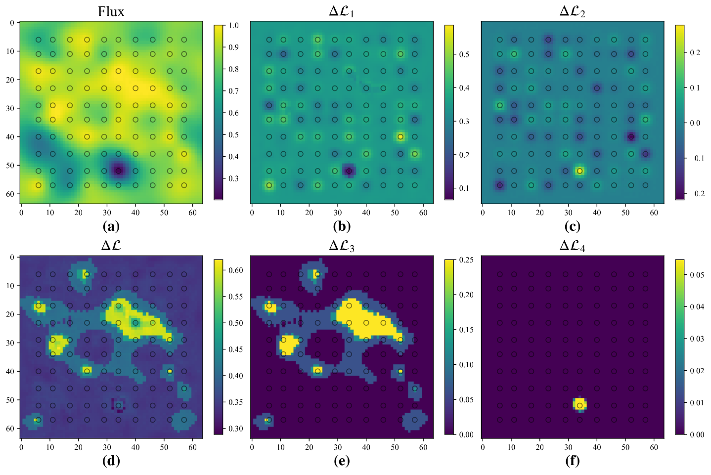
In order to propagate uncertainties to whatever analysis the tomographic map will be used for we need to understand the error properties of our map. Since we have a complete likelihood, it is easy to test the relative likelihood of a given flux realization. The errors will be correlated, as the signal covariance term forces the reconstructed map to be smooth. If we are interested in a pixel by pixel flux error we can calculate this via a response formalism; i.e. by varying each pixel we can study the change in the resulting likelihood. In order to know how the loss function responds, we separate the in Eq. 3 into 4 terms ():
| (A1) |
We add a small increment to the flux at every pixel and see how the value of each term change to penalize the optimization. Figure 10 shows the flux field and the change of loss function and its four components at a slice perpendicular to the LOSs, added 0.1 to the flux at each pixel. We can see in (b) and (c) that the pixels on skewers are the most important ones with the biggest impact on the first two terms compared to other pixels off the skewers, which is expected in standard Wiener Filter as it uses information around skewers. We see the effect of ORCA in (e) and (f) where we add two constraints to the optimization. In (e) we see that works when flux values exceeding one and the yellow and light blue regions can correspond to high flux region in (a). With such a constraint, we could avoid the non-physical values in our final optimized map. In (f) we see that works at low flux region, and it penalizes the optimization when we lose some low flux values, which helps us better recover overdensity. It can also prove that the optimization has reached the minimum of where any increment to flux will increase the total loss function, shown in (d) where all are positive.
Appendix B The choice of parameters in loss function
To explain how we choose parameters in ORCA, we run the mock survey again with the same properties discussed above. works as adding smoothing to the output field, and it is chosen empirically to make the field looks less noisy. We find works best for the S/N and mean sightline spacing in our problem. We use the term with aiming at penalizing the optimization for transmitted flux values above one. Nevertheless, it also impacts the optimization for somehow reducing the low flux values which correspond to overdensity. To compensate for overdensity in the map, we add terms with and . We keep , varying and to illustrate their contributions to the field. At the left panel of Figure 11, we could see that the ORCA optimized transmitted flux field with (cyan) underestimates the overdensity below , compared to the true transmission field from Nyx simulations (black). While with , the ORCA optimized field gets compensated for overdensities, which can be seen on both left and right panel of Figure 11. The choice of and is also empirical, and they should not weigh too high in the loss function as the first two terms are more important in reconstructing the field. We find it useful to set an order magnitude smaller than , and an order magnitude smaller than . We choose to a transmitted flux value where we start to underestimate the transmission. We finally use the parameters which make the reconstructed flux PDF matches best with the true flux in Nyx simulation, and apply them to both mock surveys and real observations. One could expect to alter those parameters depending on the specific problems considered. E.g., the true transmitted flux evolves with redshift changing the PDF of true flux, and we should test where we may underestimate the flux as to pick up a different at different redshifts. Also, when using a different resolution, sightline spacing or , the reconstructed flux PDF could be altered, and a different is needed to decide where to compensate.
Appendix C robustness
To test our algorithm’s robustness, we run the ORCA reconstruction varying the mean sightline spacing and S/N using fixed parameters and . We first vary S/N from 1 to 9 (the same S/N for all skewers in one mock) with a constant Mpc. We then vary from 1 to Mpc with the same S/N distribution as in N-PFS mock. At the left panel of Figure 12, we find that the quality of reconstructed flux PDF matches true PDF increasingly better as we increase the S/N. ORCA performs well when , while we still get reasonably good results with . At the right panel of Figure 12, we find ORCA works well with all tested except for Mpc, whose sightlines are too sparsely sampled.
We find ORCA is robust with parameters we choose in this paper, as the flux PDF will not be influenced much and we still get reasonable map quality when using different sightline spacing and S/N at fixed parameters. We only need to adjust those parameters around the ones we give in this paper for different problems to get optimal results, without searching for parameters in a wide range.
References
- Almgren et al. (2013) Almgren, A. S., Bell, J. B., Lijewski, M. J., Lukić, Z., & Andel, E. V. 2013, The Astrophysical Journal, 765, 39, doi: 10.1088/0004-637x/765/1/39
- Bond et al. (1998) Bond, J. R., Jaffe, A. H., & Knox, L. 1998, Phys. Rev. D, 57, 2117, doi: 10.1103/PhysRevD.57.2117
- Bos et al. (2012) Bos, E. P., van de Weygaert, R., Dolag, K., & Pettorino, V. 2012, Monthly Notices of the Royal Astronomical Society, 426, 440
- Cai et al. (2016) Cai, Z., Fan, X., Peirani, S., et al. 2016, ApJ, 833, 135, doi: 10.3847/1538-4357/833/2/135
- Cai et al. (2017) Cai, Z., Fan, X., Bian, F., et al. 2017, The Astrophysical Journal, 839, 131, doi: 10.3847/1538-4357/aa6a1a
- Caucci et al. (2008) Caucci, S., Colombi, S., Pichon, C., et al. 2008, MNRAS, 386, 211, doi: 10.1111/j.1365-2966.2008.13016.x
- Chiang et al. (2014) Chiang, Y.-K., Overzier, R., & Gebhardt, K. 2014, The Astrophysical Journal, 782, L3, doi: 10.1088/2041-8205/782/1/l3
- Contarini et al. (2020) Contarini, S., Marulli, F., Moscardini, L., et al. 2020, arXiv e-prints, arXiv:2009.03309. https://arxiv.org/abs/2009.03309
- Croft et al. (1998) Croft, R. A. C., Weinberg, D. H., Katz, N., & Hernquist, L. 1998, ApJ, 495, 44, doi: 10.1086/305289
- Eisenstein et al. (2011) Eisenstein, D. J., Weinberg, D. H., Agol, E., et al. 2011, The Astronomical Journal, 142, 72, doi: 10.1088/0004-6256/142/3/72
- Fang et al. (2019) Fang, Y., Hamaus, N., Jain, B., et al. 2019, MNRAS, 490, 3573, doi: 10.1093/mnras/stz2805
- Feng et al. (2019) Feng, Y., Chu, M.-Y., Seljak, U., & McDonald, P. 2019, FastPM: Scaling N-body Particle Mesh solver. http://ascl.net/1905.010
- Forero-Romero et al. (2009) Forero-Romero, J, E., Hoffman, Y., Gottlöber, S. J., Klypin, A., & Yepes, G. 2009, MNRAS, 396, 127, doi: 10.1111/j.1365-2966.2009.14885.x
- Gunn & Peterson (1965) Gunn, J. E., & Peterson, B. A. 1965, ApJ, 142, 1633, doi: 10.1086/148444
- Horowitz et al. (2019) Horowitz, B., Lee, K.-G., White, M., Krolewski, A., & Ata, M. 2019, The Astrophysical Journal, 887, 61, doi: 10.3847/1538-4357/ab4d4c
- Horowitz et al. (2019) Horowitz, B., Seljak, U., & Aslanyan, G. 2019, J. Cosmology Astropart. Phys, 2019, 035, doi: 10.1088/1475-7516/2019/10/035
- Horowitz et al. (2020) Horowitz, B., Zhang, B., Lee, K.-G., & Kooistra, R. 2020, TARDIS Paper II: Synergistic Density Reconstruction from Lyman-alpha Forest and Spectroscopic Galaxy Surveys with Applications to Protoclusters and the Cosmic Web. https://arxiv.org/abs/2007.15994
- Kreisch et al. (2019) Kreisch, C. D., Pisani, A., Carbone, C., et al. 2019, MNRAS, 488, 4413, doi: 10.1093/mnras/stz1944
- Krolewski et al. (2018) Krolewski, A., Lee, K.-G., White, M., et al. 2018, The Astrophysical Journal, 861, 60, doi: 10.3847/1538-4357/aac829
- Lee & Park (2009) Lee, J., & Park, D. 2009, The Astrophysical Journal Letters, 696, L10
- Lee et al. (2014a) Lee, K.-G., Hennawi, J. F., White, M., Croft, R. A. C., & Ozbek, M. 2014a, The Astrophysical Journal, 788, 49, doi: 10.1088/0004-637x/788/1/49
- Lee & White (2016) Lee, K.-G., & White, M. 2016, The Astrophysical Journal, 831, 181, doi: 10.3847/0004-637x/831/2/181
- Lee et al. (2014b) Lee, K.-G., Hennawi, J. F., Stark, C., et al. 2014b, The Astrophysical Journal, 795, L12, doi: 10.1088/2041-8205/795/1/l12
- Lee et al. (2018) Lee, K.-G., Krolewski, A., White, M., et al. 2018, The Astrophysical Journal Supplement Series, 237, 31, doi: 10.3847/1538-4365/aace58
- Liu et al. (2020) Liu, Y., Yu, Y., Yu, H.-R., & Zhang, P. 2020, Phys. Rev. D, 101, 063515, doi: 10.1103/PhysRevD.101.063515
- Mao et al. (2017) Mao, Q., Berlind, A. A., Scherrer, R. J., et al. 2017, The Astrophysical Journal, 835, 161
- Modi et al. (2020) Modi, C., Lanusse, F., & Seljak, U. 2020, FlowPM: Distributed TensorFlow Implementation of the FastPM Cosmological N-body Solver. https://arxiv.org/abs/2010.11847
- Newman et al. (2020) Newman, A. B., Rudie, G. C., Blanc, G. A., et al. 2020, The Astrophysical Journal, 891, 147, doi: 10.3847/1538-4357/ab75ee
- Ozbek et al. (2016) Ozbek, M., Croft, R. A. C., & Khandai, N. 2016, Monthly Notices of the Royal Astronomical Society, 456, 3610, doi: 10.1093/mnras/stv2894
- Perico et al. (2019) Perico, E. L. D., Voivodic, R., Lima, M., & Mota, D. F. 2019, A&A, 632, A52, doi: 10.1051/0004-6361/201935949
- Pichon et al. (2001) Pichon, C., Vergely, J. L., Rollinde, E., Colombi, S., & Petitjean, P. 2001, MNRAS, 326, 597, doi: 10.1046/j.1365-8711.2001.04595.x
- Porqueres et al. (2019) Porqueres, N., Jasche, J., Lavaux, G., & Enßlin, T. 2019, A&A, 630, A151, doi: 10.1051/0004-6361/201936245
- Ravoux et al. (2020) Ravoux, C., Armengaud, E., Walther, M., et al. 2020, Journal of Cosmology and Astroparticle Physics, 2020, 010, doi: 10.1088/1475-7516/2020/07/010
- Reddy et al. (2008) Reddy, N. A., Steidel, C. C., Pettini, M., et al. 2008, The Astrophysical Journal Supplement Series, 175, 48, doi: 10.1086/521105
- Seljak et al. (2017) Seljak, U., Aslanyan, G., Feng, Y., & Modi, C. 2017, Journal of Cosmology and Astroparticle Physics, 2017, 009–009, doi: 10.1088/1475-7516/2017/12/009
- Skibba et al. (2009) Skibba, R. A., Bamford, S. P., Nichol, R. C., et al. 2009, MNRAS, 399, 966, doi: 10.1111/j.1365-2966.2009.15334.x
- Stark et al. (2015a) Stark, C. W., Font-Ribera, A., White, M., & Lee, K.-G. 2015a, MNRAS, 453, 4311, doi: 10.1093/mnras/stv1868
- Stark et al. (2015b) Stark, C. W., White, M., Lee, K.-G., & Hennawi, J. F. 2015b, MNRAS, 453, 311, doi: 10.1093/mnras/stv1620
- Takada et al. (2014) Takada, M., Ellis, R. S., Chiba, M., et al. 2014, PASJ, 66, R1, doi: 10.1093/pasj/pst019
- Tegmark (1997) Tegmark, M. 1997, Physical Review D, 55, 5895
- Tegmark et al. (1998) Tegmark, M., Hamilton, A. J. S., Strauss, M. A., Vogeley, M. S., & Szalay, A. S. 1998, ApJ, 499, 555, doi: 10.1086/305663
- Tran et al. (2010) Tran, K.-V. H., Papovich, C., Saintonge, A., et al. 2010, ApJ, 719, L126, doi: 10.1088/2041-8205/719/2/L126
- Van De Weygaert & Platen (2011) Van De Weygaert, R., & Platen, E. 2011, International Journal of Modern Physics: Conference Series, 01, 41, doi: 10.1142/S2010194511000092
- Vogeley & Szalay (1996) Vogeley, M. S., & Szalay, A. S. 1996, arXiv preprint astro-ph/9601185
- Wake et al. (2005) Wake, D. A., Collins, C. A., Nichol, R. C., Jones, L. R., & Burke, D. J. 2005, ApJ, 627, 186, doi: 10.1086/430117
- Zhang et al. (2020) Zhang, G., Li, Z., Liu, J., et al. 2020, Phys. Rev. D, 102, 083537, doi: 10.1103/PhysRevD.102.083537