Fractal defect states in the Hofstadter butterfly
Abstract
We investigate the electronic properties in the Bloch electron on a square lattice with vacancies in the uniform magnetic field. We show that a single vacancy site introduced to the system creates a defect energy level in every single innumerable fractal energy gap in the Hofstadter butterfly. The wavefunctions of different defect levels have all different localization lengths depending on their fractal generations, and they can be described by a single universal function after an appropriate fractal scaling. We also show that each defect state has its own characteristic orbital magnetic moment, which is exactly correlated to the gradient of the energy level in the Hofstadter diagram. Probing the spatial nature of the defect-localized states provides a powerful way to elucidate the fractal nature of the Hofstadter butterfly.
Introduction
The Hofstadter butterfly is the energy spectrum of Bloch electrons moving in a two-dimensional lattice under a uniform magnetic field, which is characterized by a nested fractal band structure Harper 1955a; Harper 1955b; Zak 1964; Azbel 1964; Hofstadter 1976; Wannier 1978; Wannier et al. 1979. It has been actively studied in condensed matter physics Claro and Wannier 1979; Rammal 1985; Pfannkuche and Gerhardts 1992; Gumbs et al. 1995; Koshino et al. 2001; Xiao et al. 2003, and also from a wide variety of perspectives including mathematics Bellissard; Helffer and Sj€ostrand 1988; Last 1994; Prodan 2015; Ikeda 2018a; Ikeda 2018b; Ikeda 2018c and quantum geometry Hatsuda et al. 2016; Duan et al. 2018. Experimentally, the evidence of the fractal nature of the Hofstadter spectrum was found in various systems, such as GaAs/AlGaAs heterostructures with superlattices Schlösser et al. 1996; Albrecht et al. 2001; Geisler et al. 2004, ultracold atoms in optical lattices Jaksch and Zoller 2003; Aidelsburger et al. 2013; Miyake et al. 2013, graphene-based moiré superlattices Dean et al. 2013; Hunt et al. 2013; Ponomarenko et al. 2013, photons with the superconducting qubits Roushan et al. 2017 and one-dimensional acoustic array Kuhl and Stöckmann 1998; Richoux and Pagneux 2002; Ni et al. 2019.
Currently, however, the experimental observation of the butterfly is mostly limited to the measurement of the spectral structure and the transport properties. Actually, richer fractal information is encoded in the wavefunctions of the Hofstadter butterfly, but it is generally considered to be difficult to access in experiments. The characteristic spatial property of each wavefunction is generally averaged out in the physical observables due to the summation over the Bloch momentum.
In this paper, we theoretically propose that the spatial structure in the Hofstadter system can be elucidated by introducing a point defect to the system. In an electron system under a magnetic field, generally, a point disorder potential gives rise to defect localized states in the energy gaps between Landau levels Ando and Uemura 1974; Ando 1974; Ando et al. 1975; Prange 1981; Joynt and Prange 1984; Gredeskul et al. 1997; Niimi et al. 2006. The effect of lattice defects on the Hofstadter spectrum was investigated in some past works Pereira and Schulz 2008; İslamoğlu et al. 2012; İslamoğlu et al. 2012; Pedersen and Pedersen 2013; Zhou et al. 2005; Grishanov and Popov 2018; Matsuki and Ikeda 2019; Diop et al. 2020, and the in-gap defect levels were found at a certain magnetic flux Diop et al. 2020. However, it has not been clear how the self-similar nature is manifested in the defect localized states.
In this letter, we study the Hofstadter problem with vacancy defects in a square lattice to investigate the fractal properties of defect states. We show that a single vacancy site introduced to the system creates a defect energy level in every single innumerable fractal energy gap in the Hofstadter butterfly. We find that the wavefunctions of different defect levels have all different localization lengths depending on their fractal generations, and importantly, the localization length of any levels can be approximately described by a single universal curve after an appropriate fractal scaling. We also find that the defect states are accompanied by an orbital magnetic moment due to rotating electric current, and its magnitude exactly coincides with the gradient of the energy gap in the Hofstadter diagram. These results give a new quantitative perspective on the spatial fractal nature of the Hofstadter butterfly, and provide a powerful way to elucidate the fractal nature of the Hofstadter butterfly by probing the defect states.

Formulation
We consider a square lattice with a single-site defect as illustrated in Fig. 1. We assume that the system is periodic with supercell and each supercell includes a single vacancy site. The system is under a uniform magnetic field perpendicular to the system. Let be the number of magnetic flux quanta per a plaquette, where is the spacing between the lattice points. In what follows, we consider a single orbital tight-binding Hamiltonian,
| (1) |
where is the hopping parameter, is a pair of the nearest neighbor sites, is the creation (annihilation) operator at site , is the site of defects, is the Peierls phase Peierls 1933, and is the vector potential. We take throughout this letter. In a perfect lattice without a defect under a rational magnetic flux (: coprime integers), the energy band splits into subbands Hofstadter 1976.
The number of total magnetic fluxes penetrating an entire supercell is . For with co-prime integers and , the eigenstates of the system can be taken as magnetic Bloch states, which satisfy the following conditions Zak 1964; Xiao et al. 2010; Moon and Koshino 2012:
| (2) | |||||
| (3) |
where and are the primitive lattice vectors of the magnetic unit cell. Then the eigen-energies and eigen-wavefunctions can be obtained by diagonalizing Hamiltonian matrix. We also perform similar calculation and analyses for a honeycomb lattice with periodic vacancies, which is presented in Supplementary Information.
Fractal defect states
Fig. 2(a) shows the energy spectrum of superlattice with a single-site defect, plotted against the magnetic flux . The red and black dots represent the bulk states and the defect-localized states, respectively. Here the defect-localized states are identified by the condition that the wave amplitude within seven-site distance from the defect point is more than of the total amplitude. We observe that a defect level exists in every single gap, indicating that the spectrum of the defect states inherits the nested fractal structure of the Hofstadter butterfly.
The left panels in Fig. 3 represent the squared wavefunctions of defect levels (i), (ii) and (iii) in Fig. 2, which are taken from different minigaps of the Hofstadter butterfly. Here the eigenstates are calculated for superlattice, where the overlap between defect states in neighboring unit cells is sufficiently small. We clearly observe that the defect-state wavefunctions all localize around the vacancy, while their characteristic length scales are completely different. Actually, as shown in the following, the localization length of the defect states is a good quantitative indicator of the fractal generation of the minigap.
To demonstrate this, we first introduce an addressing rule for the fractal structure Hofstadter 1976; MacDonald 1983. As shown in Fig. 2(b), the whole energy spectrum in (referred to as the main spectrum in the following) can be divided into left, right, center subcells, which are labelled by , and , respectively. The gap structure of each subcell plotted against the local variable is identical to that of the main spectrum plotted against the magnetic flux . The global variable and the local variable for the subcell are related by , where
| (4) | ||||
| (5) |
In Fig. 2(b), we present an axis of the local variable for subcell, where correspond to , respectively. The main spectrum can also be regarded as a single subcell, where the local variable is the magnetic flux itself, i.e., . By repeating this addressing scheme, we can define subcells in higher generations. For instance, refers to subcell in subcell in the main spectrum. The relation between the local variable for subcell and the global variable is given by .
For each subcell, we define the positive (negative) principal gap as the diagonal gap running from the lower (upper) left corner to the upper (lower) right corner of the subcell plotted against . Any gap in the Hofstadter diagram can be uniquely identified as the positive or negative principal gap of a specific subcell or of the main spectrum.

In the following, we compare the localization lengths of the corresponding defect states in the principal gaps of different subcells, which share the same local variable . The defect levels (i), (ii) and (iii) in Figs. 2 and 3 are actually taken from the positive principal gaps of the main spectrum, and , respectively, with the same local variable . The global variables for (i), (ii) and (iii) are , and , respectively. For each state, we define the localization length by , where is the wave amplitude at site , and is the vacancy position. Here we show that the ratio of ’s of different subcells is approximately equal to the ratio of the denominators of of those states. For the states (i), (ii) and (iii) in Fig. 3, for instance, this claims that the ratio of the ’s of the three states is . Indeed, it approximates the ratio of the numerically calculated values , respectively (indicated by radii of circles in Fig. 3). The reason for this scaling rule can be understood by considering an ideal system without defects. Specifically, the Schrödinger equation for the ideal square lattice with is reduced to a one-dimensional Harper’s equation with the spatial period of Harper 1955b; Hofstadter 1976. The period works as the reference length scale to compare the wavefunctions in different fractal levels; for example, an eigenstate of Harper’s equation at and the corresponding state of cell at have similar structures with length scales of . Naturally, the defect states take over the same scaling feature.
Let be the localization length of the defect state in the principal gap of the main spectrum at the flux , and be that of subcell at local variable . According to the argument above, we have the relation , where is the denominator of . Using Eqs. (4) and (5), this immediately leads to the relation between and ,
| (6) | |||
| (7) |
which is a key finding of this work. Note that, although the denominator is not a continuous function of , the scaling ratio is a continuous function of . Similarly, the relation for higher fractal generations can be obtained from . For subcell, for instance, it gives .
In Fig. 4 , we plot (a) the localization lengths and (b) the renormalized values as functions of the local variable . Here the solid and dashed curves represent the positive and negative principal gaps, respectively. The two curves are identical for the main spectrum due to the electron-hole symmetry. We see that the renormalized localization lengths [Fig. 4(b)] quantitatively match in a wide range of . The diverges at in proportion to , corresponding to the fact that the length scale in a weak magnetic field is given by the magnetic length . We have the same feature in symmetrically. At , we notice that the diverges only in the negative gaps of the subcells, while it remains finite in the positive gaps. This links to the fact that the negative gaps close while the positive gaps are open at . For the main spectrum and any subcells centered at , the positive and negative gaps both closes at at the same time because of the electron-hole symmetry, and the localization lengths both diverge accordingly. In Fig. 4(b), the negative gaps of and seem to follow a different curve from the rest in the limit of , and this is related to the fact that the gap is approaching the Dirac point of the magnetic Bloch band at . The origin of the different scaling nature is argued in Supplemental Information.
Magnetic moment
Generally, the in-gap defect states in a time-reversal-symmetry broken system are accompanied by an orbital current circulation Jha et al. 2017; Diop et al. 2020. Here we find that the magnetic moment created by the orbital current of the defect states in our system is precisely related to the gradient of fractal defect states on the Hofstadter diagram. The local electric current from site to site is calculated by
| (8) |
The right column in Fig. 3 shows that the local current calculated for the defect states (i), (ii) and (iii). The thickness of and the size of arrows is proportional to the absolute value of current. Here the current rotates in the clockwise direction, i.e., it has a negative magnetic moment. Actually, the direction of the current synchronizes with the gradient of the defect energy level in the Hofstadter diagram, because the orbital magnetic moment is given by (see Supplementary Information for the proof). In other words, a defect state in the Hofstadter butterfly precisely tunes its own current circulation, in such a way that the energy level stays inside the fractal gap in changing magnetic field.

Multi-point vacancies
We also consider various multi-point vacancies in Fig. 5; (a) consecutive two-point defect and (b) three-point defect. The corresponding spectra of superlattice are shown in Fig. 5, where we observe that the number of defect states in every single fractal gap matches that of the missing sites in the defect. When the number of missing atoms becomes larger, we expect that more and more defect levels fill in the energy gaps, and they eventually form quantum Hall edge states circulating around the hole. The fractal defect levels can be regarded as the quantized version of the quantum Hall edge state in the atomic limit. Therefore the emergence of the defect levels in the fractal gaps may be viewed as a sort of the bulk-edge correspondence Hatsugai 1993a; Hatsugai 1993b requiring the existence of the edge states in a bulk gap with a non-zero Chern number. However, it should also be noted that the number of the defect states in each gap is not at all related to the Chern number, but it just coincides with the number of missing sites for any gaps.
Conclusion and Discussions
We have reported that the states localized around the defects fractally appear in every single band gap of the Hofstadter butterfly. The defect states in different energy gaps have all different length scale in the spatial decay, while they follow a universal curve after the appropriate fractal scaling. Each defect state has its own characteristic magnetic moment, which is exactly linked to the gradient of the corresponding bulk energy gap in the Hofstadter diagram.
While the previous observations of Hofstadter butterfly have been mainly conducted by spectroscopic/transport measurements of the energy gap structure, our work provides a powerful method to observe the fractal nature in the wavefunction by measuring the spatial decay of the defect states using scanning tunneling spectroscopy.
Acknowledgement
We thank Kin-ya Oda for fruitful discussions. This work was supported in part by Grant-in-Aid for JSPS Research Fellow, No. JP19J20559, JP19J11073, JSPS KAKENHI Grant Number JP20H01840 and JP20H00127 and by JST CREST Grant Number JPMJCR20T3, Japan.
References
- Harper (1955a) P. G. Harper, Proceedings of the Physical Society. Section A 68, 879 (1955a).
- Harper (1955b) P. G. Harper, Proceedings of the Physical Society. Section A 68, 874 (1955b).
- Zak (1964) J. Zak, Phys. Rev. 134, A1602 (1964).
- Azbel (1964) M. Y. Azbel, Zh. Eksp. Teor. Fiz. 46, 929 (1964).
- Hofstadter (1976) D. R. Hofstadter, Phys. Rev. B 14, 2239 (1976).
- Wannier (1978) G. H. Wannier, physica status solidi (b) 88, 757 (1978).
- Wannier et al. (1979) G. H. Wannier, G. M. Obermair, and R. Ray, physica status solidi (b) 93, 337 (1979).
- Claro and Wannier (1979) F. H. Claro and G. H. Wannier, Phys. Rev. B 19, 6068 (1979).
- Rammal (1985) R. Rammal, J. Phys. France 46, 1345 (1985).
- Pfannkuche and Gerhardts (1992) D. Pfannkuche and R. R. Gerhardts, Phys. Rev. B 46, 12606 (1992).
- Gumbs et al. (1995) G. Gumbs, D. Miessein, and D. Huang, Phys. Rev. B 52, 14755 (1995).
- Koshino et al. (2001) M. Koshino, H. Aoki, K. Kuroki, S. Kagoshima, and T. Osada, Phys. Rev. Lett. 86, 1062 (2001).
- Xiao et al. (2003) Y. Xiao, V. Pelletier, P. M. Chaikin, and D. A. Huse, Phys. Rev. B 67, 104505 (2003).
- (14) J. Bellissard, Operator Algebras and Application, edited by D. E. Evans and M. Takesaki (Cambridge University Press, Cambridge, England, 1988), Vol. 2 .
- Helffer and Sj€ostrand (1988) B. Helffer and J. Sj€ostrand, Suppl. Bull. Soc. Math. France 116(4) (1988).
- Last (1994) Y. Last, Commun.Math. Phys. 164, 421–432 (1994).
- Prodan (2015) E. Prodan, Phys. Rev. B 91, 245104 (2015).
- Ikeda (2018a) K. Ikeda, Journal of Mathematical Physics 59, 061704 (2018a).
- Ikeda (2018b) K. Ikeda, Annals Phys. 397, 136 (2018b).
- Ikeda (2018c) K. Ikeda, (2018c), arXiv:1812.11879 [cond-mat.mes-hall] .
- Hatsuda et al. (2016) Y. Hatsuda, H. Katsura, and Y. Tachikawa, New J. Phys. 18, 103023 (2016), arXiv:1606.01894 [hep-th] .
- Duan et al. (2018) Z. Duan, J. Gu, Y. Hatsuda, and T. Sulejmanpasic, ArXiv e-prints (2018), arXiv:1806.11092 [hep-th] .
- Schlösser et al. (1996) T. Schlösser, K. Ensslin, J. P. Kotthaus, and M. Holland, Semiconductor Science and Technology 11 (1996).
- Albrecht et al. (2001) C. Albrecht, J. H. Smet, K. von Klitzing, D. Weiss, V. Umansky, and H. Schweizer, Phys. Rev. Lett. 86, 147 (2001).
- Geisler et al. (2004) M. Geisler, J. Smet, V. Umansky, K. Von Klitzing, B. Naundorf, R. Ketzmerick, and H. Schweizer, Phys. Rev. Lett. 92, 256801 (2004).
- Jaksch and Zoller (2003) D. Jaksch and P. Zoller, New Journal of Physics 5, 56 (2003).
- Aidelsburger et al. (2013) M. Aidelsburger, M. Atala, M. Lohse, J. T. Barreiro, B. Paredes, and I. Bloch, Phys. Rev. Lett. 111, 185301 (2013).
- Miyake et al. (2013) H. Miyake, G. A. Siviloglou, C. J. Kennedy, W. C. Burton, and W. Ketterle, Phys. Rev. Lett. 111, 185302 (2013).
- Dean et al. (2013) C. R. Dean, L. Wang, P. Maher, C. Forsythe, F. Ghahari, Y. Gao, J. Katoch, M. Ishigami, P. Moon, M. Koshino, T. Taniguchi, K. Watanabe, K. L. Shepard, J. Hone, and P. Kim, Nature 497, 598–602 (2013).
- Hunt et al. (2013) B. Hunt, J. D. Sanchez-Yamagishi, A. F. Young, M. Yankowitz, B. J. LeRoy, K. Watanabe, T. Taniguchi, P. Moon, M. Koshino, P. Jarillo-Herrero, and R. C. Ashoori, Science 340 (2013), 10.1126/science.1237240.
- Ponomarenko et al. (2013) L. A. Ponomarenko, R. V. Gorbachev, G. L. Yu, D. C. Elias, R. Jalil, A. A. Patel, A. Mishchenko, A. S. Mayorov, C. R. Woods, J. R. Wallbank, M. Mucha-Kruczynski, B. A. Piot, M. Potemski, I. V. Grigorieva, K. S. Novoselov, F. Guinea, V. I. Fal’ko, and A. K. Geim, Nature 497, 594 (2013).
- Roushan et al. (2017) P. Roushan, C. Neill, J. Tangpanitanon, V. M. Bastidas, A. Megrant, R. Barends, Y. Chen, Z. Chen, B. Chiaro, A. Dunsworth, A. Fowler, B. Foxen, M. Giustina, E. Jeffrey, J. Kelly, E. Lucero, J. Mutus, M. Neeley, C. Quintana, D. Sank, A. Vainsencher, J. Wenner, T. White, H. Neven, D. G. Angelakis, and J. Martinis, Science 358, 1175 (2017).
- Kuhl and Stöckmann (1998) U. Kuhl and H.-J. Stöckmann, Phys. Rev. Lett. 80, 3232 (1998).
- Richoux and Pagneux (2002) O. Richoux and V. Pagneux, Europhysics Letters (EPL) 59, 34 (2002).
- Ni et al. (2019) X. Ni, K. Chen, M. Weiner, D. J. Apigo, C. Prodan, A. Alù, E. Prodan, and A. B. Khanikaev, Commun Phys 2, 256 (2019).
- Ando and Uemura (1974) T. Ando and Y. Uemura, Journal of the Physical Society of Japan 36, 959 (1974).
- Ando (1974) T. Ando, Journal of the Physical Society of Japan 37, 622 (1974).
- Ando et al. (1975) T. Ando, Y. Matsumoto, and Y. Uemura, Journal of the Physical Society of Japan 39, 279 (1975).
- Prange (1981) R. E. Prange, Phys. Rev. B 23, 4802 (1981).
- Joynt and Prange (1984) R. Joynt and R. E. Prange, Phys. Rev. B 29, 3303 (1984).
- Gredeskul et al. (1997) S. Gredeskul, M. Zusman, Y. Avishai, and M. Azbel’, Physics Reports 288, 223 (1997).
- Niimi et al. (2006) Y. Niimi, H. Kambara, T. Matsui, D. Yoshioka, and H. Fukuyama, Phys. Rev. Lett. 97, 236804 (2006).
- Pereira and Schulz (2008) A. L. C. Pereira and P. A. Schulz, Phys. Rev. B 78, 125402 (2008).
- İslamoğlu et al. (2012) S. İslamoğlu, M. O. Oktel, and O. Gülseren, Journal of Physics: Condensed Matter 24, 345501 (2012).
- İslamoğlu et al. (2012) S. İslamoğlu, M. O. Oktel, and O. b. u. Gülseren, Phys. Rev. B 85, 235414 (2012).
- Pedersen and Pedersen (2013) J. G. Pedersen and T. G. Pedersen, Phys. Rev. B 87, 235404 (2013).
- Zhou et al. (2005) C. Zhou, M. Berciu, and R. N. Bhatt, Phys. Rev. B 71, 125310 (2005).
- Grishanov and Popov (2018) E. N. Grishanov and I. Y. Popov, Russ. J. Math. Phys. 25, 277–283 (2018).
- Matsuki and Ikeda (2019) Y. Matsuki and K. Ikeda, Journal of Physics Communications 3, 055003 (2019).
- Diop et al. (2020) S.-S. Diop, L. Fritz, M. Vojta, and S. Rachel, Phys. Rev. B 101, 245132 (2020).
- Peierls (1933) R. Peierls, Zeitschrift für Physik 80, 763 (1933).
- Xiao et al. (2010) D. Xiao, M.-C. Chang, and Q. Niu, Rev. Mod. Phys. 82, 1959 (2010).
- Moon and Koshino (2012) P. Moon and M. Koshino, Phys. Rev. B 85, 195458 (2012).
- MacDonald (1983) A. H. MacDonald, Phys. Rev. B 28, 6713 (1983).
- Jha et al. (2017) V. B. Jha, G. Rani, and R. Ganesh, Phys. Rev. B 95, 115434 (2017).
- Hatsugai (1993a) Y. Hatsugai, Phys. Rev. Lett. 71, 3697 (1993a).
- Hatsugai (1993b) Y. Hatsugai, Phys. Rev. B 48, 11851 (1993b).
Supplemental Information for: Fractal defect states
in the Hofstadter butterfly
Yoshiyuki Matsuki,1 Kazuki Ikeda,1 and Mikito Koshino1
1Department of Physics, Osaka University, Toyonaka, Osaka 560-0043, Japan
I The origin of unusual scaling curves of localization length
In the main article, we demonstrated that the localization length of defect state in each minigap of the Hofstadter butterfly is approximately described by a single universal function when it is appropriately scaled. However, there are some exceptional gaps in the spectrum, where the localization length follows a different curve.
An exceptional scaling behavior occurs in the principal gaps of any subcells ending with , i.e., . Figure 6(a) shows the renormalized localization length [Eqs. (6) and (7) of the main text] of the positive principal gap of the main cell, , and subcells [, , , ] as functions of the local variable . We observe that the curves slightly shift in relative to each other in the limit of , whereas they precisely match in .
The reason for the deviation can be understood as follows. In the weak magnetic field limit, the principal gaps of , and subcell correspond to the second, third and fourth lowest gaps of the Landau-level spectrum, respectively [Fig. 6(c)]. This is in contrast to any subcells NOT ending with , where the principal gap definitely connects to the lowest gap (the gap just above the lowest Landau level) in the magnetic Bloch subband at . The characteristic length scale of the -th Landau level wavefunction is given by , where is the magnetic length. Accordingly, the defect-localized state which exists between the Landau levels and should have the length scale of the order of , and the dependence on results in the different scaling curves. Indeed, the localization lengths of the main cell, , ,and in the region of in Fig. 6(a) are very well (within 1%) fitted by
| (9) |
with and , respectively. Here we note that (in units of the lattice constant) in this region.
Similarly, the same scaling rule is applicable to subcells. In Fig. 6(b), we plot the renormalized localization length of the principal gaps of , and subcells by dashed curves. In the limit , the three curves perfectly match with those of the main cell, and , respectively (solid curves).
Another exceptional case occurs in a gap connected to the Dirac point of the magnetic Bloch band, such as the negative principal gaps of and mentioned in the main text. If we take subcell, for instance, the gap leads to the point of and of the main diagram in the limit of , where a pair of magnetic Bloch bands are touching just like in graphene due to the electron-hole symmetry of the model. Now the wavefunction of the Landau level in graphene is composed of the and at different sublattices [A1,A2], so that its length scale is just in the middle of those of -th and -th Landau levels in the conventional massive electron. Accordingly, the defect-localized states should have the intermediate localization length compared to the massive system. Indeed, the localization length of defect states in cell for small is given by , which is between the values of and in Eq. (9). In Fig. 4(b) in the main text, we see that the subcell also follows the same curves as . This is because its negative principal gap leads to the point of and , which is also the Dirac point.
II The gradient of defect states and the magnetic moment
We prove that the gradient of a defect energy level in the Hofstadter diagram coincides with the magnetic moment created by the local electric current. For this purpose we show that the magnetic moment obeys Eq. (18) in the presence of a generic potential in quantum mechanics. To show this formula we consider the system described by the Hamiltonian,
| (10) |
Considering a small change in the magnetic field, we obtain the perturbed Hamiltonian
| (12) | |||||
where is the current operator
| (13) |
The variation of the energy within the first order perturbation is
| (14) |
where is the eigenfunction of . The first term in the most right hand side in (14) is evaluated as follows:
| (15) |
We can evaluate the second term in a similar way, and finally obtain
| (16) |
Here we used the local current operator ,
| (17) |
By using the expression of the magnetizing current , one can find that the magnetic moment obeys
| (18) |
III The relationship between the distance of defect sites and the fractal energy spectrum
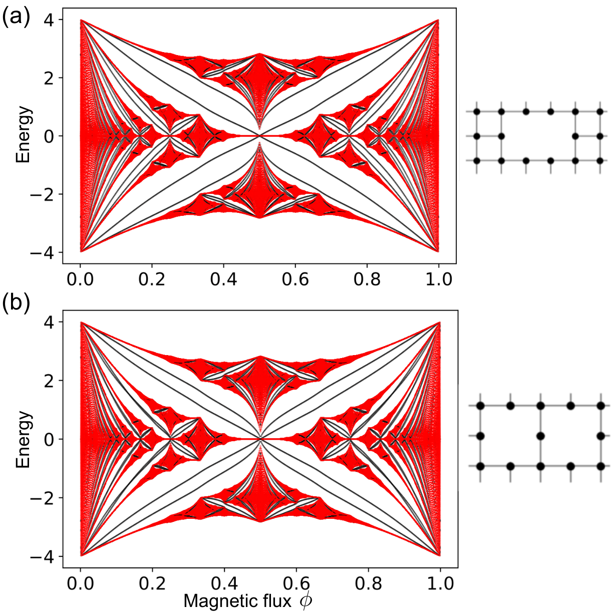
Here we discuss the relationship between the distances of vacancy sites and the fractal energy levels in the Hofstadter diagram. For this purpose, we consider the two-point vacancies illustrated in Fig.7: (a) consecutive two-point defect, (b) two split defects. The corresponding spectra of superlattice are shown in Fig.7(a) and (b). By comparing Figs.7(a) and (b), we notice that the two defect energy levels get closer as the distance between the two defect sites gets further away. This is a consequence of the hybridization of the defect states of two single vacancy sites, where the coupling strength exponentially decreases as the distance increases. A similar effect is also found in defect states in graphene [A3]. We see the same tendency consistently in all the fractal gaps.

III.1 Fractal Structure and Wavefunction on a honeycomb lattice with a defect

Here we consider defect-localized states on a honeycomb superlattice with a single-site defect (Fig. 8). We assume that the system is periodic with supercell and every single supercell includes a single vacancy site. Now we take the super period , which is taken to be sufficiently large to avoid interference between defect-localized states in neighboring cells. The Bloch electron wavefunctions obey the magnetic Bloch condition:
| (19) | |||||
| (20) |
where and are the primitive lattice vectors of the magnetic unit cell.

FIG.9(a) shows the energy spectrum of superlattice in a honeycomb lattice with a single defect, plotted against the magnetic flux . The red and black dots represent the bulk states and the defect-localized states, respectively. Here the defect-localized states are identified by the condition that the wave amplitude within from the defect point is more than of the total amplitude. We observe that a defect level exists in every single gap, indicating that the spectrum of the defect states inherits the nested fractal structure of the Hofstadter butterfly, same as the square lattice case.

To compare uniformly the localization lengths in different fractal generation gaps, we again define the subcell decomposition and the local variable in a honeycomb lattice. As shown in Fig.9(b), the main energy spectrum in includes the self-similar structure subcell . In fact, the gap structure of each subcell plotted against the local variable is identical to that of the main spectrum plotted against the magnetic flux . The relationship between the global variable and local variable is
| (21) |
In the main spectrum, the global variable corresponds to the local variable since the main spectrum can be viewed as a single subcell. In the following, we show the amplitude and the electric current of the corresponding defects states of different subcells at the same local variable .
The left panels in Fig.10 show the distribution of the wave amplitude of three defect levels (i), (ii) and (iii) indicated in Fig. 9, which are taken from the positive principal gaps of the main spectrum, and , respectively, with the same local variable . From the equation (21), the global variables for (i), (ii) and (iii) are , and , respectively. We can observe that the defect wavefunctions localize around the defect with different length scales.
Moreover, the right panels in Fig.10 represent that the local current calculated for the defect states (i), (ii) and (iii). As discussed above, the magnetic moment created by the local current coincides with the gradient on the Hofstadter diagram (Fig.9). Actually, the current rotates in the clockwise direction, and the direction of the current synchronizes with the gradient of the defect energy level in the Hofstadter diagram. The same properties as the square lattice case (the localization around the defect, the fractality of localization length, and the correspondence between magnetic moment and gradient of defect states) are observed in a honeycomb lattice case.
- [A1]
N. H. Shon and T. Ando, Journal of the Physical Society of Japan, 67, 2421-2429 (1998).
- [A2]
Y. Zheng and T. Ando, Phys. Rev. B 65, 245420 (2002).
- [A3]
A. L. C. Pereira and P. A. Schulz, Phys. Rev. B 78, 125402 (2008).