跳到论文正文
W Papers独立论文阅读器 arXiv:2102.12039 论文正文 计算阅读时间 · 0%
引用这篇论文根据当前论文元数据生成,正式投稿前建议核对。


License: arXiv.org perpetual non-exclusive license
arXiv:2102.12039v6 [stat.AP] 19 Feb 2024

Population-level Task-evoked Functional Connectivity
via Fourier Analysis

Kun Meng Affiliation: Division of Applied Mathematics, Brown University, Providence, Rhode Island, USA Affiliation: Correspondence: Kun Meng, e-mail: kun_meng@brown.edu.    Ani Eloyan Affiliation: Department of Biostatistics, Brown University School of Public Health, Providence, Rhode Island, USA
Abstract

Functional magnetic resonance imaging (fMRI) is a non-invasive and in-vivo imaging technique essential for measuring brain activity. Functional connectivity is used to study associations between brain regions, either while study subjects perform tasks or during periods of rest. In this paper, we propose a rigorous definition of task-evoked functional connectivity at the population level (ptFC). Importantly, our proposed ptFC is interpretable in the context of task-fMRI studies. An algorithm for estimating the ptFC is provided. We present the performance of the proposed algorithm compared to existing functional connectivity frameworks using simulations. Lastly, we apply the proposed algorithm to estimate the ptFC in a motor-task study from the Human Connectome Project.

Keywords:11 1 • The project herein was supported by Grant Number 5P20GM103645 from the National Institute of General Medical Sciences. • Abbreviations: BOLD, blood-oxygenation level-dependent; DC, dynamic connectivity; fMRI, functional magnetic resonance imaging; FC, functional connectivity; HCP, Human Connectome Project; HRF, hemodynamic response function; MLM, mixed linear model; ptFC, task-evoked functional connectivity at the population level; ptFCE, ptFC estimation; PH, persistent homology; ROI, region of interest; SBHM, spatial Bayesian hierarchical model; WSMZ, weakly stationary with mean zero. AMUSE algorithm; Human Connectome Project; motor-task; weakly stationary with mean zero.

1 Introduction

Functional magnetic resonance imaging (fMRI) is a non-invasive brain imaging technique used to estimate both brain regional activity and interactions between brain regions. In fMRI studies, brain signals are measured on 3-dimensional volume elements (voxels) during a certain period of time, and each signal is observed at discrete time points, e.g., to investigate neural activity. However, since neural activity occurs in milliseconds, it is impossible to directly observe it using fMRI technology. The neural activity is implicitly captured by blood-oxygenation level-dependent (BOLD) signals. When neural activity in a brain area occurs, it is followed by localized changes in metabolism, where the corresponding local oxygen consumption increases, and then oxygen-rich blood flows to this area. This process results in an increase in oxyhemoglobin and a decrease in deoxyhemoglobin. The BOLD signal value at each time point is the difference between the oxyhemoglobin and deoxyhemoglobin levels. The signal consisting of BOLD values across all time points measures the localized metabolic activity influenced by the local brain vasculature, and it indirectly measures the localized neural activity.

1.1 Goal and Main Contribution

During an fMRI experimental study, subjects either rest (resting-state fMRI) or perform tasks (task-fMRI). We focus on task-fMRI throughout this paper. While the experiment may involve one or multiple tasks, we model the effect of one of the tasks, which is considered the task of interest. In this paper, we propose a framework for modeling the functional connectivity evoked by the single task of interest, referred to as task-evoked functional connectivity, while ignoring the effect of the nuisance tasks.

Dependencies between activation in any two regions of the brain are referred to as functional connectivity (Cribben and Fiecas 2016, FC,). These dependencies have been widely studied, and several approaches have been proposed for the estimation of FC, especially resting-state FC (i.e., the FC derived from resting-state fMRI data). Task-evoked FC is fundamentally different from resting-state FC. Lynch et al. 2018 show that existing estimates of task-evoked FC cannot explain differences between the resting-state FC and the task-evoked FC. While the brain FC in an individual subject is often of interest (referred to as subject-level FC), population-level estimates of FC have been proposed in the literature and used for obtaining more robust subject-level FC estimates (Bowman et al. 2008, Mejia et al. 2018, e.g.,). To overcome the limitations of existing task-evoked FC estimation approaches when investigating population-level FC, we propose a novel definition of population-level task-evoked FC (ptFC). This definition is based on a correlation of subject-specific effects that capture task-evoked neural activity. Importantly, our proposed ptFC framework takes into account the complex biological processes of the brain response to task stimuli that many existing estimators ignore.

Under the model assumption of the Bayesian hierarchical framework proposed by Bowman et al. 2008, our proposed ptFC is equal to their “task-related inter-region functional connectivity.” However, our proposed ptFC and our proposed approach to estimating ptFC do not depend on the referred Bayesian hierarchical framework and work for more general structures (see Section 2.2 for details). Furthermore, with appropriate estimation adjustments, our proposed framework has the potential to be an extension of many existing models for fMRI, particularly the Bayesian models that include grouped random terms representing signals. Bowman 2014 and Zhang et al. 2015 provide thorough reviews of existing Bayesian models for fMRI data. Exploration of applying our framework to the existing models is left for future research.

1.2 Task-fMRI Signal Types

We are interested in modeling neural activity and BOLD signals of a set of subjects ω\omega from a population of interest. At each time point tt, we denote by Yk​(ω,t)Y_{k}(\omega;t) the BOLD signal value at the kt​hk^{th} node of the subject ω\omega’s brain. The word “node” refers to either a voxel or a region of interest (ROI). Aggregated BOLD signals at a macro-area level are often of interest. That is, for each subject, BOLD signals are spatially averaged within each pre-selected ROI, and the resulting ROI-specific signals are analyzed. The BOLD signals for subject ω\omega are represented by a vector-valued function {𝒀⁡(ω,t)=(Y1​(ω,t),⋯,YK​(ω,t))T|t∈𝒯}\{\boldsymbol{Y}(\omega;t)=\left(Y_{1}(\omega;t),\cdots,Y_{K}(\omega;t)\right)^{T}|\,t\in\mathcal{T}\} on 𝒯\mathcal{T}, where 𝒯\mathcal{T} is the collection of time indices and KK is the number of nodes. Furthermore, we assume that 𝒯\mathcal{T} is a compact subset of ℝ\mathbb{R}.

In this paper, we model the following three types of signals in task-fMRI studies:

  1. i

    Stimulus signals, denoted by N⁡(t)N(t), representing the experimental designs of tasks. Specifically, N⁡(t)=1N(t)=1 when the stimulus of interest is present, and N⁡(t)=0N(t)=0 when the stimulus is absent (see Eq. (1.3) for an example). Given a hemodynamic response function (Lindquist et al. 2008, HRF,), a stimulus signal N⁡(t)N(t) determines the design matrix of a general linear model (Friston et al. 1995, GLM,). Further details are provided in Section 2.1.

  2. ii

    Task-evoked neural activity signals at the kt​hk^{th} node, denoted by Φk​[ω;N​(t)]\Phi_{k}[\omega;\,N(t)], stemming solely from the task stimulus N⁡(t)N(t), where the “stimulus-to-activity” maps Φk​[ω;∙]:N⁡(t)↦Φk​[ω;N⁡(t)]\Phi_{k}[\omega;\,\bullet]:\,N(t)\mapsto\Phi_{k}[\omega;\,N(t)] depend on subjects ω\omega. The map Φk​[ω;∙]\Phi_{k}[\omega;\bullet] characterizes how neurons at the kt​hk^{th} node of the subject ω\omega react to stimulus N⁡(t)N(t).

  3. iii

    Observed BOLD signals Yk​(ω,t)=Ψk​{ω;Φk​[ω;N⁡(t)]}Y_{k}(\omega;t)=\Psi_{k}\left\{\omega;\,\Phi_{k}\left[\omega;\,N(t)\right]\right\} that are associated with the task-evoked neural activity Φk​[ω;N​(t)]\Phi_{k}[\omega;\,N(t)], where the “activity-to-BOLD” maps Ψk​{ω;∙}:Φk​[ω;N⁡(t)]↦Yk​(ω,t)\Psi_{k}\{\omega;\bullet\}:\,\Phi_{k}[\omega;N(t)]\mapsto Y_{k}(\omega;t) are ω\omega-dependent. The map Ψk​{ω;∙}\Psi_{k}\{\omega;\bullet\} describes how neural activity Φk​[ω;N​(t)]\Phi_{k}[\omega;N(t)] induces BOLD signal Yk​(ω,t)Y_{k}(\omega;t). A comprehensive discussion on the “activity-to-BOLD” mechanism can be found in Chapter 3 of Ashby 2019.

The relationship between the three types of signals is illustrated in Figure 1. We are interested in modeling Φk​[ω;N​(t)]\Phi_{k}[\omega;N(t)]. However, only BOLD signals Yk​(ω,t)Y_{k}(\omega;t) are observable. The goal of many fMRI studies, including our work, is to recover Φk​[ω;∙]\Phi_{k}[\omega;\bullet] by analyzing Yk​(ω,t)Y_{k}(\omega;t). In Section 2, we provide nonparametric models for Φk​[ω;∙]\Phi_{k}[\omega;\bullet] and Ψk​{ω;∙}\Psi_{k}\{\omega;\bullet\}.

N⁡(t)N(t)Φk​[ω;N​(t)]\Phi_{k}[\omega;\,N(t)]Yk​(ω,t)Y_{k}(\omega;\,t)“stimulus-to-activity” map Φk​[ω;∙]\Phi_{k}[\omega;\,\bullet]“activity-to-BOLD” map Ψk​{ω;∙}\Psi_{k}\{\omega;\,\bullet\}
Figure 1: Three types of signals at the kt​hk^{th} node of subject ω\omega: stimulus signal N⁡(t)N(t), task-evoked neural activity signal Φk​[ω;N​(t)]\Phi_{k}[\omega;N(t)], and observed BOLD signal Yk​(ω,t)=Ψk​{ω;Φk​[ω;N⁡(t)]}Y_{k}(\omega;t)=\Psi_{k}\left\{\omega;\Phi_{k}\left[\omega;N(t)\right]\right\}.

Theoretically, time tt is a continuous variable, and 𝒯=[0,t∗]\mathcal{T}=[0,t^{*}], where t∗<∞t^{*}<\infty denotes the end of the experiment of interest. In applications, we obtain data only at discrete and finite time points in 𝒯={τ​Δ}τ=0T\mathcal{T}=\{\tau\Delta\}_{\tau=0}^{T}, where Δ\Delta is the predetermined repetition time (TR) and TT indicates that BOLD signals are observed at T+1T+1 time points. A BOLD signal at the kt​hk^{th} node of subject ω\omega in task-fMRI consists of three components:

  1. i)

    Pk​(ω,t)P_{k}(\omega;t) denotes the component that is evoked solely by the experimental task N⁡(t)N(t) of interest.

  2. ii)

    Qk​(ω,t)Q_{k}(\omega;t) denotes the component that stems from spontaneous brain activity, e.g., the activity coordinating respiration and heartbeat, and the neural activity responding to stimuli that we are not interested in.

  3. iii)

    Random error ϵk​(ω,t)\epsilon_{k}(\omega;t).

We assume the components have an additive structure. Observed BOLD signals Yk​(ω,t)Y_{k}(\omega;t) are of the following form.

(1.1) Yk(ω;t)=Pk(ω;t)+Qk(ω;t)+ϵk(ω;t),k=1,2,⋯,K,t∈𝒯,\displaystyle Y_{k}(\omega;t)=P_{k}(\omega;t)+Q_{k}(\omega;t)+\epsilon_{k}(\omega;t),\ \ k=1,2,\cdots,K,\ \ t\in\mathcal{T},

where Pk​(ω,t)P_{k}(\omega;t) are called task-evoked terms. Pk​(ω,t)P_{k}(\omega;t) are of primary interest and identifiable under some probabilistic conditions. The proof of the identifiability of Pk​(ω,t)P_{k}(\omega;t) is provided in Appendix C using a theorem proposed by Tong et al. 1991. The model in Eq. (1.1) is equivalent to many existing approaches for modeling BOLD signals in task-fMRI (Bowman et al. 2008, Joel et al. 2011, Zhang et al. 2013, Warnick et al. 2018). The relationship between Eq. (1.1) and these approaches is discussed in Section 2.2 and Appendix A. Similar to these existing methods, we assume no interaction between Pk​(ω,t)P_{k}(\omega;t) and Qk​(ω,t)Q_{k}(\omega;t) in Eq. (1.1). The inclusion of an interaction between these terms is discussed in Appendix H.

In statistical analysis of task-fMRI data {𝒀⁡(ω,t)}t∈𝒯\{\boldsymbol{Y}(\omega;t)\}_{t\in\mathcal{T}} in Eq. (1.1), two topics are primarily of interest: (i) identification of nodes presenting task-evoked neural activity, i.e., the indices kk such that Pk​(ω,t)≠0P_{k}(\omega;t)\neq 0, and (ii) detection of task-evoked associations between brain nodes. GLMs are commonly implemented to detect task-evoked nodes (Lindquist et al. 2008). Each GLM is conducted at an individual node level and is not informative for investigating associations between nodes. FC characterizes the associations between nodes captured by BOLD signals (Friston et al. 1993). FC observed during a task experiment tends to be different from that observed in a resting-state experiment (Lowe et al. 2000). If the subject ω\omega performs only one task N⁡(t)N(t) of interest, the difference between task-fMRI and resting-state fMRI is represented by the task-evoked terms Pk​(ω,t)P_{k}(\omega;t). In this paper, we investigate the associations between task-evoked terms P1​(ω,t),…,PK​(ω,t)P_{1}(\omega;t),\ldots,P_{K}(\omega;t) (as opposed to the associations between BOLD signals Y1​(ω,t),…,YK​(ω,t)Y_{1}(\omega;t),\ldots,Y_{K}(\omega;t)) corresponding to FC stemming solely from the task N⁡(t)N(t) of interest.

A considerable amount of work has been done to define and estimate FC. Friston et al. 1993 defines FC as the temporal Pearson correlation between a pair of BOLD signals across time. Since we focus on task-evoked functional connectivity in this paper, we may tentatively consider applying the temporal Pearson correlation approach to task-evoked terms, i.e., we may measure the task-evoked FC between nodes kk and ll by the following

(1.2) |c​o​r​r​(ω,Pk,Pl)|:=|∫𝒯Pk∗​(ω,t)×Pl∗​(ω,t)​μ​(𝑑t)∫𝒯|Pk∗​(ω,t)|2​μ​(𝑑t)×∫𝒯|Pl∗​(ω,t)|2​μ​(𝑑t)|,\displaystyle\left|corr(\omega;P_{k},P_{l})\right|:=\left|\frac{\int_{\mathcal{T}}P_{k}^{*}(\omega;t)\times P_{l}^{*}(\omega;t)\mu(dt)}{\sqrt{\int_{\mathcal{T}}\left|P_{k}^{*}(\omega;t)\right|^{2}\mu(dt)\times\int_{\mathcal{T}}\left|P_{l}^{*}(\omega;t)\right|^{2}\mu(dt)}}\right|,

where Pk′∗​(ω,t)=Pk′​(ω,t)−1μ⁡(𝒯)​∫𝒯Pk′​(ω,s)​μ​(𝑑s)P^{*}_{k^{\prime}}(\omega;t)=P_{k^{\prime}}(\omega;t)-\frac{1}{\mu(\mathcal{T})}\int_{\mathcal{T}}P_{k^{\prime}}(\omega;s)\mu(ds) for k′∈{k,l}k^{\prime}\in\{k,l\}; if 𝒯=[0,T∗]\mathcal{T}=[0,T^{*}], then μ⁡(d​t)=d​t\mu(dt)=dt; if 𝒯={τ​Δ}τ=0T\mathcal{T}=\{\tau\Delta\}_{\tau=0}^{T}, then μ⁡(d​t)\mu(dt) is the counting measure ∑τ∈ℤδτ​Δ​(d​t)\sum_{\tau\in\mathbb{Z}}\delta_{\tau\Delta}(dt), where δτ​Δ\delta_{\tau\Delta} is the point mass at τ​Δ\tau\Delta. There are many other approaches to defining and estimating FC, e.g., coherence analysis (Müller et al. 2001) and beta-series regression (Rissman et al. 2004) are widely used in FC studies. These approaches, especially that in Eq. (1.2), have several limitations. In Section 2.3, we discuss the limitations of the approaches referred to above compared to our proposed ptFC.

1.3 Human Connectome Project Data and Paper Organization

We apply our proposed framework to a study investigating the human motor system. We use a cohort of subjects from a task-evoked fMRI study publicly available at the Human Connectome Project (HCP). The block-design motor task used in this study is adapted from experiments by Buckner et al. 2011 and Yeo et al. 2011, while details on the HCP implementation are given by Barch et al. 2013. During the experiment, the subjects are asked to perform five tasks when presented with a cue: tap left and right fingers, squeeze left and right toes, and move their tongue. BOLD signals Yk​(ω,t)Y_{k}(\omega;t) are collected from 308 subjects, and each BOLD signal is obtained with TR Δ=0.72\Delta=0.72 (seconds). Each experiment lasts for about 204204 seconds, i.e., T=283T=283. We focus on the brain functional connectivity evoked by the task of squeezing right toes. The onsets of these task blocks vary across subjects. Nevertheless, the corresponding onsets of any two subjects differ in less than 0.1 seconds (≤Δ\leq\Delta). Therefore, we assume that all subjects share the same stimulus signal

(1.3) N(t)=𝟏[86.5,98.5)(t)+𝟏[162,174)(t).\displaystyle N(t)=\mathbf{1}_{[86.5,98.5)}(t)+\mathbf{1}_{[162,174)}(t).

This paper is organized as follows. Section 2 proposes models for task-evoked neural activity and BOLD signals, respectively; based on these models, we propose a rigorous and interpretable definition of the ptFC; we particularly explain the relationship between our ptFC and the “inter-region task-related functional connectivity” proposed in Bowman et al. 2008. In Section 3, we introduce the probabilistic assumptions for estimating the ptFC. Section 4 presents an algorithm for estimating ptFC. In Section 5, we compare the performance of our proposed algorithm with existing approaches using simulations. In Section 6, we apply the proposed approach to estimate the ptFC during a motor task using the publicly available HCP data set. Section 7 concludes the paper.

2 Population-level Task-evoked Funtional Connectivity (ptFC)

We first propose the models for neural activity and BOLD signals at individual nodes. Using these models, we provide the definition of ptFC. Then, we explain the relationship between our proposed ptFC and the Bayesian hierarchical framework in Bowman et al. 2008. Lastly, we list the advantages of ptFC compared to existing approaches.

Hereafter, Ω\Omega denotes the collection of subjects of interest. Ω\Omega is discrete and finite. Let ℙ\mathbb{P} define a study-dependent probability measure on Ω\Omega. Then, (Ω,2Ω,ℙ)(\Omega,2^{\Omega},\mathbb{P}) is a probability space, where 2Ω2^{\Omega} is the power set of Ω\Omega. Any function defined on Ω\Omega within the context of the probability space (Ω,2Ω,ℙ)(\Omega,2^{\Omega},\mathbb{P}) is a random variable (see Section 1.5 of Klenke 2013 for the definition of random variables). 𝔼\mathbb{E} denotes the expectation with respect to ℙ\mathbb{P}. For example, in the HCP experiment described in Section 1.3, Ω\Omega represents the population of all healthy adults. FMRI data are collected in a sample of size nn drawn from Ω\Omega according to the underlying distribution ℙ\mathbb{P}. For example, the HCP data set described in Section 1.3 has a sample size of n=308n=308. We estimate ℙ\mathbb{P} by the empirical distribution 1n​∑ωδω\frac{1}{n}\sum_{\omega}\delta_{\omega}. The expectation and correlation with respect to this empirical distribution are the sample average and sample correlation, respectively.

2.1 Models for Signals

We use hk​(t)h_{k}(t) to denote the HRF at the kt​hk^{th} node, which corresponds to the task N⁡(t)N(t) and is common to all subjects ω∈Ω\omega\in\Omega. The HRF hk​(t)h_{k}(t) is solely determined by the local vascular system at the kt​hk^{th} node, irrelevant to the neural activation (Ashby 2019, Chapter 3). For each ω\omega, we model the task-evoked terms Pk​(ω,t)P_{k}(\omega;t) in Eq. (1.1) by

(2.1) Pk(ω;t)=βk(ω)×(N∗hk)(t−t0,k),t∈𝒯,ω∈Ω,k=1,2,⋯,K.\displaystyle P_{k}(\omega;t)=\beta_{k}(\omega)\times(N*h_{k})\left(t-t_{0,k}\right),\ \ t\in\mathcal{T},\ \ \omega\in\Omega,\ \ k=1,2,\cdots,K.

where βk​(ω)\beta_{k}(\omega) is a coefficient representing the subject-specific effect, t0,kt_{0,k} is the latency shared by all subjects as the reaction of the kt​hk^{th} node to N⁡(t)N(t) at time tt is not instantaneous, and ∗* denotes the convolution operation.

Since βk:ω↦βk​(ω)\beta_{k}:\omega\mapsto\beta_{k}(\omega) is a random variable defined on the probability space (Ω,2Ω,ℙ)(\Omega,2^{\Omega},\mathbb{P}), the model in Eq. (2.1) is a mixed linear model (McLean et al. 1991, MLM,) with responses {Pk​(ω,t)}t∈𝒯\{P_{k}(\omega;t)\}_{t\in\mathcal{T}}, independent variables {(N∗hk)​(t−t0,k)}t∈𝒯\{(N*h_{k})(t-t_{0,k})\}_{t\in\mathcal{T}}, and random effect βk​(ω)\beta_{k}(\omega); the error term of the MLM is absorbed by the {ϵk​(ω,t)}t∈𝒯\{\epsilon_{k}(\omega;t)\}_{t\in\mathcal{T}} in Eq. (1.1). In this paper, we employ the terms “subject-specific effect” and “random effect” interchangeably when referring to βk​(ω)\beta_{k}(\omega), based on the following considerations: (i) βk​(ω)\beta_{k}(\omega) is subject-specific due to its dependence on the subject ω\omega; (ii) βk:ω↦βk​(ω)\beta_{k}:\omega\mapsto\beta_{k}(\omega) is a random variable as βk\beta_{k} is a function of ω\omega, which is referred to by McLean et al. 1991 as a “random effect” for the MLM presented in Eq. (2.1) (McLean et al. 1991, see Section 2 of). It is important to note that we apply the MLM only to the task term Pk​(ω,t)P_{k}(\omega;t) of the BOLD signal in Eq. (1.1). The combination of the additive model in Eq. (1.1) and the MLM in Eq. (2.1) is a “semi-MLM.” In Section 4, we present the estimation strategy for the terms in this semi-MLM.

The task-evoked terms Pk​(ω,t)P_{k}(\omega;t) in Eq. (2.1) model the neural activity evoked by task N⁡(t)N(t), and the subject-specific βk​(ω)\beta_{k}(\omega) measures the magnitude of this component. Visualizations of Eq. (2.1) are presented in Supplementary Figure 6. Theoretically, latency depends on subject ω\omega. However, in most studies, the latency is much shorter than the corresponding TR Δ\Delta, and the difference between the latency times of any two subjects is negligible. Therefore, we model the latency as t0,kt_{0,k}, common to all subjects ω∈Ω\omega\in\Omega. With the model in Eq. (2.1), we represent the model in Eq. (1.1) for BOLD signals as follows.

(2.2) Yk(ω;t)=βk(ω)×(N∗hk)(t−t0,k)+Rk(ω;t),t∈𝒯,k=1,⋯,K,ω∈Ω,\displaystyle Y_{k}(\omega;t)=\beta_{k}(\omega)\times\left(N*h_{k}\right)\left(t-t_{0,k}\right)+R_{k}(\omega;t),\ \ t\in\mathcal{T},\ \ k=1,\cdots,K,\ \ \omega\in\Omega,

where Rk​(ω,t)=Qk​(ω,t)+ϵk​(ω,t)R_{k}(\omega;t)=Q_{k}(\omega;t)+\epsilon_{k}(\omega;t) are referred to as reference terms for succinctness.

Task-evoked terms Pk(ω;t)=βk(ω)×(N∗hk)(t−t0,k)=[{βk(ω)×N(⋅−t0,k)}∗hk](t)P_{k}(\omega;t)=\beta_{k}(\omega)\times(N*h_{k})(t-t_{0,k})=\left[\{\beta_{k}(\omega)\times N(\cdot-t_{0,k})\}*h_{k}\right](t) correspond to neural activity evoked by N⁡(t)N(t), where hkh_{k} represent metabolism and vasculature and do not characterize neural activity. Therefore, we model neural activity signals Φk​[ω;N​(t)]\Phi_{k}[\omega;N(t)] responding to N⁡(t)N(t) as βk​(ω)×N⁡(t−t0,k)\beta_{k}(\omega)\times N(t-t_{0,k}). Using the model in Eq. (2.2), the “stimulus-to-activity” map Φk​[ω;∙]\Phi_{k}[\omega;\bullet] and “activity-to-BOLD” map Ψk​{ω;∙}\Psi_{k}\{\omega;\bullet\} in Section 1 are

(2.3) Φk​[ω;∙]:N⁡(t)↦βk​(ω)×N⁡(t−t0,k),Ψk​{ω;∙}:Φk​[ω;N⁡(t)]↦{Φk​[ω;N⁡(⋅)]∗hk}​(t)+Qk​(ω,t)+ϵk​(ω,t)=Yk​(ω,t).\displaystyle\begin{aligned} &\Phi_{k}\left[\omega;\,\bullet\right]:N(t)\mapsto\beta_{k}(\omega)\times N\left(t-t_{0,k}\right),\\ &\Psi_{k}\left\{\omega;\,\bullet\right\}:\Phi_{k}\left[\omega;\,N(t)\right]\mapsto\left\{\Phi_{k}[\omega;\,N(\cdot)]*h_{k}\right\}(t)+Q_{k}(\omega;\,t)+\epsilon_{k}(\omega;t)=Y_{k}(\omega;\,t).\end{aligned}

2.2 Definition of ptFC

In this subsection, we provide the definition of the ptFC and its relationship with the “inter-region task-related functional connectivity” framework proposed by Bowman et al. 2008.

FC is anticipated to characterize the mechanism of neural activity rather than metabolism or vasculature. Therefore, task-evoked FC should be defined using the task-evoked neural activity signals Φk​[ω;N​(t)]\Phi_{k}[\omega;N(t)]. In the model of Φk​[ω;N​(t)]\Phi_{k}[\omega;N(t)] presented by Eq. (2.3), tasks N⁡(t)N(t) are fully determined by experimental designs. Additionally, latency t0,kt_{0,k} can be viewed as a parameter of HRF hkh_{k} since task-evoked terms can be expressed as {[βk(ω)×N]∗[hk(⋅−t0,k)]}(t)\{[\beta_{k}(\omega)\times N]*[h_{k}(\cdot-t_{0,k})]\}(t). Recall that the hkh_{k} only depends on metabolism and vasculature, and it does not characterize neural activity. Therefore, task-evoked FC is expected to be determined by βk​(ω)\beta_{k}(\omega). Since βk​(ω)\beta_{k}(\omega), for k=1,⋯,Kk=1,\cdots,K, measure the magnitude of the neural activity evoked by task N⁡(t)N(t), nodes kk and ll are functionally connected at the population level during the task if one of the following scenarios holds: (i) for subjects with strong reaction to N⁡(t)N(t) at their kt​hk^{th} nodes, their lt​hl^{th} nodes’ reaction to N⁡(t)N(t) is strong as well and vice versa; (ii) for subjects with strong reaction to N⁡(t)N(t) at their kt​hk^{th} nodes, their lt​hl^{th} nodes’ reaction to N⁡(t)N(t) is weak and vice versa, i.e., either positively or negatively correlated. Therefore, we make the following assumptions on the distribution of βk​(ω)\beta_{k}(\omega) across (Ω,ℙ)(\Omega,\mathbb{P}):

  • •

    If there exists a functional connection evoked by N⁡(t)N(t) between nodes kk and ll, the corresponding βk​(ω)\beta_{k}(\omega) and βl​(ω)\beta_{l}(\omega) are approximately linearly associated.

  • •

    Each variance 𝕍​βk=𝔼⁡(βk2)−(𝔼​βk)2>0\mathbb{V}\beta_{k}=\mathbb{E}(\beta_{k}^{2})-\left(\mathbb{E}\beta_{k}\right)^{2}>0, i.e., the random variable βk​(ω)\beta_{k}(\omega) is not deterministic, where 𝔼​βkν​=def​∫Ω{βk​(ω)}ν​ℙ​(𝑑ω)\mathbb{E}\beta_{k}^{\nu}\overset{\operatorname{def}}{=}\int_{\Omega}\left\{\beta_{k}(\omega)\right\}^{\nu}\,\mathbb{P}(d\omega) for ν=1,2\nu=1,2.

Since the correlation c​o​r​r​(βk,βl)​=def​𝔼⁡(βk​βl)−(𝔼​βk)​(𝔼​βl)𝕍​βk×𝕍​βlcorr\left(\beta_{k},\beta_{l}\right)\overset{\operatorname{def}}{=}\frac{\mathbb{E}\left(\beta_{k}\beta_{l}\right)-\left(\mathbb{E}\beta_{k}\right)\left(\mathbb{E}\beta_{l}\right)}{\sqrt{\mathbb{V}\beta_{k}\times\mathbb{V}\beta_{l}}} across the population Ω\Omega measures the linear correlation between βk​(ω)\beta_{k}(\omega) and βl​(ω)\beta_{l}(\omega), we define ptFCs as follows:

Definition 2.1.

Suppose the task-evoked BOLD signals {Yk​(ω,t)}k=1K\{Y_{k}(\omega;t)\}_{k=1}^{K} are of the form in Eq. (2.2). The population-level task-evoked functional connectivity (ptFC) between the kt​hk^{th} and lt​hl^{th} nodes is defined as |c​o​r​r​(βk,βl)||corr(\beta_{k},\beta_{l})|.

The Pearson correlation approach in Eq. (1.2) defines the FC between two brain nodes through the correlation across the time index space 𝒯\mathcal{T}. In contrast, the ptFC takes the form of a correlation defined across the population space Ω\Omega. While the 𝒯\mathcal{T}-correlation and Ω\Omega-correlation forms differ mathematically, they model the same brain activity mechanism and, hence, these correlations are comparable.

An advantage of ptFC is its scale-invariance. Since βk​(ω)​(N∗hk)=βk​(ω)c1×c2​[(c2​N)∗(c2​hk)]\beta_{k}(\omega)(N*h_{k})=\frac{\beta_{k}(\omega)}{c_{1}\times c_{2}}[(c_{2}N)*(c_{2}h_{k})], the scale of βk​(ω)\beta_{k}(\omega) changes if the scale of hkh_{k} or N⁡(t)N(t) changes. But |c​o​r​r​(βk,βl)||corr(\beta_{k},\beta_{l})| is invariant to the transform βk′​(ω)↦c​βk′​(ω)\beta_{k^{\prime}}(\omega)\mapsto c\beta_{k^{\prime}}(\omega), for k′∈{k,l}k^{\prime}\in\{k,l\} and any c≠0c\neq 0. Furthermore, using this scale-invariance, we show in Appendix C that ptFC is identifiable under some probabilistic conditions. Additionally, |c​o​r​r​(βk,βl)||corr(\beta_{k},\beta_{l})| is invariant to the transform βk′​(ω)↦βk′​(ω)+c\beta_{k^{\prime}}(\omega)\mapsto\beta_{k^{\prime}}(\omega)+c for k′∈{k,l}k^{\prime}\in\{k,l\} and any c∈ℝc\in\mathbb{R}, hence we may assume 𝔼​βk′=0\mathbb{E}\beta_{k^{\prime}}=0 for k′∈{k,l}k^{\prime}\in\{k,l\} in Section 4. In addition, we have the following interpretations:

  • •

    Interpretation of βk​(ω)\beta_{k}(\omega): Each signal Φk​[ω;N⁡(t)]=βk​(ω)×N⁡(t−t0,k)\Phi_{k}\left[\omega;N(t)\right]=\beta_{k}(\omega)\times N\left(t-t_{0,k}\right) describes the neural activity evoked by task N⁡(t)N(t), excluding effects of local vasculature or metabolism. If the kt​hk^{th} node of ω\omega does not react to task N⁡(t)N(t), then βk​(ω)=0\beta_{k}(\omega)=0. For given N⁡(t)N(t) and hkh_{k}, the magnitude of |βk​(ω)||\beta_{k}(\omega)| indicates the strength of the reaction in the kt​hk^{th} node of ω\omega to N⁡(t)N(t).

  • •

    Interpretation of the ptFC |c​o​r​r​(βk,βl)||corr(\beta_{k},\beta_{l})|: The pair {βk​(ω),βl​(ω)}ω∈Ω\{\beta_{k}(\omega),\beta_{l}(\omega)\}_{\omega\in\Omega} quantifies the magnitude of neural activity in response to N⁡(t)N(t) for nodes kk and ll. These two nodes have functional connectivity evoked by N⁡(t)N(t) if {βk​(ω)}ω∈Ω\{\beta_{k}(\omega)\}_{\omega\in\Omega} and {βl​(ω)}ω∈Ω\{\beta_{l}(\omega)\}_{\omega\in\Omega} are linearly associated across (Ω,ℙ)(\Omega,\mathbb{P}). More explicitly, a perfectly linear relationship between {βk​(ω)}ω∈Ω\{\beta_{k}(\omega)\}_{\omega\in\Omega} and {βl​(ω)}ω∈Ω\{\beta_{l}(\omega)\}_{\omega\in\Omega} implies strongest functional connectivity between nodes kk and ll evoked by N⁡(t)N(t). Finally, |c​o​r​r​(βk,βl)||corr(\beta_{k},\beta_{l})| quantifies the strength of N⁡(t)N(t)-induced connectivity.

Bowman et al. 2008 proposed a spatial Bayesian hierarchical model (SBHM) to characterize the task-evoked (referred to as “task-related” therein) functional connectivity at a population level. Here, we explore the relationship between our proposed ptFC and the SBHM in Bowman et al. 2008. The model for BOLD signals in the SBHM is the same as our model in Eq. (2.2), except the SBHM assumes t0,k=0t_{0,k}=0 and Qk​(ω,t)=H⁡(t)⋅ηk​(ω)Q_{k}(\omega;t)=H(t)\cdot\eta_{k}(\omega) for all k=1,2,…,Kk=1,2,\ldots,K, where H⁡(t)H(t) contains the covariates that are not of interest. In addition, each kk in the SBHM corresponds to a region of interest instead of a single voxel. For this BOLD signal model, Bowman et al. 2008 assumed the following parametric and hierarchical structures

(2.4) βk​(ω)|μk,αk​(ω),σk2∼Normal⁡(μk+αk​(ω),σk2),cov(βk,βl|μk,αk(ω),σk2,μl,αl(ω),σl2)=0, if k≠l,μk|λk2∼Normal(μ0,k,λk2),σk−2∼Gamma(a0,b0),λk−2∼Gamma(c0,d0),(α1(ω),α2(ω),…,αK(ω))T|𝚪∼Normal(𝟎,𝚪),𝚪−1∼Wishart{(h0𝑯0)−1,h0},\displaystyle\begin{aligned} &\beta_{k}(\omega)\,|\,\mu_{k},\alpha_{k}(\omega),\sigma_{k}^{2}\sim\operatorname{Normal}(\mu_{k}+\alpha_{k}(\omega),\sigma_{k}^{2}),\\ &cov(\beta_{k},\beta_{l}\,|\,\mu_{k},\alpha_{k}(\omega),\sigma_{k}^{2},\mu_{l},\alpha_{l}(\omega),\sigma_{l}^{2})=0,\ \ \ \text{ if }k\neq l,\\ &\mu_{k}\,|\,\lambda_{k}^{2}\sim\operatorname{Normal}(\mu_{0,k},\lambda_{k}^{2}),\ \ \ \sigma_{k}^{-2}\sim\operatorname{Gamma}(a_{0},b_{0}),\ \ \ \lambda_{k}^{-2}\sim\operatorname{Gamma}(c_{0},d_{0}),\\ &(\alpha_{1}(\omega),\alpha_{2}(\omega),\ldots,\alpha_{K}(\omega))^{T}\,|\,\boldsymbol{\Gamma}\sim\operatorname{Normal}(\boldsymbol{0},\boldsymbol{\Gamma}),\ \ \ \boldsymbol{\Gamma}^{-1}\sim\operatorname{Wishart}\{(h_{0}\boldsymbol{H}_{0})^{-1},h_{0}\},\end{aligned}

where 𝚪=(γk​l)1≤k,l≤K\boldsymbol{\Gamma}=(\gamma_{kl})_{1\leq k,l\leq K} is a KK-by-KK positive definite matrix. Finally, functional connectivity between regions kk and ll was defined as the following ratio

(2.5) Bk,l​=def​γk​l(γk​k+σk2)⋅(γl​l+σl2), for ​k≠l.\displaystyle B_{k,l}\overset{\operatorname{def}}{=}\frac{\gamma_{kl}}{\sqrt{(\gamma_{kk}+\sigma^{2}_{k})\cdot(\gamma_{ll}+\sigma^{2}_{l})}},\ \ \ \text{ for }k\neq l.

Since the ratio in Eq. (2.5) does not depend on subjects ω\omega, the inter-region functional connectivity Bk,lB_{k,l} is a population-level quantity. If we assume the hierarchical structure in Eq. (2.4), while setting μk=0\mu_{k}=0 for all k=1,…,Kk=1,\ldots,K, then |c​o​r​r​(βk,βl)|=|Bk,l||corr(\beta_{k},\beta_{l})|=|B_{k,l}| when k≠lk\neq l. That is, up to at most a negative sign, our proposed ptFC is equal to the inter-region functional connectivity in Eq. (2.5) if we assume the hierarchical structures in Eq. (2.4). However, neither does the definition nor the estimation of our proposed ptFC depend on the parametric and hierarchical structures in Eq. (2.4). Hence, our proposed ptFC is a generalization of the framework proposed by Bowman et al. 2008.

Recently, there is an emerging consensus in the literature suggesting that brain networks undergo temporal fluctuations corresponding to experimental tasks. Dynamic connectivity (DC) is a collection of approaches investigating these fluctuations. Although ptFC in Definition 2.1 does not change over time, the ptFC framework can be directly incorporated to obtain sliding-window based DC estimates (Hutchison et al. 2013). Specifically, for a preselected window of time, BOLD signals are extracted for that time interval, and ptFC is estimated using the algorithm proposed in this paper. Next, the window is shifted in time for a certain number of time points, and ptFC is estimated for BOLD signals within the time interval of the same length as in the first step for the shifted time interval. As a result, we obtain a sequence of ptFCs illustrating the dynamic structure of FC.

2.3 Advantages of the ptFC Compared to Existing Approaches

In this subsection, we present the advantages of our proposed ptFC compared to some existing approaches. We first discuss the limitations of the Pearson correlation approach in Eq. (1.2) using the model in Eq. (2.1). Plugging Eq. (2.1) into Eq. (1.2), we obtain the following association between Pk​(ω,t)P_{k}(\omega;t) and Pl​(ω,t)P_{l}(\omega;t).

(2.6) |c​o​r​r​(ω,Pk,Pl)|=|∫𝒯ϕk​(t)×ϕl​(t)​μ​(𝑑t)/∫𝒯|ϕk​(t)|2​μ​(𝑑t)×∫𝒯|ϕl​(t)|2​μ​(𝑑t)|,\displaystyle\left|corr(\omega;P_{k},P_{l})\right|=\left|\,\int_{\mathcal{T}}\phi_{k}(t)\times\phi_{l}(t)\mu(dt)\Bigg/\sqrt{\int_{\mathcal{T}}\left|\phi_{k}(t)\right|^{2}\mu(dt)\times\int_{\mathcal{T}}\left|\phi_{l}(t)\right|^{2}\mu(dt)}\,\right|,

where ϕk′​(t)=N∗hk′​(t−t0,k′)−1μ⁡(𝒯)​∫𝒯N∗hk′​(s−t0,k′)​μ​(𝑑s)\phi_{k^{\prime}}(t)=N*h_{k^{\prime}}(t-t_{0,k^{\prime}})-\frac{1}{\mu(\mathcal{T})}\int_{\mathcal{T}}N*h_{k^{\prime}}(s-t_{0,k^{\prime}})\mu(ds) for k′∈{k,l}k^{\prime}\in\{k,l\}. Eq. (2.6) reveals the following limitations of the Pearson correlation approach.

  • •

    Only nuisance parameters: Based on the reasoning in Section 2.2, task-evoked neural activity is modeled by βk​(ω)\beta_{k}(\omega). Hence, it is counterintuitive that the quantity in Eq. (2.6) does not depend on βk​(ω)\beta_{k}(\omega) and depends only on the nuisance parameters N⁡(t)N(t) and hk​(t)h_{k}(t) when considering neural activity. For example, if the kt​hk^{th} node does not react to N⁡(t)N(t), then the task-evoked term βk​(ω)×(N∗hk)​(t−t0,k)\beta_{k}(\omega)\times(N*h_{k})(t-t_{0,k}) is expected to be zero, i.e., βk​(ω)=0\beta_{k}(\omega)=0, and there should be no task-evoked interaction between the kt​hk^{th} and other nodes. However, (2.6) can still be very large as the non-reaction information presented by βk​(ω)=0\beta_{k}(\omega)=0 vanishes. In contrast with Eq. (2.6), Definition 2.1 is based on {(βk​(ω),βl​(ω))|ω∈Ω}\{(\beta_{k}(\omega),\beta_{l}(\omega))|\omega\in\Omega\}.

  • •

    Variation in HRFs: HRFs can heavily vary across brain nodes (Miezin et al. 2000). Since task-evoked FC is not expected to depend on HRFs, variation of HRFs in different brain regions should not influence task-evoked FC. However, the measurement in Eq. (2.6) can be small if hk≠hlh_{k}\neq h_{l} as illustrated in Supplementary Figure 6 (c). Given that the correlation form c​o​r​r​(βk,βl)corr(\beta_{k},\beta_{l}) does not depend on HRFs hkh_{k} and hlh_{l}, ptFCs |c​o​r​r​(βk,βl)||corr(\beta_{k},\beta_{l})| are invariant to the variation in HRFs across brain nodes.

  • •

    Variation in latency: t0,kt_{0,k} may vary across nodes, e.g., see Miezin et al. 2000 for an investigation of the left and right visual and motor cortices and the corresponding difference between response onsets. If t0,k≠t0,lt_{0,k}\neq t_{0,l}, for example t0,k<t0,lt_{0,k}<t_{0,l}, then it is possible that node kk reacts to task N⁡(t)N(t) first, and then the neural activity at node kk causes that at node ll. Because of this potential causality represented by t0,k<t0,lt_{0,k}<t_{0,l}, it is natural to expect that nodes kk and ll are likely functionally connected. However, the measurement in Eq. (2.6) can be very small if t0,k≠t0,lt_{0,k}\neq t_{0,l} and may not reveal the true interaction between the neural activity of two nodes. An example of this issue is illustrated in Appendix F. Since our proposed ptFCs |c​o​r​r​(βk,βl)||corr(\beta_{k},\beta_{l})| do not involve the latency t0,kt_{0,k} and t0,lt_{0,l}, the variation in latency does not influence our proposed ptFCs.

Coherence analysis for FC (Müller et al. 2001) is not influenced by any of the issues discussed above. In the coherence analysis approach, FC between BOLD signals Yk​(ω,t)Y_{k}(\omega;t) and Yl​(ω,t)Y_{l}(\omega;t) is measured by the coherence evaluating the extent of the linear time-invariant relationship between these two signals via Fourier frequencies. However, there is no guarantee that two BOLD signals are linear time-invariant if the corresponding two nodes are functionally connected. Last but not least, the Pearson correlation and coherence analysis approaches are designed to measure FC evoked by all stimuli — both the tasks of interest and nuisance stimuli. Hence, they are not interpretable from the task-evoked FC viewpoint. On the contrary, beta-series regression (Rissman et al. 2004) and ptFCs are designed to measure the FC evoked by an experiment’s specific task of interest. Additionally, our simulation studies in Section 5 (see Table 1) show that beta-series regression performs worse than our proposed ptFC approach in many cases.

3 Periodic Extension and Distributional Assumptions

In order to develop the estimator of the ptFC defined in Section 2.2, it is essential to make certain assumptions regarding the terms in Eq. (1.1). In this section, we discuss general assumptions and potential verification strategies for these assumptions. Since BOLD signals are observed at discrete and finite time points, we assume throughout this paper 𝒯={τ​Δ}τ=0T\mathcal{T}=\{\tau\Delta\}_{\tau=0}^{T} and t=τ​Δt=\tau\Delta for τ∈{0,1,⋯,T}\tau\in\{0,1,\cdots,T\}. For any function f:𝒯→ℝf:\mathcal{T}\rightarrow\mathbb{R}, we extend ff as follows to be a periodic function on {τ′​Δ}τ′∈ℤ\{\tau^{\prime}\Delta\}_{\tau^{\prime}\in\mathbb{Z}}.

(3.1) f(τ′Δ)=f(τΔ),τ′≡τ (mod T+1)for τ=0,1,⋯,T and all τ′∈ℤ.\displaystyle f(\tau^{\prime}\Delta)=f(\tau\Delta),\ \ \ \tau^{\prime}\equiv\tau\mbox{ (mod $T+1$)}\ \ \mbox{for }\tau=0,1,\cdots,T\mbox{ and all }\tau^{\prime}\in\mathbb{Z}.

Hereafter, all functions on 𝒯\mathcal{T} are implicitly extended using Eq. (3.1) to be periodic functions on {τ′​Δ}τ′∈ℤ\{\tau^{\prime}\Delta\}_{\tau^{\prime}\in\mathbb{Z}}.

The identifiability of the task-evoked terms (see Appendix C) and our approach to estimating ptFC (see Section 4) depend on two assumptions on the distribution of BOLD signals — “independence” and “weak stationarity with zero mean.” We discuss them in Sections 3.1 and 3.2, respectively, and show the following: for commonly used implementations of our model, the “independence” assumption can be checked, and the “weak stationarity with zero mean” assumption is satisfied.

3.1 Independence

We assume the following assumption holds.

Assumption 1.

The terms {Pk​(ω,t)}t∈𝒯\{P_{k}(\omega;t)\}_{t\in\mathcal{T}}, {Qk​(ω,t)}t∈𝒯\{Q_{k}(\omega;t)\}_{t\in\mathcal{T}}, and {ϵk​(ω,t)}t∈𝒯\{\epsilon_{k}(\omega;t)\}_{t\in\mathcal{T}} in Eq. (1.1) are independent.

The assumption of independence between the two model terms and the random error {ϵk​(ω,t)}t∈𝒯\{\epsilon_{k}(\omega;t)\}_{t\in\mathcal{T}} is based on the fact that {ϵk​(ω,t)}t∈𝒯\{\epsilon_{k}(\omega;t)\}_{t\in\mathcal{T}} models the random additive noise due to measurement error and other random occurrences unrelated to the brain functional organization during the task and at rest. This assumption is common in many statistical models including functional principal component analysis (Di et al. 2009), the hierarchical functional connectivity modeling (Bowman et al. 2008), and others.

Generally, testing for independence between the task term and rest terms is difficult due to the fact that most fMRI studies are either resting-state or task fMRI and we rarely obtain both resting-state and task fMRI data at a single experiment. However, for commonly used implementations of our model, the independence between {Pk​(ω,t)}t∈𝒯\{P_{k}(\omega;t)\}_{t\in\mathcal{T}} and {Qk​(ω,t)}t∈𝒯\{Q_{k}(\omega;t)\}_{t\in\mathcal{T}} can be tested using data. For example, suppose the term Q⁡(ω,t)Q(\omega;t) in Eq. (1.1) is of the following form

(3.2) Qk​(ω,t)={∑γ=1Γβk,γ​(ω)×N~γ×h~k,γ​(t)},\displaystyle Q_{k}(\omega;t)=\left\{\sum_{\gamma=1}^{\Gamma}\beta_{k,\gamma}(\omega)\times\tilde{N}_{\gamma}*\tilde{h}_{k,\gamma}(t)\right\},

where each N~γ\tilde{N}_{\gamma} denotes either a stimulus that is not of interest or the stimulus from the spontaneous brain activity, and h~k,γ\tilde{h}_{k,\gamma} denotes the HRF at the kt​hk^{th} node corresponding to the task N~γ\tilde{N}_{\gamma}. The combination of Eq. (1.1) and the Q⁡(ω,t)Q(\omega;t) defined in Eq. (B.7) is compatible with the model of BOLD signals implemented in Bowman et al. 2008 (see Eq. (1) therein). In addition, this combination is the following MLM

Yk(ω;t)=βk(ω)×(N∗hk)(t−t0,k)+{∑γ=1Γβk,γ(ω)×N~γ∗h~k,γ(t)}+ϵk(ω;t),t∈𝒯,k=1,⋯,K,ω∈Ω,\displaystyle Y_{k}(\omega;t)=\beta_{k}(\omega)\times\left(N*h_{k}\right)\left(t-t_{0,k}\right)+\left\{\sum_{\gamma=1}^{\Gamma}\beta_{k,\gamma}(\omega)\times\tilde{N}_{\gamma}*\tilde{h}_{k,\gamma}(t)\right\}+\epsilon_{k}(\omega;t),\ \ t\in\mathcal{T},\ \ k=1,\cdots,K,\ \ \omega\in\Omega,

which was also discussed in Section 8.4 of Ashby 2019. One may apply the estimation approach for MLM to estimate the random coefficients βk​(ω)\beta_{k}(\omega) and {βk,γ​(ω)}γ=1Γ\{\beta_{k,\gamma}(\omega)\}_{\gamma=1}^{\Gamma} for all ω∈Ω\omega\in\Omega (McLean et al. 1991, e.g.,) and test the independence between βk​(ω)\beta_{k}(\omega) and {βk,γ​(ω)}γ=1Γ\{\beta_{k,\gamma}(\omega)\}_{\gamma=1}^{\Gamma}. The independence between βk​(ω)\beta_{k}(\omega) and {βk,γ​(ω)}γ=1Γ\{\beta_{k,\gamma}(\omega)\}_{\gamma=1}^{\Gamma} indicates the independence between Pk​(ω,t)=βk​(ω)×(N∗hk)​(t−t0,k)P_{k}(\omega;t)=\beta_{k}(\omega)\times\left(N*h_{k}\right)\left(t-t_{0,k}\right) and Qk​(ω,t)Q_{k}(\omega;t).

3.2 Weak Stationarity with Zero Mean

We introduce the following concept: a stochastic process 𝑮⁡(ω,t)=(G1​(ω,t),⋯,GK​(ω,t))T\boldsymbol{G}(\omega;t)=(G_{1}(\omega;t),\cdots,G_{K}(\omega;t))^{T} is called weakly stationary with mean zero (WSMZ) if 𝔼​Gk​(t)=0\mathbb{E}G_{k}(t)=0, for all t∈𝒯t\in\mathcal{T}, and 𝔼⁡{Gk​(t)​Gl​(t+s)}\mathbb{E}\{G_{k}(t)G_{l}(t+s)\} depends only on ss, rather than tt, for all k,l∈{1,⋯,K}k,l\in\{1,\cdots,K\}. Suppose we artificially generate an auxiliary random variable U:Ω→𝒯U:\Omega\rightarrow\mathcal{T} such that UU is uniformly distributed on 𝒯\mathcal{T}. Since it is artificially generated, it is independent of all other random variables referred to in our model. Hereafter, we will be under the following assumption on the reference terms {Rk​(ω,t)}t∈𝒯\{R_{k}(\omega;t)\}_{t\in\mathcal{T}} (see Eq. (2.2))

Assumption 2.

The stochastic process {Rk​(ω,t−U⁡(ω))}t∈𝒯\{R_{k}(\omega;t-U(\omega))\}_{t\in\mathcal{T}} is weakly stationary with mean zero.

Assumption 2 does not require {Rk​(ω,t)}t∈𝒯\{R_{k}(\omega;t)\}_{t\in\mathcal{T}} itself to be WSMZ, and it is satisfied in most commonly used models. For example, Theorem B.3 in Appendix B shows that reference terms {Rk(ω;t)=Qk(ω;t)+ϵk(ω;t)}t∈𝒯\{R_{k}(\omega;t)=Q_{k}(\omega;t)+\epsilon_{k}(\omega;t)\}_{t\in\mathcal{T}} satisfy Assumption 2 if Qk​(ω,t)Q_{k}(\omega;t) are defined by Eq. (B.7) and {ϵk​(ω,t)}t∈𝒯\{\epsilon_{k}(\omega;t)\}_{t\in\mathcal{T}} are white noise.

4 ptFC Estimation (ptFCE) Algorithm

To estimate |c​o​r​r​(βk,βl)||corr(\beta_{k},\beta_{l})|, one needs the task-evoked terms Pk​(ω,t)P_{k}(\omega;t). However, these terms are not observed in most applications. In Section 4.1, we will propose an estimator (denoted as R~k​(ω,t)\tilde{R}_{k}(\omega;t)) for Rk​(ω,t)R_{k}(\omega;t). As a result, we can obtain estimators for task-evoked terms as P~k​(ω,t)​=def​Yk​(ω,t)−R~k​(ω,t)\tilde{P}_{k}(\omega;t)\overset{\operatorname{def}}{=}Y_{k}(\omega;t)-\tilde{R}_{k}(\omega;t). Suppose hkh_{k} and t0,kt_{0,k} are known (Zhang et al. 2013, otherwise, they can be estimated using semi-parametric methods, e.g., see), then a straightforward approach to estimate |c​o​r​r​(βk,βl)||corr(\beta_{k},\beta_{l})| is the MLM-based approach as follows: we implement the following MLM

(4.1) P~k(ω;τΔ)=(N∗hk)(τΔ−t0,k)⋅β~(ω)+ϵ~(ω;τΔ),τ=0,1,…,T,\displaystyle\tilde{P}_{k}(\omega;\tau\Delta)=(N*h_{k})(\tau\Delta-t_{0,k})\cdot\tilde{\beta}(\omega)+\tilde{\epsilon}(\omega;\tau\Delta),\ \ \ \tau=0,1,\ldots,T,

where {(N∗hk)​(τ​Δ−t0,k)}τ=0T\{(N*h_{k})(\tau\Delta-t_{0,k})\}_{\tau=0}^{T} is the design matrix (viewed as a (T+1)(T+1)-by-1 matrix) relating {P~k​(ω,τ​Δ)}τ=0T\{\tilde{P}_{k}(\omega;\tau\Delta)\}_{\tau=0}^{T} to the random effect β~​(ω)\tilde{\beta}(\omega), and {ϵ~k(ω;τΔ)=P~k(ω;τΔ)−Pk(ω;τΔ)}τ=0T\{\tilde{\epsilon}_{k}(\omega;\tau\Delta)=\tilde{P}_{k}(\omega;\tau\Delta)-P_{k}(\omega;\tau\Delta)\}_{\tau=0}^{T} are unknown random errors. Then, |c​o​r​r​(βk,βl)||corr(\beta_{k},\beta_{l})| is estimated by the absolute value of the sample correlation between β~k​(ω)\tilde{\beta}_{k}(\omega) and β~l​(ω)\tilde{\beta}_{l}(\omega) across all subjects ω\omega. While this is a simple approach for the estimation of ptFC, using simulation studies, we show that the MLM-based approach is not robust to the violation of assumptions in the model in Eq. (2.2) and leads to worse performance compared to our proposed method. The comparisons between the MLM-based approach and our proposed method are presented in Section 5.

In this section, we propose the ptFCE algorithm based on the Fourier transform and the AMUSE algorithm (Tong et al. 1991). First, we define the convolution as follows

(N∗hk)​(τ​Δ)​=def​1T+1​∑τ′=0TN⁡(τ′​Δ)​hk​((τ−τ′)​Δ), for ​τ=0,1,⋯,T.\displaystyle\left(N*h_{k}\right)\left(\tau\Delta\right)\overset{\operatorname{def}}{=}\frac{1}{T+1}\sum_{\tau^{\prime}=0}^{T}N(\tau^{\prime}\Delta)h_{k}\left((\tau-\tau^{\prime})\Delta\right),\ \ \mbox{ for }\tau=0,1,\cdots,T.

Then, we define the Fourier transform of ff as

(4.2) f^​(ξ)​=def​1T+1​∑τ=0Tf⁡(τ​Δ)​e−2​π​i​ξ​(τ​Δ), for ​ξ∈ℝ.\displaystyle\widehat{f}(\xi)\overset{\operatorname{def}}{=}\frac{1}{T+1}\sum_{\tau=0}^{T}f(\tau\Delta)e^{-2\pi i\xi(\tau\Delta)},\ \ \ \text{ for }\xi\in\mathbb{R}.

where i=−1i=\sqrt{-1} is the imaginary unit. The f^​(ξ)\widehat{f}(\xi) is a periodic function of ξ\xi with period 1/Δ1/\Delta. Throughout this paper, (⋅)^\widehat{(\cdot)} denotes the Fourier transform. Additionally, we assume 𝔼​βk=𝔼​Rk​(t)=0\mathbb{E}\beta_{k}=\mathbb{E}R_{k}(t)=0, for all kk and tt, motivated by the centralization

Yk​(ω,t)−𝔼​Yk​(t)={βk​(ω)−𝔼​βk}​(N∗hk)​(t−t0,k)+{Rk​(ω,t)−𝔼​Rk​(t)}.\displaystyle Y_{k}(\omega;t)-\mathbb{E}Y_{k}(t)=\left\{\beta_{k}(\omega)-\mathbb{E}\beta_{k}\right\}(N*h_{k})(t-t_{0,k})+\left\{R_{k}(\omega;t)-\mathbb{E}R_{k}(t)\right\}.

Using {βk​(ω)−𝔼​βk}\left\{\beta_{k}(\omega)-\mathbb{E}\beta_{k}\right\} and {Rk​(ω,t)−𝔼​Rk​(t)}\left\{R_{k}(\omega;t)-\mathbb{E}R_{k}(t)\right\} as βk​(ω)\beta_{k}(\omega) and Rk​(ω,t)R_{k}(\omega;t), respectively, we model the demeaned signals Yk​(ω,t)−𝔼​Yk​(t)Y_{k}(\omega;t)-\mathbb{E}Y_{k}(t). Because of the invariance c​o​r​r​(βk,βl)=c​o​r​r​((βk−𝔼​βk),(βl−𝔼​βl))corr(\beta_{k},\beta_{l})=corr((\beta_{k}-\mathbb{E}\beta_{k}),(\beta_{l}-\mathbb{E}\beta_{l})), the assumption 𝔼​βk=0\mathbb{E}\beta_{k}=0 does not prevent the detection of ptFC |c​o​r​r​(βk,βl)||corr(\beta_{k},\beta_{l})|.

Our proposed ptFC depends on neither latency t0,kt_{0,k} nor reference terms Rk​(ω,t)R_{k}(\omega;t). To remove the dependence of the signals on the latency t0,kt_{0,k}, we artificially generate an auxiliary random variable U:Ω→𝒯U:\Omega\rightarrow\mathcal{T}, which is uniformly distributed on 𝒯={τ​Δ}τ=0T\mathcal{T}=\{\tau\Delta\}_{\tau=0}^{T}. Specifically, applying periodic extension in Eq. (3.1) to (N∗hk)(N*h_{k}), one may verify that the two stochastic processes (N∗hk)​(t−t0,k−U⁡(ω))(N*h_{k})(t-t_{0,k}-U(\omega)) and (N∗hk)​(t−U⁡(ω))(N*h_{k})(t-U(\omega)) are identically distributed. Then the distribution of (N∗hk)​(t−U⁡(ω))(N*h_{k})(t-U(\omega)), and hence the distribution of (N∗hk)​(t−t0,k−U⁡(ω))(N*h_{k})(t-t_{0,k}-U(\omega)), does not depend on t0,kt_{0,k}. Therefore, we investigate the following time-shifted signals

Yk(ω;t−U(ω))=βk(ω)(N∗hk)(t−t0,k−U(ω))+Rk(ω;t−U(ω)), for k=1,⋯,K.\displaystyle Y_{k}\left(\omega;t-U(\omega)\right)=\beta_{k}(\omega)(N*h_{k})\left(t-t_{0,k}-U(\omega)\right)+R_{k}\left(\omega;t-U(\omega)\right),\ \ \ \text{ for }k=1,\cdots,K.

Based on the discussion above, the distributions of Yk​(ω,t−U⁡(ω))Y_{k}\left(\omega;t-U(\omega)\right) do not depend on t0,kt_{0,k}. Then, we consider the autocovariance 𝔼⁡{Yk​(t−U)​Yl​(t+s−U)}\mathbb{E}\left\{Y_{k}(t-U)Y_{l}(t+s-U)\right\} when estimating |c​o​r​r​(βk,βl)||corr(\beta_{k},\beta_{l})|, where s=s¯​Δs=\underline{s}\Delta with s¯∈ℤ\underline{s}\in\mathbb{Z}. Additionally, |c​o​r​r​(βk,βl)||corr(\beta_{k},\beta_{l})| depends only on task-evoked terms {Yk​(ω,t−U⁡(ω))−Rk​(ω,t−U⁡(ω))}\{Y_{k}(\omega;t-U(\omega))-R_{k}(\omega;t-U(\omega))\} (see Eq. (2.2)). Hence, we investigate the autocovariance difference 𝔼⁡{Yk​(t−U)​Yl​(t+s−U)}−𝔼⁡{Rk​(t−U)​Rl​(t+s−U)}\mathbb{E}\left\{Y_{k}(t-U)Y_{l}(t+s-U)\right\}-\mathbb{E}\left\{R_{k}(t-U)R_{l}(t+s-U)\right\}. If U⁡(ω)U(\omega), {βk​(ω)}k=1K\{\beta_{k}(\omega)\}_{k=1}^{K}, and {Rk​(ω,t)|t∈𝒯}k=1K\{R_{k}(\omega;t)|t\in\mathcal{T}\}_{k=1}^{K} are independent, Supplementary Theorem B.1 implies that this difference depends only on ss. Therefore, we denote it as follows

(4.3) 𝒜k​l​(s)=𝔼⁡{Yk​(t−U)​Yl​(t+s−U)}−𝔼⁡{Rk​(t−U)​Rl​(t+s−U)},k,l=1,⋯,K.\displaystyle\mathcal{A}_{kl}(s)=\mathbb{E}\left\{Y_{k}(t-U)Y_{l}(t+s-U)\right\}-\mathbb{E}\left\{R_{k}(t-U)R_{l}(t+s-U)\right\},\ \ k,l=1,\cdots,K.

The Fourier transform of 𝒜k​l​(s)\mathcal{A}_{kl}(s) is denoted as 𝒜k​l^​(ξ)\widehat{\mathcal{A}_{kl}}(\xi) (see Eq. (4.2)). We propose the following function of ξ\xi

(4.4) 𝒞k​l​(ξ)​=def​|𝒜k​l^​(ξ)||𝒜k​k^​(ξ)​𝒜l​l^​(ξ)|, for ​ξ∈ℝ,\displaystyle\mathcal{C}_{kl}(\xi)\overset{\operatorname{def}}{=}\frac{\left|\widehat{\mathcal{A}_{kl}}(\xi)\right|}{\sqrt{\left|\,\widehat{\mathcal{A}_{kk}}(\xi)\,\,\widehat{\mathcal{A}_{ll}}(\xi)\,\right|}},\ \ \ \text{ for }\xi\in\mathbb{R},

by incorporating a normalization multiplier in Eq. (4.3). The property of Fourier transform indicates that 𝒞k​l​(ξ)\mathcal{C}_{kl}(\xi) is a periodic function of ξ\xi with period 1/Δ1/\Delta. Without loss of generality, we view 𝒞k​l​(ξ)\mathcal{C}_{kl}(\xi) as a function defined on the compact interval [0,1/Δ][0,1/\Delta]. Supplementary Lemma B.1 implies that 𝒜k​k^​(ξ)​𝒜l​l^​(ξ)≠0\widehat{\mathcal{A}_{kk}}(\xi)\widehat{\mathcal{A}_{ll}}(\xi)\neq 0 except for finitely many ξ\xi in [0,1/Δ][0,1/\Delta]. Hence, the denominator in Eq. (4.4) is strictly positive except for finitely many ξ\xi. We may ignore these finitely many points in the continuous interval [0,1/Δ][0,1/\Delta]. Supplementary Theorem B.1 provides the derivation of the Fourier transform

𝒜k​l^​(ξ)=𝔼⁡(βk​βl)⋅|N^​(ξ)|2⋅h^k​(ξ)¯​h^l​(ξ)⋅e2​π​i​(t0,k−t0,l)​ξ,\displaystyle\widehat{\mathcal{A}_{kl}}(\xi)=\mathbb{E}\left(\beta_{k}\beta_{l}\right)\cdot|\widehat{N}(\xi)|^{2}\cdot\overline{\widehat{h}_{k}(\xi)}\,\widehat{h}_{l}(\xi)\cdot e^{2\pi i(t_{0,k}-t_{0,l})\xi},

which implies the following representation of ptFC by canceling our the nuisance information contained in factors N^​(ξ),hk,hl,t0,k\widehat{N}(\xi),h_{k},h_{l},t_{0,k}, and t0,lt_{0,l}

(4.5) 𝒞k​l​(ξ)=|𝒜k​l^​(ξ)||𝒜k​k^​(ξ)​𝒜l​l^​(ξ)|=|c​o​r​r​(βk,βl)|,\displaystyle\mathcal{C}_{kl}(\xi)=\frac{\left|\widehat{\mathcal{A}_{kl}}(\xi)\right|}{\sqrt{\left|\,\widehat{\mathcal{A}_{kk}}(\xi)\,\,\widehat{\mathcal{A}_{ll}}(\xi)\,\right|}}=\left|corr(\beta_{k},\beta_{l})\right|,

except for the finitely many ξ∈[0,1/Δ]\xi\in[0,1/\Delta] such that 𝒜k​k^​(ξ)​𝒜l​l^​(ξ)=0\widehat{\mathcal{A}_{kk}}(\xi)\widehat{\mathcal{A}_{ll}}(\xi)=0. That is, the function 𝒞k​l​(ξ)\mathcal{C}_{kl}(\xi) of ξ\xi defined in Eq. (4.4) is a constant function, and the constant is our proposed ptFC |c​o​r​r​(βk,βl)|\left|corr(\beta_{k},\beta_{l})\right|. The representation in Eq. (4.5) motivates the ptFCE algorithm, i.e., instead of directly estimating |c​o​r​r​(βk,βl)||corr(\beta_{k},\beta_{l})|, we propose an approach to estimating 𝒞k​l​(ξ)\mathcal{C}_{kl}(\xi) via the Fourier transform. The main steps of our ptFCE algorithm provide an estimation of factors 𝒜k​l​(s)\mathcal{A}_{kl}(s).

BOLD signals Yk​(ω,t)Y_{k}(\omega;t) are observed in experiments, and U⁡(ω)U(\omega) is an auxiliary variable artificially generated in our estimation procedure (step 1 of Algorithm 1). Hence, the term 𝔼⁡{Yk​(t−U)​Yl​(t+s−U)}\mathbb{E}\left\{Y_{k}(t-U)Y_{l}(t+s-U)\right\} in Eq. (4.3) can be estimated using the method of moments. However, the reference signals Rk​(ω,t)R_{k}(\omega;t) implicitly contained in Yk​(ω,t)=Pk​(ω,t)+Rk​(ω,t)Y_{k}(\omega;t)=P_{k}(\omega;t)+R_{k}(\omega;t) are not observable. Section 4.1 provides the estimation of Rk​(ω,t)R_{k}(\omega;t).

4.1 The Estimation of Reference Signals

In this subsection, we derive an approximation R~k​(ω,t)≈Rk​(ω,t)\tilde{R}_{k}(\omega;t)\approx R_{k}(\omega;t) from observed Yk​(ω,t)Y_{k}(\omega;t). First, we note that Ck​=def​𝔼​{(N∗hk)​(t−t0,k−U)}C_{k}\overset{\operatorname{def}}{=}\mathbb{E}\{(N*h_{k})(t-t_{0,k}-U)\} is a constant depending on neither tt nor t0,kt_{0,k}. Define stochastic processes

Jk(ω;t):=βk(ω){(N∗hk)(t−t0,k−U(ω))−Ck}, for k=1,⋯,K.\displaystyle J_{k}(\omega;t):=\beta_{k}(\omega)\{(N*h_{k})(t-t_{0,k}-U(\omega))-C_{k}\},\ \ \ \text{ for }k=1,\cdots,K.

For each fixed kk, one can verify that scalar-valued stochastic process Jk​(ω,t)J_{k}(\omega;t) is WSMZ conditioning on βk\beta_{k}, then 𝔼⁡{Jk​(t)​Jk​(t+s)|βk}\mathbb{E}\left\{J_{k}(t)J_{k}(t+s)\,\big|\,\beta_{k}\right\} depends only on ss. The following theorem gives the foundation for the estimation of reference terms Rk​(ω,t)R_{k}(\omega;t).

Theorem 4.1.

For each k∈{1,⋯,K}k\in\{1,\cdots,K\}, suppose the BOLD signals Yk​(ω,t)Y_{k}(\omega;t) are of the form in Eq. (2.2), and the random variable U:Ω→𝒯U:\Omega\rightarrow\mathcal{T} is uniformly distributed. Additionally, for each kk, suppose we are under the following conditions

  • •

    the βk​(ω)\beta_{k}(\omega), {Rk​(ω,t)}t∈𝒯\{R_{k}(\omega;t)\}_{t\in\mathcal{T}}, and U⁡(ω)U(\omega) are independent;

  • •

    the scalar-valued stochastic process {Rk​(ω,t−U⁡(ω))}t∈𝒯\{R_{k}(\omega;t-U(\omega))\}_{t\in\mathcal{T}} is WSMZ;

  • •

    there exist t∗∈𝒯t^{*}\in\mathcal{T} and β∗∈ℝ\beta^{*}\in\mathbb{R} such that 𝔼⁡{Jk​(t)​Jk​(t−t∗)|βk=β∗}𝔼⁡{Jk​(t)2|βk=β∗}≠𝔼⁡{Rk​(t−U)​Rk​(t−t∗−U)}𝔼⁡{Rk​(t−U)2}\frac{\mathbb{E}\{J_{k}(t)J_{k}(t-t^{*})|\beta_{k}=\beta^{*}\}}{\mathbb{E}\left\{J_{k}(t)^{2}|\beta_{k}=\beta^{*}\right\}}\neq\frac{\mathbb{E}\{R_{k}(t-U)R_{k}(t-t^{*}-U)\}}{\mathbb{E}\left\{R_{k}(t-U)^{2}\right\}}.

If nonsingular matrix 𝐀=(ai​j)1≤i,j≤2\boldsymbol{A}=(a_{ij})_{1\leq i,j\leq 2} and stochastic process {𝐬(ω;t)=(s1(ω;t),s2(ω;t))T}t∈𝒯\{\boldsymbol{s}(\omega;t)=(s_{1}(\omega;t),s_{2}(\omega;t))^{T}\}_{t\in\mathcal{T}} satisfy the following

  1. i

    given βk​(ω)=β∗\beta_{k}(\omega)=\beta^{*}, 𝒔⁡(ω,t)\boldsymbol{s}(\omega;t) is WSMZ,

  2. ii

    s1​(ω,t1)s_{1}(\omega;t_{1}) and s2​(ω,t2)s_{2}(\omega;t_{2}) are uncorrelated for t1,t2∈𝒯t_{1},t_{2}\in\mathcal{T},

  3. iii

    𝔼⁡{s1​(t)​s1​(t−t∗)|βk=β∗}𝔼⁡{s1​(t)|βk=β∗}≠𝔼⁡{s2​(t)​s2​(t−t∗)|βk=β∗}𝔼⁡{s2​(t)|βk=β∗}\frac{\mathbb{E}\{s_{1}(t)s_{1}(t-t^{*})|\beta_{k}=\beta^{*}\}}{\mathbb{E}\{s_{1}(t)|\beta_{k}=\beta^{*}\}}\neq\frac{\mathbb{E}\{s_{2}(t)s_{2}(t-t^{*})|\beta_{k}=\beta^{*}\}}{\mathbb{E}\{s_{2}(t)|\beta_{k}=\beta^{*}\}}, and

  4. iv

    𝑨​(s1​(ω,t),s2​(ω,t))T=(Yk​(ω,t−U⁡(ω))−β∗​Ck,(N∗hk)​(t−t0,k−U⁡(ω))−Ck)T\boldsymbol{A}(s_{1}(\omega;t),s_{2}(\omega;t))^{T}=(Y_{k}(\omega;t-U(\omega))-\beta^{*}C_{k},(N*h_{k})(t-t_{0,k}-U(\omega))-C_{k})^{T} for t∈𝒯t\in\mathcal{T},

then there exist a non-singular diagonal matrix 𝚲\boldsymbol{\Lambda} and a permutation matrix 𝐏\boldsymbol{P}, such that

(4.6) (111β∗0)=𝑨​𝚲−1​𝑷−1​ and ​(Jk​(ω,t)Rk​(ω,t−U⁡(ω)))=𝑷​𝚲​𝒔​(ω,t), for all ​t∈𝒯.\displaystyle\begin{pmatrix}1&1\\ \frac{1}{\beta^{*}}&0\end{pmatrix}=\boldsymbol{A}\boldsymbol{\Lambda}^{-1}\boldsymbol{P}^{-1}\mbox{ and }\begin{pmatrix}J_{k}(\omega;t)\\ R_{k}(\omega;t-U(\omega))\end{pmatrix}=\boldsymbol{P}\boldsymbol{\Lambda}\boldsymbol{s}(\omega;t),\mbox{ for all }t\in\mathcal{T}.

Theorem 4.1 is a straightforward result of Theorem 2 in Tong et al. 1991. For each fixed kk and ω\omega, the pair (𝑨,𝒔⁡(ω,t))(\boldsymbol{A},\boldsymbol{s}(\omega;t)) in Theorem 4.1 is derived by the AMUSE algorithm with the following 2D signal as its input

{(Yk​(ω,t−U⁡(ω))−βk​(ω)⋅Ck,(N∗hk)​(t−t0,k−U⁡(ω))−Ck)T|t∈𝒯}.\displaystyle\left\{\Big(Y_{k}(\omega;t-U(\omega))-\beta_{k}(\omega)\cdot C_{k},\,\,(N*h_{k})(t-t_{0,k}-U(\omega))-C_{k}\Big)^{T}\,\Big|\,t\in\mathcal{T}\right\}.

However, coefficient βk​(ω)\beta_{k}(\omega) is unknown. Since 𝔼​βk=0\mathbb{E}\beta_{k}=0, we ignore the term βk​(ω)⋅Ck\beta_{k}(\omega)\cdot C_{k} and apply the following vector-valued signal as input of the AMUSE algorithm.

(4.7) {(Yk​(ω,t−U⁡(ω)),(N∗hk)​(t−t0,k−U⁡(ω))−Ck)T|t∈𝒯}.\displaystyle\left\{\Big(Y_{k}(\omega;t-U(\omega)),\,\,(N*h_{k})(t-t_{0,k}-U(\omega))-C_{k}\Big)^{T}\,\Big|\,t\in\mathcal{T}\right\}.

The choice of latency t0,kt_{0,k} and HRFs hkh_{k} in Eq. (4.7) is of importance. t0,kt_{0,k} and hkh_{k} can be estimated using semi-parametric approaches, e.g., the spline-based method by Zhang et al. 2013. In the meantime, our proposed estimator of ptFC defined by the ptFCE algorithm includes the HRFs and the latency variables reflecting the relationship between ptFC and the observed BOLD signals. Hence, our ptFCE algorithm allows the inclusion of information on HRFs and latency terms when computing the estimator. Suppose the estimators of t0,kt_{0,k} and hkh_{k} are denoted by t0,ke​s​tt_{0,k}^{est} and hke​s​th_{k}^{est}, respectively. Then, we replace the unknown t0,kt_{0,k} and hkh_{k} in the input in Eq. (4.7) with the estimated t0,ke​s​tt_{0,k}^{est} and hke​s​th_{k}^{est}. To simplify our implementation of Eq. (4.7) when analyzing the HCP data, we choose t0,k=0t_{0,k}=0 and hk=h_{k}= the canonical HRF (the R function canonicalHRF with default parameters in package neuRosim), instead of using the estimated t0,ke​s​tt_{0,k}^{est} and hke​s​th_{k}^{est} via some semi-parametric approaches, based on the following considerations: 1) latency times are usually much smaller than their corresponding experimental time units Δ\Delta (e.g., Zhang et al. 2013, p 138) the HCP data are collected using a block design; it is known that t0,kt_{0,k} are negligible if latency t0,kt_{0,k} are much shorter than the length of task blocks; 3) latency t0,kt_{0,k} can be incorporated into the corresponding HRF hkh_{k} as its parameter, i.e., we view hk(⋅−t0,k)h_{k}(\cdot-t_{0,k}) as an HRF, then the choice of t0,kt_{0,k} is equivalent to the choice of corresponding HRF (see the discussions below); 4) in block-design experiments, the influence of biased HRFs on the ptFCE algorithm is moderate as we illustrate using simulations in Section 5; this holds even if the support of biased HRFs is longer than task blocks.

Since the distribution of U⁡(ω)U(\omega) is known, constants Ck=𝔼⁡{(N∗hk)​(t−t0,k−U)}C_{k}=\mathbb{E}\{(N*h_{k})(t-t_{0,k}-U)\} can be estimated. To approximately recover Rk​(ω,t)R_{k}(\omega;t) from (𝑨,𝒔⁡(ω,t))(\boldsymbol{A},\boldsymbol{s}(\omega;t)), we show the following result.

Theorem 4.2.

For each k∈{1,⋯,K}k\in\{1,\cdots,K\} and ω∈Ω\omega\in\Omega, suppose the pair (𝐀,𝐬⁡(ω,t))(\boldsymbol{A},\boldsymbol{s}(\omega;t)) satisfies Eq. (4.6). Then there exists i′∈{1,2}i^{\prime}\in\{1,2\} such that a1​i′​si′​(ω,t)=Jk​(ω,t)a_{1i^{\prime}}\,s_{i^{\prime}}(\omega;t)=J_{k}(\omega;t).

The proof of Theorem 4.2 is in Appendix B. The index i′i^{\prime} in Theorem 4.2 can be computed as

i′=arg⁡maxi{corr(si(ω;t),(N∗hk)(t−t0,k−U(ωj))−Ck), across t|i=1,2}.\displaystyle i^{\prime}=\argmax_{i}\left\{corr(s_{i}(\omega;t),(N*h_{k})(t-t_{0,k}-U(\omega_{j}))-C_{k}),\mbox{ across }t\,\big|\,i=1,2\right\}.

The AMUSE algorithm and Theorem 4.2 recover Jk​(ω,t)=βk​(ω)​(N∗hk)​(t−t0,k−U⁡(ω))−βk​(ω)​CkJ_{k}(\omega;t)=\beta_{k}(\omega)(N*h_{k})(t-t_{0,k}-U(\omega))-\beta_{k}(\omega)C_{k}. Again, we ignore βk​(ω)​Ck\beta_{k}(\omega)C_{k} because 𝔼​βk=0\mathbb{E}\beta_{k}=0, that is, Jk​(ω,t)≈βk​(ω)​(N∗hk)​(ω,t−t0,k−U⁡(ω))J_{k}(\omega;t)\approx\beta_{k}(\omega)(N*h_{k})(\omega;t-t_{0,k}-U(\omega)). Then we estimate Rk​(ω,t−U⁡(ω))R_{k}(\omega;t-U(\omega)) by R~k​(ω,t−U⁡(ω))​=def​Yk​(ω,t−U⁡(ω))−Jk​(ω,t)≈Rk​(ω,t−U⁡(ω))\tilde{R}_{k}(\omega;t-U(\omega))\overset{\operatorname{def}}{=}Y_{k}(\omega;t-U(\omega))-J_{k}(\omega;t)\approx R_{k}(\omega;t-U(\omega)), for all kk and ω\omega. In applications, U⁡(ω)U(\omega) are artificially generated and known. Then, we have the approximation R~k​(ω,t)≈Rk​(ω,t)\tilde{R}_{k}(\omega;t)\approx R_{k}(\omega;t). We conclude the derivation of R~k​(ω,t)\tilde{R}_{k}(\omega;t) from Yk​(ω,t)Y_{k}(\omega;t) as follows:
Step 1, each observed signal Yk​(ω,t)Y_{k}(\omega;t) provides the input in Eq. (4.7) for the AMUSE algorithm;
Step 2, the AMUSE algorithm computes (𝑨,𝒔⁡(ω,t))(\boldsymbol{A},\boldsymbol{s}(\omega;t));
Step 3, Theorem 4.2 indicates Jk​(ω,t)=a1​i′​si′​(ω,t)J_{k}(\omega;t)=a_{1i^{\prime}}s_{i^{\prime}}(\omega;t);
Step 4, compute R~k​(ω,t)\tilde{R}_{k}(\omega;t) using Jk​(ω,t)J_{k}(\omega;t) and the artificially generated U⁡(ω)U(\omega).

Theorem 4.1 is based on the weak stationarity of {Rk​(ω,t−U⁡(ω))}t∈𝒯\{R_{k}(\omega;t-U(\omega))\}_{t\in\mathcal{T}}, and the AMUSE algorithm is based on Theorem 4.1. If the weak stationarity assumption is violated, any source of non-weak stationarity in {Rk​(ω,t−U⁡(ω))}t∈𝒯\{R_{k}(\omega;t-U(\omega))\}_{t\in\mathcal{T}} is incorporated in the estimation of the task-evoked terms.

4.2 The Estimator for 𝒞k​l​(ξ)\mathcal{C}_{kl}(\xi) and The ptFCE Algorithm

With the observed signals {Yk′(ω;t)|k′=k,l}ω=1n\{Y_{k^{\prime}}(\omega;t)|k^{\prime}=k,l\}_{\omega=1}^{n} and the signals {R~k′(ω;t)|k′=k,l}ω=1n\{\tilde{R}_{k^{\prime}}(\omega;t)|k^{\prime}=k,l\}_{\omega=1}^{n} derived from {Yk′(ω;t)|k′=k,l}ω=1n\{Y_{k^{\prime}}(\omega;t)|k^{\prime}=k,l\}_{\omega=1}^{n} using the approach introduced in Section 4.1, we propose the following estimator for 𝒞k​l​(ξ)=|c​o​r​r​(βk,βl)|\mathcal{C}_{kl}(\xi)=|corr(\beta_{k},\beta_{l})|.

(4.8) 𝒞k​le​s​t,n​(ξ)​=def​|𝒜k​le​s​t,n^​(ξ)||𝒜k​ke​s​t,n^​(ξ)​𝒜l​le​s​t,n^​(ξ)|,for all ​ξ∈ℝ, where 𝒜k​le​s​t,n​(s)​=def​Y¯​(s)−R¯~​(s),Y¯​(s)​=def​1T+1​∑t∈{τ​Δ}τ=0T[1n​∑ω=1n{Yk​(ω,t−U⁡(ω))​Yl​(ω,t+s−U⁡(ω))}],R¯~​(s)​=def​1T+1​∑t∈{τ​Δ}τ=0T[1n​∑ω=1n{R~k​(ω,t−U⁡(ω))​R~l​(ω,t+s−U⁡(ω))}].\displaystyle\begin{aligned} &\mathcal{C}_{kl}^{est,n}(\xi)\overset{\operatorname{def}}{=}\frac{\left|\widehat{\mathcal{A}_{kl}^{est,n}}(\xi)\right|}{\sqrt{\left|\widehat{\mathcal{A}_{kk}^{est,n}}(\xi)\,\,\widehat{\mathcal{A}_{ll}^{est,n}}(\xi)\right|}},\ \ \ \mbox{for all }\xi\in\mathbb{R},\mbox{ where }\\ &\mathcal{A}_{kl}^{est,n}(s)\overset{\operatorname{def}}{=}\underline{Y}(s)-\underline{\tilde{R}}(s),\\ &\underline{Y}(s)\overset{\operatorname{def}}{=}\frac{1}{T+1}\sum_{t\in\{\tau\Delta\}_{\tau=0}^{T}}\left[\frac{1}{n}\sum_{\omega=1}^{n}\left\{Y_{k}\left(\omega;t-U(\omega)\right)Y_{l}(\omega;t+s-U(\omega))\right\}\right],\\ &\underline{\tilde{R}}(s)\overset{\operatorname{def}}{=}\frac{1}{T+1}\sum_{t\in\{\tau\Delta\}_{\tau=0}^{T}}\left[\frac{1}{n}\sum_{\omega=1}^{n}\{\tilde{R}_{k}(\omega;t-U(\omega))\tilde{R}_{l}(\omega;t+s-U(\omega))\}\right].\end{aligned}

The periodicity property of the Fourier transform implies that 𝒞k​le​s​t,n​(ξ)\mathcal{C}_{kl}^{est,n}(\xi) is a periodic function of ξ\xi with period 1/Δ1/\Delta. Supplementary Lemma B.1 implies that the estimator 𝒞k​le​s​t,n​(ξ)\mathcal{C}_{kl}^{est,n}(\xi) in Eq. (4.8) is well-defined for all ξ∈[0,1/Δ]\xi\in[0,1/\Delta] except for at most finitely many points ξ\xi such that 𝒜k​k∗e​s​t^​(ξ)​𝒜l​l∗e​s​t^​(ξ)=0\widehat{\mathcal{A}_{kk}^{*est}}(\xi)\widehat{\mathcal{A}_{ll}^{*est}}(\xi)=0.

𝒜k​le​s​t,n​(s)\mathcal{A}_{kl}^{est,n}(s) has a method of moments form except RkR_{k} in (4.3) is replaced with the estimated R~k\tilde{R}_{k}. This has an effect on the consistency of 𝒞k​le​s​t,n​(ξ)\mathcal{C}_{kl}^{est,n}(\xi) as an estimator for 𝒞k​l​(ξ)\mathcal{C}_{kl}(\xi) and results in the asymptotic bias |limn→∞𝒞k​le​s​t,n​(ξ)−𝒞k​l​(ξ)||\lim_{n\rightarrow\infty}\mathcal{C}_{kl}^{est,n}(\xi)-\mathcal{C}_{kl}(\xi)|. The bias can be small for properly chosen ξ\xi. Specifically, we derive a formula of the bias as a function of ξ\xi and choose ξ\xi that minimizes the bias. Since R~k​(ω,t)\tilde{R}_{k}(\omega;t) approximates Rk​(ω,t)R_{k}(\omega;t), we model the difference Wk​(ω,t)​=def​Rk​(ω,t)−R~k​(ω,t)W_{k}(\omega;t)\overset{\operatorname{def}}{=}R_{k}(\omega;t)-\tilde{R}_{k}(\omega;t) as random noise and assume that 𝑾⁡(ω,t)​=def​(W1​(ω,t),⋯,WK​(ω,t))T\boldsymbol{W}(\omega;t)\overset{\operatorname{def}}{=}(W_{1}(\omega;t),\cdots,W_{K}(\omega;t))^{T} satisfies the following

  1. i

    𝑾⁡(ω,t1)\boldsymbol{W}(\omega;t_{1}) is independent of 𝑾⁡(ω,t2)\boldsymbol{W}(\omega;t_{2}) if t1≠t2t_{1}\neq t_{2},

  2. ii

    𝑾⁡(ω,t)\boldsymbol{W}(\omega;t) is WSMZ, and

  3. iii

    Σk​l:=𝔼⁡[Wk​(t)​Wl​(t)]\Sigma_{kl}:=\mathbb{E}[W_{k}(t)W_{l}(t)] for t∈𝒯t\in\mathcal{T}.

Because of Σk​l≤Σk​k​Σl​l\Sigma_{kl}\leq\sqrt{\Sigma_{kk}\Sigma_{ll}} and 𝔼​βk=𝔼​βl=0\mathbb{E}\beta_{k}=\mathbb{E}\beta_{l}=0, under the assumptions on 𝑾⁡(ω,t)\boldsymbol{W}(\omega;t), Supplementary Theorem B.2 implies

limn→∞𝒞k​le​s​t,n​(ξ)\displaystyle\lim_{n\rightarrow\infty}\mathcal{C}^{est,n}_{kl}(\xi) =|𝔼⁡(βk​βl)​h^k​(ξ)¯​h^l​(ξ)|h^k​(ξ)​h^l​(ξ)|​e2​π​i​ξ​(t0,k−t0,l)+Σk​l(T+1)​|N^​(ξ)|2​|h^k​(ξ)​h^l​(ξ)||(𝔼⁡(βk2)+Σk​k(T+1)​|N^​(ξ)​h^k​(ξ)|2)⋅(𝔼⁡(βl2)+Σl​l(T+1)​|N^​(ξ)​h^l​(ξ)|2)\displaystyle=\frac{\left|\mathbb{E}(\beta_{k}\beta_{l})\frac{\overline{\widehat{h}_{k}(\xi)}\widehat{h}_{l}(\xi)}{\left|\widehat{h}_{k}(\xi)\widehat{h}_{l}(\xi)\right|}e^{2\pi i\xi(t_{0,k}-t_{0,l})}+\frac{\Sigma_{kl}}{(T+1)\left|\widehat{N}(\xi)\right|^{2}\left|\widehat{h}_{k}(\xi)\widehat{h}_{l}(\xi)\right|}\right|}{\sqrt{\left(\mathbb{E}(\beta_{k}^{2})+\frac{\Sigma_{kk}}{(T+1)\left|\widehat{N}(\xi)\widehat{h}_{k}(\xi)\right|^{2}}\right)\cdot\left(\mathbb{E}(\beta_{l}^{2})+\frac{\Sigma_{ll}}{(T+1)\left|\widehat{N}(\xi)\widehat{h}_{l}(\xi)\right|^{2}}\right)}}
≈|𝔼⁡(βk​βl)​h^k​(ξ)¯​h^l​(ξ)|h^k​(ξ)​h^l​(ξ)|​e2​π​i​ξ​(t0,k−t0,l)|𝔼⁡(βk2)⋅𝔼⁡(βl2)=|𝔼⁡(βk​βl)|𝔼⁡(βk2)​𝔼​(βl2)=|c​o​r​r​(βk​βl)|\displaystyle\approx\frac{\left|\mathbb{E}(\beta_{k}\beta_{l})\frac{\overline{\widehat{h}_{k}(\xi)}\widehat{h}_{l}(\xi)}{\left|\widehat{h}_{k}(\xi)\widehat{h}_{l}(\xi)\right|}e^{2\pi i\xi(t_{0,k}-t_{0,l})}\right|}{\sqrt{\mathbb{E}(\beta_{k}^{2})\cdot\mathbb{E}(\beta_{l}^{2})}}=\frac{|\mathbb{E}(\beta_{k}\beta_{l})|}{\sqrt{\mathbb{E}(\beta_{k}^{2})\mathbb{E}(\beta_{l}^{2})}}=|corr(\beta_{k}\beta_{l})|

almost surely at frequencies ξ\xi such that

(4.9) Σk​k/[(T+1)​|N^​(ξ)​h^k​(ξ)|2]≈0,Σl​l/[(T+1)​|N^​(ξ)​h^l​(ξ)|2]≈0.\displaystyle\Sigma_{kk}\Big/[(T+1)|\widehat{N}(\xi)\widehat{h}_{k}(\xi)|^{2}]\approx 0,\ \ \ \Sigma_{ll}\Big/[(T+1)|\widehat{N}(\xi)\widehat{h}_{l}(\xi)|^{2}]\approx 0.

The ξ\xi resulting in sufficiently large |h^k​(ξ)||\widehat{h}_{k}(\xi)| and |h^l​(ξ)||\widehat{h}_{l}(\xi)| satisfying (4.9) reduces the estimation bias. From the signal processing perspective, large |h^k​(ξ)||\widehat{h}_{k}(\xi)| and |h^l​(ξ)||\widehat{h}_{l}(\xi)| filter out the random noise in Wk​(ω,t)W_{k}(\omega;t), and HRFs act as band-pass filters (Aguirre et al. 1997, typically 0−0.150-0.15 Hz, see). Hence, we are interested in ξ∈(0,0.15)\xi\in(0,0.15). Therefore, motivated by (4.9), |c​o​r​r​(βk,βl)||corr(\beta_{k},\beta_{l})| is approximated by the median of 𝒞k​le​s​t,n​(ξ)\mathcal{C}_{kl}^{est,n}(\xi) across ξ∈(0,0.15)\xi\in(0,0.15), since the median is more stable than mean. One typical curve of {𝒞k​le​s​t,n​(ξ)|ξ∈ℝ}\{\mathcal{C}_{kl}^{est,n}(\xi)|\xi\in\mathbb{R}\} is in Figure 2. The estimator 𝒞k​le​s​t,n​(ξ)\mathcal{C}_{kl}^{est,n}(\xi) in (4.8) and the choice of ξ\xi complete the estimation of 𝒞k​l​(ξ)=|c​o​r​r​(βk​βl)|\mathcal{C}_{kl}(\xi)=|corr(\beta_{k}\beta_{l})|. The estimation procedure is concluded in the ptFCE algorithm (Algorithm 1).

Algorithm 1 ptFCE Algorithm
1: (i) Task-fMRI BOLD signals {(Yk​(ω,τ​Δ),Yl​(ω,τ​Δ))}τ=0T\{(Y_{k}(\omega;\tau\Delta),Y_{l}(\omega;\tau\Delta))\}_{\tau=0}^{T} for sampled subjects ω∈{1,⋯,n}\omega\in\{1,\cdots,n\}; (ii) repetition time Δ\Delta; (iii) the stimulus signal {N⁡(τ​Δ)}τ=0T\{N(\tau\Delta)\}_{\tau=0}^{T}; (iv) latency t0,k′=τ0,k′​Δt_{0,k^{\prime}}=\tau_{0,k^{\prime}}\Delta with some τ0,k′∈ℤ\tau_{0,k^{\prime}}\in\mathbb{Z} for k′∈{k,l}k^{\prime}\in\{k,l\}, and their default values are t0,k′=0t_{0,k^{\prime}}=0 for k′∈{k,l}k^{\prime}\in\{k,l\}; (v) HRF hk′h_{k^{\prime}} for k′∈{k,l}k^{\prime}\in\{k,l\}. The default HRFs are hk=hl=h_{k}=h_{l}= the R function canonicalHRF with its default parameters.
2: An estimation of the ptFC |c​o​r​r​(βk,βl)||corr(\beta_{k},\beta_{l})| between the kt​hk^{th} and lt​hl^{th} nodes.
3: Generate i.i.d. {U⁡(ω)}ω=1n\{U(\omega)\}_{\omega=1}^{n} from the uniform distribution on 𝒯={τ​Δ}τ=0T\mathcal{T}=\{\tau\Delta\}_{\tau=0}^{T}.
4: For each ω∈{1,⋯,n}\omega\in\{1,\cdots,n\} and k′∈{k,l}k^{\prime}\in\{k,l\}, apply the AMUSE algorithm to input (4.7) and obtain estimated reference signals {R~k​(ω,τ​Δ)}τ=0T\{\tilde{R}_{k}(\omega;\tau\Delta)\}_{\tau=0}^{T}.
5: Compute the estimator 𝒞k​le​s​t,n​(ξ)\mathcal{C}_{kl}^{est,n}(\xi) in (4.8) and the median of {𝒞k​le​s​t,n​(ξ)|ξ∈(0,0.15)}\{\mathcal{C}_{kl}^{est,n}(\xi)|\xi\in(0,0.15)\}. The median is the output of this algorithm.
Refer to caption
Figure 2: To generate this figure, we first generate synthetic BOLD signals using Mechanism 0 in Appendix E with sample size n=308n=308 and underlying ρ=0.25\rho=0.25 (presented by the black dashed line). Then we apply our proposed ptFCE algorithm to the synthetic BOLD signals generated by Mechanism 0. The solid blue curve presents the estimator 𝒞k​le​s​t,n​(ξ)\mathcal{C}_{kl}^{est,n}(\xi) as a function of Fourier frequencies ξ∈(0,12​Δ)\xi\in(0,\frac{1}{2\Delta}), and the solid orange curve presents {𝒞k​le​s​t,n​(ξ)|ξ∈(0,0.15)}\{\mathcal{C}_{kl}^{est,n}(\xi)|\xi\in(0,0.15)\} for taking the desired median. The unreasonably large value part of this orange curve motivates us to implement the median instead of the mean of {𝒞k​le​s​t,n​(ξ)|ξ∈(0,0.15)}\{\mathcal{C}_{kl}^{est,n}(\xi)|\xi\in(0,0.15)\}. The dotted red line presents the median of 𝒞k​le​s​t,n​(ξ)\mathcal{C}_{kl}^{est,n}(\xi) across ξ∈(0,0.15)\xi\in(0,0.15), i.e., the output of the ptFCE algorithm for the synthetic BOLD signals.

5 Simulations

When comparing methods for FC estimation, direct comparisons of methods are difficult as the estimates are defined on different scales (Cisler et al. 2014). In the context of FC analysis, we may compare the methods by measuring their accuracy in correctly identifying the relative values of FC among pairs of nodes estimated by each approach, i.e., the performance of the algorithm in terms of detecting underlying “weak vs. strong” patterns instead of the estimated values. Specifically, suppose we investigate two pairs of nodes. The connectivity between one pair is weak while the connectivity between another pair is strong; we are interested in whether the estimated value for the weak connectivity is smaller than that of the strong connectivity. Therefore, in this section, we only compare ptFCE with other approaches in detecting underlying “weak vs. strong” patterns.

We compare the ptFCE algorithm with the following methods: beta-series regression, naive Pearson correlation, task Pearson correlation, and coherence analysis. For the comparative analysis, we use synthetic data generated by two different mechanisms designed to mimic the properties of HCP motor data — the first is based on the model in Eq. (2.2) for defining ptFCs, while the second is motivated by Pearson correlations. We use the second data-generating mechanism to illustrate the comparable performance of our proposed approach with others even when the data-generating mechanism is not compatible with the ptFC framework. We design the simulations using non-canonical HRFs in generating synthetic data to illustrate the robustness of our algorithm that uses the canonical HRF as input. The two data-generating mechanisms are briefly summarized as follows. Details of them are in Appendix E.

Mechanism 1: Step 1, generate coefficients (β1​(ω),β2​(ω),β3​(ω))T∼N3​(𝟎,(σi​j)1≤i,j≤3)\left(\beta_{1}(\omega),\beta_{2}(\omega),\beta_{3}(\omega)\right)^{T}\sim N_{3}\left(\boldsymbol{0},(\sigma_{ij})_{1\leq i,j\leq 3}\right) for ω=1,⋯,n\omega=1,\cdots,n. Assume ρi​j:=|σi​j/σi​i​σj​j|\rho_{ij}:=|\sigma_{ij}/\sqrt{\sigma_{ii}\sigma_{jj}}|, for (i,j)∈{(1,2),(2,3)}(i,j)\in\{(1,2),(2,3)\} are the true underlying ptFCs between nodes 11 and 22 and between nodes 22 and 33, respectively. Step 2, generate reference signals {Rk′(ω;τΔ)=Qk′(ω;τΔ)+ϵk′(ω;τΔ)}τ=0T\{R_{k^{\prime}}(\omega;\tau\Delta)=Q_{k^{\prime}}(\omega;\tau\Delta)+\epsilon_{k^{\prime}}(\omega;\tau\Delta)\}_{\tau=0}^{T}, for all ω\omega and k′∈{1,2,3}k^{\prime}\in\{1,2,3\}, where the non-zero dependent signals Qk′​(ω,τ​Δ)Q_{k^{\prime}}(\omega;\tau\Delta) are constructed using Eq. (B.7) (details are available in Appendix E), and the 3​n​T3nT noise values {ϵk′(ω;τΔ)|k′=1,2,3;ω=1,⋯,n;τ=0,⋯,T}∼i​i​dN(0,V)\{\epsilon_{k^{\prime}}(\omega;\tau\Delta)|k^{\prime}=1,2,3;\omega=1,\cdots,n;\tau=0,\cdots,T\}\sim_{iid}N(0,V). Step 3, compute synthetic BOLD signals {Yk′(ω;τΔ)|k′=1,2,3}τ=0T\{Y_{k^{\prime}}(\omega;\tau\Delta)|k^{\prime}=1,2,3\}_{\tau=0}^{T}, for ω=1,⋯,n\omega=1,\cdots,n, by

Yk′​(ω,τ​Δ)=9000+βk′​(ω)×(N∗hk′)​(τ​Δ)+Rk′​(ω,τ​Δ).\displaystyle Y_{k^{\prime}}(\omega;\tau\Delta)=9000+\beta_{k^{\prime}}(\omega)\times\left(N*h_{k^{\prime}}\right)(\tau\Delta)+R_{k^{\prime}}(\omega;\tau\Delta).

Denote 𝒀⁡(ω,t):={Yk′​(ω,τ​Δ)}k′=13\boldsymbol{Y}(\omega;t):=\{Y_{k^{\prime}}(\omega;\tau\Delta)\}_{k^{\prime}=1}^{3}.

Mechanism 2: Step 1, for each ω∈{1,⋯,n}\omega\in\{1,\cdots,n\}, generate independent normal vectors

{𝜺(ω;τΔ)=(ε1(ω;τΔ),ε2(ω;τΔ),ε3(ω;τΔ))T}τ=0T,\{\boldsymbol{\varepsilon}(\omega;\tau\Delta)=(\varepsilon_{1}(\omega;\tau\Delta),\varepsilon_{2}(\omega;\tau\Delta),\varepsilon_{3}(\omega;\tau\Delta))^{T}\}_{\tau=0}^{T},

where 𝜺⁡(ω,τ​Δ)∼N3​(𝟎,𝚺t​a​s​k)\boldsymbol{\varepsilon}(\omega;\tau\Delta)\sim N_{3}(\boldsymbol{0},\boldsymbol{\Sigma}_{task}) if N⁡(τ​Δ)=1N(\tau\Delta)=1, and 𝜺⁡(ω,τ​Δ)∼N3​(𝟎,𝚺r​e​s​t​i​n​g)\boldsymbol{\varepsilon}(\omega;\tau\Delta)\sim N_{3}(\boldsymbol{0},\boldsymbol{\Sigma}_{resting}) if N⁡(τ​Δ)=0N(\tau\Delta)=0; matrices 𝚺t​a​s​k\boldsymbol{\Sigma}_{task} and 𝚺r​e​s​t​i​n​g\boldsymbol{\Sigma}_{resting} share the same diagonals, the off-diagonal elements of 𝚺r​e​s​t​i​n​g\boldsymbol{\Sigma}_{resting} are 00, and {ϱi​j}i,j=13\{\varrho_{ij}\}_{i,j=1}^{3} denote the correlations deduced from covariance matrix 𝚺t​a​s​k\boldsymbol{\Sigma}_{task}. Step 2, compute Yk′​(ω,τ​Δ)=N∗hk′​(τ​Δ)+∑j=14Nj∗hk′,j​(τ​Δ)+εk′​(τ​Δ)Y_{k^{\prime}}(\omega;\tau\Delta)=N*h_{k^{\prime}}(\tau\Delta)+\sum_{j=1}^{4}N_{j}*h_{k^{\prime},j}(\tau\Delta)+\varepsilon_{k^{\prime}}(\tau\Delta), for k′∈{1,2,3}k^{\prime}\in\{1,2,3\}, where the tasks {Nj​(t)}j=14\{N_{j}(t)\}_{j=1}^{4} are nuisance tasks, and {hk′,j​(t)}j=14\{h_{k^{\prime},j}(t)\}_{j=1}^{4} are the corresponding HRFs. Details of the covariance matrices 𝚺t​a​s​k\boldsymbol{\Sigma}_{task} and 𝚺r​e​s​t​i​n​g\boldsymbol{\Sigma}_{resting} and nuisance tasks are in Appendix E. Step 3, repeat Steps 1 and 2 for all ω=1,⋯,n\omega=1,\cdots,n.

In Mechanism 2, the zero off-diagonal elements of 𝚺r​e​s​t​i​n​g\boldsymbol{\Sigma}_{resting} indicate no task-evoked connectivity when the task of interest is absent. When N⁡(τ​Δ)=1N(\tau\Delta)=1, the correlation ϱi​j\varrho_{ij} in 𝚺t​a​s​k\boldsymbol{\Sigma}_{task} measures the connectivity between nodes ii and jj evoked by task N⁡(τ​Δ)=1N(\tau\Delta)=1. We are interested in estimating the connectivity between nodes 1,21,2 and nodes 2,32,3. With the synthetic signals {𝒀⁡(ω,t)}ω=1n\{\boldsymbol{Y}(\omega;t)\}_{\omega=1}^{n} generated by Mechanisms 1 or 2, the existing methods are implemented as follows.

Naive Pearson correlation: For each subject ω\omega and underlying ρi​j\rho_{ij} or ϱi​j\varrho_{ij}, compute the Pearson correlation between {Yi​(ω,τ​Δ)}τ=0T\{Y_{i}(\omega;\tau\Delta)\}_{\tau=0}^{T} and {Yj​(ω,τ​Δ)}τ=0T\{Y_{j}(\omega;\tau\Delta)\}_{\tau=0}^{T} across all τ\tau and denote the absolute value of this correlation by ρ^i​j,ωn​a​i​v​e​C​o​r​r\hat{\rho}^{naiveCorr}_{ij,\omega}. Let ρ^i​j,m​e​a​nn​a​i​v​e​C​o​r​r\hat{\rho}^{naiveCorr}_{ij,mean} and ρ^i​j,m​e​d​i​a​nn​a​i​v​e​C​o​r​r\hat{\rho}^{naiveCorr}_{ij,median} denote the mean and median, respectively, of {ρ^i​j,ωn​a​i​v​e​C​o​r​r}ω=1n\{\hat{\rho}^{naiveCorr}_{ij,\omega}\}_{\omega=1}^{n} across all ω\omega.

Task Pearson correlation: For each ω\omega and underlying ρi​j\rho_{ij} or ϱi​j\varrho_{ij}, compute the Pearson correlation between {Yi​(ω,τ​Δ)|N⁡(τ​Δ)=1}\{Y_{i}(\omega;\tau\Delta)|N(\tau\Delta)=1\} and {Yj​(ω,τ​Δ)|N⁡(τ​Δ)=1}\{Y_{j}(\omega;\tau\Delta)|N(\tau\Delta)=1\} across τ\tau such that N⁡(τ​Δ)=1N(\tau\Delta)=1 and denote its absolute value by ρ^i​j,ωt​a​s​k​C​o​r​r\hat{\rho}^{taskCorr}_{ij,\omega}. Compute the mean and median of {ρ^i​j,ωt​a​s​k​C​o​r​r}ω=1n\{\hat{\rho}^{taskCorr}_{ij,\omega}\}_{\omega=1}^{n} across ω\omega and denote them by ρ^i​j,m​e​a​nt​a​s​k​C​o​r​r\hat{\rho}^{taskCorr}_{ij,mean} and ρ^i​j,m​e​d​i​a​nt​a​s​k​C​o​r​r\hat{\rho}^{taskCorr}_{ij,median}, respectively.

Details of implementing the beta-series regression and coherence analysis to obtain estimates (ρ^i​j,m​e​a​nb​e​t​a​S,ρ^i​j,m​e​d​i​a​nb​e​t​a​S)(\hat{\rho}^{betaS}_{ij,mean},\hat{\rho}^{betaS}_{ij,median}) and (ρ^i​j,m​e​a​nC​o​h,ρ^i​j,m​e​d​i​a​nC​o​h)(\hat{\rho}^{Coh}_{ij,mean},\hat{\rho}^{Coh}_{ij,median}) are presented in Appendix G.

Let (ρ12,ρ23)=(ϱ12,ϱ23)=(0.4,0.6)(\rho_{12},\rho_{23})=(\varrho_{12},\varrho_{23})=(0.4,0.6), indicating weak (0.40.4) or strong (0.60.6) connectivity between the two node pairs. We use sample sizes n=50n=50 and 308308 to illustrate the performance in different sample sizes, where 308 is the size of the HCP data set. PtFCs estimated by the ptFCE algorithm are denoted by (ρ^12,ρ^23)(\widehat{\rho}_{12},\widehat{\rho}_{23}). For each simulated data set, applying all the referred FC estimation methods, we obtain estimates

{(ρ^i​j,ρ^i​j,m​e​a​nn​a​i​v​e​C​o​r​r,ρ^i​j,m​e​d​i​a​nn​a​i​v​e​C​o​r​r,ρ^i​j,m​e​a​nt​a​s​k​C​o​r​r,ρ^i​j,m​e​d​i​a​nt​a​s​k​C​o​r​r,ρ^i​j,m​e​a​nb​e​t​a​S,ρ^i​j,m​e​d​i​a​nb​e​t​a​S,ρ^i​j,m​e​a​nC​o​h,ρ^i​j,m​e​d​i​a​nC​o​h)|i<j}i,j=13.\displaystyle\left\{\left(\,\widehat{\rho}_{ij},\,\hat{\rho}^{naiveCorr}_{ij,mean},\,\hat{\rho}^{naiveCorr}_{ij,median},\,\hat{\rho}^{taskCorr}_{ij,mean},\,\hat{\rho}^{taskCorr}_{ij,median},\,\hat{\rho}^{betaS}_{ij,mean},\,\hat{\rho}^{betaS}_{ij,median},\,\hat{\rho}^{Coh}_{ij,mean},\,\hat{\rho}^{Coh}_{ij,median}\,\right)\,\Big|\,i<j\right\}_{i,j=1}^{3}.

For each method, we evaluate whether it can identify the “weak vs. strong” pattern. For example, our proposed ptFCE algorithm is effective if ρ^12<ρ^23\widehat{\rho}_{12}<\widehat{\rho}_{23}. We repeat this procedure 500 times. The rates of correct identification of the connectivity patterns across 500 simulations are presented in Table 1.

Table 1: Identification rates p^:=m′/m\widehat{p}:=m^{\prime}/m of different methods for the “weak vs strong” pattern, where m′m^{\prime} is the numer of correct identifications among all m=500m=500 synthetic samples. The correct identification rates in the table are presented in the 95%95\%-confidence Wald-interval form (Brown et al. 2002), i.e., p^±z0.975⋅p^​(1−p^)/m\widehat{p}\pm z_{0.975}\cdot\sqrt{\widehat{p}(1-\widehat{p})/m}, where z0.975≈1.96z_{0.975}\approx 1.96 is the 0.9750.975-quantile of the standard normal distribution N⁡(0,1)N(0,1).
Rates (n=50n=50) Rates (n=308n=308)
Methods Mech. 1 Mech. 2 Mech. 1 Mech. 2
ptFCE 82.8​(±3.3)%82.8(\pm 3.3)\% 67.4​(±4.1)%67.4(\pm 4.1)\% 99.8​(±0.4)%99.8(\pm 0.4)\% 88.4​(±2.8)%88.4(\pm 2.8)\%
MLM-based approach 69.2​(±4.0)%69.2(\pm 4.0)\% 58.8​(±4.3)%58.8(\pm 4.3)\% 84.6​(±3.2)%84.6(\pm 3.2)\% 66.6​(±4.1)%66.6(\pm 4.1)\%
naive Pearson (mean) 58.2​(±4.3)%58.2(\pm 4.3)\% 93.8​(±2.1)%93.8(\pm 2.1)\% 69.0​(±4.1)%69.0(\pm 4.1)\% 100​(±0)%100(\pm 0)\%
naive Pearson (median) 55.6​(±4.4)%55.6(\pm 4.4)\% 88.0​(±2.8)%88.0(\pm 2.8)\% 62.2​(±4.3)%62.2(\pm 4.3)\% 100​(±0)%100(\pm 0)\%
task Pearson (mean) 47.6​(±4.4)%47.6(\pm 4.4)\% 100​(±0)%100(\pm 0)\% 48.6​(±4.4)%48.6(\pm 4.4)\% 100​(±0)%100(\pm 0)\%
task Pearson (median) 47.8​(±4.4)%47.8(\pm 4.4)\% 100​(±0)%100(\pm 0)\% 50.6​(±4.4)%50.6(\pm 4.4)\% 100​(±0)%100(\pm 0)\%
beta-series (mean) 49.4​(±4.4)%49.4(\pm 4.4)\% 96.6​(±1.6)%96.6(\pm 1.6)\% 48.8​(±4.4)%48.8(\pm 4.4)\% 100​(±0)%100(\pm 0)\%
beta-series (median) 48.2​(±4.4)%48.2(\pm 4.4)\% 97.8​(±1.3)%97.8(\pm 1.3)\% 47.6​(±4.4)%47.6(\pm 4.4)\% 100​(±0)%100(\pm 0)\%
coherence (mean) 51.0​(±4.4)%51.0(\pm 4.4)\% 55.8​(±4.4)%55.8(\pm 4.4)\% 60.8​(±4.3)%60.8(\pm 4.3)\% 72.0​(±3.9)%72.0(\pm 3.9)\%
coherence (median) 51.6​(±4.4)%51.6(\pm 4.4)\% 57.6​(±4.3)%57.6(\pm 4.3)\% 58.8​(±4.3)%58.8(\pm 4.3)\% 68.0​(±4.1)%68.0(\pm 4.1)\%

When synthetic BOLD signals are from the mechanism compatible with the definition of ptFCs — Mechanism 1, our ptFCE algorithm performs overwhelmingly better than other methods. If the synthetic signals are from the mechanism motivated by Pearson correlations — Mechanism 2, our proposed algorithm still provides a good identification rate and is better than the coherence analysis. Importantly, it is unlikely that the true data-generating process in task-fMRI follows the second data-generating process. Mechanism 2 implies the effect of task disappears as soon as the task is absent. However, it is known that there is a delay in brain response associated with time needed by brain vasculature to respond to the decrease in oxygen (Lindquist et al. 2008). Even in this unrealistic scenario, our proposed method is comparable with others. Naive Pearson correlation and coherence analysis are designed to measure FC evoked by both the task of interest and nuisance tasks. In contrast, beta-series regression, task Pearson correlations, and ptFCE are developed for quantifying the FC evoked by specific tasks of interest. Hence, only beta-series regression, task Pearson correlations, and ptFCE algorithms are useful when estimating the FC evoked by specific tasks of interest. Additionally, the task Pearson correlation model assumes that the effect of task of interest disappears immediately when the task is absent. Hence, because of the delay in brain response, task Pearson correlations may be biased. Lastly, Table 1 shows that ptFCE performs better than the beta-series regression for data from Mechanism 1.

In addition, we compare the MLM-based approach described in Section 4 with our proposed ptFCE algorithm. The implementation of the MLM-based approach is as follows.

MLM-based approach: for each subject ω\omega, we apply the AMUSE algorithm described in Section 4.1 and obtain estimators {P~k​(ω,τ​Δ)}τ=0T\{\tilde{P}_{k}(\omega;\tau\Delta)\}_{\tau=0}^{T} of the true task evoked terms {Pk​(ω,τ​Δ)}τ=0T\{P_{k}(\omega;\tau\Delta)\}_{\tau=0}^{T}; we repeat this procedure for all subjects ω∈Ω\omega\in\Omega. Then, we implement the MLM in Eq. (4.1) and obtain estimators {(β~k​(ω),β~l​(ω))}ω∈Ω\{(\tilde{\beta}_{k}(\omega),\tilde{\beta}_{l}(\omega))\}_{\omega\in\Omega} of the true random-effects {(βk​(ω),βl​(ω))}ω∈Ω\{(\beta_{k}(\omega),\beta_{l}(\omega))\}_{\omega\in\Omega}. Lastly, we estimate the ptFC |c​o​r​r​(βk,βl)||corr(\beta_{k},\beta_{l})| by the sample correlation between β~k​(ω)\tilde{\beta}_{k}(\omega) and β~l​(ω)\tilde{\beta}_{l}(\omega) across ω∈Ω\omega\in\Omega.

We apply the MLM-based approach to the 500 simulations generated from Mechanisms 1 and 2, respectively, and compare the approach to other methods. The performance of the MLM-based approach and the corresponding comparison are presented in Table 1. The results in Table 1 show that when the synthetic data are generated from Mechanism 1, although the MLM-based approach performs overwhelmingly better than the existing methods, it is inferior to our ptFCE algorithm. When the synthetic data are generated from Mechanism 2, which violates the assumptions in model (2.2), the MLM-based approach is hardly better than a random guess.

In the simulation studies above (presented in Table 1), we considered only 3 synthetic nodes. To further illustrate our proposed ptFCE algorithm, we apply it to 50 synthetic nodes. The simulation results for the 50-node study are presented in Figure 3. The heatmap in the left panel shows the true connectivity structure evoked by the task of interest in Mechanisms 1 and 2; the heatmap in the middle panel shows the connectivity structure estimated by the ptFCE algorithm when the synthetic data are generated from Mechanism 1; the heatmap in the right panel shows the connectivity structure estimated by the ptPCE algorithm when the synthetic data are generated from Mechanism 2. The details of the 50-node study are provided in Appendix E.4.The similarity between the true connectivity and each of the estimated connectivity maps shows the capacity of our proposed ptFCE approach in estimating the true underlying task-evoked functional connectivity.

Figure 3: The simulation results of the 50-node study. The left panel shows the true connectivity structure for generating synthetic data using Mechanisms 1 and 2. The details of the data-generating procedure are provided in Appendix E.4. The yellow/green color in the bottom-right quadrant indicates that the connection between any two of nodes 26-50 is strong. For each of Mechanisms 1 and 2, we randomly generate only one synthetic subject. Then, we apply our proposed ptFCE algorithm to estimate the underlying connectivity. The estimated connectivity structures for data generated from Mechanisms 1 and 2 are presented in the middle and right panels, respectively.

Simulation studies showing the bias and variance of the ptFCE algorithm in estimating ptFC are provided in Appendix D. In addition, Appendix D also provides the simulation studies for different signal-to-noise ratios. PtFCE is computationally efficient and scalable. On a PC with 2.4 GHz 8-Core Intel Core i9 processor, the approximate computational time of ptFCE is 3.5 seconds for 50 subjects and 11.5 seconds for 1000 subjects.

Refer to caption
Figure 4: Each dot denotes a region from the AAL atlas, located using its corresponding MNI coordinates. The abbreviated region names are given next to each dot. We apply the ptFCE algorithm to estimate the ptFCs between region PreCG.L and each of the rest 116 regions. In the left panel, we use grayscale coloring of the edges to indicate the magnitude of ptFC between the corresponding two vertices; specifically, the larger a ptFC, the darker the line segment connecting the corresponding region pair. In the right panel, the presented blue line segments indicate the 30 largest ptFCs estimated by the ptFCE algorithm among all 116 regions.

6 Analysis of HCP Motor Data

In this section, we present an estimation of FC in a task-evoked functional MRI study using data from HCP. For comparison, we apply the ptFCE algorithm and existing methods to measure FC in the database of 308 subjects from HCP performing motor tasks. A detailed description of the HCP data is provided in Section 1. We model squeezing right toes as the task of interest. Before the estimation step, we compute region-specific time courses using the AAL atlas (Tzourio-Mazoyer et al. 2002) that consists of 120 brain regions. For each region, we extract the voxel-specific time series in that region and compute their spatial average for each time point. As a result, we obtain 120 time courses corresponding to 120 regions of interest. We select the left precentral gyrus (PreCG.L) as the seed region since it is located in the primary motor cortex and the motions of the right toes are associated with the left brain. We measure FC induced by N⁡(t)N(t) at a population level between the seed region and other regions using the following five approaches: the ptFCE algorithm, naive and task Pearson correlations, beta-series regression, and coherence analysis. In Section 5, the means ρ^i​j,m​e​a​nn​a​i​v​e​C​o​r​r\hat{\rho}_{ij,mean}^{naiveCorr}, ρ^i​j,m​e​a​nt​a​s​k​C​o​r​r\hat{\rho}_{ij,mean}^{taskCorr}, ρ^i​j,m​e​a​nb​e​t​a​S\hat{\rho}_{ij,mean}^{betaS}, and ρ^i​j,m​e​a​nC​o​h\hat{\rho}^{Coh}_{ij,mean} tend to perform better than the corresponding medians. Hence, we show only the mean results in data analysis. Because of numerical issues, we omit regions CB7.L, CB7.R, and CB10.L and investigate the rest of the 117 regions. The detailed procedures for applying these approaches are described in Section 5.

Suppose 𝒳r​j\mathcal{X}_{rj}, for r=1,⋯,116r=1,\cdots,116 and j=1,⋯,5j=1,\cdots,5, are the estimated FC values between PreCG.L and other 116 regions computed using the referred five approaches indexed by jj. Again, direct comparisons of methods are difficult as the estimations are defined on different scales (Cisler et al. 2014). Hence, we standardize the estimates by 𝒳r,j(s​t)=𝒳r,j−min⁡{𝒳r′,j}r′=1116max⁡{𝒳r′,j}r′=1116−min⁡{𝒳r′,j}r′=1116\mathcal{X}_{r,j}^{(st)}=\frac{\mathcal{X}_{r,j}-\min\{\mathcal{X}_{r^{\prime},j}\}_{r^{\prime}=1}^{116}}{\max\{\mathcal{X}_{r^{\prime},j}\}_{r^{\prime}=1}^{116}-\min\{\mathcal{X}_{r^{\prime},j}\}_{r^{\prime}=1}^{116}}, for all rr and jj, to enable comparisons. The standardized versions of the estimates are presented in Figure 5. To quantify the agreement between estimation approaches implemented in this study, we use 0.5 as the threshold for standardized 𝒳r,j(s​t)\mathcal{X}_{r,j}^{(st)} to determine whether the node rr is connected to PreCG.L according to method jj. Specifically, if 𝒳r,j(s​t)>0.5\mathcal{X}_{r,j}^{(st)}>0.5, then method jj estimates that region rr is functionally connected to PreCG.L. Define 𝟏​(𝒳r,j(s​t)>0.5)=:ϑr,j\mathbf{1}(\mathcal{X}_{r,j}^{(st)}>0.5)=:\vartheta_{r,j}. As a result of applying each method jj, we obtain the connectivity pattern {ϑr,j}r=1116\{\vartheta_{r,j}\}_{r=1}^{116}. Agreement between methods j1j_{1} and j2j_{2}, for all j1,j2=1,⋯,5j_{1},j_{2}=1,\cdots,5, is measured by Cohen’s kappa statistic denoted as κj1,j2\kappa_{j_{1},j_{2}} (Cohen 1960) using classification results {ϑr,j1}r=1116\{\vartheta_{r,j_{1}}\}_{r=1}^{116} and {ϑr,j2}r=1116\{\vartheta_{r,j_{2}}\}_{r=1}^{116}. The κj1,j2\kappa_{j_{1},j_{2}} along with p-values testing the null hypothesis indicating that the extent of agreement between each pair of methods is the same as random (κj1,j2=0\kappa_{j_{1},j_{2}}=0) are presented in Table 2. Using α=0.05\alpha=0.05 and implementing multiple comparisons correction, we find that all methods have a significant agreement with each other.

The postcentral gyrus (PoCG.L) region is identified by all five methods as the region with strongest functional connectivity with the seed region. The estimated ptFCs indicate that the neural activity of the left precentral gyrus and that of left postcentral gyrus corresponding to squeezing right toes are highly correlated (either negatively or positively). Magnitudes of the neural activity corresponding to the task of interest in these two regions tend to be linearly dependent across the entire population. In addition to modeling the advantages of our proposed ptFC approach described in Section 2.3, we obtain differences between the estimates of ptFCE and those of competitor methods. We identify high connectivity between several regions and the seed region that is missed by competitor methods. Specifically, we obtain high task-evoked FC between the seed region and left/right thalamus (passing motor signals to the cerebral cortex), left/right paracentral lobule (motor nerve supply to the lower extremities), left superior temporal gyrus (containing the auditory cortex), and left Heschl gyrus (in the area of primary auditory cortex). These regions are related to the motor function or auditory cortex and can add to the existing results on functional connectivity between the precentral gyrus and the rest of the brain.

To further visualize ptFCs induced by the task of interest, we apply MNI space coordinates of the 117 regions from the AAL atlas, where three-dimensional coordinates are obtained from aal2.120 dataset in R package brainGraph. The regions are depicted by their MNI coordinates in Figure 4. The grayscale shade of edges connecting each region to the seed region illustrates the estimated ptFC between the corresponding region and the seed region (Figure 4, left panel), while the edges in the right panel of Figure 4 present the 30 highest ptFC values. Figure 4 shows that most of the large estimated ptFC values are in the left brain. This is expected since it is known that behaviors of extremities are functionally associated with contralateral brain regions (Nieuwenhuys et al. 2014).

Table 2: The Kappa statistics between each pair of methods are computed using the R function Kappa.test in package fmsb. The p-value of a Kappa statistic is presented in the parentheses below the statistic.
Methods ptFCE naive Persn task Persn beta series coherence
ptFCE ∗* 0.6960.696 0.5030.503 0.2600.260 0.2770.277
(<0.0001)(<0.0001) (<0.0001)(<0.0001) (0.00636)(0.00636) (0.00402)(0.00402)
naive Persn ∗* ∗* 0.7320.732 0.3910.391 0.3670.367
(<0.0001)(<0.0001) (0.00022)(0.00022) (0.00051)(0.00051)
task Persn ∗* ∗* ∗* 0.4780.478 0.4970.497
(<0.0001)(<0.0001) (<0.0001)(<0.0001)
beta series ∗* ∗* ∗* ∗* 0.9610.961
(<0.0001)(<0.0001)
coherence ∗* ∗* ∗* ∗* ∗*

7 Conclusions

In this paper, we introduce a model for task-evoked BOLD signals in fMRI studies. Building upon this model, we define a measure called ptFC, which characterizes task-evoked functional connectivity at the population level. We also address the limitations of several existing methods in the literature. We have developed the ptFCE algorithm for estimating the ptFC, demonstrating its computational efficiency. Furthermore, we provide comprehensive theoretical results regarding the properties of our proposed estimation procedure. Through simulation studies, we illustrate the superior performance of our proposed ptFCE algorithm when dealing with data generated by block-design task-fMRI data-generating mechanisms. We employ the ptFCE algorithm to estimate the ptFCs in a publicly available motor-task data set from the HCP. Notably, the results derived using our ptFCE algorithm exhibit functional connectivity patterns similar to widely used existing methods. In addition, ptFCE identifies functional connections between nodes that existing methods fail to detect.

We plan to explore the inclusion of interaction terms such as Pk​(ω,t)​Qk​(ω,t)P_{k}(\omega;t)Q_{k}(\omega;t) (see Appendix H). In addition, we recognize the need for developing computationally efficient techniques to obtain variance estimates for the ptFCE algorithm. Lastly, persistent homology (PH) has been applied in brain network analyses for over a decade (Lee et al. 2011, Li et al. 2023, Wang et al. 2023). The application of PH to our proposed ptFC is a topic for future research.
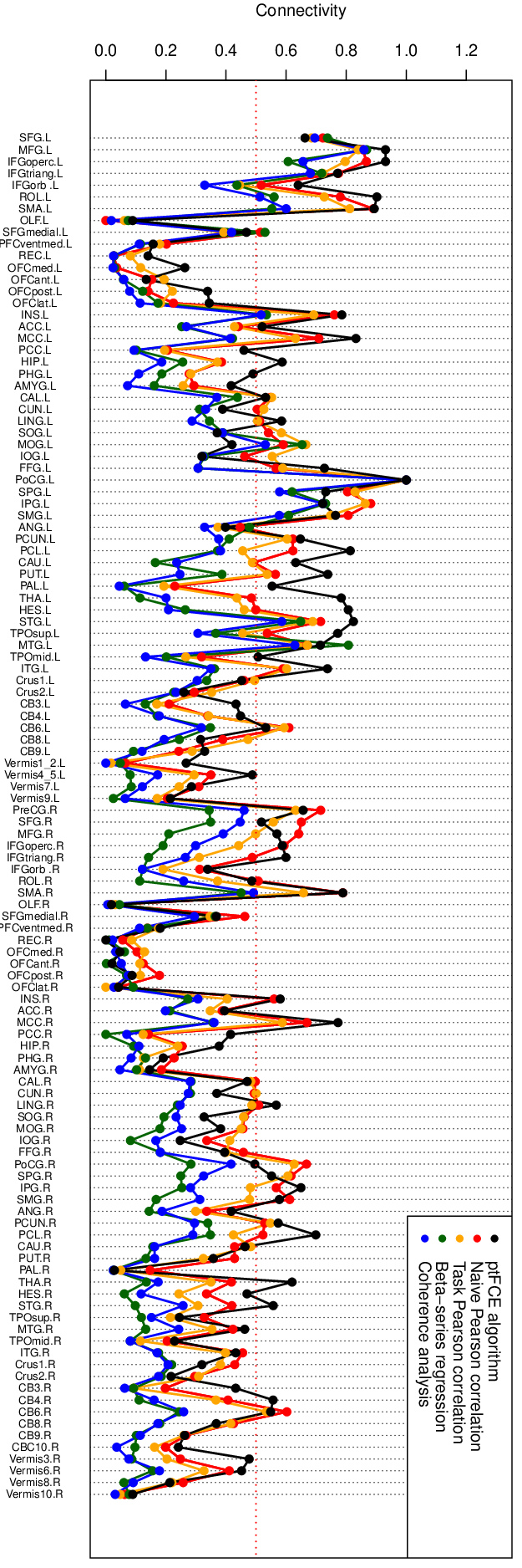
Refer to caption
Figure 5: Illustration of estimation results from five FC estimation methods. The horizontal axis indicates the 116116 regions compared to PreCG.L. The abbreviations of region names are provided in the data set aal2.120 in the R package brainGraph. The vertical axis presents the standardized connectivity measurements 𝒳r,j(s​t)\mathcal{X}_{r,j}^{(st)} between each region and the seed region PreCG.R. The red dotted horizontal line indicates the threshold 0.5 implemented for determining the connected/nonconnected relationships between PreCG.L and other regions.

Data Availability Statement

The data supporting the findings in Section 6 are publicly available on the HCP website:
https://protocols.humanconnectome.org/HCP/3T/task-fMRI-protocol-details.html (Barch et al. 2013).
The R code for simulation studies and data analyses is available at
https://github.com/KMengBrown/Population-level-Task-evoked-Functional-Connectivity.git.

Appendix — Supporting Materials for
“Population-level Task-evoked Functional Connectivity
via Fourier Analysis”

Appendix A Relationship between the proposed BOLD signal model and some existing models

In this paper, we implement the following model for observed task-fMRI BOLD signals Yk​(ω,t)Y_{k}(\omega;t), for ω∈Ω\omega\in\Omega and k∈{1,⋯,K}k\in\{1,\cdots,K\}.

(A.1) Yk​(ω,t)=Pk​(ω,t)+Qk​(ω,t)+ϵk​(ω,t),with\displaystyle Y_{k}(\omega;t)=P_{k}(\omega;t)+Q_{k}(\omega;t)+\epsilon_{k}(\omega;t),\ \ \mbox{with}
Pk​(ω,t)=βk​(ω)×N×hk​(t−t0,k),\displaystyle P_{k}(\omega;t)=\beta_{k}(\omega)\times N*h_{k}(t-t_{0,k}),

where Pk​(ω,t)P_{k}(\omega;t) denotes the BOLD signal component stemming solely from the task N⁡(t)N(t) of interest, Qk​(ω,t)Q_{k}(\omega;t) denotes spontaneous neural activity component and neural activity responding to nuisance tasks, and ϵk​(ω,t)\epsilon_{k}(\omega;t) is random error. Additionally, t0,kt_{0,k} denotes the population shared latency and is usually smaller than the experimental unit (e.g., see Zhang et al. 2013, p 138). The HRF shared by the whole population is hk​(t)h_{k}(t). Here, we explore three existing models for BOLD signals. We show that these models are special cases of our proposed BOLD signal model (A.1).

Example 1: Using the notations in our paper, the BOLD signal model implemented by Zhang et al. 2013 can be represented as follows.

(A.2) Yk​(ω,t)=Xk​(ω,t)T​d​(ω)+∑γ=1Γβk,γ​(ω)×(Nγ∗hk,γ)​(t)+ϵk​(ω,t),\displaystyle Y_{k}(\omega;t)=X_{k}(\omega;t)^{T}d(\omega)+\sum_{\gamma=1}^{\Gamma}\beta_{k,\gamma}(\omega)\times\left(N_{\gamma}*h_{k,\gamma}\right)(t)+\epsilon_{k}(\omega;t),

where Nγ​(t)N_{\gamma}(t) are task stimulus signals, hk,γ​(t)h_{k,\gamma}(t) are corresponding HRFs, and Xk​(ω,t)T​d​(ω)X_{k}(\omega;t)^{T}d(\omega) characterizes the BOLD signal components stemming from other known sources, e.g., respiration and heartbeat. The BOLD signal model proposed by Zhang et al. 2013 includes participant-dependent latency times. These latency times are essentially modeled as zero, since the values are usually much smaller than the corresponding experimental time unit.

Suppose we are interested in the first experimental task N1​(t)N_{1}(t). Define the following.

(A.3) βk​(ω):=βk,1​(ω),N⁡(t):=N1​(t),Pk​(ω,t)=βk​(ω)×(N∗hk)​(t),\displaystyle\beta_{k}(\omega):=\beta_{k,1}(\omega),\ \ N(t):=N_{1}(t),\ \ P_{k}(\omega;t)=\beta_{k}(\omega)\times\left(N*h_{k}\right)(t),
Qk​(ω,t):=Xk​(ω,t)T​d​(ω)+∑γ=2Γβk,γ​(ω)×(Nγ∗hk,γ)​(t).\displaystyle Q_{k}(\omega;t):=X_{k}(\omega;t)^{T}d(\omega)+\sum_{\gamma=2}^{\Gamma}\beta_{k,\gamma}(\omega)\times\left(N_{\gamma}*h_{k,\gamma}\right)(t).

Then (A.2) is equivalent to the model (A.1) with latency t0,k=0t_{0,k}=0, and there is no interaction term Pk​(ω,t)​Qk​(ω,t)P_{k}(\omega;t)Q_{k}(\omega;t).

Example 2: Using the notations in our paper, the BOLD signal model implemented by Warnick et al. 2018 is represented as follows (see Warnick et al. 2018, Equations (1) and (2)).

(A.4) Yk​(ω,t)=μk​(ω)+∑γ=1Γβk,γ​(ω)×(Nγ∗hk,γ)​(t)+ϵk​(ω,t),\displaystyle Y_{k}(\omega;t)=\mu_{k}(\omega)+\sum_{\gamma=1}^{\Gamma}\beta_{k,\gamma}(\omega)\times\left(N_{\gamma}*h_{k,\gamma}\right)(t)+\epsilon_{k}(\omega;t),

where Nγ​(t)N_{\gamma}(t) are task stimulus signals, hk,γ​(t)h_{k,\gamma}(t) are corresponding HRFs, ϵk​(ω,t)\epsilon_{k}(\omega;t) are random error, and μk​(ω)\mu_{k}(\omega) present the baseline. Suppose we are interested in task N1​(t)N_{1}(t). We apply the transform (A.3) and define Qk​(ω,t)=μk​(ω)+∑γ=2Γβk,γ​(ω)×(Nγ∗hk,γ)​(t)Q_{k}(\omega;t)=\mu_{k}(\omega)+\sum_{\gamma=2}^{\Gamma}\beta_{k,\gamma}(\omega)\times\left(N_{\gamma}*h_{k,\gamma}\right)(t). Then model (A.4) is equivalent to our proposed model (A.1) with latency t0,k=0t_{0,k}=0, without an interaction term Pk​(ω,t)​Qk​(ω,t)P_{k}(\omega;t)Q_{k}(\omega;t).

Example 3: Motivated by the independent component analysis framework, Joel et al. 2011 implemented the following model for task-fMRI BOLD signals.

Yk​(ω,t)=\displaystyle Y_{k}(\omega;t)= Mm,k​(ω)​{βt​m​(ω)×N×hk​(t)+βi​m​(ω)​ιm​(t)}\displaystyle M_{m,k}(\omega)\left\{\beta_{tm}(\omega)\times N*h_{k}(t)+\beta_{im}(\omega)\iota_{m}(t)\right\}
+Mv,k​(ω)​{βt​v​(ω)×N×hk​(t)+βi​v​(ω)​ιv​(t)}\displaystyle+M_{v,k}(\omega)\left\{\beta_{tv}(\omega)\times N*h_{k}(t)+\beta_{iv}(\omega)\iota_{v}(t)\right\}
(A.5) +Mb​(ω)​βb​(ω)​γ​(ω,t),\displaystyle+M_{b}(\omega)\beta_{b}(\omega)\gamma(\omega;t),

where M(⋅),kM_{(\cdot),k} is the spatial mask at the kt​hk^{th} node for visual cortex (Mv,kM_{v,k}), motor cortex (Mm,kM_{m,k}) or the whole brain (MbM_{b}), N⁡(t)N(t) is stimulus signal corresponding to the task of interest, hk​(t)h_{k}(t) is an HRF, ι(⋅)\iota_{(\cdot)} is the intrinsic activity of the corresponding cortex, γ⁡(ω,t)\gamma(\omega;t) presents random noise, and βt​m​(ω),βi​m​(ω),βt​v​(ω),βi​v​(ω),βb​(ω)\beta_{tm}(\omega),\beta_{im}(\omega),\beta_{tv}(\omega),\beta_{iv}(\omega),\beta_{b}(\omega) are the weights of motor task, intrinsic motor activity, visual task, intrinsic visual activity and noise, respectively.

Since the task of interest in the HCP data is a motor task, we define the following notations.

βk​(ω):=Mm,k​(ω)×βt​m​(ω),\displaystyle\beta_{k}(\omega):=M_{m,k}(\omega)\times\beta_{tm}(\omega),
Qk​(ω):=Mm,k​(ω)​βi​m​(ω)​ιm​(t)+Mv,k​(ω)​{βt​v​(ω)×N×hk​(t)+βi​v​(ω)​ιv​(t)},\displaystyle Q_{k}(\omega):=M_{m,k}(\omega)\beta_{im}(\omega)\iota_{m}(t)+M_{v,k}(\omega)\left\{\beta_{tv}(\omega)\times N*h_{k}(t)+\beta_{iv}(\omega)\iota_{v}(t)\right\},
ϵk​(ω,t)=Mb​(ω)​βb​(ω)​γ​(ω,t).\displaystyle\epsilon_{k}(\omega;t)=M_{b}(\omega)\beta_{b}(\omega)\gamma(\omega;t).

Using the notations above, model (A) is the same as model (A.1) with latency t0,k=0t_{0,k}=0, and there is no interaction term Pk​(ω,t)​Qk​(ω,t)P_{k}(\omega;t)Q_{k}(\omega;t).

Appendix B Lemmas, Theorems, and Their Proofs

In this section, we provide proofs of theorems and lemmas presented in our paper. Throughout this section, the time index collection 𝒯\mathcal{T} denotes {τ​Δ}τ=0T\{\tau\Delta\}_{\tau=0}^{T}, and Ω\Omega is a discrete and finite set.

Lemma B.1.

If f:𝒯→ℝf:\mathcal{T}\rightarrow\mathbb{R} is not constant zero, its Fourier transform f^​(ξ)\widehat{f}(\xi) has at most finitely many zero points (i.e., points ξ∈ℝ\xi\in\mathbb{R} such that f^​(ξ)=0\widehat{f}(\xi)=0) in any compact subset of ℝ\mathbb{R}.

Proof.

Define the complex function Φf​(z):=1T+1​∑τ=0Tf⁡(τ​Δ)​e−2​π​z​(τ​Δ)\Phi_{f}(z):=\frac{1}{T+1}\sum_{\tau=0}^{T}f(\tau\Delta)e^{-2\pi z(\tau\Delta)}, for all z=η+i​ξ∈ℂz=\eta+i\xi\in\mathbb{C}. Since it is straightforward that Φf​(z)\Phi_{f}(z) satisfies the Cauchy-Riemann equation ∂∂z¯​Φf​(z)=0\frac{\partial}{\partial\overline{z}}\Phi_{f}(z)=0, where ∂∂z¯=12​(∂∂η+i​∂∂ξ)\frac{\partial}{\partial\overline{z}}=\frac{1}{2}(\frac{\partial}{\partial\eta}+i\frac{\partial}{\partial\xi}) is a Wirtinger derivative, the Looman–Menchoff theorem implies that Φf​(z)\Phi_{f}(z) is a holomorphic function. Then the zero points of Φf​(z)\Phi_{f}(z) are isolated, i.e., every zero point has a neighbourhood that does not contain any other zero point (Conway 1973, Theorem 3.7). Therefore, f^​(ξ)=Φf​(i​ξ)\widehat{f}(\xi)=\Phi_{f}(i\xi) implies the desired result. □\square

Theorem B.1.

Suppose signals {Yk​(ω,t)|t∈𝒯}k=1K\{Y_{k}(\omega;t)|t\in\mathcal{T}\}_{k=1}^{K}, for ω∈Ω\omega\in\Omega, are defined as in (A.1), 𝔼​βk=𝔼​Rk​(t)=0\mathbb{E}\beta_{k}=\mathbb{E}R_{k}(t)=0, and t0,k=τ0,k​Δt_{0,k}=\tau_{0,k}\Delta with some τ0,k∈ℤ\tau_{0,k}\in\mathbb{Z} for all k=1,2,⋯,Kk=1,2,\cdots,K and t∈𝒯t\in\mathcal{T}. Let the random variable U:Ω→𝒯U:\Omega\rightarrow\mathcal{T} be uniformly distributed on 𝒯\mathcal{T}. Furthermore, we assume that U⁡(ω)U(\omega), {βk​(ω)}k=1K\{\beta_{k}(\omega)\}_{k=1}^{K}, and {Rk​(ω,t)|t∈𝒯}k=1K\{R_{k}(\omega;t)|t\in\mathcal{T}\}_{k=1}^{K} are independent. Then, the autocovariance differences 𝒜k​l​(s):=𝔼⁡{Yk​(t−U)​Yl​(t+s−U)}−𝔼⁡{Rk​(t−U)​Rl​(t+s−U)}\mathcal{A}_{kl}(s):=\mathbb{E}\left\{Y_{k}(t-U)Y_{l}(t+s-U)\right\}-\mathbb{E}\left\{R_{k}(t-U)R_{l}(t+s-U)\right\} depend only on ss, the Fourier transforms of 𝒜⁡(s)\mathcal{A}(s) are

𝒜^k​l​(ξ)=𝔼⁡(βk​βl)⋅|N^​(ξ)|2⋅h^k​(ξ)¯⋅h^l​(ξ)⋅e2​π​i​(t0,k−t0,l)​ξ.\displaystyle\widehat{\mathcal{A}}_{kl}(\xi)=\mathbb{E}\left(\beta_{k}\beta_{l}\right)\cdot\left|\widehat{N}(\xi)\right|^{2}\cdot\overline{\widehat{h}_{k}(\xi)}\,\cdot\,\widehat{h}_{l}(\xi)\,\cdot\,e^{2\pi i(t_{0,k}-t_{0,l})\xi}.

Furthermore, we have the following representation.

𝒞k​l​(ξ):=|𝒜^k​l​(ξ)|/|𝒜^k​k​(ξ)​𝒜^l​l​(ξ)|=|c​o​r​r​(βk,βl)|, for all ​ξ∈ℝ.\displaystyle\mathcal{C}_{kl}(\xi):=|\widehat{\mathcal{A}}_{kl}(\xi)|\Big/\sqrt{|\widehat{\mathcal{A}}_{kk}(\xi)\widehat{\mathcal{A}}_{ll}(\xi)|}=\left|corr\left(\beta_{k},\beta_{l}\right)\right|,\mbox{ for all }\xi\in\mathbb{R}.
Proof.

The independence between U⁡(ω)U(\omega), {βk​(ω)}k=1K\{\beta_{k}(\omega)\}_{k=1}^{K}, and {Rk​(ω,t)|t∈𝒯}k=1K\{R_{k}(\omega;t)|t\in\mathcal{T}\}_{k=1}^{K} implies

𝔼⁡[Yk​(t−U)​Yl​(t+s−U)]−𝔼⁡[Rk​(t−U)​Rl​(t+s−U)]\displaystyle\mathbb{E}[Y_{k}(t-U)Y_{l}(t+s-U)]-\mathbb{E}[R_{k}(t-U)R_{l}(t+s-U)]
=𝔼⁡(βk​βl)×𝔼⁡[(N∗hk)​(t−t0,k−U)×(N∗hl)​(t+s−t0,l−U)]\displaystyle=\mathbb{E}(\beta_{k}\beta_{l})\times\mathbb{E}\left[(N*h_{k})(t-t_{0,k}-U)\times(N*h_{l})(t+s-t_{0,l}-U)\right]
=𝔼(βkβl)×1T+1∑u=0T{(N∗hk)((τ−τ0,k−u)Δ)×(N∗hl)((s¯+τ0,k−τ0,l)Δ+(τ−τ0,k−u)Δ)}\displaystyle=\mathbb{E}(\beta_{k}\beta_{l})\times\frac{1}{T+1}\sum_{u=0}^{T}\Big\{(N*h_{k})\left((\tau-\tau_{0,k}-u)\Delta\right)\times(N*h_{l})\left((\underline{s}+\tau_{0,k}-\tau_{0,l})\Delta+(\tau-\tau_{0,k}-u)\Delta\right)\Big\}
=𝔼(βkβl)×1T+1∑v=−(τ−τ0,k)T−(τ−τ0,k){(N∗hk)(−vΔ)×(N∗hl)((s¯+τ0,k−τ0,l)Δ−vΔ)}\displaystyle=\mathbb{E}(\beta_{k}\beta_{l})\times\frac{1}{T+1}\sum_{v=-(\tau-\tau_{0,k})}^{T-(\tau-\tau_{0,k})}\Big\{(N*h_{k})\left(-v\Delta\right)\times(N*h_{l})\left((\underline{s}+\tau_{0,k}-\tau_{0,l})\Delta-v\Delta\right)\Big\}
(B.1) =𝔼(βkβl)×[N∗hk(−⋅)]∗[N∗hl](s+(t0,k−t0,l)),\displaystyle=\mathbb{E}(\beta_{k}\beta_{l})\times\left[N*h_{k}(-\cdot)\right]*\left[N*h_{l}\right]\left(s+(t_{0,k}-t_{0,l})\right),

which only depends on ss and does not depend on tt. Here, the last equality follows from the periodic extension and the definition of convolution. Then, we have the following Fourier transform,

𝒜^k​l​(ξ)\displaystyle\widehat{\mathcal{A}}_{kl}(\xi) =𝔼⁡(βk​βl)×(N∗hk)^​(ξ)¯​(N∗hl)^​(ξ)​e2​π​i​(t0,k−t0,l)​ξ\displaystyle=\mathbb{E}(\beta_{k}\beta_{l})\times\overline{\widehat{(N*h_{k})}(\xi)}\widehat{(N*h_{l})}(\xi)e^{2\pi i(t_{0,k}-t_{0,l})\xi}
=𝔼⁡(βk​βl)×|N^​(ξ)|2​hk^​(ξ)¯​hl^​(ξ)​e2​π​i​(t0,k−t0,l)​ξ,\displaystyle=\mathbb{E}(\beta_{k}\beta_{l})\times\left|\widehat{N}(\xi)\right|^{2}\overline{\widehat{h_{k}}(\xi)}\widehat{h_{l}}(\xi)e^{2\pi i(t_{0,k}-t_{0,l})\xi},

for all ξ∈ℝ\xi\in\mathbb{R}, which implies 𝒞k​l​(ξ)=|c​o​r​r​(βk,βl)|\mathcal{C}_{kl}(\xi)=\left|corr\left(\beta_{k},\beta_{l}\right)\right| for all ξ∈ℝ\xi\in\mathbb{R}. □\square

Lemma B.2.

The vector-valued stochastic process 𝐙⁡(ω,t)={(Z1​(ω,t),Z2​(ω,t),⋯,ZK​(ω,t))T}t∈𝒯\boldsymbol{Z}(\omega;t)=\{(Z_{1}(\omega;t),Z_{2}(\omega;t),\cdots,Z_{K}(\omega;t))^{T}\}_{t\in\mathcal{T}} is defined on probability space (Ω,2Ω,ℙ)(\Omega,2^{\Omega},\mathbb{P}) and is weakly stationary with mean zero, U:Ω→𝒯U:\Omega\rightarrow\mathcal{T} is uniformly distributed, and U⁡(ω)U(\omega) and 𝐙⁡(ω,t)\boldsymbol{Z}(\omega;t) are independent. Then the vector-valued stochastic process 𝐙⁡(ω,t−U⁡(ω))={(Z1​(ω,t−U⁡(ω)),Z2​(ω,t−U⁡(ω)),⋯,ZK​(ω,t−U⁡(ω)))T}t∈𝒯\boldsymbol{Z}(\omega;t-U(\omega))=\{(Z_{1}(\omega;t-U(\omega)),Z_{2}(\omega;t-U(\omega)),\cdots,Z_{K}(\omega;t-U(\omega)))^{T}\}_{t\in\mathcal{T}} is weakly stationary with mean zero as well. Additionally, 𝔼⁡[Zk​(t−U)​Zl​(t+s−U)]=𝔼⁡[Zk​(0)​Zl​(s)]\mathbb{E}[Z_{k}(t-U)Z_{l}(t+s-U)]=\mathbb{E}[Z_{k}(0)Z_{l}(s)], for all k,l=1,2,⋯,Kk,l=1,2,\cdots,K.

Proof.

Let μ\mu be the probability measure on 𝒯\mathcal{T} associated with the uniform random variable U:Ω→𝒯U:\Omega\rightarrow\mathcal{T}, i.e., μ=ℙ∘U−1\mu=\mathbb{P}\circ U^{-1}, then we have 𝔼⁡{Zk​(t−U)}=∫𝒯𝔼⁡{Zk​(t−U)|U=u}​μ​(𝑑u)\mathbb{E}\{Z_{k}(t-U)\}=\int_{\mathcal{T}}\mathbb{E}\{Z_{k}(t-U)|U=u\}\mu(du). The independence between UU and 𝒁\boldsymbol{Z} implies 𝔼⁡{Zk​(t−U)|U=u}=𝔼⁡{Zk​(t−u)}=0\mathbb{E}\{Z_{k}(t-U)|U=u\}=\mathbb{E}\{Z_{k}(t-u)\}=0 for all tt, which results in 𝔼⁡{Zk​(t−U)}=0\mathbb{E}\{Z_{k}(t-U)\}=0 for all t∈𝒯t\in\mathcal{T}. Similarly, we have

𝔼⁡{Zk​(t−U)​Zl​(t+s−U)}\displaystyle\mathbb{E}\left\{Z_{k}(t-U)Z_{l}(t+s-U)\right\} =∫𝒯𝔼⁡{Zk​(t−U)​Zl​(t+s−U)|U=u}​μ​(𝑑u)\displaystyle=\int_{\mathcal{T}}\mathbb{E}\left\{Z_{k}(t-U)Z_{l}(t+s-U)|U=u\right\}\mu(du)
=∫𝒯𝔼⁡{Zk​(t−u)​Zl​(t+s−u)}​μ​(𝑑u)\displaystyle=\int_{\mathcal{T}}\mathbb{E}\left\{Z_{k}(t-u)Z_{l}(t+s-u)\right\}\mu(du)
=∫𝒯𝔼⁡{Zk​(0)​Zl​(s)}​μ​(𝑑u)\displaystyle=\int_{\mathcal{T}}\mathbb{E}\left\{Z_{k}(0)Z_{l}(s)\right\}\mu(du)
=𝔼⁡{Zk​(0)​Zl​(s)},\displaystyle=\mathbb{E}\left\{Z_{k}(0)Z_{l}(s)\right\},

This completes the proof of the desired result. □\square

Theorem B.2.

Suppose we have the following random vectors and stochastic processes.

  • •

    𝔅:={(βk​(ω),βl​(ω))}ωn\mathfrak{B}:=\left\{(\beta_{k}(\omega),\beta_{l}(\omega))\right\}_{\omega}^{n} are nn i.i.d. random vectors.

  • •

    ℜ:={(R~k​(ω,t),R~l​(ω,t))|t∈𝒯}ω=1n\mathfrak{R}:=\left\{\left(\tilde{R}_{k}(\omega;t),\tilde{R}_{l}(\omega;t)\right)|t\in\mathcal{T}\right\}_{\omega=1}^{n} are nn i.i.d. stochastic processes.

  • •

    𝔚:={(Wk​(ω,t),Wl​(ω,t))|t∈𝒯}ω=1n\mathfrak{W}:=\left\{\left(W_{k}(\omega;t),W_{l}(\omega;t)\right)|t\in\mathcal{T}\right\}_{\omega=1}^{n} are nn i.i.d. stochastic processes satisfying (i) random vectors (Wk​(ω,t1),Wl​(ω,t1))\left(W_{k}(\omega;t_{1}),W_{l}(\omega;t_{1})\right) and (Wk​(ω,t2),Wl​(ω,t2))\left(W_{k}(\omega;t_{2}),W_{l}(\omega;t_{2})\right) are independent whenever t1≠t2t_{1}\neq t_{2}, (ii) the stochastic process {(Wk​(ω,t),Wl​(ω,t))|t∈𝒯}\{\left(W_{k}(\omega;t),W_{l}(\omega;t)\right)|t\in\mathcal{T}\} is weakly stationary with mean zero, and (iii) Σk​l=𝔼⁡{Wk​(t)​Wl​(t)}\Sigma_{kl}=\mathbb{E}\left\{W_{k}(t)W_{l}(t)\right\} for all t∈𝒯t\in\mathcal{T}.

The collections 𝔅,ℜ,𝔚\mathfrak{B},\mathfrak{R},\mathfrak{W} are independent. Furthermore, we have the following task-fMRI BOLD signals.† 22 2 †\dagger: Observed task-fMRI BOLD signals are Yk​(ω,t)=βk​(ω)×N×hk​(t−t0,k)+Rk​(ω,t)Y_{k}(\omega;t)=\beta_{k}(\omega)\times N*h_{k}(t-t_{0,k})+R_{k}(\omega;t), where Rk​(ω,t)R_{k}(\omega;t) are true reference signals. However, the true reference signals are not observable in applications and should be estimated by R~k​(ω,t)\tilde{R}_{k}(\omega;t) using the AMUSE algorithm. The corresponding estimation bias Rk​(ω,t)−R~k​(ω,t)R_{k}(\omega;t)-\tilde{R}_{k}(\omega;t) is denoted by Wk​(ω,t)W_{k}(\omega;t). Hence, we have Yk​(ω,t)=βk​(ω)×N×hk​(t−t0,k)+R~k​(ω,t)+Wk​(ω,t)Y_{k}(\omega;t)=\beta_{k}(\omega)\times N*h_{k}(t-t_{0,k})+\tilde{R}_{k}(\omega;t)+W_{k}(\omega;t), which is just a representation of Yk​(ω,t)=βk​(ω)×N×hk​(t−t0,k)+Rk​(ω,t)Y_{k}(\omega;t)=\beta_{k}(\omega)\times N*h_{k}(t-t_{0,k})+R_{k}(\omega;t).

Yk′​(ω,t)=βk′​(ω)×N×hk′​(t−t0,k′)+R~k′​(ω,t)+Wk′​(ω,t),\displaystyle Y_{k^{\prime}}(\omega;t)=\beta_{k^{\prime}}(\omega)\times N*h_{k^{\prime}}(t-t_{0,{k^{\prime}}})+\tilde{R}_{k^{\prime}}(\omega;t)+W_{k^{\prime}}(\omega;t),

for k′∈{k,l}k^{\prime}\in\{k,l\} and ω=1,⋯,n\omega=1,\cdots,n. We define the following estimator for 𝒞k​l​(ξ)\mathcal{C}_{kl}(\xi).

𝒞k​le​s​t,n​(ξ):=|𝒜k​le​s​t,n^​(ξ)|/|𝒜k​ke​s​t,n^​(ξ)​𝒜l​le​s​t,n^​(ξ)|,for all ​ξ∈ℝ,\displaystyle\mathcal{C}_{kl}^{est,n}(\xi):=\left|\widehat{\mathcal{A}_{kl}^{est,n}}(\xi)\right|\Bigg/\sqrt{\left|\widehat{\mathcal{A}_{kk}^{est,n}}(\xi)\widehat{\mathcal{A}_{ll}^{est,n}}(\xi)\right|},\ \ \ \mbox{for all }\xi\in\mathbb{R},

where hat (⋅)^\widehat{(\cdot)} denotes the Fourier transform and

𝒜k​le​s​t,n​(s):=\displaystyle\mathcal{A}_{kl}^{est,n}(s):= 1T+1​∑t∈{τ​Δ}τ=0T[1n​∑ω=1n{Yk​(ω,t−U⁡(ω))​Yl​(ω,t+s−U⁡(ω))}]\displaystyle\frac{1}{T+1}\sum_{t\in\{\tau\Delta\}_{\tau=0}^{T}}\left[\frac{1}{n}\sum_{\omega=1}^{n}\left\{Y_{k}\left(\omega;t-U(\omega)\right)Y_{l}(\omega;t+s-U(\omega))\right\}\right]
−1T+1∑t∈{τ​Δ}τ=0T[1n∑ω=1n{R~k(ω;t−U(ω))R~l(ω;t+s−U(ω))}].\displaystyle-\frac{1}{T+1}\sum_{t\in\{\tau\Delta\}_{\tau=0}^{T}}\left[\frac{1}{n}\sum_{\omega=1}^{n}\left\{\tilde{R}_{k}(\omega;t-U(\omega))\tilde{R}_{l}(\omega;t+s-U(\omega))\right\}\right].

Then we have the following asymptotic behavior of 𝒞k​le​s​t,n​(ξ)\mathcal{C}_{kl}^{est,n}(\xi) as n→∞n\rightarrow\infty.

(B.2) ℙ{limn→∞𝒞k​le​s​t,n(ξ)=|𝔼⁡(βk​βl)​h^k​(ξ)¯​h^l​(ξ)|h^k​(ξ)​h^l​(ξ)|​e2​π​i​ξ​(t0,k−t0,l)+Σk​l(T+1)​|N^​(ξ)|2​|h^k​(ξ)​h^l​(ξ)||(𝔼⁡(βk2)+Σk​k(T+1)​|N^​(ξ)​h^k​(ξ)|2)​(𝔼⁡(βl2)+Σl​l(T+1)​|N^​(ξ)​h^l​(ξ)|2)}=1.\displaystyle\mathbb{P}\left\{\lim_{n\rightarrow\infty}\mathcal{C}^{est,n}_{kl}(\xi)=\frac{\left|\mathbb{E}(\beta_{k}\beta_{l})\frac{\overline{\widehat{h}_{k}(\xi)}\widehat{h}_{l}(\xi)}{\left|\widehat{h}_{k}(\xi)\widehat{h}_{l}(\xi)\right|}e^{2\pi i\xi(t_{0,k}-t_{0,l})}+\frac{\Sigma_{kl}}{(T+1)\left|\widehat{N}(\xi)\right|^{2}\left|\widehat{h}_{k}(\xi)\widehat{h}_{l}(\xi)\right|}\right|}{\sqrt{\left(\mathbb{E}(\beta_{k}^{2})+\frac{\Sigma_{kk}}{(T+1)\left|\widehat{N}(\xi)\widehat{h}_{k}(\xi)\right|^{2}}\right)\left(\mathbb{E}(\beta_{l}^{2})+\frac{\Sigma_{ll}}{(T+1)\left|\widehat{N}(\xi)\widehat{h}_{l}(\xi)\right|^{2}}\right)}}\right\}=1.
Proof.

For each pair (s,t)∈𝒯2(s,t)\in\mathcal{T}^{2}, the strong law of large numbers implies that there exists 𝒩s,t∈2Ω\mathcal{N}_{s,t}\in 2^{\Omega} depending on the pair (s,t)(s,t) such that ℙ⁡(𝒩s,t)=0\mathbb{P}(\mathcal{N}_{s,t})=0 and

1n​∑ω=1n[{Yk​(ω,t−U⁡(ω))​Yl​(ω,t+s−U⁡(ω))}−{R~k​(ω,t−U⁡(ω))​R~l​(ω,t+s−U⁡(ω))}]\displaystyle\frac{1}{n}\sum_{\omega=1}^{n}\left[\left\{Y_{k}\left(\omega;t-U(\omega)\right)Y_{l}(\omega;t+s-U(\omega))\right\}-\left\{\tilde{R}_{k}\left(\omega;t-U(\omega)\right)\tilde{R}_{l}(\omega;t+s-U(\omega))\right\}\right]
→𝔼⁡{Yk​(t−U)​Yl​(t+s−U)}−𝔼⁡{R~k​(t−U)​R~l​(t+s−U)}=:𝒟k​l​(t,s),\displaystyle\rightarrow\mathbb{E}\left\{Y_{k}(t-U)Y_{l}(t+s-U)\right\}-\mathbb{E}\left\{\tilde{R}_{k}(t-U)\tilde{R}_{l}(t+s-U)\right\}=:\mathcal{D}_{kl}(t,s),

in Ω−𝒩s,t\Omega-\mathcal{N}_{s,t} as n→∞n\rightarrow\infty. Then we have

(B.3) limn→∞𝒜k​le​s​t,n​(s)=1T+1​∑t∈{τ​Δ}τ=0T𝒟k​l​(t,s)\displaystyle\lim_{n\rightarrow\infty}\mathcal{A}_{kl}^{est,n}(s)=\frac{1}{T+1}\sum_{t\in\{\tau\Delta\}_{\tau=0}^{T}}\mathcal{D}_{kl}(t,s)

for all s∈𝒯s\in\mathcal{T} in Ω−𝒩\Omega-\mathcal{N}, where 𝒩:=⋃s,t∈𝒯𝒩s,t\mathcal{N}:=\bigcup_{{s,t}\in\mathcal{T}}\mathcal{N}_{s,t}. The limit (B.3) implies the following in Ω−𝒩\Omega-\mathcal{N}.

limn→∞𝒜k​le​s​t,n^​(ξ)\displaystyle\lim_{n\rightarrow\infty}\widehat{\mathcal{A}_{kl}^{est,n}}(\xi) =limn→∞{1T+1​∑s∈{τ​Δ}τ=0T𝒜k​le​s​t,n​(s)​e2​π​i​ξ​s}\displaystyle=\lim_{n\rightarrow\infty}\left\{\frac{1}{T+1}\sum_{s\in\{\tau\Delta\}_{\tau=0}^{T}}\mathcal{A}_{kl}^{est,n}(s)e^{2\pi i\xi s}\right\}
=1T+1​∑s∈{τ​Δ}τ=0Tlimn→∞{𝒜k​le​s​t,n​(s)}​e2​π​i​ξ​s\displaystyle=\frac{1}{T+1}\sum_{s\in\{\tau\Delta\}_{\tau=0}^{T}}\lim_{n\rightarrow\infty}\left\{\mathcal{A}_{kl}^{est,n}(s)\right\}e^{2\pi i\xi s}
=1T+1​∑t∈{τ​Δ}τ=0T{1T+1​∑s∈{τ​Δ}τ=0T𝒟k​l​(t,s)​e2​π​i​ξ​s}\displaystyle=\frac{1}{T+1}\sum_{t\in\{\tau\Delta\}_{\tau=0}^{T}}\left\{\frac{1}{T+1}\sum_{s\in\{\tau\Delta\}_{\tau=0}^{T}}\mathcal{D}_{kl}(t,s)e^{2\pi i\xi s}\right\}

for all ξ∈ℝ\xi\in\mathbb{R}. In the derivation above, we change the order of summation and limit as the summation contains only finitely many terms. Since 1T+1​∑s∈{τ​Δ}τ=0T𝒟k​l​(t,s)​e2​π​i​ξ​s\frac{1}{T+1}\sum_{s\in\{\tau\Delta\}_{\tau=0}^{T}}\mathcal{D}_{kl}(t,s)e^{2\pi i\xi s} is the Fourier transform of 𝒟k​l​(t,s)\mathcal{D}_{kl}(t,s) with respect to ss, repeating the calculation strategy in (B), we have

1T+1​∑s∈{τ​Δ}τ=0T𝒟k​l​(t,s)​e2​π​i​ξ​s=𝔼⁡(βk​βl)​h^k​(ξ)¯​h^l​(ξ)|h^k​(ξ)​h^l​(ξ)|​e2​π​i​ξ​(t0,k−t0,l)+Σk​l(T+1)​|N^​(ξ)|2​|h^k​(ξ)​h^l​(ξ)|,\displaystyle\frac{1}{T+1}\sum_{s\in\{\tau\Delta\}_{\tau=0}^{T}}\mathcal{D}_{kl}(t,s)e^{2\pi i\xi s}=\mathbb{E}(\beta_{k}\beta_{l})\frac{\overline{\widehat{h}_{k}(\xi)}\widehat{h}_{l}(\xi)}{\left|\widehat{h}_{k}(\xi)\widehat{h}_{l}(\xi)\right|}e^{2\pi i\xi(t_{0,k}-t_{0,l})}+\frac{\Sigma_{kl}}{(T+1)\left|\widehat{N}(\xi)\right|^{2}\left|\widehat{h}_{k}(\xi)\widehat{h}_{l}(\xi)\right|},

which does not depend on tt. Then we have

(B.4) limn→∞𝒜k​le​s​t,n^​(ξ)=𝔼⁡(βk​βl)​h^k​(ξ)¯​h^l​(ξ)|h^k​(ξ)​h^l​(ξ)|​e2​π​i​ξ​(t0,k−t0,l)+Σk​l(T+1)​|N^​(ξ)|2​|h^k​(ξ)​h^l​(ξ)|\displaystyle\lim_{n\rightarrow\infty}\widehat{\mathcal{A}_{kl}^{est,n}}(\xi)=\mathbb{E}(\beta_{k}\beta_{l})\frac{\overline{\widehat{h}_{k}(\xi)}\widehat{h}_{l}(\xi)}{\left|\widehat{h}_{k}(\xi)\widehat{h}_{l}(\xi)\right|}e^{2\pi i\xi(t_{0,k}-t_{0,l})}+\frac{\Sigma_{kl}}{(T+1)\left|\widehat{N}(\xi)\right|^{2}\left|\widehat{h}_{k}(\xi)\widehat{h}_{l}(\xi)\right|}

for all ξ∈ℝ\xi\in\mathbb{R} in Ω−𝒩\Omega-\mathcal{N}. The limit (B.4) implies

limn→∞𝒞k​le​s​t,n​(ξ)\displaystyle\lim_{n\rightarrow\infty}\mathcal{C}_{kl}^{est,n}(\xi) =|limn→∞𝒜k​le​s​t,n^​(ξ)|/|limn→∞𝒜k​ke​s​t,n^​(ξ)×limn→∞𝒜l​le​s​t,n^​(ξ)|\displaystyle=\left|\lim_{n\rightarrow\infty}\widehat{\mathcal{A}_{kl}^{est,n}}(\xi)\right|\Bigg/\sqrt{\left|\lim_{n\rightarrow\infty}\widehat{\mathcal{A}_{kk}^{est,n}}(\xi)\times\lim_{n\rightarrow\infty}\widehat{\mathcal{A}_{ll}^{est,n}}(\xi)\right|}
=|𝔼⁡(βk​βl)​h^k​(ξ)¯​h^l​(ξ)|h^k​(ξ)​h^l​(ξ)|​e2​π​i​ξ​(t0,k−t0,l)+Σk​l(T+1)​|N^​(ξ)|2​|h^k​(ξ)​h^l​(ξ)||(𝔼⁡(βk2)+Σk​k(T+1)​|N^​(ξ)​h^k​(ξ)|2)​(𝔼⁡(βl2)+Σl​l(T+1)​|N^​(ξ)​h^l​(ξ)|2)\displaystyle=\frac{\left|\mathbb{E}(\beta_{k}\beta_{l})\frac{\overline{\widehat{h}_{k}(\xi)}\widehat{h}_{l}(\xi)}{\left|\widehat{h}_{k}(\xi)\widehat{h}_{l}(\xi)\right|}e^{2\pi i\xi(t_{0,k}-t_{0,l})}+\frac{\Sigma_{kl}}{(T+1)\left|\widehat{N}(\xi)\right|^{2}\left|\widehat{h}_{k}(\xi)\widehat{h}_{l}(\xi)\right|}\right|}{\sqrt{\left(\mathbb{E}(\beta_{k}^{2})+\frac{\Sigma_{kk}}{(T+1)\left|\widehat{N}(\xi)\widehat{h}_{k}(\xi)\right|^{2}}\right)\left(\mathbb{E}(\beta_{l}^{2})+\frac{\Sigma_{ll}}{(T+1)\left|\widehat{N}(\xi)\widehat{h}_{l}(\xi)\right|^{2}}\right)}}

for all ξ∈ℝ\xi\in\mathbb{R} in Ω−𝒩\Omega-\mathcal{N}. Since ℙ⁡(𝒩)=ℙ⁡(⋃s,t∈𝒯𝒩s,t)≤∑s,t∈𝒯ℙ⁡(𝒩s,t)=0\mathbb{P}(\mathcal{N})=\mathbb{P}\left(\bigcup_{s,t\in\mathcal{T}}\mathcal{N}_{s,t}\right)\leq\sum_{s,t\in\mathcal{T}}\mathbb{P}(\mathcal{N}_{s,t})=0, the desired result (B.2) follows. □\square

Proof of Theorem 4.1 in the manuscript: Since {ϵ⁡(ω,t)}t∈𝒯\{\epsilon(\omega;t)\}_{t\in\mathcal{T}} is WSMZ, Lemma B.2 implies that {ϵ⁡(ω,t−U⁡(ω))}t∈𝒯\{\epsilon(\omega;t-U(\omega))\}_{t\in\mathcal{T}} is WSMZ as well. Because of 𝔼⁡[βk,γ]=0\mathbb{E}[\beta_{k,\gamma}]=0 and the independence between βk,γ​(ω)\beta_{k,\gamma}(\omega) and U⁡(ω)U(\omega), we have 𝔼⁡[Rk​(t−U)]=0\mathbb{E}[R_{k}(t-U)]=0 for all tt. Additionally, the independence assumption in Theorem 4.1 implies the following

𝔼⁡[Rk​(t−U)⋅Rk​(t+s−U)]=𝔼⁡[Qk​(t−U)⋅Qk​(t+s−U)]+𝔼⁡[ϵk​(t−U)⋅ϵk​(t+s−U)]\displaystyle\mathbb{E}[R_{k}(t-U)\cdot R_{k}(t+s-U)]=\mathbb{E}[Q_{k}(t-U)\cdot Q_{k}(t+s-U)]+\mathbb{E}[\epsilon_{k}(t-U)\cdot\epsilon_{k}(t+s-U)]

Proof of Theorem 4.2 in the manuscript: In the following equation provided in Theorem 4.1, 𝑷\boldsymbol{P} is a permutation matrix and 𝚲\boldsymbol{\Lambda} is a diagonal matrix.

(B.5) (111β∗0)=𝑨​𝚲−1​𝑷−1.\displaystyle\begin{pmatrix}1&1\\ \frac{1}{\beta^{*}}&0\end{pmatrix}=\boldsymbol{A}\boldsymbol{\Lambda}^{-1}\boldsymbol{P}^{-1}.

Then equation (B.5) implies β∗=βk​(ω)=a1​i′/a2​i′\beta^{*}=\beta_{k}(\omega)=a_{1i^{\prime}}/a_{2i^{\prime}} for some i′∈{1,2}i^{\prime}\in\{1,2\} and a2​j=0a_{2j}=0 when j≠i′j\neq i^{\prime}. Furthermore, the pair (𝑨,𝑺⁡(ω,t))(\boldsymbol{A},\boldsymbol{S}(\omega;t)) also satisfies the following equation, which is provided in Theorem 4.1 as well.

(B.6) 𝑨​(s1​(ω,t)s2​(ω,t))=(111β∗0)​(Jk​(ω,t)Rk​(ω,t−U⁡(ω)))=(Yk​(ω,t−U⁡(ω))−β∗​Ck(N∗hk)​(t−t0,k−U⁡(ω))−Ck),\displaystyle\boldsymbol{A}\begin{pmatrix}s_{1}(\omega;t)\\ s_{2}(\omega;t)\end{pmatrix}=\begin{pmatrix}1&1\\ \frac{1}{\beta^{*}}&0\end{pmatrix}\begin{pmatrix}J_{k}(\omega;t)\\ R_{k}(\omega;t-U(\omega))\end{pmatrix}=\begin{pmatrix}Y_{k}(\omega;t-U(\omega))-\beta^{*}C_{k}\\ (N*h_{k})(t-t_{0,k}-U(\omega))-C_{k}\end{pmatrix},

and equation (B.6) implies a2​i′​si′​(ω,t)=(N∗hk)​(t−t0,k−U⁡(ω))−Cka_{2i^{\prime}}s_{i^{\prime}}(\omega;t)=(N*h_{k})(t-t_{0,k}-U(\omega))-C_{k}. Therefore, we have

a1​i′​si′​(ω,t)=a1​i′a2​i′×a2​i′​si′​(ω,t)=βk​(ω)×{(N∗hk)​(t−t0,k−U⁡(ω))−Ck}=Jk​(ω,t).\displaystyle a_{1i^{\prime}}s_{i^{\prime}}(\omega;t)=\frac{a_{1i^{\prime}}}{a_{2i^{\prime}}}\times a_{2i^{\prime}}s_{i^{\prime}}(\omega;t)=\beta_{k}(\omega)\times\left\{(N*h_{k})(t-t_{0,k}-U(\omega))-C_{k}\right\}=J_{k}(\omega;t).

The following theorem supports our Assumption 2.

Theorem B.3.

Let signals {Qk​(ω,t)}t∈𝒯\{Q_{k}(\omega;t)\}_{t\in\mathcal{T}} be of the following form

(B.7) Qk​(ω,t)={∑γ=1Γβk,γ​(ω)×N~γ×h~k,γ​(t)}.\displaystyle Q_{k}(\omega;t)=\left\{\sum_{\gamma=1}^{\Gamma}\beta_{k,\gamma}(\omega)\times\tilde{N}_{\gamma}*\tilde{h}_{k,\gamma}(t)\right\}.

Let {ϵk​(ω,t)}t∈𝒯\{\epsilon_{k}(\omega;t)\}_{t\in\mathcal{T}} be a random error signal. U⁡(ω)U(\omega) is a random variable uniformly distributed on 𝒯\mathcal{T}. Suppose the following conditions are satisfied:

  1. i)

    𝔼​βk,γ=0\mathbb{E}\beta_{k,\gamma}=0 for all γ=1,…,Γ\gamma=1,\ldots,\Gamma;

  2. ii)

    U⁡(ω)U(\omega), βk,1​(ω)\beta_{k,1}(\omega), βk,2​(ω),…,βk,Γ​(ω)\beta_{k,2}(\omega),\ldots,\beta_{k,\Gamma}(\omega), and {ϵk​(ω,t)}t∈𝒯\{\epsilon_{k}(\omega;t)\}_{t\in\mathcal{T}} are independent;

  3. iii)

    {ϵk​(ω,t)}t∈𝒯\{\epsilon_{k}(\omega;t)\}_{t\in\mathcal{T}} is WSMZ.

Then, the reference term {Rk(ω;t)=Qk(ω;t)+ϵk(ω;t)}t∈𝒯\{R_{k}(\omega;t)=Q_{k}(\omega;t)+\epsilon_{k}(\omega;t)\}_{t\in\mathcal{T}} is WSMZ.

Remark: If the condition i) is not satisfied, we may apply the following centralization

Rk​(ω,t)−ℝ⁡[Rk​(t)]={∑γ=1Γ[βk,γ​(ω)−𝔼⁡(βk,γ)]×N~γ×h~k,γ​(t)}+(ϵk​(ω,t)−𝔼⁡[ϵk​(t)])\displaystyle R_{k}(\omega;t)-\mathbb{R}[R_{k}(t)]=\left\{\sum_{\gamma=1}^{\Gamma}\left[\beta_{k,\gamma}(\omega)-\mathbb{E}(\beta_{k,\gamma})\right]\times\tilde{N}_{\gamma}*\tilde{h}_{k,\gamma}(t)\right\}+\left(\epsilon_{k}(\omega;t)-\mathbb{E}[\epsilon_{k}(t)]\right)

and use [βk,γ​(ω)−𝔼⁡(βk,γ)]\left[\beta_{k,\gamma}(\omega)-\mathbb{E}(\beta_{k,\gamma})\right] as βk,γ​(ω)\beta_{k,\gamma}(\omega).

Proof.

The conditions i) and ii) imply

𝔼⁡[Rk​(t−U)]={∑γ=1Γ𝔼​βk,γ×𝔼⁡[N~γ∗h~k,γ​(t−U)]}+𝔼⁡[ϵk​(t−U)]=𝔼⁡[ϵk​(t−U)].\displaystyle\mathbb{E}[R_{k}(t-U)]=\left\{\sum_{\gamma=1}^{\Gamma}\mathbb{E}\beta_{k,\gamma}\times\mathbb{E}\left[\tilde{N}_{\gamma}*\tilde{h}_{k,\gamma}(t-U)\right]\right\}+\mathbb{E}[\epsilon_{k}(t-U)]=\mathbb{E}[\epsilon_{k}(t-U)].

In addition, the condition iii), together with Lemma B.2, implies that {ϵk​(ω,t−U⁡(ω))}t∈𝒯\{\epsilon_{k}(\omega;t-U(\omega))\}_{t\in\mathcal{T}} is WSMZ, hence,

𝔼⁡[Rk​(t−U)]=𝔼⁡[ϵk​(t−U)]=0.\displaystyle\mathbb{E}[R_{k}(t-U)]=\mathbb{E}[\epsilon_{k}(t-U)]=0.

Condition ii) implies the following

𝔼⁡[Rk​(t−U)⋅Rk​(t+s−U)]=𝔼⁡[Qk​(t−U)⋅Qk​(t+s−U)]+𝔼⁡[ϵk​(t−U)⋅ϵk​(t+s−U)].\displaystyle\mathbb{E}[R_{k}(t-U)\cdot R_{k}(t+s-U)]=\mathbb{E}[Q_{k}(t-U)\cdot Q_{k}(t+s-U)]+\mathbb{E}[\epsilon_{k}(t-U)\cdot\epsilon_{k}(t+s-U)].

Since {ϵk​(ω,t−U⁡(ω))}t∈𝒯\{\epsilon_{k}(\omega;t-U(\omega))\}_{t\in\mathcal{T}} is WSMZ, the second term above depends only on ss. The condition ii) implies the following

𝔼⁡[Qk​(t−U)⋅Qk​(t+s−U)]={∑γ=1Γ𝔼⁡(βk,γ2)×𝔼⁡[N~γ∗h~k,γ​(t−U)⋅N~γ∗h~k,γ​(t+s−U)]}.\displaystyle\mathbb{E}[Q_{k}(t-U)\cdot Q_{k}(t+s-U)]=\left\{\sum_{\gamma=1}^{\Gamma}\mathbb{E}\left(\beta_{k,\gamma}^{2}\right)\times\mathbb{E}\left[\tilde{N}_{\gamma}*\tilde{h}_{k,\gamma}(t-U)\cdot\tilde{N}_{\gamma}*\tilde{h}_{k,\gamma}(t+s-U)\right]\right\}.

The calculation in Eq. (B) indicates that 𝔼⁡[N~γ∗h~k,γ​(t−U)⋅N~γ∗h~k,γ​(t+s−U)]\mathbb{E}\left[\tilde{N}_{\gamma}*\tilde{h}_{k,\gamma}(t-U)\cdot\tilde{N}_{\gamma}*\tilde{h}_{k,\gamma}(t+s-U)\right] depends only on ss. Hence, 𝔼⁡[Qk​(t−U)⋅Qk​(t+s−U)]\mathbb{E}[Q_{k}(t-U)\cdot Q_{k}(t+s-U)] depends only on ss. Therefore, the reference term {Rk(ω;t)=Qk(ω;t)+ϵk(ω;t)}t∈𝒯\{R_{k}(\omega;t)=Q_{k}(\omega;t)+\epsilon_{k}(\omega;t)\}_{t\in\mathcal{T}} is WSMZ. □\square

Appendix C Identifiability of Task-evoked Terms

In this section, we prove the identifiability of task-evoked terms using the identifiability theory proposed by Tong et al. 1991. To implement this theory, we need a uniformly distributed random variable UU as an auxiliary variable. In our approach to estimating ptFC, the auxiliary random variable UU is artificially generated. Hence, all the distributional information of UU, e.g., its independence, is viewed as available.

We generate U:Ω→𝒯U:\Omega\rightarrow\mathcal{T} to be a uniformly distributed random variable. Identifying the task-evoked terms Pk​(ω,t)P_{k}(\omega;t) from Yk​(ω,t)=Pk​(ω,t)+Rk​(ω,t)Y_{k}(\omega;t)=P_{k}(\omega;t)+R_{k}(\omega;t) is equivalent to identifying Pk​(ω,t−U⁡(ω))P_{k}(\omega;t-U(\omega)) from Yk​(ω,t−U⁡(ω))Y_{k}(\omega;t-U(\omega)). Specifically, the identification of the task-evoked terms Pk​(ω,t)P_{k}(\omega;t) consists of the following steps:

  1. i)

    We first generate random variable U⁡(ω)U(\omega);

  2. ii)

    then, we identify Pk​(ω,t−U⁡(ω))P_{k}(\omega;t-U(\omega)) from Yk​(ω,t−U⁡(ω))=Pk​(ω,t−U⁡(ω))+Rk​(ω,t−U⁡(ω))Y_{k}(\omega;t-U(\omega))=P_{k}(\omega;t-U(\omega))+R_{k}(\omega;t-U(\omega));

  3. iii)

    lastly, we identify Pk​(ω,t)P_{k}(\omega;t) by taking the transform Pk​(ω,t−U⁡(ω))↦Pk​(ω,t)P_{k}(\omega;t-U(\omega))\mapsto P_{k}(\omega;t).

To prove the identifiability of the task-evoked terms Pk​(ω,t)P_{k}(\omega;t), it suffices to show the identifiability in the second step above. Our proposed BOLD signal model Yk​(ω,t−U⁡(ω))=Pk​(ω,t−U⁡(ω))+Rk​(ω,t−U⁡(ω))Y_{k}(\omega;t-U(\omega))=P_{k}(\omega;t-U(\omega))+R_{k}(\omega;t-U(\omega)) can be represented in the following “mixing” form.

(C.1) Yk​(ω,t−U⁡(ω))=(1001)​(Pk​(ω,t−U⁡(ω))Rk​(ω,t−U⁡(ω))),\displaystyle Y_{k}\left(\omega;t-U(\omega)\right)=\begin{pmatrix}1&0\\ 0&1\end{pmatrix}\begin{pmatrix}P_{k}(\omega;t-U(\omega))\\ R_{k}(\omega;t-U(\omega))\end{pmatrix},

where the identity matrix mixes the source signals Pk​(ω,t−U⁡(ω))P_{k}(\omega;t-U(\omega)) and Rk​(ω,t−U⁡(ω))R_{k}(\omega;t-U(\omega)).

In this section, we provide the identifiability of the task-evoked terms Pk​(ω,t−U⁡(ω))=βk​(ω)​N∗hk​(t−t0,k−U⁡(ω))P_{k}(\omega;t-U(\omega))=\beta_{k}(\omega)N*h_{k}(t-t_{0,k}-U(\omega)) as well as reference terms Rk​(ω,t−U⁡(ω))R_{k}(\omega;t-U(\omega)) in (C.1), up to deterministic coefficients, among the family of mixing forms defined as follows.

(C.2) ℳ:={(s1​(ω,t)s2​(ω,t))|∃𝑨∈ℝ2×2​ such that ​Yk​(ω,t−U⁡(ω))=𝑨​(s1​(ω,t)s2​(ω,t))},\displaystyle\mathcal{M}:=\left\{\begin{pmatrix}s_{1}(\omega;t)\\ s_{2}(\omega;t)\end{pmatrix}\,\Bigg|\,\exists\boldsymbol{A}\in\mathbb{R}^{2\times 2}\mbox{ such that }Y_{k}\left(\omega;t-U(\omega)\right)=\boldsymbol{A}\begin{pmatrix}s_{1}(\omega;t)\\ s_{2}(\omega;t)\end{pmatrix}\right\},

where all matrices 𝑨\boldsymbol{A} are deterministic 2-by-2 matrices mixing source signals s1​(ω,t)s_{1}(\omega;t) and s2​(ω,t)s_{2}(\omega;t). Specifically, we will show that, under some probabilistic conditions, all the stochastic signals (s1​(ω,t),s2​(ω,t))\left(s_{1}(\omega;t),s_{2}(\omega;t)\right) in (C.2) are proportional to (Pk​(ω,t−U⁡(ω)),Rk​(ω,t−U⁡(ω)))(P_{k}(\omega;t-U(\omega)),R_{k}(\omega;t-U(\omega))) or (Rk​(ω,t−U⁡(ω)),Pk​(ω,t−U⁡(ω)))(R_{k}(\omega;t-U(\omega)),P_{k}(\omega;t-U(\omega))). Then the task-evoked terms Pk​(ω,t−U⁡(ω))P_{k}(\omega;t-U(\omega)) are identifiable in ℳ\mathcal{M} in the following sense: there exist i′∈{1,2}i^{\prime}\in\{1,2\} and λ≠0\lambda\neq 0 such that si′​(ω,t)=λ​Pk​(ω,t−U⁡(ω))={λ​βk​(ω)}​N∗hk​(t−t0,k−U⁡(ω))s_{i^{\prime}}(\omega;t)=\lambda P_{k}(\omega;t-U(\omega))=\{\lambda\beta_{k}(\omega)\}N*h_{k}(t-t_{0,k}-U(\omega)) for all t∈𝒯t\in\mathcal{T}. Since the deterministic coefficient λ\lambda is canceled out in computing c​o​r​r​(βk,βl)corr(\beta_{k},\beta_{l}), the identifiability of Pk​(ω,t)P_{k}(\omega;t) up to a deterministic coefficient implies the exact identifiability of ptFC |c​o​r​r​(βk,βl)||corr(\beta_{k},\beta_{l})|.

The following theorem implies the identifiability of Pk​(ω,t)P_{k}(\omega;t) and provides a formal foundation for the discussion above.

Theorem C.1.

Let U:Ω→𝒯U:\Omega\rightarrow\mathcal{T} be uniformly distributed. Suppose U⁡(ω)U(\omega), βk​(ω)\beta_{k}(\omega), and {Rk​(ω,t)|t∈𝒯}\{R_{k}(\omega;t)|t\in\mathcal{T}\} are independent, and {Rk​(ω,t−U⁡(ω))}t∈𝒯\{R_{k}(\omega;t-U(\omega))\}_{t\in\mathcal{T}} is WSMZ. Furthermore, we assume that there exists a t∗∈𝒯t^{*}\in\mathcal{T} such that

𝔼⁡{Pk​(t−U)​Pk​(t−t∗−U)}𝔼​{Pk​(t−U)}2≠𝔼⁡{Rk​(t−U)​Rk​(t−t∗−U)}𝔼​{Rk​(t−U)}2.\displaystyle\frac{\mathbb{E}\left\{P_{k}(t-U)P_{k}(t-t^{*}-U)\right\}}{\mathbb{E}\left\{P_{k}(t-U)\right\}^{2}}\neq\frac{\mathbb{E}\left\{R_{k}(t-U)R_{k}(t-t^{*}-U)\right\}}{\mathbb{E}\left\{R_{k}(t-U)\right\}^{2}}.

If there exists a WSMZ stochastic process (s1​(ω,t),s2​(ω,t))(s_{1}(\omega;t),s_{2}(\omega;t)) such that {s1​(ω,t)}t∈𝒯\{s_{1}(\omega;t)\}_{t\in\mathcal{T}} and {s2​(ω,t)}t∈𝒯\{s_{2}(\omega;t)\}_{t\in\mathcal{T}} are uncorrelated,

𝔼⁡{s1​(t)​s1​(t−t∗)}𝔼​{s1​(t)}2≠𝔼⁡{s2​(t)​s2​(t−t∗)}𝔼​{s2​(t)}2, and\displaystyle\frac{\mathbb{E}\left\{s_{1}(t)s_{1}(t-t^{*})\right\}}{\mathbb{E}\left\{s_{1}(t)\right\}^{2}}\neq\frac{\mathbb{E}\left\{s_{2}(t)s_{2}(t-t^{*})\right\}}{\mathbb{E}\left\{s_{2}(t)\right\}^{2}},\mbox{ and}
Yk​(ω,t−U⁡(ω))=Pk​(ω,t−U⁡(ω))+Rk​(ω,t−U⁡(ω))=𝑨​(s1​(ω,t)s2​(ω,t))\displaystyle Y_{k}(\omega;t-U(\omega))=P_{k}(\omega;t-U(\omega))+R_{k}(\omega;t-U(\omega))=\boldsymbol{A}\begin{pmatrix}s_{1}(\omega;t)\\ s_{2}(\omega;t)\end{pmatrix}

for some deterministic 2-by-2 matrix 𝐀\boldsymbol{A}, then there exists a permutation matrix 𝐏\boldsymbol{P} and a non-singular diagonal matrix 𝚲\boldsymbol{\Lambda} such that

(C.3) (Pk​(ω,t−U⁡(ω))Rk​(ω,t−U⁡(ω)))=𝑷​𝚲​(s1​(ω,t)s2​(ω,t)).\displaystyle\begin{pmatrix}P_{k}(\omega;t-U(\omega))\\ R_{k}(\omega;t-U(\omega))\end{pmatrix}=\boldsymbol{P\Lambda}\begin{pmatrix}s_{1}(\omega;t)\\ s_{2}(\omega;t)\end{pmatrix}.

Remark: (i) Our discussion of identifiability presented at the beginning of this section is based on (C.3). (ii) Since 𝔼​βk=𝔼​Rk​(t)=0\mathbb{E}\beta_{k}=\mathbb{E}R_{k}(t)=0 for all tt, we have 𝔼⁡{Pk​(t1)​Rk​(t2)}=0\mathbb{E}\left\{P_{k}(t_{1})R_{k}(t_{2})\right\}=0 for all t1,t2∈𝒯t_{1},t_{2}\in\mathcal{T}, i.e., Pk​(ω,t1)P_{k}(\omega;t_{1}) and Rk​(ω,t2)R_{k}(\omega;t_{2}) are uncorrelated. (iii) One can verify that Pk​(ω,t−U⁡(ω))=βk​(ω)​N∗hk​(t−t0,k−U⁡(ω))P_{k}(\omega;t-U(\omega))=\beta_{k}(\omega)N*h_{k}(t-t_{0,k}-U(\omega)) is WSMZ.

Based on these remarks, Theorem C.1 is a straightforward result following from Theorem 2 of Tong et al. 1991.

Appendix D Bias and Variance — Performance of ptFCE in Estimating ptFCs

In this section, we analyze the performance of the ptFCE algorithm in terms of estimation bias and variance from both theoretical and simulational perspectives.

We first provide the estimation bias mechanism of the ptFCE algorithm motivated by

(D.1) ℙ{limn→∞𝒞k​le​s​t,n(ξ)=|𝔼⁡(βk​βl)​h^k​(ξ)¯​h^l​(ξ)|h^k​(ξ)​h^l​(ξ)|​e2​π​i​ξ​(t0,k−t0,l)+Σk​l(T+1)​|N^​(ξ)|2​|h^k​(ξ)​h^l​(ξ)||(𝔼⁡(βk2)+Σk​k(T+1)​|N^​(ξ)​h^k​(ξ)|2)​(𝔼⁡(βl2)+Σl​l(T+1)​|N^​(ξ)​h^l​(ξ)|2)}=1,\displaystyle\mathbb{P}\left\{\lim_{n\rightarrow\infty}\mathcal{C}^{est,n}_{kl}(\xi)=\frac{\left|\mathbb{E}(\beta_{k}\beta_{l})\frac{\overline{\widehat{h}_{k}(\xi)}\widehat{h}_{l}(\xi)}{\left|\widehat{h}_{k}(\xi)\widehat{h}_{l}(\xi)\right|}e^{2\pi i\xi(t_{0,k}-t_{0,l})}+\frac{\Sigma_{kl}}{(T+1)\left|\widehat{N}(\xi)\right|^{2}\left|\widehat{h}_{k}(\xi)\widehat{h}_{l}(\xi)\right|}\right|}{\sqrt{\left(\mathbb{E}(\beta_{k}^{2})+\frac{\Sigma_{kk}}{(T+1)\left|\widehat{N}(\xi)\widehat{h}_{k}(\xi)\right|^{2}}\right)\left(\mathbb{E}(\beta_{l}^{2})+\frac{\Sigma_{ll}}{(T+1)\left|\widehat{N}(\xi)\widehat{h}_{l}(\xi)\right|^{2}}\right)}}\right\}=1,

which is from Supplementary Theorem B.2. Because the quantities in

Σk​k/[(T+1)​|N^​(ξ)​h^k​(ξ)|2]≈0,Σl​l/[(T+1)​|N^​(ξ)​h^l​(ξ)|2]≈0.\displaystyle\Sigma_{kk}\Big/[(T+1)|\widehat{N}(\xi)\widehat{h}_{k}(\xi)|^{2}]\approx 0,\ \ \ \Sigma_{ll}\Big/[(T+1)|\widehat{N}(\xi)\widehat{h}_{l}(\xi)|^{2}]\approx 0.

are not exactly zeros, the asymptotic estimation bias

|limn→∞𝒞k​le​s​t,n​(ξ)−𝒞k​l​(ξ)|=|limn→∞𝒞k​le​s​t,n​(ξ)−|𝔼⁡(βk​βl)|𝔼⁡(βk2)​𝔼​(βl2)|\displaystyle\left|\lim_{n\rightarrow\infty}\mathcal{C}^{est,n}_{kl}(\xi)-\mathcal{C}_{kl}(\xi)\right|=\left|\lim_{n\rightarrow\infty}\mathcal{C}^{est,n}_{kl}(\xi)-\frac{\left|\mathbb{E}(\beta_{k}\beta_{l})\right|}{\sqrt{\mathbb{E}(\beta_{k}^{2})\mathbb{E}(\beta_{l}^{2})}}\right|

always exists. We further model that approximation residual Wk′​(ω,t)=Rk′​(ω,t)−R~k′​(ω,t)W_{k^{\prime}}(\omega;t)=R_{k^{\prime}}(\omega;t)-\tilde{R}_{k^{\prime}}(\omega;t) at different nodes are independent, implying Σk​l=0\Sigma_{kl}=0 in (D.1). Then the following inequality, as a result of (D.1), indicates that our ptFCE algorithm tends to underestimate ptFC.

limn→∞𝒞k​le​s​t,n​(ξ)\displaystyle\lim_{n\rightarrow\infty}\mathcal{C}_{kl}^{est,n}(\xi) =a.s.|𝔼⁡(βk​βl)|(𝔼⁡(βk2)+Σk​k(T+1)​|N^​(ξ)​h^k​(ξ)|2)​(𝔼⁡(βl2)+Σl​l(T+1)​|N^​(ξ)​h^l​(ξ)|2)\displaystyle=_{a.s.}\frac{\left|\mathbb{E}(\beta_{k}\beta_{l})\right|}{\sqrt{\left(\mathbb{E}(\beta_{k}^{2})+\frac{\Sigma_{kk}}{(T+1)\left|\widehat{N}(\xi)\widehat{h}_{k}(\xi)\right|^{2}}\right)\left(\mathbb{E}(\beta_{l}^{2})+\frac{\Sigma_{ll}}{(T+1)\left|\widehat{N}(\xi)\widehat{h}_{l}(\xi)\right|^{2}}\right)}}
(D.2) ≤|𝔼⁡(βk​βl)|𝔼⁡(βk2)​𝔼​(βl2)=|c​o​r​r​(βk,βl)|.\displaystyle\leq\frac{\left|\mathbb{E}(\beta_{k}\beta_{l})\right|}{\sqrt{\mathbb{E}(\beta_{k}^{2})\mathbb{E}(\beta_{l}^{2})}}=|corr(\beta_{k},\beta_{l})|.

Furthermore, the larger the variance of the noise ϵk​(ω,t)\epsilon_{k}(\omega;t) in

Yk(ω;t)=βk(ω)×(N∗hk)(t−t0,k)+Rk(ω;t),t∈𝒯,k=1,⋯,K,ω∈Ω,\displaystyle Y_{k}(\omega;t)=\beta_{k}(\omega)\times\left(N*h_{k}\right)\left(t-t_{0,k}\right)+R_{k}(\omega;t),\ \ t\in\mathcal{T},\ \ k=1,\cdots,K,\ \ \omega\in\Omega,

the less accurate is the approximation Rk′​(ω,t)≈R~k′​(ω,t)R_{k^{\prime}}(\omega;t)\approx\tilde{R}_{k^{\prime}}(\omega;t) and the larger Σk​k\Sigma_{kk} and Σl​l\Sigma_{ll} in the inequality (D). Hence, the larger the variance of noise ϵk​(ω,t)\epsilon_{k}(\omega;t), the larger the underestimation bias. The formula above also indicates that the larger the underlying ptFC, the larger the underestimation bias. Subsequent simulations confirm all the conclusions on bias presented herein. We also show that the underestimation bias is moderate in general in terms of estimating ptFCs.

We present the performance of ptFCE in estimating ptFC by investigating estimation bias and variance using simulated data. Specifically, suppose the true ptFC in our simulation mechanism is ρ\rho, and the estimated ptFC from this algorithm is ρ^\widehat{\rho}, then we investigate bias ρ^−ρ\widehat{\rho}-\rho and the variance of ρ^\widehat{\rho}. We implement the following data-generating mechanism, compatible with the definition of ptFC. The main steps of this mechanism are the following, while the details are provided in Appendix E.

Mechanism 0: Step 1, we generate random coefficients (β1​(ω),β2​(ω))T∼N2​(𝟎,(σi​j)1≤i,j≤2)\left(\beta_{1}(\omega),\beta_{2}(\omega)\right)^{T}\sim N_{2}\left(\boldsymbol{0},(\sigma_{ij})_{1\leq i,j\leq 2}\right) for ω=1,⋯,n\omega=1,\cdots,n, and ρ:=|σ12/σ11​σ22|\rho:=|\sigma_{12}/\sqrt{\sigma_{11}\sigma_{22}}| is the true underlying ptFC between synthetic nodes 11 and 22. Step 2, we generate reference signals {Rk′(ω;τΔ)=Qk′(ω;τΔ)+ϵk′(ω;τΔ)}τ=0T\{R_{k^{\prime}}(\omega;\tau\Delta)=Q_{k^{\prime}}(\omega;\tau\Delta)+\epsilon_{k^{\prime}}(\omega;\tau\Delta)\}_{\tau=0}^{T} for ω=1,⋯,n\omega=1,\cdots,n and k′∈{1,2}k^{\prime}\in\{1,2\}, where the 2​n​T2nT noise values {ϵk′(ω;τΔ)|k′=1,2;ω=1,⋯,n;τ=0,⋯,T}∼i​i​dN(0,V)\{\epsilon_{k^{\prime}}(\omega;\tau\Delta)|k^{\prime}=1,2;\omega=1,\cdots,n;\tau=0,\cdots,T\}\sim_{iid}N(0,V). Step 3, we compute the signals {Yk′(ω;τΔ)|k′=1,2}τ=0T\{Y_{k^{\prime}}(\omega;\tau\Delta)|k^{\prime}=1,2\}_{\tau=0}^{T}, for ω=1,⋯,n\omega=1,\cdots,n, by Yk′​(ω,τ​Δ)=9000+βk′​(ω)×(N∗hk′)​(τ​Δ)+Rk′​(ω,τ​Δ)Y_{k^{\prime}}(\omega;\tau\Delta)=9000+\beta_{k^{\prime}}(\omega)\times\left(N*h_{k^{\prime}}\right)(\tau\Delta)+R_{k^{\prime}}(\omega;\tau\Delta).

We investigate sample sizes n∈{50,100,308,1000}n\in\{50,100,308,1000\}, where 308308 is the sample size of the HCP dataset used to obtain the results in our paper. We apply the ptFCE algorithm to estimate the underlying ρ\rho from synthetic signals. The corresponding estimate is denoted by ρ^\widehat{\rho}. For each ρ∈{0.25,0.5,0.75}\rho\in\{0.25,0.5,0.75\}, we repeat this procedure 500 times. The resulting estimates ρ^\hat{\rho} are summarized in Supplementary Table 3 and Supplementary Figure 6.

Table 3: The summaries of the estimated ρ^\widehat{\rho} in different underlying ptFC ρ\rho scenarios. The percentage in the parenthesis after each mean shows the corresponding relative bias (ρ^−ρ)/ρ(\widehat{\rho}-\rho)/\rho, where the minus signs indicate underestimation.
ρ=0.25\rho=0.25 ρ=0.5\rho=0.5 ρ=0.75\rho=0.75
mean sd mean sd mean sd
n=50n=50 0.255 (2%\%) 0.120 0.456 (-8.8%\%) 0.114 0.670 (-10.7%\%) 0.081
n=100n=100 0.246 (-1.6%\%) 0.093 0.460 (-8%\%) 0.079 0.671 (-10.5%\%) 0.055
n=308n=308 0.248 (-0.8%\%) 0.055 0.457 (-8.6%\%) 0.047 0.670 (-10.7%\%) 0.030
n=1000n=1000 0.246 (-1.6%\%) 0.028 0.462 (-7.6%\%) 0.026 0.675 (-10%\%) 0.018
Refer to caption
Figure 6: The boxplots summarizing the estimated ρ^\widehat{\rho} in different underlying ptFC ρ\rho and different sample sizes nn scenarios.

In addition, we provide a simulation study for different signal-to-noise ratios. Specifically, we investigate the influence of random noise {ϵk′(ω;τΔ)}k′,τ,ω∼i​i​dN(0,V)\{\epsilon_{k^{\prime}}(\omega;\tau\Delta)\}_{k^{\prime},\tau,\omega}\sim_{iid}N(0,V) on the ptFCE algorithm. Specifically, we fix sample size n=308n=308; for each λ∈[0.5,5]\lambda\in[0.5,5], we conduct the 500-run simulation study described above except we change the random noise to {ϵk′(ω;τΔ)}k′,τ,ω∼i​i​dN(0,λV)\{\epsilon_{k^{\prime}}(\omega;\tau\Delta)\}_{k^{\prime},\tau,\omega}\sim_{iid}N(0,\lambda V). For each λ\lambda and simulation run rr, the estimated ptFC between synthetic nodes is denoted as ρ^λ(r)\widehat{\rho}_{\lambda}^{(r)}, then we obtain 500 curves {ρ^λ(r)|λ∈[0.5,5]}r=1500\{\widehat{\rho}_{\lambda}^{(r)}|\lambda\in[0.5,5]\}_{r=1}^{500} presented in Supplementary Figure 7.

Refer to caption
Figure 7: The red, orange, and green curves present the collections {ρ^λ(r)|λ∈[0.5,5]}r=1500\{\widehat{\rho}_{\lambda}^{(r)}|\lambda\in[0.5,5]\}_{r=1}^{500} corresponding to underlying ptFC ρ=0.25,0.5,0.75\rho=0.25,0.5,0.75. The three blue solid curves present the mean curves {1500​∑r=1500ρ^λ(r)|λ∈[0.5,5]}\{\frac{1}{500}\sum_{r=1}^{500}\widehat{\rho}_{\lambda}^{(r)}|\lambda\in[0.5,5]\} in the three underlying ptFC scenarios, and the three black dotted lines present the three underlying ptFC.

As expected from the theoretical analysis of the bias mechanism, our proposed ptFCE algorithm tends to underestimate true ptFCs, see Supplementary Table 3 and Supplementary Figures 6 and 7. But Supplementary Table 3 shows that the bias is moderate. Simulations also confirm other conclusions on estimation bias presented in the theoretical analysis above. Additionally, Supplementary Figure 3 shows that the magnitude of noise ϵk​(ω,t)\epsilon_{k}(\omega;t) does not influence the variance of the ptFCE estimates. The increase in sample size reduces estimation variance.

Appendix E Data-generating Mechanisms for Simulations

In this section, we provide the details of Mechanisms 0, 1, and 2 for generating synthetic signals in simulation studies in our paper. To mimic the HCP data of interest, we apply the following parameters in the two data-generating mechanisms.

  • •

    Repeatition time Δ=0.72\Delta=0.72 (seconds)

  • •

    Number of observation time points T=283T=283.

  • •

    The task of interest (squeezing right toes) is presented by the stimulus signal N(t)=𝟏[86.5,98.5)(t)+𝟏[162,174)(t)N(t)=\mathbf{1}_{[86.5,98.5)}(t)+\mathbf{1}_{[162,174)}(t).

  • •

    The tasks that are not of interest are presented by stimulus signals N~1(t)=𝟏[71.35,83.35)(t)+𝟏[177.125,189.125)(t)\tilde{N}_{1}(t)=\mathbf{1}_{[71.35,83.35)}(t)+\mathbf{1}_{[177.125,189.125)}(t), N~2(t)=𝟏[11,23)(t)+𝟏[116.63,128.63)(t)\tilde{N}_{2}(t)=\mathbf{1}_{[11,23)}(t)+\mathbf{1}_{[116.63,128.63)}(t), N~3(t)=𝟏[26.13,38.13)(t)+𝟏[146.88,158.88)(t)\tilde{N}_{3}(t)=\mathbf{1}_{[26.13,38.13)}(t)+\mathbf{1}_{[146.88,158.88)}(t), and N~4(t)=𝟏[56.26,68.26)(t)+𝟏[131.75,143.75)(t)\tilde{N}_{4}(t)=\mathbf{1}_{[56.26,68.26)}(t)+\mathbf{1}_{[131.75,143.75)}(t). They correspond to the tasks of squeezing left toes, squeezing left/right fingers, and moving tongue.

  • •

    HRF functions hkh_{k} and h~k,γ\tilde{h}_{k,\gamma}, for k∈{1,3}k\in\{1,3\} and γ∈{1,2,3,4}\gamma\in\{1,2,3,4\}, are the double-gamma variate functions implemented in the R function canonicalHRF with parameters a1=4=4, a2=10=10, b1=0.8=0.8, b2=0.8=0.8, c=0.4=0.4; HRF functions h2h_{2} and h~2,γ\tilde{h}_{2,\gamma}, for γ∈{1,2,3,4}\gamma\in\{1,2,3,4\}, are the same function with parameters a1=8=8, a2=14=14, b1=1=1, b2=1=1, c=0.3=0.3. It is important to emphasize that none of the HRFs herein is canonical. The curves of all HRF functions used in our simulations studies are presented in Supplementary Figure 8.

Refer to caption
Figure 8: The black solid curve presents the canonical HRF (the R function canonicalHRF with default parameters). The blue dashed curve presents the R function canonicalHRF with parameters a1=4=4, a2=10=10, b1=0.8=0.8, b2=0.8=0.8, c=0.4=0.4. The red dotted curve presents the R function canonicalHRF with parameters a1=8=8, a2=14=14, b1=1=1, b2=1=1, c=0.3=0.3.

E.1 Mechanism 0

This mechanism is based on the task-fMRI BOLD signal model proposed in our paper. Specifically, we implement the following model to generate synthetic data.

(E.1) Yk′​(ω,t)=9000+βk′×N×hk′​(t)+{∑γ=14βk′,γ​(ω)×N~γ×h~k′,γ​(t)}+ϵk′​(ω,t),\displaystyle Y_{k^{\prime}}(\omega;t)=9000+\beta_{k^{\prime}}\times N*h_{k^{\prime}}(t)+\left\{\sum_{\gamma=1}^{4}\beta_{k^{\prime},\gamma}(\omega)\times\tilde{N}_{\gamma}*\tilde{h}_{k^{\prime},\gamma}(t)\right\}+\epsilon_{k^{\prime}}(\omega;t),
where ​t∈𝒯={τ​Δ}τ=0T​ and ​k′∈{1,2}.\displaystyle\mbox{where }t\in\mathcal{T}=\{\tau\Delta\}_{\tau=0}^{T}\mbox{ and }k^{\prime}\in\{1,2\}.

We generate signals {(Y1(ω;τΔ),Y2(ω;τΔ)}τ=0T\{(Y_{1}(\omega;\tau\Delta),Y_{2}(\omega;\tau\Delta)\}_{\tau=0}^{T}, for ω=1,⋯,n\omega=1,\cdots,n, by the following steps.

  • •

    Step 1: Generate bivariate normal random vectors (β1(ω),β2(ω))T∼i.i.d.N2((0,0)T,(σi​j)1≤i,j≤2)\left(\beta_{1}(\omega),\beta_{2}(\omega)\right)^{T}\sim_{i.i.d.}N_{2}\left((0,0)^{T},(\sigma_{ij})_{1\leq i,j\leq 2}\right) for ω=1,⋯,n\omega=1,\cdots,n, where ρ:=|σ12/σ11​σ22|\rho:=|\sigma_{12}/\sqrt{\sigma_{11}\sigma_{22}}| is the true underlying ptFC, and

    (E.2) σ11=2,σ22=3,σ12=ρ×σ11​σ22.\displaystyle\sigma_{11}=2,\ \ \sigma_{22}=3,\ \ \sigma_{12}=\rho\times\sqrt{\sigma_{11}\sigma_{22}}.
  • •

    Step 2: For each γ∈{1,2,3,4}\gamma\in\{1,2,3,4\}, generate bivariate normal random vector

    (β1,γ​(ω)β2,γ​(ω))∼i.i.d.N2((00),(20.3×2×30.3×2×33)),\displaystyle\begin{pmatrix}\beta_{1,\gamma}(\omega)\\ \beta_{2,\gamma}(\omega)\end{pmatrix}\sim_{i.i.d.}N_{2}\left(\begin{pmatrix}0\\ 0\end{pmatrix},\begin{pmatrix}2&0.3\times\sqrt{2\times 3}\\ 0.3\times\sqrt{2\times 3}&3\end{pmatrix}\right),

    for ω=1,⋯,n\omega=1,\cdots,n. The four collections {(β1,γ​(ω),β2,γ​(ω))T}ω=1n\left\{\left(\beta_{1,\gamma}(\omega),\beta_{2,\gamma}(\omega)\right)^{T}\right\}_{\omega=1}^{n}, for γ∈{1,2,3,4}\gamma\in\{1,2,3,4\}, are independently generated.

  • •

    Step 3: For each fixed ω∈{1,⋯,n}\omega\in\{1,\cdots,n\}, generate (white) noise as follows.

    (ϵ1​(ω,τ​Δ)ϵ2​(ω,τ​Δ))∼i.i.d.N2((00),(300030)), for τ=0,⋯,T.\displaystyle\begin{pmatrix}\epsilon_{1}(\omega;\tau\Delta)\\ \epsilon_{2}(\omega;\tau\Delta)\end{pmatrix}\sim_{i.i.d.}N_{2}\left(\begin{pmatrix}0\\ 0\end{pmatrix},\begin{pmatrix}30&0\\ 0&30\end{pmatrix}\right),\mbox{ for }\tau=0,\cdots,T.

    The nn collections {(ϵ1​(ω,τ​Δ),ϵ2​(ω,τ​Δ))}τ=0T\left\{\left(\epsilon_{1}(\omega;\tau\Delta),\epsilon_{2}(\omega;\tau\Delta)\right)\right\}_{\tau=0}^{T}, for ω∈{1,⋯,n}\omega\in\{1,\cdots,n\}, are independently generated.

  • •

    Step 4: Compute the signals {(Y1(ω;τΔ),Y2(ω;τΔ)}τ=0T\{(Y_{1}(\omega;\tau\Delta),Y_{2}(\omega;\tau\Delta)\}_{\tau=0}^{T}, for ω=1,⋯,n\omega=1,\cdots,n, by model (E.1).

A pair of simulated {(Y1(ω;τΔ),Y2(ω;τΔ)}τ=0T\{(Y_{1}(\omega;\tau\Delta),Y_{2}(\omega;\tau\Delta)\}_{\tau=0}^{T} using Mechanisms 0 is presented in Supplementary Figure 9.

Refer to caption
Figure 9: Left panels present signals generated for node 1, and right panels present signals generated for node 2. The underlying ptFCs for pairs in the upper, middle, and lower rows are 0.25, 0.5, and 0.75, respectively.

E.2 Mechanism 1

Mechanism 1 is very similar to Mechanism 0 and is based on (E.1) as well, except for k′∈{1,2,3}k^{\prime}\in\{1,2,3\}. We generate signals {(Y1(ω;τΔ),Y2(ω;τΔ),Y3(ω;τΔ)}τ=0T\{(Y_{1}(\omega;\tau\Delta),Y_{2}(\omega;\tau\Delta),Y_{3}(\omega;\tau\Delta)\}_{\tau=0}^{T}, for ω=1,⋯,n\omega=1,\cdots,n, using the following steps.

  • •

    Step 1: Generate normal random vectors (β1(ω),β2(ω),β3(ω))T∼i.i.d.N3(𝟎,(σi​j)1≤i,j≤3)\left(\beta_{1}(\omega),\beta_{2}(\omega),\beta_{3}(\omega)\right)^{T}\sim_{i.i.d.}N_{3}\left(\boldsymbol{0},(\sigma_{ij})_{1\leq i,j\leq 3}\right) for ω=1,⋯,n\omega=1,\cdots,n, where

    (E.3) (σi​j)1≤i,j≤3=(2ρ12×2×30ρ12×2×33ρ23×2×30ρ23×2×32),\displaystyle\left(\sigma_{ij}\right)_{1\leq i,j\leq 3}=\begin{pmatrix}2&\rho_{12}\times\sqrt{2\times 3}&0\\ \rho_{12}\times\sqrt{2\times 3}&3&\rho_{23}\times\sqrt{2\times 3}\\ 0&\rho_{23}\times\sqrt{2\times 3}&2\end{pmatrix},

    and ρi​j:=|σi​j/σi​i​σj​j|\rho_{ij}:=|\sigma_{ij}/\sqrt{\sigma_{ii}\sigma_{jj}}| for (i,j)∈{(1,2),(2,3)}(i,j)\in\{(1,2),(2,3)\} are the true underlying ptFCs.

  • •

    Step 2: For each γ∈{1,2,3,4}\gamma\in\{1,2,3,4\}, generate bivariate normal random vector

    (β1,γ​(ω)β2,γ​(ω)β3,γ​(ω))∼i.i.d.N3((000),(20.3×2×300.3×2×330.3×2×300.3×2×32)),\displaystyle\begin{pmatrix}\beta_{1,\gamma}(\omega)\\ \beta_{2,\gamma}(\omega)\\ \beta_{3,\gamma}(\omega)\end{pmatrix}\sim_{i.i.d.}N_{3}\left(\begin{pmatrix}0\\ 0\\ 0\end{pmatrix},\begin{pmatrix}2&0.3\times\sqrt{2\times 3}&0\\ 0.3\times\sqrt{2\times 3}&3&0.3\times\sqrt{2\times 3}\\ 0&0.3\times\sqrt{2\times 3}&2\end{pmatrix}\right),

    for ω=1,⋯,n\omega=1,\cdots,n. The four collections {(β1,γ​(ω),β2,γ​(ω),β3,γ​(ω))}ω=1n\left\{\left(\beta_{1,\gamma}(\omega),\beta_{2,\gamma}(\omega),\beta_{3,\gamma}(\omega)\right)\right\}_{\omega=1}^{n}, for γ∈{1,2,3,4}\gamma\in\{1,2,3,4\}, are independently generated.

  • •

    Step 3: For each fixed ω∈{1,⋯,n}\omega\in\{1,\cdots,n\}, generate (white) noise as follows.

    (ϵ1​(ω,τ​Δ)ϵ2​(ω,τ​Δ)ϵ3​(ω,τ​Δ))∼i.i.d.N3((000),(300003000030)), for τ=0,⋯,T.\displaystyle\begin{pmatrix}\epsilon_{1}(\omega;\tau\Delta)\\ \epsilon_{2}(\omega;\tau\Delta)\\ \epsilon_{3}(\omega;\tau\Delta)\end{pmatrix}\sim_{i.i.d.}N_{3}\left(\begin{pmatrix}0\\ 0\\ 0\end{pmatrix},\begin{pmatrix}30&0&0\\ 0&30&0\\ 0&0&30\end{pmatrix}\right),\mbox{ for }\tau=0,\cdots,T.

    The nn collections {(ϵ1​(ω,τ​Δ),ϵ2​(ω,τ​Δ),ϵ3​(ω,τ​Δ))}τ=0T\left\{\left(\epsilon_{1}(\omega;\tau\Delta),\epsilon_{2}(\omega;\tau\Delta),\epsilon_{3}(\omega;\tau\Delta)\right)\right\}_{\tau=0}^{T}, for ω∈{1,⋯,n}\omega\in\{1,\cdots,n\}, are independently generated.

  • •

    Step 4: Compute the signals {(Y1(ω;τΔ),Y2(ω;τΔ),Y3(ω;τΔ)}τ=0T\{(Y_{1}(\omega;\tau\Delta),Y_{2}(\omega;\tau\Delta),Y_{3}(\omega;\tau\Delta)\}_{\tau=0}^{T}, for ω=1,⋯,n\omega=1,\cdots,n, by model (E.1).

E.3 Mechanism 2

This mechanism is motivated by the Pearson correlation approach and implemented by the following steps.

  • •

    Step 1: For each fixed ω∈{1,⋯,n}\omega\in\{1,\cdots,n\}, we independently generate (ϵ1​(ω,τ​Δ),ϵ2​(ω,τ​Δ),ϵ2​(ω,τ​Δ))T(\epsilon_{1}(\omega;\tau\Delta),\epsilon_{2}(\omega;\tau\Delta),\epsilon_{2}(\omega;\tau\Delta))^{T}, for τ∈{1,⋯,T}\tau\in\{1,\cdots,T\}, using the following distributions:

    (i) If N⁡(τ​Δ)=1N(\tau\Delta)=1, we apply

    (E.4) (ϵ1​(ω,τ​Δ)ϵ2​(ω,τ​Δ)ϵ3​(ω,τ​Δ))∼N3​((000),(30ϱ×300ϱ×3030ϱ×300ϱ×3030));\displaystyle\begin{pmatrix}\epsilon_{1}(\omega;\tau\Delta)\\ \epsilon_{2}(\omega;\tau\Delta)\\ \epsilon_{3}(\omega;\tau\Delta)\end{pmatrix}\sim N_{3}\left(\begin{pmatrix}0\\ 0\\ 0\end{pmatrix},\begin{pmatrix}30&\varrho\times 30&0\\ \varrho\times 30&30&\varrho\times 30\\ 0&\varrho\times 30&30\end{pmatrix}\right);

    if N⁡(τ​Δ)=0N(\tau\Delta)=0, we implement

    (ϵ1​(ω,τ​Δ)ϵ2​(ω,τ​Δ)ϵ3​(ω,τ​Δ))∼N3​((000),(300003000030)).\displaystyle\begin{pmatrix}\epsilon_{1}(\omega;\tau\Delta)\\ \epsilon_{2}(\omega;\tau\Delta)\\ \epsilon_{3}(\omega;\tau\Delta)\end{pmatrix}\sim N_{3}\left(\begin{pmatrix}0\\ 0\\ 0\end{pmatrix},\begin{pmatrix}30&0&0\\ 0&30&0\\ 0&0&30\end{pmatrix}\right).

    The nn collections {(ϵ1​(ω,τ​Δ),ϵ2​(ω,τ​Δ),ϵ3​(ω,τ​Δ))}τ=0T\left\{\left(\epsilon_{1}(\omega;\tau\Delta),\epsilon_{2}(\omega;\tau\Delta),\epsilon_{3}(\omega;\tau\Delta)\right)\right\}_{\tau=0}^{T}, for ω∈{1,⋯,n}\omega\in\{1,\cdots,n\}, are independently generated.

  • •

    Step 2: Compute the signals {(Y1(ω;τΔ),Y2(ω;τΔ),Y3(ω;τΔ)}τ=0T\{(Y_{1}(\omega;\tau\Delta),Y_{2}(\omega;\tau\Delta),Y_{3}(\omega;\tau\Delta)\}_{\tau=0}^{T}, for ω=1,⋯,n\omega=1,\cdots,n, by the following.

    (E.5) Yk′​(ω,t)=9000+N∗hk′​(t)+{∑γ=14N~γ∗h~k′,γ​(t)}+ϵk′​(ω,t),\displaystyle Y_{k^{\prime}}(\omega;t)=9000+N*h_{k^{\prime}}(t)+\left\{\sum_{\gamma=1}^{4}\tilde{N}_{\gamma}*\tilde{h}_{k^{\prime},\gamma}(t)\right\}+\epsilon_{k^{\prime}}(\omega;t),
    where ​t∈𝒯={τ​Δ}τ=0T​ and ​k′∈{1,2,3}.\displaystyle\mbox{where }t\in\mathcal{T}=\{\tau\Delta\}_{\tau=0}^{T}\mbox{ and }k^{\prime}\in\{1,2,3\}.

Simulated {(Y1(ω;τΔ),Y2(ω;τΔ),Y3(ω;τΔ)}τ=0T\{(Y_{1}(\omega;\tau\Delta),Y_{2}(\omega;\tau\Delta),Y_{3}(\omega;\tau\Delta)\}_{\tau=0}^{T} using Mechanisms 1 and 2, are presented in Supplementary Figure 10.

Refer to caption
Figure 10: Signals generated for nodes 1, 2, and 3 using Mechanism 2.

E.4 The Data-generating Mechanism for the 50-node Study

We provide two data-generating mechanisms based on Mechanisms 1 and 2 (see Appendix E.2 and E.3).

First of all, we generate a 50×5050\times 50 correlation matrix (ρi​j)1≤i,j≤50(\rho_{ij})_{1\leq i,j\leq 50} by the following as our ground truth connectivity structure

  1. i)

    For all i=1,2,…,50i=1,2,\ldots,50, we define ρi​i=1\rho_{ii}=1.

  2. ii)

    For i=1,…,25i=1,\ldots,25 and j=i+1,…,50j=i+1,\ldots,50, randomly generate ρi​j=ρj​i∼Unif⁡(0, 0.4)\rho_{ij}=\rho_{ji}\sim\operatorname{Unif}(0,\,0.4).

  3. iii)

    For i=26,…,50i=26,\ldots,50 and j=i+1,…,50j=i+1,\ldots,50, randomly generate ρi​j=ρj​i∼Unif⁡(0.6, 1)\rho_{ij}=\rho_{ji}\sim\operatorname{Unif}(0.6,\,1).

E.4.1 Mechanism 1-based Approach

With the correlation matrix (ρi​j)1≤i,j≤50(\rho_{ij})_{1\leq i,j\leq 50} generated above, we generate signals {(Y1(ω;τΔ),…,Y50(ω;τΔ)}τ=0T\{(Y_{1}(\omega;\tau\Delta),\ldots,Y_{50}(\omega;\tau\Delta)\}_{\tau=0}^{T} for only one synthetic subject ω\omega using the following steps

  • •

    Step 1: Generate normal random vector (β1(ω),β2(ω),…,β50(ω))T∼i.i.d.N(𝟎,(3ρi​j)1≤i,j≤50)\left(\beta_{1}(\omega),\beta_{2}(\omega),\ldots,\beta_{50}(\omega)\right)^{T}\sim_{i.i.d.}N\left(\boldsymbol{0},(3\rho_{ij})_{1\leq i,j\leq 50}\right).

  • •

    Step 2: For each γ∈{1,2,3,4}\gamma\in\{1,2,3,4\}, generate normal random vector (β1,γ​(ω),β2,γ​(ω),…,β50,γ​(ω))T∼N⁡(𝟎,(3​ρ~i​j)1≤i,j≤50)(\beta_{1,\gamma}(\omega),\beta_{2,\gamma}(\omega),\ldots,\beta_{50,\gamma}(\omega))^{T}\sim N(\boldsymbol{0},(3\tilde{\rho}_{ij})_{1\leq i,j\leq 50}), where ρ~i​j=1\tilde{\rho}_{ij}=1 if i=ji=j and ρ~i​j=0.3\tilde{\rho}_{ij}=0.3 if i≠ji\neq j.

  • •

    Step 3: For each τ=0,1,2,…,T=283\tau=0,1,2,\ldots,T=283, generate white noise as follows

    (ϵ1​(ω,τ​Δ),ϵ2​(ω,τ​Δ),…,ϵ50​(ω,τ​Δ))∼N⁡(𝟎,𝑰50×50)\displaystyle\left(\epsilon_{1}(\omega;\tau\Delta),\epsilon_{2}(\omega;\tau\Delta),\ldots,\epsilon_{50}(\omega;\tau\Delta)\right)\sim N(\boldsymbol{0},\boldsymbol{I}_{50\times 50})

    where the 𝑰50×50\boldsymbol{I}_{50\times 50} denotes the 50×5050\times 50 identity matrix.

  • •

    Step 4: Compute the signals {(Y1(ω;τΔ),Y2(ω;τΔ),…,Y50(ω;τΔ)}τ=0T\{(Y_{1}(\omega;\tau\Delta),Y_{2}(\omega;\tau\Delta),\ldots,Y_{50}(\omega;\tau\Delta)\}_{\tau=0}^{T} by model (E.1).

E.4.2 Mechanism 2-based Approach

With the correlation matrix (ρi​j)1≤i,j≤50(\rho_{ij})_{1\leq i,j\leq 50} generated at the beginning of Section E.4, we generate signals {(Y1(ω;τΔ),…,Y50(ω;τΔ)}τ=0T\{(Y_{1}(\omega;\tau\Delta),\ldots,Y_{50}(\omega;\tau\Delta)\}_{\tau=0}^{T} for only one synthetic subject ω\omega using the following steps

  • •

    Step 1: We independently generate (ϵ1​(ω,τ​Δ),ϵ2​(ω,τ​Δ),…,ϵ50​(ω,τ​Δ))T(\epsilon_{1}(\omega;\tau\Delta),\epsilon_{2}(\omega;\tau\Delta),\ldots,\epsilon_{50}(\omega;\tau\Delta))^{T}, for τ∈{1,⋯,T}\tau\in\{1,\cdots,T\}, using the following distributions:

    (i) If N⁡(τ​Δ)=1N(\tau\Delta)=1, we apply (ϵ1​(ω,τ​Δ),ϵ2​(ω,τ​Δ),…,ϵ50​(ω,τ​Δ))T∼N⁡(𝟎,(30​ρi​j)1≤i,j≤50)\left(\epsilon_{1}(\omega;\tau\Delta),\epsilon_{2}(\omega;\tau\Delta),\ldots,\epsilon_{50}(\omega;\tau\Delta)\right)^{T}\sim N\left(\boldsymbol{0},(30\rho_{ij})_{1\leq i,j\leq 50}\right); if N⁡(τ​Δ)=0N(\tau\Delta)=0, we implement (ϵ1​(ω,τ​Δ),ϵ2​(ω,τ​Δ),…,ϵ50​(ω,τ​Δ))T∼N⁡(𝟎,𝑰50×50)\left(\epsilon_{1}(\omega;\tau\Delta),\epsilon_{2}(\omega;\tau\Delta),\ldots,\epsilon_{50}(\omega;\tau\Delta)\right)^{T}\sim N\left(\boldsymbol{0},\boldsymbol{I}_{50\times 50}\right).

  • •

    Step 2: Compute the signals {(Y1(ω;τΔ),Y2(ω;τΔ),…,Y50(ω;τΔ)}τ=0T\{(Y_{1}(\omega;\tau\Delta),Y_{2}(\omega;\tau\Delta),\ldots,Y_{50}(\omega;\tau\Delta)\}_{\tau=0}^{T} by the following.

    Yk′​(ω,t)=9000+N∗hk′​(t)+{∑γ=14N~γ∗h~k′,γ​(t)}+ϵk′​(ω,t),\displaystyle Y_{k^{\prime}}(\omega;t)=9000+N*h_{k^{\prime}}(t)+\left\{\sum_{\gamma=1}^{4}\tilde{N}_{\gamma}*\tilde{h}_{k^{\prime},\gamma}(t)\right\}+\epsilon_{k^{\prime}}(\omega;t),
    where ​t∈𝒯={τ​Δ}τ=0T​ and ​k′∈{1,2,…,50}.\displaystyle\mbox{where }t\in\mathcal{T}=\{\tau\Delta\}_{\tau=0}^{T}\mbox{ and }k^{\prime}\in\{1,2,\ldots,50\}.

Appendix F Limitations of the Pearson correlation approach

Supplementary Figure 11 illustrates the limitations of the Pearson correlation approach defined as follows in terms of the influence of latency/HRF variance and noise.

(F.1) |c​o​r​r​(Pk,Pl)|=|∫𝒯ϕk​(t)×ϕl​(t)​μ​(𝑑t)/∫𝒯|ϕk​(t)|2​μ​(𝑑t)×∫𝒯|ϕl​(t)|2​μ​(𝑑t)|.\displaystyle\left|corr(P_{k},P_{l})\right|=\left|\int_{\mathcal{T}}\phi_{k}(t)\times\phi_{l}(t)\mu(dt)\Bigg/\sqrt{\int_{\mathcal{T}}\left|\phi_{k}(t)\right|^{2}\mu(dt)\times\int_{\mathcal{T}}\left|\phi_{l}(t)\right|^{2}\mu(dt)}\right|.
Refer to caption

(a): = | ⁢ c o r r ( P k , P l ) | 0.571 (b)(c): = | ⁢ c o r r ( P k , P l ) | 0.445 (d): = | ⁢ c o r r ( P k , P l ) | 0.422

Figure 11: An example illustrating the limitations of the Pearson correlation approach in (F.1). Let N(t)=∑m=14𝟏(20m−10,20m](t)N(t)=\sum_{m=1}^{4}\mathbf{1}_{(20m-10,20m]}(t) be the stimulus signal of a block design, 𝒯=[0,80]\mathcal{T}=[0,80], and hkh_{k} be the canonicalHRF function with default parameters in the R package neuRosim. hkh_{k} is illustrated by the solid blue curve in (b). Panel (a) shows the influence of the variation in latency on (F.1), where hl​(t)=hk​(t+3)h_{l}(t)=h_{k}(t+3), i.e., t0,k=−3t_{0,k}=-3; the task-evoked terms at the kt​hk^{th} and lt​hl^{th} nodes are presented by blue and red curves, respectively. In (b), hlh_{l} is replaced by the canonicalHRF function with parameters a1=10,a2=15,b1=b2=0.9,c=0.35\texttt{a1}=10,\texttt{a2}=15,\texttt{b1}=\texttt{b2}=0.9,\texttt{c}=0.35, and presented by the dashed red curve. Panel (c) shows the influence of variation in HRF on (F.1), and the task-evoked terms at the kt​hk^{th} and lt​hl^{th} nodes are presented by blue and red curves, respectively, where hlh_{l} is defined in (b) as the red curve. Panel (d) is a noise-contaminated version of (c), i.e., curves of Pk​(t)+ϵk​(t)P_{k}(t)+\epsilon_{k}(t) (blue) and Pl​(t)+ϵl​(t)P_{l}(t)+\epsilon_{l}(t) (red) with ϵk(t),ϵl(t)∼i​i​dN(0,0.1)\epsilon_{k}(t),\epsilon_{l}(t)\sim_{iid}N(0,0.1) for each tt. Panel (d) shows that random noise can further influence (F.1). In panels (a,c,d), the presented |c​o​r​r​(Pk,Pl)||corr(P_{k},P_{l})| is computed by (F.1).

Appendix G Details of Beta-series Regression and Coherence Analysis

Beta-series regression: We apply the procedure described in Chapter 9.2 of Ashby 2019 to estimate task-evoked FC using beta-series regression, except we ignore the “nuisance term” therein. For each subject ω\omega and underlying ρi​j\rho_{ij} or ϱi​j\varrho_{ij} with i<ji<j, we apply beta-series regression to signals {Yi​(ω,τ​Δ),Yj​(ω,τ​Δ)}τ=0T\{Y_{i}(\omega;\tau\Delta),Y_{j}(\omega;\tau\Delta)\}_{\tau=0}^{T}, estimate the FC evoked by the task of interest N⁡(t)N(t), and denote the estimated quantity by ρ^i​j,ωb​e​t​a​S\hat{\rho}^{betaS}_{ij,\omega}. Then we compute the mean and median of {ρ^i​j,ωb​e​t​a​S}ω=1n\{\hat{\rho}^{betaS}_{ij,\omega}\}_{\omega=1}^{n} across all ω=1,⋯,n\omega=1,\cdots,n and denote them by ρ^i​j,m​e​a​nb​e​t​a​S\hat{\rho}^{betaS}_{ij,mean} and ρ^i​j,m​e​d​i​a​nb​e​t​a​S\hat{\rho}^{betaS}_{ij,median}.

Coherence analysis: For each ω\omega and ρi​j\rho_{ij} or ϱi​j\varrho_{ij}, compute the coherence between signals {Yi​(ω,τ​Δ)}τ\{Y_{i}(\omega;\tau\Delta)\}_{\tau} and {Yj​(ω,τ​Δ)}τ\{Y_{j}(\omega;\tau\Delta)\}_{\tau} by the R function coh in package seewave. The coherence is a function c​o​hi​j,ω​(ξ)coh_{ij,\omega}(\xi) of ξ\xi. Since HRFs act as band-pass filters (Aguirre et al. 1997, 0−0.150-0.15 Hz,), compute the median of c​o​hi​j,ω​(ξ)coh_{ij,\omega}(\xi) across all ξ∈(0,0.15)\xi\in(0,0.15) and denote it by ρ^i​j,ωC​o​h\hat{\rho}^{Coh}_{ij,\omega}. The mean and median of {ρ^i​j,ωC​o​h}ω=1n\{\hat{\rho}^{Coh}_{ij,\omega}\}_{\omega=1}^{n} across all ω\omega are denoted by ρ^i​j,m​e​a​nC​o​h\hat{\rho}^{Coh}_{ij,mean} and ρ^i​j,m​e​d​i​a​nC​o​h\hat{\rho}^{Coh}_{ij,median}, respectively.

Appendix H Future Research

An interesting extension of our proposed model is the inclusion of an interaction term between the Pk​(ω,t)P_{k}(\omega;t) and Qk​(ω,t)Q_{k}(\omega;t) in model Yk​(ω,t)=Pk​(ω,t)+Qk​(ω,t)+ϵk​(ω,t)Y_{k}(\omega;t)=P_{k}(\omega;t)+Q_{k}(\omega;t)+\epsilon_{k}(\omega;t). In order to experimentally validate whether the inclusion of such an interaction term would be biologically relevant, novel experimental designs would be needed. Particularly, we may consider an experiment where the subjects are at rest for a certain period during the scanning session followed by the performance of the task. Using this design, we may obtain estimates of PkP_{k} and QkQ_{k} considering the model with and without an interaction term and discuss the biological relevance of the results. Future work may investigate this issue and develop theoretical conditions for the identifiability of terms in a model with an interaction term and estimation algorithms.

In many applications, task-evoked FC at the subject level instead of the population level is of interest. In our subsequent research, we will propose a framework parallel to the ptFC one at the subject level. Additionally, implementing the persistent homology (PH) framework to FC estimates is an effective way of circumventing the choice of threshold for FC measurements, e.g., see Lee et al. 2001. Applying the PH approach to our proposed ptFCs is left for future research as well.

References

  • Aguirre et al. (1997) G. K. Aguirre, E. Zarahn, and M. D’Esposito. Empirical analyses of bold fmri statistics. NeuroImage, 5(3):179–197, 1997.
  • Ashby (2019) F. G. Ashby. Statistical analysis of fMRI data. MIT press, 2019.
  • Barch et al. (2013) D. M. Barch, G. C. Burgess, M. P. Harms, S. E. Petersen, B. L. Schlaggar, M. Corbetta, M. F. Glasser, S. Curtiss, S. Dixit, C. Feldt, et al. Function in the human connectome: task-fmri and individual differences in behavior. Neuroimage, 80:169–189, 2013.
  • Bowman (2014) F. D. Bowman. Brain imaging analysis. Annual review of statistics and its application, 1:61–85, 2014.
  • Bowman et al. (2008) F. D. Bowman, B. Caffo, S. S. Bassett, and C. Kilts. A bayesian hierarchical framework for spatial modeling of fmri data. NeuroImage, 39(1):146–156, 2008.
  • Brown et al. (2002) L. D. Brown, T. T. Cai, and A. DasGupta. Confidence intervals for a binomial proportion and asymptotic expansions. The Annals of Statistics, 30(1):160–201, 2002.
  • Buckner et al. (2011) R. L. Buckner, F. M. Krienen, A. Castellanos, J. C. Diaz, and B. T. Yeo. The organization of the human cerebellum estimated by intrinsic functional connectivity. Journal of neurophysiology, 106(5):2322–2345, 2011.
  • Cisler et al. (2014) J. M. Cisler, K. Bush, and J. S. Steele. A comparison of statistical methods for detecting context-modulated functional connectivity in fmri. Neuroimage, 84:1042–1052, 2014.
  • Cohen (1960) J. Cohen. A coefficient of agreement for nominal scales. Educational and psychological measurement, 20(1):37–46, 1960.
  • Conway (1973) J. B. Conway. Functions of One Complex Variable I. Springer Verlag, 1973.
  • Cribben and Fiecas (2016) I. Cribben and M. Fiecas. Functional connectivity analyses for fmri data. Handbook of neuroimaging data analysis, 369, 2016.
  • Di et al. (2009) C.-Z. Di, C. M. Crainiceanu, B. S. Caffo, and N. M. Punjabi. Multilevel functional principal component analysis. The annals of applied statistics, 3(1):458, 2009.
  • Friston et al. (1993) K. Friston, C. Frith, P. Liddle, and R. Frackowiak. Functional connectivity: the principal-component analysis of large (pet) data sets. Journal of Cerebral Blood Flow & Metabolism, 13(1):5–14, 1993.
  • Friston et al. (1995) K. J. Friston, A. P. Holmes, J. Poline, P. Grasby, S. Williams, R. S. Frackowiak, and R. Turner. Analysis of fmri time-series revisited. Neuroimage, 2(1):45–53, 1995.
  • Hutchison et al. (2013) R. M. Hutchison, T. Womelsdorf, E. A. Allen, P. A. Bandettini, V. D. Calhoun, M. Corbetta, S. Della Penna, J. H. Duyn, G. H. Glover, J. Gonzalez-Castillo, et al. Dynamic functional connectivity: promise, issues, and interpretations. Neuroimage, 80:360–378, 2013.
  • Joel et al. (2011) S. E. Joel, B. S. Caffo, P. C. van Zijl, and J. J. Pekar. On the relationship between seed-based and ica-based measures of functional connectivity. Magnetic Resonance in Medicine, 66(3):644–657, 2011.
  • Klenke (2013) A. Klenke. Probability theory: a comprehensive course. Springer Science & Business Media, 2013.
  • Lee et al. (2011) H. Lee, M. K. Chung, H. Kang, B.-N. Kim, and D. S. Lee. Discriminative persistent homology of brain networks. In 2011 IEEE international symposium on biomedical imaging: from nano to macro, pages 841–844. IEEE, 2011.
  • Lee et al. (2001) S.-P. Lee, T. Q. Duong, G. Yang, C. Iadecola, and S.-G. Kim. Relative changes of cerebral arterial and venous blood volumes during increased cerebral blood flow: implications for bold fmri. Magnetic Resonance in Medicine: An Official Journal of the International Society for Magnetic Resonance in Medicine, 45(5):791–800, 2001.
  • Li et al. (2023) D. Li, P. Nguyen, Z. Zhang, and D. Dunson. Tree representations of brain structural connectivity via persistent homology. Frontiers in Neuroscience, 17, 2023.
  • Lindquist et al. (2008) M. A. Lindquist et al. The statistical analysis of fmri data. Statistical science, 23(4):439–464, 2008.
  • Lowe et al. (2000) M. J. Lowe, M. Dzemidzic, J. T. Lurito, V. P. Mathews, and M. D. Phillips. Correlations in low-frequency bold fluctuations reflect cortico-cortical connections. Neuroimage, 12(5):582–587, 2000.
  • Lynch et al. (2018) L. K. Lynch, K.-H. Lu, H. Wen, Y. Zhang, A. J. Saykin, and Z. Liu. Task-evoked functional connectivity does not explain functional connectivity differences between rest and task conditions. Human brain mapping, 39(12):4939–4948, 2018.
  • McLean et al. (1991) R. A. McLean, W. L. Sanders, and W. W. Stroup. A unified approach to mixed linear models. The American Statistician, 45(1):54–64, 1991.
  • Mejia et al. (2018) A. F. Mejia, M. B. Nebel, A. D. Barber, A. S. Choe, J. J. Pekar, B. S. Caffo, and M. A. Lindquist. Improved estimation of subject-level functional connectivity using full and partial correlation with empirical bayes shrinkage. NeuroImage, 172:478–491, 2018.
  • Miezin et al. (2000) F. M. Miezin, L. Maccotta, J. Ollinger, S. Petersen, and R. Buckner. Characterizing the hemodynamic response: effects of presentation rate, sampling procedure, and the possibility of ordering brain activity based on relative timing. Neuroimage, 11(6):735–759, 2000.
  • Müller et al. (2001) K. Müller, G. Lohmann, V. Bosch, and D. Y. Von Cramon. On multivariate spectral analysis of fmri time series. NeuroImage, 14(2):347–356, 2001.
  • Nieuwenhuys et al. (2014) R. Nieuwenhuys, J. Hans, and C. Nicholson. The central nervous system of vertebrates. Springer, 2014.
  • Rissman et al. (2004) J. Rissman, A. Gazzaley, and M. D’Esposito. Measuring functional connectivity during distinct stages of a cognitive task. Neuroimage, 23(2):752–763, 2004.
  • Tong et al. (1991) L. Tong, R.-W. Liu, V. C. Soon, and Y.-F. Huang. Indeterminacy and identifiability of blind identification. IEEE Transactions on circuits and systems, 38(5):499–509, 1991.
  • Tzourio-Mazoyer et al. (2002) N. Tzourio-Mazoyer, B. Landeau, D. Papathanassiou, F. Crivello, O. Etard, N. Delcroix, B. Mazoyer, and M. Joliot. Automated anatomical labeling of activations in spm using a macroscopic anatomical parcellation of the mni mri single-subject brain. Neuroimage, 15(1):273–289, 2002.
  • Wang et al. (2023) Y. Wang, J. Yin, and R. H. Desai. Topological inference on brain networks across subtypes of post-stroke aphasia. arXiv preprint arXiv:2311.01625, 2023.
  • Warnick et al. (2018) R. Warnick, M. Guindani, E. Erhardt, E. Allen, V. Calhoun, and M. Vannucci. A bayesian approach for estimating dynamic functional network connectivity in fmri data. Journal of the American Statistical Association, 113(521):134–151, 2018.
  • Yeo et al. (2011) B. T. Yeo, F. M. Krienen, J. Sepulcre, M. R. Sabuncu, D. Lashkari, M. Hollinshead, J. L. Roffman, J. W. Smoller, L. Zöllei, J. R. Polimeni, et al. The organization of the human cerebral cortex estimated by intrinsic functional connectivity. Journal of neurophysiology, 2011.
  • Zhang et al. (2015) L. Zhang, M. Guindani, and M. Vannucci. Bayesian models for functional magnetic resonance imaging data analysis. Wiley Interdisciplinary Reviews: Computational Statistics, 7(1):21–41, 2015.
  • Zhang et al. (2013) T. Zhang, F. Li, L. Beckes, and J. A. Coan. A semi-parametric model of the hemodynamic response for multi-subject fmri data. NeuroImage, 75:136–145, 2013.