跳到论文正文
W Papers独立论文阅读器 arXiv:2102.12032 论文正文 计算阅读时间 · 0%
引用这篇论文根据当前论文元数据生成,正式投稿前建议核对。


License: CC BY 4.0
arXiv:2102.12032v3 [hep-th] 23 Oct 2023

New effect in wave-packet scattering of quantum fields

Kenzo Ishikawa    Kenji Nishiwaki Affiliation: Department of Physics, Hokkaido University, Hokkaido 060-0810, Japan Affiliation: Research and Education Center for Natural Sciences, Keio University Kanagawa 223-8521, Japan    Affiliation: Department of Physics, Shiv Nadar Institution of Eminence, Gautam Buddha Nagar 201314, India    Kin-ya Oda Affiliation: Department of Physics, Osaka University, Osaka 560-0043, Japan Affiliation: Department of Mathematics, Tokyo Woman’s Christian University, Tokyo 167-8585, Japan
Abstract

We report calculations of a wave-packet amplitude of the two-body scattering ϕ​ϕ→Φ→ϕ​ϕ\phi\phi\to\Phi\to\phi\phi, which leads to the measured probability in realistic experiments. We elucidate the decay amplitude of Φ→ϕ​ϕ\Phi\rightarrow\phi\phi from this. In such an amplitude of wave packets, there are in and out time boundaries for the initial Φ\Phi and final ϕ​ϕ\phi\phi configurations, respectively. In this paper, we prove that the effect of the in time boundary of Φ→ϕ​ϕ\Phi\to\phi\phi emerges from ϕ​ϕ→Φ→ϕ​ϕ\phi\phi\to\Phi\to\phi\phi without assuming any time boundary a priori. This effect has been overlooked in the standard plane-wave formulation and can exhibit distinct phenomena in wide areas of science. We confirm the result in different integration orders. The result is also interpreted as a Stokes phenomenon in the Lefschetz-thimble decomposition.

1 Introduction

Particle scattering in quantum field theory requires wave packets in its very foundation, whereas the plane-wave formulation, which involves the square of the energy-momentum delta function in S-matrix [1], is “more a mnemonic than a derivation” [2]. More concretely, this means the following:

  • •

    Particle scattering in quantum field theory in standard calculational method uses plane waves. The amplitude of plane waves is proportional to a four-dimensional Dirac delta function δ4​(pf−pi){\delta^{4}\!\left(p_{\text{f}}-p_{\text{i}}\right)}, showing energy-momentum conservation, where pip_{\text{i}} and pfp_{\text{f}} are the initial- and final-state total momenta. A square of the Dirac delta function is proportional to δ4​(0){\delta^{4}\!\left(0\right)} and is divergent literally. A standard approximation is to replace the infinity with a time interval and spatial volume of the system and to compute the proportional constant. Scattering cross section and other physical quantities are computed in this way. These are idealistic quantities that preserve space-time and other symmetries.

  • •

    Physical states in experiments and natural phenomena have finite sizes in reality. In cases where these sizes are much larger than typical characteristic lengths of scatterings, these may be approximated with infinity, and plane-wave amplitudes describe the transition with a good approximation. In other cases, these may not be well approximated with plane wave amplitudes. In both cases, the total probability of a particle (within the one-particle subspace) is unity and is expressed by a normalized wave, satisfying |⟨ψ|ψ⟩|2=1\left|\Braket{\psi|\psi}\right|^{2}=1. These are the wave packets. Scattering amplitudes of normalized wave packets describe these transition processes and may become different from those of plane waves.

Historically computations of scattering amplitudes have been developed by Tomonaga [3], Schwinger [4], Feynman [5, 6], and Dyson [7] in the early time of quantum electrodynamics (QED); see Ref. [8] for related seminal papers. Complicated calculations of higher-order corrections became drastically simplified by the powerful method of Feynman diagrams. Amplitudes in the momentum space are expressed using two-point Green’s functions, propagators, and vertex parts systematically. In the context of this paper, it is important that Feynman dropped contributions from the asymptotic time region in order to obtain the beautiful Lorentz-invariant formula. Feynman himself mentions the ignorance [6] when he proceeds “imagining that we can neglect the effect of interactions” near the asymptotic time region, hoping that “we do not lose much in a general theoretical sense by this approximation”; see Sec. 4.3 for further details. In the present paper, we calculate the amplitude including such a contribution neglected by Feynman.

The wave function in the asymptotic time region can be critical in a scattering process ϕ​ϕ→Φ→ϕ​ϕ\phi\phi\rightarrow\Phi\rightarrow\phi\phi of a light scalar ϕ\phi via a heavy intermediate scalar Φ\Phi having a finite lifetime. The wave-packet amplitude of this process is sensitive to the state in the asymptotic time region of Φ\Phi. This is difficult to analyze in the plane-wave formalism and is deeply connected with the contribution dropped by Feynman. The wave-packet amplitude takes into account this region explicitly and has no ambiguity nor difficulty in the computation.

In this paper, we present detailed calculations and the structure of the wave-packet amplitude. We will show that such a contribution for Φ\Phi does exist and shows unusual and different properties not existing in the ordinary plane-wave Feynman diagram calculations.

Finally, we point out the possible phenomenological impact of our theoretical findings. Ishikawa et al. claim that indeed a wave-packet effect—more specifically the time-boundary effect due to localization of wave-packet overlap in time—is responsible for diverse phenomena in science such as the LSND neutrino anomaly [9, 10]; violation of selection rules [11]; the solar coronal heating problem [12, 13]; anomalous Thomson scattering and a speculative alternative to dark matter, as well as modified Haag theorem [14]; the anomalous excitation energy transfer in photosynthesis [15]; and anomalies in the width of e+​e−→γ​γe^{+}e^{-}\to\gamma\gamma, in the π0\pi^{0} lifetime, in Raman scatterings, and in the water vapor continuum absorption [16, 17]. There is an ongoing experimental project for this effect [16, 18].

However, the time-boundary effect has not been paid high attention to, because so far it depends on whether one accepts a priori the concept of the finite-time scattering that involves the time boundaries. Here, we fill the gap by showing that the effect from the in time boundary of the Φ→ϕ​ϕ\Phi\to\phi\phi decay [19, 10, 20] emerges from the ϕ​ϕ→Φ→ϕ​ϕ\phi\phi\to\Phi\to\phi\phi scattering amplitude [21] even if we do not include the in and out time boundaries for ϕ​ϕ\phi\phi. This way, we exhibit the necessity to include the time boundaries in general.

The organization of this paper is as follows: In Sec. 2, we review the basics of the Gaussian wave-packet formalism and show how to obtain the wave-packet S-matrix, namely the finite transition amplitude between the normalizable multi-wave-packet states. In Sec. 3, we show the emergence of the above-mentioned in time boundary for Φ\Phi. In Sec. 4, we confirm our result by examining the pole structure of what we call the wave-packet Feynman propagator and by referring to the Lefschetz thimble decomposition. In Sec. 5, we summarize our result. In Appendix A, we list our notations. In Appendix B, we present simpler expressions of S-matrix etc. for a particular configuration. In Appendix C, we give a detailed discussion on Fig. 2.

2 S-matrix in Gaussian formalism

We study the scattering ϕ​ϕ→Φ→ϕ​ϕ\phi\phi\to\Phi\to\phi\phi with an interaction Lagrangian density

ℒint=−κ2​ϕ2​Φ,\displaystyle\mathcal{L}_{\text{int}}=-{\kappa\over 2}\phi^{2}\Phi, (1)

where ϕ\phi and Φ\Phi are real scalar fields with masses mm and MM (>2​m>2m), respectively, and κ\kappa is a coupling constant. We only take into account the tree-level ss-channel scattering as we are mostly interested in the amplitude near the resonance pole of Φ\Phi.

Figure 1: Schematic figure in the position space z=(z0,𝒛)z=\left(z^{0},\boldsymbol{z}\right) for the intersection times 𝔗in-int\mathfrak{T}_{\text{in-int}}, 𝔗out-int\mathfrak{T}_{\text{out-int}} and for the center of wave packet 𝚵a\boldsymbol{\Xi}_{a} (a=1,…,4a=1,\dots,4) at the arbitrarily chosen reference time t=0t=0. The solid and dashed lines denote the trajectories of the wave packets of ϕ\phi. The intermediate state of Φ\Phi is a plane wave that spreads infinitely. The integral over the in- and out-interaction points x=(x0,𝒙)x=\left(x^{0},\boldsymbol{x}\right) and y=(y0,𝒚)y=\left(y^{0},\boldsymbol{y}\right) have largest support around the black dots at z0=𝔗in-intz^{0}=\mathfrak{T}_{\text{in-int}} and 𝔗out-int\mathfrak{T}_{\text{out-int}}, respectively.

2.1 Gaussian wave-packet formalism

In this paper, we work in the Gaussian wave-packet formalism [22], where the external fields ϕ\phi are written in terms of the Gaussian basis, whereas the internal field Φ\Phi the plane-wave one;11 1 The result does not change if we use the Gaussian basis instead of the plane-wave one in internal lines; see footnote 2. see e.g. Refs. [20, 21, 23] for reviews. In Fig. 1, we show a schematic figure. The concrete form of the wave-function in the spacetime coordinate z=(z0,𝒛)z=\left(z^{0},\boldsymbol{z}\right) for the Gaussian wave packet of ϕ\phi is, for particle labels a=1,2,3,4a=1,2,3,4,

fσa;Xa,𝑷a​(z)\displaystyle f_{\sigma_{a};X_{a},\boldsymbol{P}_{a}}\!\left(z\right) =(σaπ)3/4​∫d3​𝒑2​p0​(2​π)3/2​ei​p⋅(z−Xa)−σa2​(𝒑−𝑷a)2|p0=m2+𝒑2,\displaystyle=\left.\left(\sigma_{a}\over\pi\right)^{3/4}\int{\text{d}^{3}\boldsymbol{p}\over\sqrt{2p^{0}}\left(2\pi\right)^{3/2}}e^{ip\cdot\left(z-X_{a}\right)-{\sigma_{a}\over 2}\left(\boldsymbol{p}-\boldsymbol{P}_{a}\right)^{2}}\right|_{p^{0}=\sqrt{m^{2}+\boldsymbol{p}^{2}}}, (2)

where the parameters for each wave packet aa (with a=1,2a=1,2 for incoming and 3,43,4 for outgoing) are its width-squared σa\sigma_{a}, spacetime position of its center Xa=(Xa0,𝑿a)X_{a}=\left(X_{a}^{0},\boldsymbol{X}_{a}\right), and its central momentum Pa=(Ea,𝑷a)P_{a}=\left(E_{a},\boldsymbol{P}_{a}\right), where Ea:=(m2+𝑷a2)1/2E_{a}:=(m^{2}+\boldsymbol{P}_{a}^{2})^{1/2}. We may trade 𝑷a\boldsymbol{P}_{a} for 𝑽a:=𝑷a/Ea\boldsymbol{V}_{a}:=\boldsymbol{P}_{a}/E_{a} as independent parameters.

The tree-level ss-channel S-matrix for the Gaussian wave packets (2) with the interaction (1) becomes [21]

𝒮\displaystyle\mathcal{S} =(−i​κ)2​∫d4​p(2​π)4​−ip2+M2−i​ϵ\displaystyle=\left(-i\kappa\right)^{2}\int{\text{d}^{4}p\over\left(2\pi\right)^{4}}{-i\over p^{2}+M^{2}-i\epsilon}
×∫d4xfσ1;X1,𝑷1(x)fσ2;X2,𝑷2(x)e−ip⋅x∫d4yfσ3;X3,𝑷3∗(y)fσ4;X4,𝑷4∗(y)ei​p⋅y.\displaystyle\quad\times\int\text{d}^{4}x\,f_{\sigma_{1};X_{1},\boldsymbol{P}_{1}}\!\left(x\right)f_{\sigma_{2};X_{2},\boldsymbol{P}_{2}}\!\left(x\right)e^{-ip\cdot x}\int\text{d}^{4}y\,f^{*}_{\sigma_{3};X_{3},\boldsymbol{P}_{3}}\!\left(y\right)f^{*}_{\sigma_{4};X_{4},\boldsymbol{P}_{4}}\!\left(y\right)e^{ip\cdot y}. (3)

Here, the exponential factors originate from the plane-wave expansion of Φ\Phi; the spacetime position of “in-interaction” xx and that of “out-interaction” yy are integrated over the whole spacetime.22 2 The result of the integral would not differ if we expanded Φ\Phi by the Gaussian waves instead of the plane waves [21].

The amplitude (3) specifies the location of the wave packets 𝑿1,…,𝑿4\boldsymbol{X}_{1},\dots,\boldsymbol{X}_{4} in addition to their momenta 𝑷1,…,𝑷4\boldsymbol{P}_{1},\dots,\boldsymbol{P}_{4}. One can integrate out 𝑿1,…,𝑿4\boldsymbol{X}_{1},\dots,\boldsymbol{X}_{4} if one wants to compare it with the corresponding plane-wave result. The amplitude (3) contains more information than the plane-wave S-matrix which only contains information of 𝑷1,…,𝑷4\boldsymbol{P}_{1},\dots,\boldsymbol{P}_{4}.

We may rewrite the plane-wave propagator of Φ\Phi with the off-shell momentum p=(p0,𝒑)p=\left(p^{0},\boldsymbol{p}\right) as

−ip2+M2−i​ϵ=−i−(p0)2+𝒑2+M2−i​ϵ=−i−(p0)2+E𝒑2−i​ϵ=−i−(p0)2+E𝒑2,\displaystyle{-i\over p^{2}+M^{2}-i\epsilon}={-i\over-\left(p^{0}\right)^{2}+\boldsymbol{p}^{2}+M^{2}-i\epsilon}={-i\over-\left(p^{0}\right)^{2}+E_{\boldsymbol{p}}^{2}-i\epsilon}={-i\over-\left(p^{0}\right)^{2}+\textbf{{E}}_{\boldsymbol{p}}^{2}}, (4)

where E𝒑E_{\boldsymbol{p}} (>ϵ>0>\epsilon>0) and E𝒑\textbf{{E}}_{\boldsymbol{p}} are defined for later use:

E𝒑\displaystyle E_{\boldsymbol{p}} :=M2+𝒑2,\displaystyle:=\sqrt{M^{2}+\boldsymbol{p}^{2}}, E𝒑\displaystyle\textbf{{E}}_{\boldsymbol{p}} :=E𝒑2−i​ϵ≃E𝒑−i​ϵ2​E𝒑.\displaystyle:=\sqrt{E_{\boldsymbol{p}}^{2}-i\epsilon}\,\simeq E_{\boldsymbol{p}}-{i\epsilon\over 2E_{\boldsymbol{p}}}. (5)

Loop corrections to the two-point function of Φ\Phi may be approximated by taking

ϵ=M​Γ,\displaystyle\epsilon=M\Gamma, (6)

where Γ\Gamma is the decay width of Φ\Phi.33 3 See e.g. Appendix C and D in Ref. [24] and references therein for subtleties when Γ\Gamma becomes comparable to MM. That is, within this particular theory, ϵ\epsilon is not an infinitesimal nor an independent variable as it can be computed for a given set of parameters (κ,m,M)\left(\kappa,m,M\right). In this paper, we keep it independent for ease of extension. To summarize, (κ,m,M,ϵ)\left(\kappa,m,M,\epsilon\right) and (σa,Xa,𝑷a)\left(\sigma_{a},X_{a},\boldsymbol{P}_{a}\right) are all the independent parameters in this paper: The former set determines the theory, while the latter set parametrizes each wave packet.

We also define the following for later use:

  • •

    σin\sigma_{\text{in}} and σout\sigma_{\text{out}} are the spatial widths-squared for the in and out interaction regions, respectively:

    σin\displaystyle\sigma_{\text{in}} :=σ1​σ2σ1+σ2,\displaystyle:={\sigma_{1}\sigma_{2}\over\sigma_{1}+\sigma_{2}}, σout\displaystyle\sigma_{\text{out}} :=σ3​σ4σ3+σ4.\displaystyle:={\sigma_{3}\sigma_{4}\over\sigma_{3}+\sigma_{4}}. (7)
  • •

    ςin\varsigma_{\text{in}} and ςout\varsigma_{\text{out}} are the temporal widths-squared for the in and out interaction regions, respectively:

    ςin\displaystyle\varsigma_{\text{in}} :=σ1+σ2(𝑽1−𝑽2)2,\displaystyle:={\sigma_{1}+\sigma_{2}\over\left(\boldsymbol{V}_{1}-\boldsymbol{V}_{2}\right)^{2}}, ςout\displaystyle\varsigma_{\text{out}} :=σ3+σ4(𝑽3−𝑽4)2,\displaystyle:={\sigma_{3}+\sigma_{4}\over\left(\boldsymbol{V}_{3}-\boldsymbol{V}_{4}\right)^{2}}, (8)
  • •

    Their sum and the inverse of their inverse sum are44 4 In particular, 1σ=1σin+1σout=∑a=141σa{1\over\sigma}={1\over\sigma_{\text{in}}}+{1\over\sigma_{\text{out}}}=\sum_{a=1}^{4}{1\over\sigma_{a}}.

    σ+\displaystyle\sigma_{+} :=σin+σout,\displaystyle:=\sigma_{\text{in}}+\sigma_{\text{out}}, σ\displaystyle\sigma :=σin​σoutσin+σout,\displaystyle:={\sigma_{\text{in}}\sigma_{\text{out}}\over\sigma_{\text{in}}+\sigma_{\text{out}}}, (9)
    ς+\displaystyle\varsigma_{+} :=ςin+ςout,\displaystyle:=\varsigma_{\text{in}}+\varsigma_{\text{out}}, ς\displaystyle\varsigma :=ςin​ςoutςin+ςout.\displaystyle:={\varsigma_{\text{in}}\varsigma_{\text{out}}\over\varsigma_{\text{in}}+\varsigma_{\text{out}}}. (10)
  • •

    𝑷in:=𝑷1+𝑷2\boldsymbol{P}_{\text{in}}:=\boldsymbol{P}_{1}+\boldsymbol{P}_{2} and 𝑷out:=𝑷3+𝑷4\boldsymbol{P}_{\text{out}}:=\boldsymbol{P}_{3}+\boldsymbol{P}_{4} are the total momenta for the in and out states, respectively.

  • •

    Ein:=E1+E2E_{\text{in}}:=E_{1}+E_{2} and Eout:=E3+E4E_{\text{out}}:=E_{3}+E_{4} are the total energies for the in and out states, respectively.

  • •

    The following are the weight-averaged quantities:

    𝑽¯in\displaystyle\overline{\boldsymbol{V}}_{\text{in}} :=σin​(𝑽1σ1+𝑽2σ2),\displaystyle:=\sigma_{\text{in}}\left({\boldsymbol{V}_{1}\over\sigma_{1}}+{\boldsymbol{V}_{2}\over\sigma_{2}}\right), 𝑽¯out\displaystyle\overline{\boldsymbol{V}}_{\text{out}} :=σout​(𝑽3σ3+𝑽4σ4),\displaystyle:=\sigma_{\text{out}}\left({\boldsymbol{V}_{3}\over\sigma_{3}}+{\boldsymbol{V}_{4}\over\sigma_{4}}\right), 𝑷σ\displaystyle\boldsymbol{P}_{\sigma} :=σin​𝑷in+σout​𝑷outσin+σout.\displaystyle:={\sigma_{\text{in}}\boldsymbol{P}_{\text{in}}+\sigma_{\text{out}}\boldsymbol{P}_{\text{out}}\over\sigma_{\text{in}}+\sigma_{\text{out}}}. (11)
  • •

    EσE_{\sigma} is energy of Φ\Phi with the momentum 𝑷σ\boldsymbol{P}_{\sigma}, while Eσ\textbf{{E}}_{\sigma} is its complex extension that includes the effect of Φ\Phi-decay width in the imaginary part:

    Eσ\displaystyle E_{\sigma} :=(M2+𝑷σ2)1/2,\displaystyle:=(M^{2}+\boldsymbol{P}_{\sigma}^{2})^{1/2}, Eσ\displaystyle\textbf{{E}}_{\sigma} :=Eσ2−i​ϵ≃Eσ−i​ϵ2​Eσ.\displaystyle:=\sqrt{E_{\sigma}^{2}-i\epsilon}\simeq E_{\sigma}-{i\epsilon\over 2E_{\sigma}}. (12)

At the leading order in the plane-wave expansion for large σa\sigma_{a}, the Gaussian wave packet (2) is approximated by [22, 20, 21]

fσa;Xa,𝑷a​(z)\displaystyle f_{\sigma_{a};X_{a},\boldsymbol{P}_{a}}\!\left(z\right) ≃ei​Pa⋅(z−Xa)(π​σa)3/4​2​Ea​e−12​σa​[𝒛−𝑿a−(z0−Xa0)​𝑽a]2.\displaystyle\simeq{e^{iP_{a}\cdot\left(z-X_{a}\right)}\over\left(\pi\sigma_{a}\right)^{3/4}\sqrt{2E_{a}}}e^{-{1\over 2\sigma_{a}}\left[\boldsymbol{z}-\boldsymbol{X}_{a}-\left(z^{0}-X_{a}^{0}\right)\boldsymbol{V}_{a}\right]^{2}}. (13)

After putting them into Eq. (3), we can perform the six-dimensional Gaussian integral over the spatial positions of in- and out-interaction vertices 𝒙\boldsymbol{x} and 𝒚\boldsymbol{y}, respectively, without any further approximation. The resultant wave-packet S-matrix becomes

𝒮\displaystyle\mathcal{S} ≃(2​π​σin​σout)3​N​∫d3​𝒑(2​π)3​e−σin2​(𝒑−𝑷in)2−σout2​(𝒑−𝑷out)2−i​𝚵¯in⋅(𝒑−𝑷in)+i​𝚵¯out⋅(𝒑−𝑷out)\displaystyle\simeq\bigl(2\pi\sqrt{\sigma_{\text{in}}\sigma_{\text{out}}}\bigr)^{3}N\int{\text{d}^{3}\boldsymbol{p}\over\left(2\pi\right)^{3}}e^{-{\sigma_{\text{in}}\over 2}\left(\boldsymbol{p}-\boldsymbol{P}_{\text{in}}\right)^{2}-{\sigma_{\text{out}}\over 2}\left(\boldsymbol{p}-\boldsymbol{P}_{\text{out}}\right)^{2}-i\overline{\boldsymbol{\Xi}}_{\text{in}}\cdot\left(\boldsymbol{p}-\boldsymbol{P}_{\text{in}}\right)+i\overline{\boldsymbol{\Xi}}_{\text{out}}\cdot\left(\boldsymbol{p}-\boldsymbol{P}_{\text{out}}\right)}
×∫−∞∞d​x0​e−12​ςin​(x0−𝔗in-int)2−i​ωin​(𝒑)​x0​∫−∞∞d​y0​e−12​ςout​(y0−𝔗out-int)2+i​ωout​(𝒑)​y0\displaystyle\quad\times\int_{-\infty}^{\infty}\text{d}x^{0}e^{-{1\over 2\varsigma_{\text{in}}}\left(x^{0}-\mathfrak{T}_{\text{in-int}}\right)^{2}-i\omega_{\text{in}}\!\left(\boldsymbol{p}\right)x^{0}}\int_{-\infty}^{\infty}\text{d}y^{0}e^{-{1\over 2\varsigma_{\text{out}}}\left(y^{0}-\mathfrak{T}_{\text{out-int}}\right)^{2}+i\omega_{\text{out}}\!\left(\boldsymbol{p}\right)y^{0}}
×∫d​p02​π​−i​e−i​p0​(y0−x0)p2+M2−i​ϵ,\displaystyle\quad\times\int{\text{d}p^{0}\over 2\pi}{-i\,e^{-ip^{0}\left(y^{0}-x^{0}\right)}\over p^{2}+M^{2}-i\epsilon}, (14)

where we have defined the following:

  • •

    𝚵¯in\overline{\boldsymbol{\Xi}}_{\text{in}} is a weighted average of the center positions of the two incoming wave packets ϕ​ϕ\phi\phi at an arbitrary reference time t=0t=0,

    𝚵¯in\displaystyle\overline{\boldsymbol{\Xi}}_{\text{in}} :=σ1​σ2σ1+σ2​(𝚵1σ1+𝚵2σ2),\displaystyle:={\sigma_{1}\sigma_{2}\over\sigma_{1}+\sigma_{2}}\left({\boldsymbol{\Xi}_{1}\over\sigma_{1}}+{\boldsymbol{\Xi}_{2}\over\sigma_{2}}\right), (15)

    and similarly 𝚵¯out\overline{\boldsymbol{\Xi}}_{\text{out}} is of the two outgoing ones,

    𝚵¯out\displaystyle\overline{\boldsymbol{\Xi}}_{\text{out}} :=σ3​σ4σ3+σ4​(𝚵3σ3+𝚵4σ4),\displaystyle:={\sigma_{3}\sigma_{4}\over\sigma_{3}+\sigma_{4}}\left({\boldsymbol{\Xi}_{3}\over\sigma_{3}}+{\boldsymbol{\Xi}_{4}\over\sigma_{4}}\right), (16)

    where the center of aath wave packet at t=0t=0 is defined by55 5 𝚵a\boldsymbol{\Xi}_{a} is 𝚵a​(t)|t=0=:𝖃a\left.\boldsymbol{\Xi}_{a}\!\left(t\right)\right|_{t=0}=:\boldsymbol{\mathfrak{X}}_{a} in the language of Ref. [21].

    𝚵a\displaystyle\boldsymbol{\Xi}_{a} :=𝑿a−𝑽a​Xa0;\displaystyle:=\boldsymbol{X}_{a}-\boldsymbol{V}_{a}X_{a}^{0}; (17)

    see Fig. 1.

  • •

    𝔗in-int\mathfrak{T}_{\text{in-int}} (𝔗out-int\mathfrak{T}_{\text{out-int}}) is the intersection time for the incoming (outgoing) ϕ​ϕ\phi\phi:

    𝔗in-int\displaystyle\mathfrak{T}_{\text{in-int}} =−(𝑽1−𝑽2)⋅(𝚵1−𝚵2)(𝑽1−𝑽2)2,\displaystyle=-{\left(\boldsymbol{V}_{1}-\boldsymbol{V}_{2}\right)\cdot\left(\boldsymbol{\Xi}_{1}-\boldsymbol{\Xi}_{2}\right)\over\left(\boldsymbol{V}_{1}-\boldsymbol{V}_{2}\right)^{2}}, 𝔗out-int\displaystyle\mathfrak{T}_{\text{out-int}} =−(𝑽3−𝑽4)⋅(𝚵3−𝚵4)(𝑽3−𝑽4)2;\displaystyle=-{\left(\boldsymbol{V}_{3}-\boldsymbol{V}_{4}\right)\cdot\left(\boldsymbol{\Xi}_{3}-\boldsymbol{\Xi}_{4}\right)\over\left(\boldsymbol{V}_{3}-\boldsymbol{V}_{4}\right)^{2}}; (18)

    see Fig. 1.

  • •

    x0x^{0} (y0y^{0}) is the time for the in(out)-interaction vertex.

  • •

    ωin​(𝒑)\omega_{\text{in}}\!\left(\boldsymbol{p}\right) (ωout​(𝒑)\omega_{\text{out}}\!\left(\boldsymbol{p}\right)) is the “shifted energy” for the in (out) interaction:

    ωin​(𝒑)\displaystyle\omega_{\text{in}}\!\left(\boldsymbol{p}\right) :=Ein+𝑽¯in⋅(𝒑−𝑷in),\displaystyle:=E_{\text{in}}+\overline{\boldsymbol{V}}_{\text{in}}\cdot\left(\boldsymbol{p}-\boldsymbol{P}_{\text{in}}\right),
    ωout​(𝒑)\displaystyle\omega_{\text{out}}\!\left(\boldsymbol{p}\right) :=Eout+𝑽¯out⋅(𝒑−𝑷out).\displaystyle:=E_{\text{out}}+\overline{\boldsymbol{V}}_{\text{out}}\cdot\left(\boldsymbol{p}-\boldsymbol{P}_{\text{out}}\right). (19)
  • •

    NN is a normalization factor that is mostly irrelevant to the following discussion:

    N:=(−i​κ)2​e−ℛin+ℛout2​∏a=1412​Ea​(1π​σa)3/4,\displaystyle N:=\left(-i\kappa\right)^{2}e^{-{\mathcal{R}_{\text{in}}+\mathcal{R}_{\text{out}}\over 2}}\prod_{a=1}^{4}{1\over\sqrt{2E_{a}}}\left(1\over\pi\sigma_{a}\right)^{3/4}, (20)

    in which the ‘‘overlap exponents’’ are given by66 6 The wave limit of ℛ\mathcal{R}, Eq. (C.5), in Ref. [20] has a typo in the sign of the second term.

    ℛin\displaystyle\mathcal{R}_{\text{in}} =(𝚵1−𝚵2)2−[𝑽^12⋅(𝚵1−𝚵2)]2σ1+σ2,\displaystyle={\left(\boldsymbol{\Xi}_{1}-\boldsymbol{\Xi}_{2}\right)^{2}-\left[\widehat{\boldsymbol{V}}_{12}\cdot\left(\boldsymbol{\Xi}_{1}-\boldsymbol{\Xi}_{2}\right)\right]^{2}\over\sigma_{1}+\sigma_{2}}, ℛout\displaystyle\mathcal{R}_{\text{out}} =(𝚵3−𝚵4)2−[𝑽^34⋅(𝚵3−𝚵4)]2σ3+σ4,\displaystyle={\left(\boldsymbol{\Xi}_{3}-\boldsymbol{\Xi}_{4}\right)^{2}-\left[\widehat{\boldsymbol{V}}_{34}\cdot\left(\boldsymbol{\Xi}_{3}-\boldsymbol{\Xi}_{4}\right)\right]^{2}\over\sigma_{3}+\sigma_{4}}, (21)

    with 𝑽^12:=𝑽1−𝑽2|𝑽1−𝑽2|\widehat{\boldsymbol{V}}_{12}:={\boldsymbol{V}_{1}-\boldsymbol{V}_{2}\over\left|\boldsymbol{V}_{1}-\boldsymbol{V}_{2}\right|} and 𝑽^34:=𝑽3−𝑽4|𝑽3−𝑽4|\widehat{\boldsymbol{V}}_{34}:={\boldsymbol{V}_{3}-\boldsymbol{V}_{4}\over\left|\boldsymbol{V}_{3}-\boldsymbol{V}_{4}\right|}.

Here and hereafter, we neglect the overall phase factor that is independent of the integrated variables (p0,𝒑,x0,y0)\left(p^{0},\boldsymbol{p},x^{0},y^{0}\right).

2.2 Strategy of paper

In this paper, we evaluate the S-matrix (14) in two different orders of integrals:

  1. Order 1.

    First integrate over 𝒑\boldsymbol{p}, p0p^{0}, and x0x^{0}. Then we exhibit the emergence of an in-time-boundary effect for the Φ→ϕ​ϕ\Phi\to\phi\phi decay from the remaining integral over y0y^{0}.

  2. Order 2.

    First integrate over x0x^{0} and y0y^{0}. Then we analyze the structure of the off-shell p0p^{0} integral via two distinct approaches:

    1. (a)

      The saddle-point method and the residue theorem

    2. (b)

      The Lefschetz thimble decomposition

We will also show that the result of the remaining 𝒑\boldsymbol{p} integral in a non-relativistic limit in Order 2 agrees with that of Order 1. Roughly, Order 1 examines the emergence of the boundary for y0y^{0} (the time of local interaction governing Φ→ϕ​ϕ\Phi\to\phi\phi) in the position space, whereas Order 2 examines the structure of the Φ\Phi propagator in its momentum space.

Finally, we comment on the possible “time-boundary effect” of ϕ\phi. In this paper, we first neglect the time boundaries of ϕ\phi and then will show that the in-time-boundary effect of Φ\Phi for the Φ→ϕ​ϕ\Phi\to\phi\phi decay still emerges.77 7 This may be rephrased as follows: We first introduce time boundaries for the two-to-two scattering, TinT_{\text{in}} and ToutT_{\text{out}}, at which interactions are negligible; cut off the interaction-time integrals ∫TinToutd​x0\int_{T_{\text{in}}}^{T_{\text{out}}}\text{d}x^{0} and ∫TinToutd​y0\int_{T_{\text{in}}}^{T_{\text{out}}}\text{d}y^{0}; focus on the “bulk terms” for the two-to-two scattering; and take the limit Tin→−∞T_{\text{in}}\to-\infty and Tout→∞T_{\text{out}}\to\infty.

3 Emergence of time boundary for Φ→ϕ​ϕ\Phi\to\phi\phi

First, we run a series of calculations in Sec. 3.1 through Order 1 from the S-matrix (14). Then we will discuss its properties in Sec. 3.2.

3.1 Calculation of Gaussian S-matrix

From the S-matrix (14), we perform the Gaussian integral over 𝒑\boldsymbol{p} in the saddle-point approximation for large σ+\sigma_{+}. The result is

𝒮\displaystyle\mathcal{S} ≃(2​π​σ)3/2​N​∫−∞∞d​x0​e−12​ςin​(x0−𝔗in-int)2​∫−∞∞d​y0​e−12​ςout​(y0−𝔗out-int)2​eV ​(x0,y0)​ℐ ​(x0,y0),\displaystyle\simeq\left(2\pi\sigma\right)^{3/2}N\int_{-\infty}^{\infty}\text{d}x^{0}\,e^{-{1\over 2\varsigma_{\text{in}}}\left(x^{0}-\mathfrak{T}_{\text{in-int}}\right)^{2}}\int_{-\infty}^{\infty}\text{d}y^{0}\,e^{-{1\over 2\varsigma_{\text{out}}}\left(y^{0}-\mathfrak{T}_{\text{out-int}}\right)^{2}}e^{V_{\text{\faIconFromMacro{faStarO}}}\!\left(x^{0},y^{0}\right)}\mathcal{I}_{\text{\faIconFromMacro{faStarO}}}\!\left(x^{0},y^{0}\right), (22)

where88 8 Starting from Eq. (14), we have an extra phase factor e−i𝚵¯σ⋅(𝑷out−𝑷in)e^{-i\overline{\boldsymbol{\Xi}}_{\sigma}\cdot\left(\boldsymbol{P}_{\text{out}}-\boldsymbol{P}_{\text{in}}\right)} with 𝚵¯σ:=σin​𝚵¯in+σout​𝚵¯outσin+σout\overline{\boldsymbol{\Xi}}_{\sigma}:={\sigma_{\text{in}}\overline{\boldsymbol{\Xi}}_{\text{in}}+\sigma_{\text{out}}\overline{\boldsymbol{\Xi}}_{\text{out}}\over\sigma_{\text{in}}+\sigma_{\text{out}}}. As said above, we neglect such a phase factor that does not contain any integration variable.

ℐ ​(x0,y0)\displaystyle\mathcal{I}_{\text{\faIconFromMacro{faStarO}}}\!\left(x^{0},y^{0}\right) :=∫d​p02​π​i​e−i​p0​(y0−x0)−(p0)2+𝒑 2+M2−i​ϵ,\displaystyle:=\int{\text{d}p^{0}\over 2\pi i}{e^{-ip^{0}\left(y^{0}-x^{0}\right)}\over-\left(p^{0}\right)^{2}+\boldsymbol{p}_{\text{\faIconFromMacro{faStarO}}}^{2}+M^{2}-i\epsilon}, (23)
V ​(x0,y0)\displaystyle V_{\text{\faIconFromMacro{faStarO}}}\!\left(x^{0},y^{0}\right) :=−σ2​(𝑷out−𝑷in)2−(δ​𝚵¯+𝑽¯out​y0−𝑽¯in​x0)22​σ+\displaystyle:=-{\sigma\over 2}\left(\boldsymbol{P}_{\text{out}}-\boldsymbol{P}_{\text{in}}\right)^{2}-{\left(\delta\overline{\boldsymbol{\Xi}}+\overline{\boldsymbol{V}}_{\text{out}}y^{0}-\overline{\boldsymbol{V}}_{\text{in}}x^{0}\right)^{2}\over 2\sigma_{+}}
−iσ(𝑽¯inσinx0+𝑽¯outσouty0)⋅(𝑷out−𝑷in)−iωin(0)x0+iωout(0)y0,\displaystyle\quad-i\sigma\left({\overline{\boldsymbol{V}}_{\text{in}}\over\sigma_{\text{in}}}x^{0}+{\overline{\boldsymbol{V}}_{\text{out}}\over\sigma_{\text{out}}}y^{0}\right)\cdot\left(\boldsymbol{P}_{\text{out}}-\boldsymbol{P}_{\text{in}}\right)-i\omega_{\text{in}}\!\left(0\right)x^{0}+i\omega_{\text{out}}\!\left(0\right)y^{0}, (24)

in which

δ​𝚵¯:=𝚵¯out−𝚵¯in\displaystyle\delta\overline{\boldsymbol{\Xi}}:=\overline{\boldsymbol{\Xi}}_{\text{out}}-\overline{\boldsymbol{\Xi}}_{\text{in}} (25)

is the displacement between the in and out wave packets and the saddle point is located at

𝒑 \displaystyle\boldsymbol{p}_{\text{\faIconFromMacro{faStarO}}} :=𝑷σ+i​δ​𝚵¯+𝑽¯out​y0−𝑽¯in​x0σ+.\displaystyle:=\boldsymbol{P}_{\sigma}+i{\delta\overline{\boldsymbol{\Xi}}+\overline{\boldsymbol{V}}_{\text{out}}y^{0}-\overline{\boldsymbol{V}}_{\text{in}}x^{0}\over\sigma_{+}}. (26)

Recall that σ+\sigma_{+} and 𝑷σ\boldsymbol{P}_{\sigma} have been defined in Eqs. (9) and (11), respectively. The mass dimensions of ℐ \mathcal{I}_{\text{\faIconFromMacro{faStarO}}} and V V_{\text{\faIconFromMacro{faStarO}}} are −1-1 and 0, respectively.

Hereafter, we replace 𝒑 \boldsymbol{p}_{\text{\faIconFromMacro{faStarO}}} by 𝑷σ\boldsymbol{P}_{\sigma} in Eq. (23), namely, we take the leading-order terms in the large σ+\sigma_{+} expansion in its polynomial while leaving the exponents intact:

ℐ ​(x0,y0)\displaystyle\mathcal{I}_{\text{\faIconFromMacro{faStarO}}}\!\left(x^{0},y^{0}\right) ≃∫d​p02​π​i​e−i​p0​(y0−x0)−(p0)2+𝑷σ2+M2−i​ϵ.\displaystyle\simeq\int{\text{d}p^{0}\over 2\pi i}{e^{-ip^{0}\left(y^{0}-x^{0}\right)}\over-\left(p^{0}\right)^{2}+\boldsymbol{P}_{\sigma}^{2}+M^{2}-i\epsilon}. (27)

Then we can perform the p0p^{0} integral analytically:

ℐ ​(x0,y0)\displaystyle\mathcal{I}_{\text{\faIconFromMacro{faStarO}}}\!\left(x^{0},y^{0}\right) =12​Eσ​(θ⁡(y0−x0)​e−i​Eσ​(y0−x0)+θ⁡(x0−y0)​ei​Eσ​(y0−x0)),\displaystyle={1\over 2\textbf{{E}}_{\sigma}}\left(\theta\!\left(y^{0}-x^{0}\right)e^{-i\textbf{{E}}_{\sigma}\left(y^{0}-x^{0}\right)}+\theta\!\left(x^{0}-y^{0}\right)e^{i\textbf{{E}}_{\sigma}\left(y^{0}-x^{0}\right)}\right), (28)

where θ\theta is the Heaviside step function. Recall that Eσ\textbf{{E}}_{\sigma} is defined in Eq. (12). For the propagation from the in-interaction time x0x^{0} to the out-interaction time y0y^{0}, the first and second terms correspond to the forward and backward propagation in time, respectively.

After putting the result (28), we may perform the x0x^{0} integral in Eq. (22) exactly. The result is

𝒮\displaystyle\mathcal{S} =(2​π​σ)3/2​N2​Eσ​e−σ2​(𝑷out−𝑷in)2−12​σ+​(𝚵¯out−𝚵¯in)2−𝔗in-int22​ςin−𝔗out-int22​ςout​2​π​sin​∫−∞∞d​y0\displaystyle={\left(2\pi\sigma\right)^{3/2}N\over 2\textbf{{E}}_{\sigma}}e^{-{\sigma\over 2}\left(\boldsymbol{P}_{\text{out}}-\boldsymbol{P}_{\text{in}}\right)^{2}-{1\over 2\sigma_{+}}\left(\overline{\boldsymbol{\Xi}}_{\text{out}}-\overline{\boldsymbol{\Xi}}_{\text{in}}\right)^{2}-{\mathfrak{T}_{\text{in-int}}^{2}\over 2\varsigma_{\text{in}}}-{\mathfrak{T}_{\text{out-int}}^{2}\over 2\varsigma_{\text{out}}}}\sqrt{2\pi\textsf{s}_{\text{in}}}\int_{-\infty}^{\infty}\text{d}y^{0}
×[e−(y0−Tout-int+)2sout+(Tin-int+)22​sin+(Tout-int+)22​sout1+erf⁡((1−sinσ+​𝑽¯in⋅𝑽¯out)​y0−Tin-int+2​sin)2\displaystyle\quad\times\Bigg[e^{-{\left(y^{0}-\textbf{{T}}_{\text{out-int}}^{+}\right)^{2}\over\textsf{s}_{\text{out}}}+{\left(\textbf{{T}}_{\text{in-int}}^{+}\right)^{2}\over 2\textsf{s}_{\text{in}}}+{\left(\textbf{{T}}_{\text{out-int}}^{+}\right)^{2}\over 2\textsf{s}_{\text{out}}}}{1+\erf\!\left(\left(1-{\textsf{s}_{\text{in}}\over\sigma_{+}}\overline{\boldsymbol{V}}_{\text{in}}\cdot\overline{\boldsymbol{V}}_{\text{out}}\right)y^{0}-\textbf{{T}}_{\text{in-int}}^{+}\over\sqrt{2\textsf{s}_{\text{in}}}\right)\over 2}
+e−(y0−Tout-int−)2sout+(Tin-int−)22​sin+(Tout-int−)22​sout1+erf⁡(Tin-int−−(1−sinσ+​𝑽¯in⋅𝑽¯out)​y02​sin)2],\displaystyle\phantom{\quad\times\Bigg[}+e^{-{\left(y^{0}-\textbf{{T}}_{\text{out-int}}^{-}\right)^{2}\over\textsf{s}_{\text{out}}}+{\left(\textbf{{T}}_{\text{in-int}}^{-}\right)^{2}\over 2\textsf{s}_{\text{in}}}+{\left(\textbf{{T}}_{\text{out-int}}^{-}\right)^{2}\over 2\textsf{s}_{\text{out}}}}{1+\erf\!\left(\textbf{{T}}_{\text{in-int}}^{-}-\left(1-{\textsf{s}_{\text{in}}\over\sigma_{+}}\overline{\boldsymbol{V}}_{\text{in}}\cdot\overline{\boldsymbol{V}}_{\text{out}}\right)y^{0}\over\sqrt{2\textsf{s}_{\text{in}}}\right)\over 2}\Bigg], (29)

where sin\textsf{s}_{\text{in}} and sout\textsf{s}_{\text{out}} are effective temporal width-squared for the in- and out-intersections, respectively,

sin\displaystyle\textsf{s}_{\text{in}} :=11ςin+𝑽¯in2σ+,\displaystyle:={1\over{1\over\varsigma_{\text{in}}}+{\overline{\boldsymbol{V}}_{\text{in}}^{2}\over\sigma_{+}}}, (30)
sout\displaystyle\textsf{s}_{\text{out}} :=ςout1+ςoutσ+​(𝑽¯out2−sin​(𝑽¯in⋅𝑽¯out)2σ+),\displaystyle:={\varsigma_{\text{out}}\over 1+{\varsigma_{\text{out}}\over\sigma_{+}}\left(\overline{\boldsymbol{V}}_{\text{out}}^{2}-{\textsf{s}_{\text{in}}\left(\overline{\boldsymbol{V}}_{\text{in}}\cdot\overline{\boldsymbol{V}}_{\text{out}}\right)^{2}\over\sigma_{+}}\right)}, (31)

and the complex parameters Tin-int\textbf{{T}}_{\text{in-int}} and Tout-int\textbf{{T}}_{\text{out-int}} correspond to the in- and out-intersection times 𝔗in-int\mathfrak{T}_{\text{in-int}} and 𝔗out-int\mathfrak{T}_{\text{out-int}} (see Fig. 1), respectively,

Tin-int±\displaystyle\textbf{{T}}_{\text{in-int}}^{\pm} :=sin​{[𝔗in-intςin+𝑽¯in⋅δ​𝚵¯σ+]−i⁡[ωin​(0)∓Eσ+σ​𝑽¯in⋅(𝑷out−𝑷in)σin]},\displaystyle:=\textsf{s}_{\text{in}}\left\{\left[{\mathfrak{T}_{\text{in-int}}\over\varsigma_{\text{in}}}+{\overline{\boldsymbol{V}}_{\text{in}}\cdot\delta\overline{\boldsymbol{\Xi}}\over\sigma_{+}}\right]-i\left[\omega_{\text{in}}\!\left(0\right)\mp\textbf{{E}}_{\sigma}+{\sigma\overline{\boldsymbol{V}}_{\text{in}}\cdot\left(\boldsymbol{P}_{\text{out}}-\boldsymbol{P}_{\text{in}}\right)\over\sigma_{\text{in}}}\right]\right\}, (32)
Tout-int±\displaystyle\textbf{{T}}_{\text{out-int}}^{\pm} :=sout{[𝔗out-intςout+𝑽¯out⋅(𝑽¯in​Tin-int−δ​𝚵¯)σ+]\displaystyle:=\textsf{s}_{\text{out}}\Bigg\{\left[{\mathfrak{T}_{\text{out-int}}\over\varsigma_{\text{out}}}+{\overline{\boldsymbol{V}}_{\text{out}}\cdot\left(\overline{\boldsymbol{V}}_{\text{in}}\textbf{{T}}_{\text{in-int}}-\delta\overline{\boldsymbol{\Xi}}\right)\over\sigma_{+}}\right]
+i[ωout(0)∓Eσ(1−sin​𝑽¯in⋅𝑽¯outσ+)−σ​𝑽¯out⋅(𝑷out−𝑷in)σout]}.\displaystyle\phantom{:=\textsf{s}_{\text{out}}\Bigg\{}+i\left[\omega_{\text{out}}\!\left(0\right)\mp\textbf{{E}}_{\sigma}\left(1-{\textsf{s}_{\text{in}}\overline{\boldsymbol{V}}_{\text{in}}\cdot\overline{\boldsymbol{V}}_{\text{out}}\over\sigma_{+}}\right)-{\sigma\overline{\boldsymbol{V}}_{\text{out}}\cdot\left(\boldsymbol{P}_{\text{out}}-\boldsymbol{P}_{\text{in}}\right)\over\sigma_{\text{out}}}\right]\Bigg\}. (33)

In Eq. (29), we can always separate the following expression for a general complex number zz into what we call the bulk and boundary terms:

1+erf⁡(z2​sin)2\displaystyle{1+\erf\!\left(z\over\sqrt{2\textsf{s}_{\text{in}}}\right)\over 2} =1+sgn⁡(z2​sin)2+erf⁡(z2​sin)−sgn⁡(z2​sin)2\displaystyle={1+\sgn\!\left(z\over\sqrt{2\textsf{s}_{\text{in}}}\right)\over 2}+{\erf\!\left(z\over\sqrt{2\textsf{s}_{\text{in}}}\right)-\sgn\!\left(z\over\sqrt{2\textsf{s}_{\text{in}}}\right)\over 2}
=θ⁡(ℜ⁡z)+erf⁡(z2​sin)−sgn⁡(z2​sin)2,\displaystyle=\theta\!\left(\Re z\right)+{\erf\!\left(z\over\sqrt{2\textsf{s}_{\text{in}}}\right)-\sgn\!\left(z\over\sqrt{2\textsf{s}_{\text{in}}}\right)\over 2}, (34)

where ℜ\Re and ℑ\Im denote the real and imaginary parts, respectively, and the last equality holds except at ℜ⁡z=0\Re z=0, which is out of our interest.99 9 The sign function sgn⁡(z)\sgn\!\left(z\right) for a general complex argument zz is defined in Eq. (63) in Ref. [20].

For simplicity, we hereafter focus on the limit

sin→0,\displaystyle\textsf{s}_{\text{in}}\to 0, (35)

which picks up only the bulk terms in Eq. (29):

1+erf⁡(z2​sin)2\displaystyle{1+\erf\!\left(z\over\sqrt{2\textsf{s}_{\text{in}}}\right)\over 2} →θ⁡(ℜ⁡z).\displaystyle\to\theta\!\left(\Re z\right). (36)

Comparing with Eq. (28), we see that the first and second terms in the square brackets in Eq. (29) correspond to the forward and backward propagation from the (effective) in-intersection time Tin-int±\textbf{{T}}_{\text{in-int}}^{\pm} to the out-interaction time y0y^{0}.

Next, we analytically perform the y0y^{0} integral in Eq. (29) after taking the limit (36), namely, σ+≫sin​𝑽¯in⋅𝑽¯out>0\sigma_{+}\gg\textsf{s}_{\text{in}}\overline{\boldsymbol{V}}_{\text{in}}\cdot\overline{\boldsymbol{V}}_{\text{out}}>0. The integral of y0y^{0} regenerates the combinations (34) but with different arguments:

𝒮\displaystyle\mathcal{S} =(2​π​σ)3/2​N2​Eσ​e−σ2​(𝑷out−𝑷in)2−12​σ+​(𝚵¯out−𝚵¯in)2−𝔗in-int22​ςin−𝔗out-int22​ςout​2​π​sin​2​π​sout\displaystyle={\left(2\pi\sigma\right)^{3/2}N\over 2\textbf{{E}}_{\sigma}}e^{-{\sigma\over 2}\left(\boldsymbol{P}_{\text{out}}-\boldsymbol{P}_{\text{in}}\right)^{2}-{1\over 2\sigma_{+}}\left(\overline{\boldsymbol{\Xi}}_{\text{out}}-\overline{\boldsymbol{\Xi}}_{\text{in}}\right)^{2}-{\mathfrak{T}_{\text{in-int}}^{2}\over 2\varsigma_{\text{in}}}-{\mathfrak{T}_{\text{out-int}}^{2}\over 2\varsigma_{\text{out}}}}\sqrt{2\pi\textsf{s}_{\text{in}}}\sqrt{2\pi\textsf{s}_{\text{out}}}
×{e(Tin-int+)22​sin+(Tout-int+)22​sout1+erf⁡(Tout-int+−ℜ⁡Tin-int+2​sout)2\displaystyle\quad\times\Bigg\{e^{{\left(\textbf{{T}}_{\text{in-int}}^{+}\right)^{2}\over 2\textsf{s}_{\text{in}}}+{\left(\textbf{{T}}_{\text{out-int}}^{+}\right)^{2}\over 2\textsf{s}_{\text{out}}}}{1+\erf\!\left(\textbf{{T}}_{\text{out-int}}^{+}-\Re\textbf{{T}}_{\text{in-int}}^{+}\over\sqrt{2\textsf{s}_{\text{out}}}\right)\over 2}
+e(Tin-int−)22​sin+(Tout-int−)22​sout1+erf⁡(ℜ⁡Tin-int−−Tout-int−2​sout)2}.\displaystyle\phantom{\quad\times\Bigg\{}+e^{{\left(\textbf{{T}}_{\text{in-int}}^{-}\right)^{2}\over 2\textsf{s}_{\text{in}}}+{\left(\textbf{{T}}_{\text{out-int}}^{-}\right)^{2}\over 2\textsf{s}_{\text{out}}}}{1+\erf\!\left(\Re\textbf{{T}}_{\text{in-int}}^{-}-\textbf{{T}}_{\text{out-int}}^{-}\over\sqrt{2\textsf{s}_{\text{out}}}\right)\over 2}\Bigg\}. (37)

Recall that σ\sigma and ς\varsigma are defined in Eqs. (9) and (10), respectively.

Again, we can decompose the parts of the form 1+erf⁡(⋯)2{1+\erf\left(\cdots\right)\over 2} into the bulk and boundary terms via Eq. (34). In particular, the resultant step functions in the braces in Eq. (37) are

θ⁡(ℜ⁡Tout-int+−ℜ⁡Tin-int+),\displaystyle\theta\!\left(\Re\textbf{{T}}_{\text{out-int}}^{+}-\Re\textbf{{T}}_{\text{in-int}}^{+}\right), (38)

and

θ⁡(ℜ⁡Tin-int−−ℜ⁡Tout-int−),\displaystyle\theta\!\left({\Re\textbf{{T}}_{\text{in-int}}^{-}-\Re\textbf{{T}}_{\text{out-int}}^{-}}\right), (39)

respectively. We see more transparently that the former and latter represent the forward and backward propagation in time. Hereafter, we neglect the latter since we are interested in the near-on-shell scattering around the resonance that suppresses the latter exponentially:

𝒮\displaystyle\mathcal{S} =(2​π​σ)3/2​N2​Eσ​e−σ2​(𝑷out−𝑷in)2−12​σ+​(𝚵¯out−𝚵¯in)2−𝔗in-int22​ςin−𝔗out-int22​ςout​2​π​sin​2​π​sout\displaystyle={\left(2\pi\sigma\right)^{3/2}N\over 2\textbf{{E}}_{\sigma}}e^{-{\sigma\over 2}\left(\boldsymbol{P}_{\text{out}}-\boldsymbol{P}_{\text{in}}\right)^{2}-{1\over 2\sigma_{+}}\left(\overline{\boldsymbol{\Xi}}_{\text{out}}-\overline{\boldsymbol{\Xi}}_{\text{in}}\right)^{2}-{\mathfrak{T}_{\text{in-int}}^{2}\over 2\varsigma_{\text{in}}}-{\mathfrak{T}_{\text{out-int}}^{2}\over 2\varsigma_{\text{out}}}}\sqrt{2\pi\textsf{s}_{\text{in}}}\sqrt{2\pi\textsf{s}_{\text{out}}}
×{e(Tin-int+)22​sin+(Tout-int+)22​sout​1+erf⁡(Tout-int+−ℜ⁡Tin-int+2​sout)2}.\displaystyle\quad\times\Bigg\{e^{{\left(\textbf{{T}}_{\text{in-int}}^{+}\right)^{2}\over 2\textsf{s}_{\text{in}}}+{\left(\textbf{{T}}_{\text{out-int}}^{+}\right)^{2}\over 2\textsf{s}_{\text{out}}}}{1+\erf\!\left(\textbf{{T}}_{\text{out-int}}^{+}-\Re\textbf{{T}}_{\text{in-int}}^{+}\over\sqrt{2\textsf{s}_{\text{out}}}\right)\over 2}\Bigg\}. (40)

3.1.1 Simple configuration

The physical meaning of the general result (40) is more apparent when we concentrate on the particularly simple configuration:1010 10 For the simple configuration (41), we do not need the expansion (27) to proceed with the subsequent computation.

𝑽¯in\displaystyle\overline{\boldsymbol{V}}_{\text{in}} →0,\displaystyle\to 0, 𝑽¯out\displaystyle\overline{\boldsymbol{V}}_{\text{out}} →0.\displaystyle\to 0. (41)

In this case, we get

ωin​(𝒑)\displaystyle\omega_{\text{in}}\!\left(\boldsymbol{p}\right) →Ein,\displaystyle\to E_{\text{in}}, sin\displaystyle\textsf{s}_{\text{in}} →ςin(→Eq. (35)0),\displaystyle\to\varsigma_{\text{in}}\quad(\stackrel{{\scriptstyle\text{Eq.\,\eqref{sin to zero limit}}}}{{\to}}0), Tin-int\displaystyle\textbf{{T}}_{\text{in-int}} →𝔗in-int−i​ςin​Ein(→Eq. (35)𝔗in-int),\displaystyle\to\mathfrak{T}_{\text{in-int}}-i\varsigma_{\text{in}}E_{\text{in}}\quad(\stackrel{{\scriptstyle\text{Eq.\,\eqref{sin to zero limit}}}}{{\to}}\mathfrak{T}_{\text{in-int}}), (42)
ωout​(𝒑)\displaystyle\omega_{\text{out}}\!\left(\boldsymbol{p}\right) →Eout,\displaystyle\to E_{\text{out}}, sout\displaystyle\textsf{s}_{\text{out}} →ςout,\displaystyle\to\varsigma_{\text{out}}, Tout-int\displaystyle\textbf{{T}}_{\text{out-int}} →𝔗out-int+i​ςout​Eout.\displaystyle\to\mathfrak{T}_{\text{out-int}}+i\varsigma_{\text{out}}E_{\text{out}}. (43)

We also note that ς→ςin\varsigma\to\varsigma_{\text{in}} (→0\to 0) and ς+→ςout\varsigma_{+}\to\varsigma_{\text{out}} due to Eq. (35). The following simplification will also be useful for the quantities defined below in Eqs. (53) and (55):

δ​ω​(𝒑)\displaystyle\delta\omega\!\left(\boldsymbol{p}\right) →Eout−Ein,\displaystyle\to E_{\text{out}}-E_{\text{in}}, ως​(0)\displaystyle\omega_{\varsigma}\!\left(0\right) →Eς(→Eq. (35)Eout),\displaystyle\to E_{\varsigma}\quad(\stackrel{{\scriptstyle\text{Eq.\,\eqref{sin to zero limit}}}}{{\to}}E_{\text{out}}), (44)

where

Eς\displaystyle E_{\varsigma} :=ςin​Ein+ςout​Eoutςin+ςout(→Eq. (35)Eout).\displaystyle:={\varsigma_{\text{in}}E_{\text{in}}+\varsigma_{\text{out}}E_{\text{out}}\over\varsigma_{\text{in}}+\varsigma_{\text{out}}}\quad(\stackrel{{\scriptstyle\text{Eq.\,\eqref{sin to zero limit}}}}{{\to}}E_{\text{out}}). (45)

The result (40) simplifies to

𝒮\displaystyle\mathcal{S} →(2​π)4​N​[(σ2​π)32​e−σ2​(𝑷out−𝑷in)2]​[ςin2​π​e−ςin2​(Eout−Ein)2]​2​π​ςout2​Eσ​e−ςout2​(Eσ−Eout)2−12​σ+​(𝚵¯out−𝚵¯in)2\displaystyle\to\left(2\pi\right)^{4}N\left[\left(\sigma\over 2\pi\right)^{3\over 2}e^{-{\sigma\over 2}\left(\boldsymbol{P}_{\text{out}}-\boldsymbol{P}_{\text{in}}\right)^{2}}\right]\left[\sqrt{\varsigma_{\text{in}}\over 2\pi}e^{-{\varsigma_{\text{in}}\over 2}\left(E_{\text{out}}-E_{\text{in}}\right)^{2}}\right]{\sqrt{2\pi\varsigma_{\text{out}}}\over 2\textbf{{E}}_{\sigma}}e^{-{\varsigma_{\text{out}}\over 2}\left(\textbf{{E}}_{\sigma}-E_{\text{out}}\right)^{2}-{1\over 2\sigma_{+}}\left(\overline{\boldsymbol{\Xi}}_{\text{out}}-\overline{\boldsymbol{\Xi}}_{\text{in}}\right)^{2}}
×{θ⁡(ℜ⁡Δ​T2​ςout)+erf⁡(Δ​T2​ςout)−sgn⁡(Δ​T2​ςout)2},\displaystyle\quad\times\left\{\theta\!\left(\Re{\Delta\!\textbf{{T}}\over\sqrt{2\varsigma_{\text{out}}}}\right)+{\erf\!\left({\Delta\!\textbf{{T}}\over\sqrt{2\varsigma_{\text{out}}}}\right)-\sgn\!\left({\Delta\!\textbf{{T}}\over\sqrt{2\varsigma_{\text{out}}}}\right)\over 2}\right\}, (46)

where

δ​𝔗\displaystyle\delta\mathfrak{T} :=𝔗out-int−𝔗in-int,\displaystyle:=\mathfrak{T}_{\text{out-int}}-\mathfrak{T}_{\text{in-int}}, Δ​T\displaystyle\Delta\!\textbf{{T}} :=δ​𝔗+ςout​ℑ⁡Eσ+i​ςout​(Eout−ℜ⁡Eσ).\displaystyle:=\delta\mathfrak{T}+\varsigma_{\text{out}}\Im\textbf{{E}}_{\sigma}+i\varsigma_{\text{out}}\left(E_{\text{out}}-\Re\textbf{{E}}_{\sigma}\right). (47)

Here, δ​𝔗\delta\mathfrak{T} is the elapsed time between the in and out intersections, namely the propagation time of Φ\Phi; see Fig. 1. The physical meaning of each factor in Eq. (46) is the following:

  • •

    NN is the factor (20) that depends on the configuration of external states. This factor is out of our interest in this paper.

  • •

    The first and second square brackets represent the momentum and energy conservations, and reduce to the delta functions δ3​(𝑷out−𝑷in)\delta^{3}\!\left(\boldsymbol{P}_{\text{out}}-\boldsymbol{P}_{\text{in}}\right) and δ⁡(Eout−Ein)\delta\!\left(E_{\text{out}}-E_{\text{in}}\right) in the limits of σ→∞\sigma\to\infty and ςin→∞\varsigma_{\text{in}}\to\infty, respectively.

  • •

    The complex parameter Eσ\textbf{{E}}_{\sigma} is the energy (12) of the intermediate particle Φ\Phi that includes its width as well.

  • •

    Eq. (46) contains the Φ→ϕ​ϕ\Phi\to\phi\phi amplitude, Eq. (58) in Ref. [20].1111 11 EσE_{\sigma} is identified to its initial energy E0E_{0}, σout\sigma_{\text{out}} to its width-squared σs\sigma_{s}, ςout\varsigma_{\text{out}} to its temporal width-squared σt\sigma_{t}, 𝔗in-int\mathfrak{T}_{\text{in-int}} to its in time boundary TinT_{\text{in}}, and 𝔗out-int\mathfrak{T}_{\text{out-int}} to its interaction time 𝔗\mathfrak{T}. Note that σin\sigma_{\text{in}} and ςin\varsigma_{\text{in}} have no counterparts in Ref. [20] and that the ϕ​ϕ\phi\phi out time boundary has been neglected in this paper. The first and second terms in the braces in Eq. (46) are the bulk and in-time-boundary terms, respectively, introduced in Eq. (34).

For the first time, we have proven that the in time boundary of the Φ→ϕ​ϕ\Phi\to\phi\phi decay emerges even if we do not take into account any time-boundary effect for the ϕ​ϕ→ϕ​ϕ\phi\phi\to\phi\phi scattering.

3.2 Properties of Gaussian S-matrix

Now we examine various detailed aspects of the Gaussian wave-packet S-matrix (46), obtained for the simple configuration (41), by varying the configuration of external states.

Refer to caption
Figure 2: Differential probability |𝒮|2/κ464​π​M6​σ1σ32\left|\mathcal{S}\right|^{2}/{\kappa^{4}\over 64\pi M^{6}}{\sigma_{1}\over\sigma_{3}^{2}} from Eq. (46) as a function of the final wave-packet positions x3:=|𝑿3|x_{3}:=\left|\boldsymbol{X}_{3}\right| and x4:=|𝑿4|x_{4}:=\left|\boldsymbol{X}_{4}\right| at time X30=X40=:TX_{3}^{0}=X_{4}^{0}=:T (=100=100 in units M=1M=1). The upper and lower panels are for momenta on and off the resonance, respectively. The left panels show the bulk contribution only, whereas the right ones show the sum of all the bulk and boundary ones. The difference between the right and left panels is the boundary contribution. This figure verifies our theoretical prediction that the boundary effect is sizable both on and off the resonance.

As an illustration, in Fig. 2, we show the dependences of the (normalized) differential probability

|𝒮|2/κ464​π​M6​σ1σ32\displaystyle\left|\mathcal{S}\right|^{2}\bigg/{\kappa^{4}\over 64\pi M^{6}}{\sigma_{1}\over\sigma_{3}^{2}} (48)

on the final wave-packet positions x3:=|𝑿3|x_{3}:=\left|\boldsymbol{X}_{3}\right| and x4:=|𝑿4|x_{4}:=\left|\boldsymbol{X}_{4}\right| at time X30=X40=TX_{3}^{0}=X_{4}^{0}=T for a typical setup closest to the on-shell plane-wave calculation. The position vectors of initial wave packets are back to back and collinear to their momenta, corresponding to a head-on collision, with the collision point being the origin of the spacetime (𝔗in-int=0\mathfrak{T}_{\text{in-int}}=0), and the final state momenta are back to back as well (we focus on the case of symmetric widths σ1=σ2≪σ3=σ4\sigma_{1}=\sigma_{2}\ll\sigma_{3}=\sigma_{4} and the on-shell momenta E1+E2=E3+E4E_{1}+E_{2}=E_{3}+E_{4} for a small ϵ\epsilon). Then we obtain δ​𝚵¯=x3−x42​𝑽3\delta\overline{\boldsymbol{\Xi}}={x_{3}-x_{4}\over 2}\boldsymbol{V}_{3} (=𝚵¯out=\overline{\boldsymbol{\Xi}}_{\text{out}}) and δ​𝔗=T−x3+x42\delta\mathfrak{T}=T-{x_{3}+x_{4}\over 2} (=𝔗out-int=\mathfrak{T}_{\text{out-int}}). δ​𝔗>0\delta\mathfrak{T}>0 and δ​𝔗=0\delta\mathfrak{T}=0 correspond to the bulk and in time boundary for the Φ→ϕ​ϕ\Phi\to\phi\phi decay.1212 12 Here and in the next paragraph, (in)equalities are given for ϵ→0\epsilon\to 0 for simplicity. If we recover it, the bulk and in time boundary are δ​𝔗>ϵ​σ34​M​𝑽32\delta\mathfrak{T}>{\epsilon\sigma_{3}\over 4M\boldsymbol{V}_{3}^{2}} and δ​𝔗=ϵ​σ34​M​𝑽32\delta\mathfrak{T}={\epsilon\sigma_{3}\over 4M\boldsymbol{V}_{3}^{2}}, respectively. Further details are presented in Appendix C.

We first discuss the left panels that include the bulk contribution at x3+x42<T{x_{3}+x_{4}\over 2}<T, with x3+x42=T{x_{3}+x_{4}\over 2}=T being the in time boundary. The probability density |𝒮|2\left|\mathcal{S}\right|^{2} is constant along the x3=x4x_{3}=x_{4} line, exhibiting manifest independence on δ​𝔗\delta\mathfrak{T}. Along the perpendicular direction to this constant line, |𝒮|2\left|\mathcal{S}\right|^{2} is exponentially damped with the width ∼σ3/|𝑽3|\sim\sqrt{\sigma_{3}}/\left|\boldsymbol{V}_{3}\right|. This width increases as the size of the wave packets σ3\sqrt{\sigma_{3}} increases, but the in time boundary stays at x3+x42=T{x_{3}+x_{4}\over 2}=T. |𝒮|2\left|\mathcal{S}\right|^{2} summed over x3x_{3} and x4x_{4} remains trivially independent of δ​𝔗\delta\mathfrak{T}.

Next we discuss the right panels with all the contributions. |𝒮|2\left|\mathcal{S}\right|^{2} is smooth everywhere thanks to the boundary contribution localized around x3≃x4≃Tx_{3}\simeq x_{4}\simeq T (=100=100), namely δ​𝔗≃0\delta\mathfrak{T}\simeq 0:

  • •

    On the resonance (in the upper-right panel), the interference between the bulk and boundary terms provides a negative contribution at δ​𝔗≳0\delta\mathfrak{T}\gtrsim 0 (x3+x4≲Tx_{3}+x_{4}\lesssim T), while the absolute-square of the boundary term gives a sizable contribution at δ​𝔗≲0\delta\mathfrak{T}\lesssim 0 (x3+x4≳Tx_{3}+x_{4}\gtrsim T).

  • •

    Off the resonance (in the lower-right panel), the boundary effect is prominent. The boundary contribution is suppressed only by a power law at the off-resonance, while the bulk one is by the exponential law.

The large boundary effect at off-resonance has been overlooked because it is buried in backgrounds or has itself been regarded as a background. Its confirmation requires a dedicated experiment or a comprehensive reanalysis of existing data [16, 18].

The wave-packet formalism contains more complete information than the plane-wave formalism. For the absolute-square of the S-matrix (46), the phase space of the initial and final states are spanned not only by 𝑷1,…,𝑷4\boldsymbol{P}_{1},\dots,\boldsymbol{P}_{4} but also 𝑿1,…,𝑿4\boldsymbol{X}_{1},\dots,\boldsymbol{X}_{4}. The latter information is peculiar to the wave-packet formalism, and is encoded only in δ​𝚵¯\delta\overline{\boldsymbol{\Xi}} and δ​𝔗\delta\mathfrak{T} (which also appears in Δ​T\Delta\textbf{{T}}), always appearing as the ratios δ​𝚵¯/σ+\delta\overline{\boldsymbol{\Xi}}/\sqrt{\sigma_{+}} and δ​𝔗/ςout\delta\mathfrak{T}/\sqrt{\varsigma_{\text{out}}}, respectively. When |δ​𝚵¯|≲σ+\left|\delta\overline{\boldsymbol{\Xi}}\right|\lesssim\sqrt{\sigma_{+}}, the wave packets sizably overlap with each other, and the probability |𝒮|2|\mathcal{S}|^{2} is not suppressed by the overall factor e−(δ𝚵¯)2/σ+e^{-(\delta\overline{\boldsymbol{\Xi}})^{2}/\sigma_{+}}. Among such configurations, when |δ​𝔗|≫ςout|\delta\mathfrak{T}|\gg\sqrt{\varsigma_{\text{out}}} the boundary term is exponetially suppressed and the bulk term dominates, while when |δ​𝔗|≲ςout|\delta\mathfrak{T}|\lesssim\sqrt{\varsigma_{\text{out}}}, the boundary contribution becomes sizable and cannot be neglected. We note that δ​𝔗\delta\mathfrak{T} takes all the values −∞<δ​𝔗<∞-\infty<\delta\mathfrak{T}<\infty as we vary 𝑿1,…,𝑿4\boldsymbol{X}_{1},\dots,\boldsymbol{X}_{4}.

Finally, we show the result of a limit |Δ​T|≫2​ςout\left|\Delta\!\textbf{{T}}\right|\gg\sqrt{2\varsigma_{\text{out}}} with δ​𝔗>0\delta\mathfrak{T}>0 that makes the analytic structure of the amplitude (46) more apparent:

𝒮\displaystyle\mathcal{S} →(2​π)4​N​[(σ2​π)3/2​e−σ2​(𝑷out−𝑷in)2]​[ςin2​π​e−ςin2​(Eout−Ein)2]​e−(𝚵¯out−𝚵¯in)22​σ+​2​π​ςout2​Eσ\displaystyle\to\left(2\pi\right)^{4}N\left[\left(\sigma\over 2\pi\right)^{3/2}e^{-{\sigma\over 2}\left(\boldsymbol{P}_{\text{out}}-\boldsymbol{P}_{\text{in}}\right)^{2}}\right]\left[\sqrt{\varsigma_{\text{in}}\over 2\pi}e^{-{\varsigma_{\text{in}}\over 2}\left(E_{\text{out}}-E_{\text{in}}\right)^{2}}\right]e^{-{\left(\overline{\boldsymbol{\Xi}}_{\text{out}}-\overline{\boldsymbol{\Xi}}_{\text{in}}\right)^{2}\over 2\sigma_{+}}}{\sqrt{2\pi\varsigma_{\text{out}}}\over 2\textbf{{E}}_{\sigma}}
×{θ⁡(δ​𝔗+ςout​ℑ⁡Eσ)​e−ςout2​(Eout−Eσ)2−12​π​ςout​−i​e−(δ​𝔗+ςout​ℑ⁡Eσ)22​ςout−i⁡(Eout−Eσ)​(δ​𝔗+ςout​ℑ⁡Eσ)Eout−Eσ−i​δ​𝔗ςout}.\displaystyle\quad\times\Bigg\{\theta\!\left(\delta\mathfrak{T}+\varsigma_{\text{out}}\Im\textbf{{E}}_{\sigma}\right)e^{-{\varsigma_{\text{out}}\over 2}\left(E_{\text{out}}-\textbf{{E}}_{\sigma}\right)^{2}}-{1\over\sqrt{2\pi\varsigma_{\text{out}}}}{-ie^{-{\left(\delta\mathfrak{T}+\varsigma_{\text{out}}\Im\textbf{{E}}_{\sigma}\right)^{2}\over 2\varsigma_{\text{out}}}-i\left(E_{\text{out}}-E_{\sigma}\right)\left(\delta\mathfrak{T}+\varsigma_{\text{out}}\Im\textbf{{E}}_{\sigma}\right)}\over E_{\text{out}}-\textbf{{E}}_{\sigma}-i{\delta\mathfrak{T}\over\varsigma_{\text{out}}}}\Bigg\}. (49)

This form will be used for later comparison.

4 Alternative derivations via Order 2

Now we turn to Order 2. Originally, the exponents in Eq. (14) are linear in p0p^{0}. We perform x0x^{0} and y0y^{0} integrals exactly in Eq. (14),

𝒮\displaystyle\mathcal{S} =(2​π)4​σin3​σout3​ςin​ςout​N​∫d4​p(2​π)4​−i​ef⁡(p0,𝒑)p2+M2−i​ϵ,\displaystyle=\left(2\pi\right)^{4}\sqrt{\sigma_{\text{in}}^{3}\sigma_{\text{out}}^{3}\varsigma_{\text{in}}\varsigma_{\text{out}}}N\int{\text{d}^{4}p\over\left(2\pi\right)^{4}}{-ie^{f\left(p^{0};\boldsymbol{p}\right)}\over p^{2}+M^{2}-i\epsilon}, (50)

and the exponent becomes quadratic in p0p^{0}:

f⁡(p0,𝒑)=f∗​(𝒑)−ς+2​(p0−p∗0​(𝒑))2,\displaystyle f\!\left(p^{0};\boldsymbol{p}\right)=f_{*}\!\left(\boldsymbol{p}\right)-{\varsigma_{+}\over 2}\left(p^{0}-p^{0}_{*}\!\left(\boldsymbol{p}\right)\right)^{2}, (51)

where the location of saddle point on the complex p0p^{0} plane becomes

p∗0​(𝒑)\displaystyle p^{0}_{*}\!\left(\boldsymbol{p}\right) =ως​(𝒑)−i​δ​𝔗ς+,\displaystyle=\omega_{\varsigma}\!\left(\boldsymbol{p}\right)-i{\delta\mathfrak{T}\over\varsigma_{+}}, (52)

in which

ως​(𝒑):=ςin​ωin​(𝒑)+ςout​ωout​(𝒑)ςin+ςout\displaystyle\omega_{\varsigma}\!\left(\boldsymbol{p}\right):={\varsigma_{\text{in}}\omega_{\text{in}}\!\left(\boldsymbol{p}\right)+\varsigma_{\text{out}}\omega_{\text{out}}\!\left(\boldsymbol{p}\right)\over\varsigma_{\text{in}}+\varsigma_{\text{out}}} (53)

is the off-shell shifted energy of Φ\Phi. Here, the exponent at the saddle point becomes

f∗​(𝒑)\displaystyle f_{*}\!\left(\boldsymbol{p}\right) =(−σin2​(𝒑−𝑷in)2−i​𝚵¯in⋅(𝒑−𝑷in))+(−σout2​(𝒑−𝑷out)2+i​𝚵¯out⋅(𝒑−𝑷out))\displaystyle=\left(-{\sigma_{\text{in}}\over 2}\left(\boldsymbol{p}-\boldsymbol{P}_{\text{in}}\right)^{2}-i\overline{\boldsymbol{\Xi}}_{\text{in}}\cdot\left(\boldsymbol{p}-\boldsymbol{P}_{\text{in}}\right)\right)+\left(-{\sigma_{\text{out}}\over 2}\left(\boldsymbol{p}-\boldsymbol{P}_{\text{out}}\right)^{2}+i\overline{\boldsymbol{\Xi}}_{\text{out}}\cdot\left(\boldsymbol{p}-\boldsymbol{P}_{\text{out}}\right)\right)
−(δ​𝔗)22​ς++i​ς​(𝔗in-intςin+𝔗out-intςout)​δ​ω​(𝒑)−ς2​(δ​ω​(𝒑))2,\displaystyle\quad-{\left(\delta\mathfrak{T}\right)^{2}\over 2\varsigma_{+}}+i\varsigma\left({\mathfrak{T}_{\text{in-int}}\over\varsigma_{\text{in}}}+{\mathfrak{T}_{\text{out-int}}\over\varsigma_{\text{out}}}\right)\delta\omega\!\left(\boldsymbol{p}\right)-{\varsigma\over 2}\left(\delta\omega\!\left(\boldsymbol{p}\right)\right)^{2}, (54)

where

δ​ω​(𝒑)\displaystyle\delta\omega\!\left(\boldsymbol{p}\right) :=ωout​(𝒑)−ωin​(𝒑);\displaystyle:=\omega_{\text{out}}\!\left(\boldsymbol{p}\right)-\omega_{\text{in}}\!\left(\boldsymbol{p}\right); (55)

see Eq. (107) in Ref. [21]. That is, the structure of the exponent is

f∗​(𝒑)=−(δ​𝔗)22​ς++“𝒑-dependent terms”.\displaystyle f_{*}\!\left(\boldsymbol{p}\right)=-{\left(\delta\mathfrak{T}\right)^{2}\over 2\varsigma_{+}}+\text{``$\boldsymbol{p}$-dependent terms''}. (56)

The integral in Eq. (50), which we call the “wave-packet Feynman propagator,” may be written as

∫d3​𝒑(2​π)3​ef∗​(𝒑)​I​(𝒑),\displaystyle\int{\text{d}^{3}\boldsymbol{p}\over\left(2\pi\right)^{3}}e^{f_{*}\!\left(\boldsymbol{p}\right)}I\!\left(\boldsymbol{p}\right), (57)

where

I⁡(𝒑):=∫−∞∞d​p02​π​−i−(p0)2+E𝒑2−i​ϵ​e−ς+2​(p0−p∗0​(𝒑))2=∫−∞∞d​p02​π​−i−(p0)2+E𝒑2​e−ς+2​(p0−p∗0​(𝒑))2.\displaystyle I\!\left(\boldsymbol{p}\right):=\int_{-\infty}^{\infty}{\text{d}p^{0}\over 2\pi}{-i\over-\left(p^{0}\right)^{2}+E_{\boldsymbol{p}}^{2}-i\epsilon}e^{-{\varsigma_{+}\over 2}\left(p^{0}-p^{0}_{*}\left(\boldsymbol{p}\right)\right)^{2}}=\int_{-\infty}^{\infty}{\text{d}p^{0}\over 2\pi}{-i\over-\left(p^{0}\right)^{2}+\textbf{{E}}_{\boldsymbol{p}}^{2}}e^{-{\varsigma_{+}\over 2}\left(p^{0}-p^{0}_{*}\left(\boldsymbol{p}\right)\right)^{2}}. (58)

4.1 (a) Saddle point and poles

The above exponential factor has a saddle point at p0=p∗0​(𝒑)p^{0}=p^{0}_{*}\!\left(\boldsymbol{p}\right), with its steepest descent and ascent paths being ℑ⁡(p0−p∗0​(𝒑))=0\Im\!\left(p^{0}-p^{0}_{*}\!\left(\boldsymbol{p}\right)\right)=0 and ℜ⁡(p0−p∗0​(𝒑))=0\Re\!\left(p^{0}-p^{0}_{*}\!\left(\boldsymbol{p}\right)\right)=0, respectively. Along the former, the saddle-point approximation gives

I∗​(𝒑)≈12​π​ς+​−i−(ως​(𝒑)−i​δ​𝔗ς+)2+E𝒑2−i​ϵ,\displaystyle I_{*}\!\left(\boldsymbol{p}\right)\approx{1\over\sqrt{2\pi\varsigma_{+}}}{-i\over-(\omega_{\varsigma}\!\left(\boldsymbol{p}\right)-i{\delta\mathfrak{T}\over\varsigma_{+}})^{2}+E_{\boldsymbol{p}}^{2}-i\epsilon}, (59)

which leads to Eq. (110) in Ref. [21].

We compute the wave-packet Feynman propagator:

∫d4​p(2​π)4​−ip2+M2−i​ϵ​ef⁡(p0,𝒑)\displaystyle\int{\text{d}^{4}p\over\left(2\pi\right)^{4}}{-i\over p^{2}+M^{2}-i\epsilon}e^{f\left(p^{0};\boldsymbol{p}\right)} =∫d3​𝒑(2​π)3​ef∗​(𝒑)​I​(𝒑).\displaystyle=\int{\text{d}^{3}\boldsymbol{p}\over\left(2\pi\right)^{3}}e^{f_{*}\!\left(\boldsymbol{p}\right)}I\!\left(\boldsymbol{p}\right). (60)

An important observation is that the saddle-point integral I∗I_{*} over the steepest descent path from −∞+ℑ⁡p∗0​(𝒑)-\infty+\Im p^{0}_{*}\!\left(\boldsymbol{p}\right) to ∞+ℑ⁡p∗0​(𝒑)\infty+\Im p^{0}_{*}\!\left(\boldsymbol{p}\right) differs from the integral II over ℝ\mathbb{R} by the residues:

I⁡(𝒑)\displaystyle I\!\left(\boldsymbol{p}\right) =I∗​(𝒑)−(Resp0=E𝒑​e−ς+2​(p0−p∗0​(𝒑))2−(p0)2+E𝒑2)​θ​(ℑ⁡E𝒑−ℑ⁡p∗0)+(Resp0=−E𝒑​e−ς+2​(p0−p∗0​(𝒑))2−(p0)2+E𝒑2)​θ​(ℑ⁡p∗0−ℑ⁡(−E𝒑))\displaystyle=I_{*}\!\left(\boldsymbol{p}\right)-\left(\underset{{p^{0}=\textbf{{E}}_{\boldsymbol{p}}}}{\Res}{e^{-{\varsigma_{+}\over 2}\left(p^{0}-p^{0}_{*}\left(\boldsymbol{p}\right)\right)^{2}}\over-\left(p^{0}\right)^{2}+\textbf{{E}}_{\boldsymbol{p}}^{2}}\right)\theta\!\left(\Im\textbf{{E}}_{\boldsymbol{p}}-\Im p^{0}_{*}\right)+\left(\underset{{p^{0}=-\textbf{{E}}_{\boldsymbol{p}}}}{\Res}{e^{-{\varsigma_{+}\over 2}\left(p^{0}-p^{0}_{*}\left(\boldsymbol{p}\right)\right)^{2}}\over-\left(p^{0}\right)^{2}+\textbf{{E}}_{\boldsymbol{p}}^{2}}\right)\theta\!\left(\Im p^{0}_{*}-\Im\!\left(-\textbf{{E}}_{\boldsymbol{p}}\right)\right)
=I∗​(𝒑)+e−ς+2​(ως​(𝒑)−E𝒑−i​δ​𝔗ς+)22​E𝒑​θ​(δ​𝔗ς++ℑ⁡E𝒑)+e−ς+2​(ως​(𝒑)+E𝒑−i​δ​𝔗ς+)22​E𝒑​θ​(ℑ⁡E𝒑−δ​𝔗ς+),\displaystyle=I_{*}\!\left(\boldsymbol{p}\right)+{e^{-{\varsigma_{+}\over 2}\left(\omega_{\varsigma}\left(\boldsymbol{p}\right)-\textbf{{E}}_{\boldsymbol{p}}-i{\delta\mathfrak{T}\over\varsigma_{+}}\right)^{2}}\over 2\textbf{{E}}_{\boldsymbol{p}}}\theta\!\left({\delta\mathfrak{T}\over\varsigma_{+}}+\Im\textbf{{E}}_{\boldsymbol{p}}\right)+{e^{-{\varsigma_{+}\over 2}\left(\omega_{\varsigma}\left(\boldsymbol{p}\right)+\textbf{{E}}_{\boldsymbol{p}}-i{\delta\mathfrak{T}\over\varsigma_{+}}\right)^{2}}\over 2\textbf{{E}}_{\boldsymbol{p}}}\theta\!\left(\Im\textbf{{E}}_{\boldsymbol{p}}-{\delta\mathfrak{T}\over\varsigma_{+}}\right), (61)

where

I∗​(𝒑)\displaystyle I_{*}\!\left(\boldsymbol{p}\right) :=∫−∞+ℑ⁡p∗0∞+ℑ⁡p∗0d​p02​π​−i−(p0)2+E𝒑2−i​ϵ​e−ς+2​(p0−p∗0​(𝒑))2≈12​π​ς+​−i−(ως​(𝒑)−i​δ​𝔗ς+)2+E𝒑2−i​ϵ.\displaystyle:=\int_{-\infty+\Im p^{0}_{*}}^{\infty+\Im p^{0}_{*}}{\text{d}p^{0}\over 2\pi}{-i\over-\left(p^{0}\right)^{2}+E_{\boldsymbol{p}}^{2}-i\epsilon}e^{-{\varsigma_{+}\over 2}\left(p^{0}-p^{0}_{*}\left(\boldsymbol{p}\right)\right)^{2}}\approx{1\over\sqrt{2\pi\varsigma_{+}}}{-i\over-(\omega_{\varsigma}\!\left(\boldsymbol{p}\right)-i{\delta\mathfrak{T}\over\varsigma_{+}})^{2}+E_{\boldsymbol{p}}^{2}-i\epsilon}. (62)

The exponent of the first term in Eq. (61) is quadratic in 𝒑\boldsymbol{p} after the p0p^{0}-integral (62) and can be computed as in Eq. (134) in Ref. [21], while that of the second term is not, and we compute it in the non-relativistic limit below. We will neglect the third term, which corresponds to a propagation backward in time, assuming a nearly on-shell scattering.

Refer to caption
Figure 3: Shaded region represents convergent directions for |p0|→∞\left|p^{0}\right|\to\infty for the integrand in I⁡(𝒑)I\!\left(\boldsymbol{p}\right). The points ±E𝒑\pm\textbf{{E}}_{\boldsymbol{p}} denote the poles of the propagator of Φ\Phi. The orange, purple, and blue lines represent the integral path for ℑ⁡p0>ℑ⁡(−E𝒑)\Im p^{0}>\Im\!\left(-\textbf{{E}}_{\boldsymbol{p}}\right), ℑ⁡E𝒑<ℑ⁡p0<ℑ⁡(−E𝒑)\Im\textbf{{E}}_{\boldsymbol{p}}<\Im p^{0}<\Im\!\left(-\textbf{{E}}_{\boldsymbol{p}}\right), and ℑ⁡p0<ℑ⁡E𝒑\Im p^{0}<\Im\textbf{{E}}_{\boldsymbol{p}}, respectively.

As shown in Fig. 3, the original I⁡(𝒑)I\!\left(\boldsymbol{p}\right) is a sum of I∗​(𝒑)I_{*}\!\left(\boldsymbol{p}\right) and the residue at the poles p0=E𝒑p^{0}=\textbf{{E}}_{\boldsymbol{p}} and −E𝒑-\textbf{{E}}_{\boldsymbol{p}} when ℑ⁡p0<ℑ⁡E𝒑\Im p^{0}<\Im\textbf{{E}}_{\boldsymbol{p}} and ℑ⁡p0>−ℑ⁡E𝒑\Im p^{0}>-\Im\textbf{{E}}_{\boldsymbol{p}}, respectively:

e−(δ​𝔗)22​ς+​I​(𝒑)\displaystyle e^{-{\left(\delta\mathfrak{T}\right)^{2}\over 2\varsigma_{+}}}I\!\left(\boldsymbol{p}\right) =e−(δ​𝔗)22​ς+​I∗​(𝒑)+e−ς+2​[ως​(𝒑)−E𝒑]2+i⁡[ως​(𝒑)−E𝒑]​δ​𝔗2​E𝒑​θ​(δ​𝔗+ς+​ℑ⁡E𝒑2​ςout)\displaystyle=e^{-{\left(\delta\mathfrak{T}\right)^{2}\over 2\varsigma_{+}}}I_{*}\!\left(\boldsymbol{p}\right)+{e^{-{\varsigma_{+}\over 2}\left[\omega_{\varsigma}\left(\boldsymbol{p}\right)-\textbf{{E}}_{\boldsymbol{p}}\right]^{2}+i\left[\omega_{\varsigma}\left(\boldsymbol{p}\right)-\textbf{{E}}_{\boldsymbol{p}}\right]\delta\mathfrak{T}}\over 2\textbf{{E}}_{\boldsymbol{p}}}\theta\!\left(\delta\mathfrak{T}+\varsigma_{+}\Im\textbf{{E}}_{\boldsymbol{p}}\over\sqrt{2\varsigma_{\text{out}}}\right)
+e−ς+2​[ως​(𝒑)+E𝒑]2+i⁡[ως​(𝒑)+E𝒑]​δ​𝔗2​E𝒑​θ​(ς+​ℑ⁡E𝒑−δ​𝔗2​ςout),\displaystyle\quad+{e^{-{\varsigma_{+}\over 2}\left[\omega_{\varsigma}\left(\boldsymbol{p}\right)+\textbf{{E}}_{\boldsymbol{p}}\right]^{2}+i\left[\omega_{\varsigma}\left(\boldsymbol{p}\right)+\textbf{{E}}_{\boldsymbol{p}}\right]\delta\mathfrak{T}}\over 2\textbf{{E}}_{\boldsymbol{p}}}\theta\!\left(\varsigma_{+}\Im\textbf{{E}}_{\boldsymbol{p}}-\delta\mathfrak{T}\over\sqrt{2\varsigma_{\text{out}}}\right), (63)

where we have multiplied a positive constant ς+2​ςout\varsigma_{+}\over\sqrt{2\varsigma_{\text{out}}} in the Heaviside function to match Eq. (46). The first and second terms in Eq. (63) correspond to the second and first terms in the braces in Eq. (46), respectively. The last term in Eq. (63) corresponds to the “backward propagation” term dropped in Eq. (46).

We comment that the Wick rotation for the integration contour of p0p^{0} from the real to imaginary axes can be justified only for the pole contributions, the second and third terms in Eq. (63), whereas for the first term representing the wave-packet effect, the Wick rotation cannot be justified, as is obvious from the shaded region in Fig. 3. In other words, the Wick rotation becomes possible if we ignore the quadratic term with respect to p0p^{0} in f⁡(p0,𝒑)f\!\left(p^{0};\boldsymbol{p}\right) by taking the limit ς+→∞\varsigma_{+}\to\infty before performing the p0p^{0} integral, so that only the pole structure becomes relevant.

4.1.1 Non-relativistic approximation

So far in this section, we have left the integral over 𝒑\boldsymbol{p} untouched. For comparison with Eq. (49) from Order 1, we perform the 𝒑\boldsymbol{p}-integral in Eq. (50), that is, in Eq. (57) with Eq. (63). We will see that the results agree with each other.

In order to perform the integral around a saddle point 𝒑∗\boldsymbol{p}_{*} (in the limit σ+​M2≫1\sigma_{+}M^{2}\gg 1), we employ a non-relativistic approximation 𝒑≈M​𝒗\boldsymbol{p}\approx M\boldsymbol{v} and E𝒑≈M+M​𝒗22E_{\boldsymbol{p}}\approx M+{M\boldsymbol{v}^{2}\over 2}, which is valid when |𝒑∗|≪M\left|\boldsymbol{p}_{*}\right|\ll M:

𝒑\displaystyle\boldsymbol{p} =M​𝒗+𝒪⁡(|𝒗|3),\displaystyle=M\boldsymbol{v}+\mathcal{O}\!\left(\left|\boldsymbol{v}\right|^{3}\right), (64)
E𝒑\displaystyle E_{\boldsymbol{p}} =M2+𝒑2=M⁡(1+𝒗22)+𝒪⁡(|𝒗|4),\displaystyle=\sqrt{M^{2}+\boldsymbol{p}^{2}}=M\left(1+{\boldsymbol{v}^{2}\over 2}\right)+\mathcal{O}\!\left(\left|\boldsymbol{v}\right|^{4}\right), (65)
E𝒑\displaystyle\textbf{{E}}_{\boldsymbol{p}} =M2+𝒑2=M​1+M2M2​𝒗2=M+M22​M​𝒗2+𝒪⁡(|𝒗|4),\displaystyle=\sqrt{\textbf{{M}}^{2}+\boldsymbol{p}^{2}}=\textbf{{M}}\sqrt{1+{M^{2}\over\textbf{{M}}^{2}}\boldsymbol{v}^{2}}=\textbf{{M}}+{M^{2}\over 2\textbf{{M}}}\boldsymbol{v}^{2}+\mathcal{O}\!\left(\left|\boldsymbol{v}\right|^{4}\right), (66)
𝒑E𝒑\displaystyle{\boldsymbol{p}\over\textbf{{E}}_{\boldsymbol{p}}} =M​𝒗M+𝒪⁡(|𝒗|3),\displaystyle={M\boldsymbol{v}\over\textbf{{M}}}+\mathcal{O}\!\left(\left|\boldsymbol{v}\right|^{3}\right), (67)
ως​(𝒑)\displaystyle\omega_{\varsigma}\!\left(\boldsymbol{p}\right) =ως​(0)+M​𝑽¯ς⋅𝒗+𝒪⁡(|𝒗|3),\displaystyle=\omega_{\varsigma}\!\left(0\right)+M\overline{\boldsymbol{V}}_{\varsigma}\cdot\boldsymbol{v}+\mathcal{O}\!\left(\left|\boldsymbol{v}\right|^{3}\right), (68)

where 𝒗:=𝒑E𝒑=𝒑M+𝒪⁡(𝒑3)\boldsymbol{v}:={\boldsymbol{p}\over E_{\boldsymbol{p}}}={\boldsymbol{p}\over M}+\mathcal{O}\!\left(\boldsymbol{p}^{3}\right) and M:=M2−i​ϵ\textbf{{M}}:=\sqrt{M^{2}-i\epsilon}. Then the exponent in the second term in Eq. (61) becomes

−12​(M​𝒗−𝒑∗)i​(σ+​δi​j+ς​(δ​𝑽¯)i​(δ​𝑽¯)j)​(M​𝒗−𝒑∗)j−(δ​𝔗)22​ς+\displaystyle-{1\over 2}\left(M\boldsymbol{v}-\boldsymbol{p}_{*}\right)_{i}\left(\sigma_{+}\delta_{ij}+\varsigma\left(\delta\overline{\boldsymbol{V}}\right)_{i}\left(\delta\overline{\boldsymbol{V}}\right)_{j}\right)\left(M\boldsymbol{v}-\boldsymbol{p}_{*}\right)_{j}-{\left(\delta\mathfrak{T}\right)^{2}\over 2\varsigma_{+}}
−ς2​(σ++ς​(δ​𝑽¯)2)​((δ​𝑽¯)2​(𝚵¯out−𝚵¯in)2−(δ​𝑽¯⋅δ​𝚵¯)2σ++(δ​𝚵¯+𝔗ς​δ​𝑽¯)2ς)\displaystyle-{\varsigma\over 2\left(\sigma_{+}+\varsigma\left(\delta\overline{\boldsymbol{V}}\right)^{2}\right)}\left({\left(\delta\overline{\boldsymbol{V}}\right)^{2}\left(\overline{\boldsymbol{\Xi}}_{\text{out}}-\overline{\boldsymbol{\Xi}}_{\text{in}}\right)^{2}-\left(\delta\overline{\boldsymbol{V}}\cdot\delta\overline{\boldsymbol{\Xi}}\right)^{2}\over\sigma_{+}}+{\left(\delta\overline{\boldsymbol{\Xi}}+\mathfrak{T}_{\varsigma}\delta\overline{\boldsymbol{V}}\right)^{2}\over\varsigma}\right)
−ς+2​(ως​(0)−M−i​δ​𝔗ς+)2−ς+​M​(ως​(0)−M−i​δ​𝔗ς+)​(𝑽¯ς⋅𝒗)+ς+​M​𝒗22​(ως​(0)−M−i​δ​𝔗ς+)\displaystyle-{\varsigma_{+}\over 2}\left(\omega_{\varsigma}\!\left(0\right)-\textbf{{M}}-i{\delta\mathfrak{T}\over\varsigma_{+}}\right)^{2}-\varsigma_{+}M\left(\omega_{\varsigma}\!\left(0\right)-\textbf{{M}}-i{\delta\mathfrak{T}\over\varsigma_{+}}\right)\left(\overline{\boldsymbol{V}}_{\varsigma}\cdot\boldsymbol{v}\right)+{\varsigma_{+}M\boldsymbol{v}^{2}\over 2}\left(\omega_{\varsigma}\!\left(0\right)-\textbf{{M}}-i{\delta\mathfrak{T}\over\varsigma_{+}}\right)
−ς+​M22​(𝑽¯ς⋅𝒗)2−σ2​(𝑷out−𝑷in)2−ς​σ+2​(σ++ς​(δ​𝑽¯)2)​(Eout−Ein−𝑽¯σ⋅(𝑷out−𝑷in))2\displaystyle-{\varsigma_{+}M^{2}\over 2}\left(\overline{\boldsymbol{V}}_{\varsigma}\cdot\boldsymbol{v}\right)^{2}-{\sigma\over 2}\left(\boldsymbol{P}_{\text{out}}-\boldsymbol{P}_{\text{in}}\right)^{2}-{\varsigma\sigma_{+}\over 2\left(\sigma_{+}+\varsigma\left(\delta\overline{\boldsymbol{V}}\right)^{2}\right)}\left(E_{\text{out}}-E_{\text{in}}-\overline{\boldsymbol{V}}_{\sigma}\cdot\left(\boldsymbol{P}_{\text{out}}-\boldsymbol{P}_{\text{in}}\right)\right)^{2}
+𝒪⁡(|𝒗|3),\displaystyle+\mathcal{O}\!\left(\left|\boldsymbol{v}\right|^{3}\right), (69)

where the following are the weighted averages

𝑽¯σ\displaystyle\overline{\boldsymbol{V}}_{\sigma} :=σ⁡(𝑽¯inσin+𝑽¯outσout),\displaystyle:=\sigma\left({\overline{\boldsymbol{V}}_{\text{in}}\over\sigma_{\text{in}}}+{\overline{\boldsymbol{V}}_{\text{out}}\over\sigma_{\text{out}}}\right), 𝑽¯ς\displaystyle\overline{\boldsymbol{V}}_{\varsigma} :=ςin​𝑽¯in+ςout​𝑽¯outςin+ςout,\displaystyle:={\varsigma_{\text{in}}\overline{\boldsymbol{V}}_{\text{in}}+\varsigma_{\text{out}}\overline{\boldsymbol{V}}_{\text{out}}\over\varsigma_{\text{in}}+\varsigma_{\text{out}}}, 𝔗ς\displaystyle\mathfrak{T}_{\varsigma} :=ς⁡(𝔗in-intςin+𝔗out-intςout),\displaystyle:=\varsigma\left({\mathfrak{T}_{\text{in-int}}\over\varsigma_{\text{in}}}+{\mathfrak{T}_{\text{out-int}}\over\varsigma_{\text{out}}}\right), (70)

and

δ​𝑽¯\displaystyle\delta\overline{\boldsymbol{V}} :=𝑽¯out−𝑽¯in,\displaystyle:=\overline{\boldsymbol{V}}_{\text{out}}-\overline{\boldsymbol{V}}_{\text{in}}, (71)
𝒑∗\displaystyle\boldsymbol{p}_{*} =(𝑷σ−ς​δ​ω​(0)​δ​𝑽¯−i⁡(δ​𝚵¯+𝔗ς​δ​𝑽¯)σ+)\displaystyle=\left(\boldsymbol{P}_{\sigma}-{\varsigma\,\delta\omega\!\left(0\right)\,\delta\overline{\boldsymbol{V}}-i\left(\delta\overline{\boldsymbol{\Xi}}+\mathfrak{T}_{\varsigma}\,\delta\overline{\boldsymbol{V}}\right)\over\sigma_{+}}\right)
−ς​(δ​𝑽¯)2σ++ς​(δ​𝑽¯)2​(𝑷σ−ς​δ​ω​(0)​δ​𝑽¯−i⁡(δ​𝚵¯+𝔗ς​δ​𝑽¯)σ+)∥,\displaystyle\quad-{\varsigma\left(\delta\overline{\boldsymbol{V}}\right)^{2}\over\sigma_{+}+\varsigma\left(\delta\overline{\boldsymbol{V}}\right)^{2}}\left(\boldsymbol{P}_{\sigma}-{\varsigma\,\delta\omega\!\left(0\right)\,\delta\overline{\boldsymbol{V}}-i\left(\delta\overline{\boldsymbol{\Xi}}+\mathfrak{T}_{\varsigma}\,\delta\overline{\boldsymbol{V}}\right)\over\sigma_{+}}\right)_{\parallel}, (72)

in which

δ​ω​(0)\displaystyle\delta\omega\!\left(0\right) :=ωout​(0)−ωin​(0),\displaystyle:=\omega_{\text{out}}\!\left(0\right)-\omega_{\text{in}}\!\left(0\right), (73)
𝑸∥\displaystyle\boldsymbol{Q}_{\parallel} :=(δ​𝑽¯⋅𝑸)(δ​𝑽¯)2​δ​𝑽¯.\displaystyle:={\left(\delta\overline{\boldsymbol{V}}\cdot\boldsymbol{Q}\right)\over\left(\delta\overline{\boldsymbol{V}}\right)^{2}}\delta\overline{\boldsymbol{V}}. (74)

Note that

𝒑∗⋅δ​𝑽¯\displaystyle\boldsymbol{p}_{*}\cdot\delta\overline{\boldsymbol{V}} =σ+σ++ς​(δ​𝑽¯)2​(𝑷σ−ς​δ​ω​(0)​δ​𝑽¯−i⁡(δ​𝚵¯+𝔗ς​δ​𝑽¯)σ+)⋅δ​𝑽¯.\displaystyle={\sigma_{+}\over\sigma_{+}+\varsigma\left(\delta\overline{\boldsymbol{V}}\right)^{2}}\left(\boldsymbol{P}_{\sigma}-{\varsigma\,\delta\omega\!\left(0\right)\,\delta\overline{\boldsymbol{V}}-i\left(\delta\overline{\boldsymbol{\Xi}}+\mathfrak{T}_{\varsigma}\,\delta\overline{\boldsymbol{V}}\right)\over\sigma_{+}}\right)\cdot\delta\overline{\boldsymbol{V}}. (75)

Now we can perform the Gaussian integral over 𝒗\boldsymbol{v}. The saddle point is located at

𝒗⋆\displaystyle\boldsymbol{v}_{\star} =1−γ​[𝜹−(𝒂⋅𝜷)​(𝒃⋅𝜹)−(𝒂⋅𝜹)​(γ+𝒃⋅𝜷)(𝒂⋅𝜷)​(𝒃⋅𝜶)−(γ+𝒂⋅𝜶)​(γ+𝒃⋅𝜷)​𝜶−(𝒂⋅𝜹)​(𝒃⋅𝜶)−(𝒃⋅𝜹)​(γ+𝒂⋅𝜶)(𝒂⋅𝜷)​(𝒃⋅𝜶)−(γ+𝒂⋅𝜶)​(γ+𝒃⋅𝜷)​𝜷],\displaystyle={1\over-\gamma}\left[\boldsymbol{\delta}-{\left(\boldsymbol{a}\cdot\boldsymbol{\beta}\right)\left(\boldsymbol{b}\cdot\boldsymbol{\delta}\right)-\left(\boldsymbol{a}\cdot\boldsymbol{\delta}\right)\left(\gamma+\boldsymbol{b}\cdot\boldsymbol{\beta}\right)\over\left(\boldsymbol{a}\cdot\boldsymbol{\beta}\right)\left(\boldsymbol{b}\cdot\boldsymbol{\alpha}\right)-\left(\gamma+\boldsymbol{a}\cdot\boldsymbol{\alpha}\right)\left(\gamma+\boldsymbol{b}\cdot\boldsymbol{\beta}\right)}\boldsymbol{\alpha}-{\left(\boldsymbol{a}\cdot\boldsymbol{\delta}\right)\left(\boldsymbol{b}\cdot\boldsymbol{\alpha}\right)-\left(\boldsymbol{b}\cdot\boldsymbol{\delta}\right)\left(\gamma+\boldsymbol{a}\cdot\boldsymbol{\alpha}\right)\over\left(\boldsymbol{a}\cdot\boldsymbol{\beta}\right)\left(\boldsymbol{b}\cdot\boldsymbol{\alpha}\right)-\left(\gamma+\boldsymbol{a}\cdot\boldsymbol{\alpha}\right)\left(\gamma+\boldsymbol{b}\cdot\boldsymbol{\beta}\right)}\boldsymbol{\beta}\right], (76)

where

𝒂\displaystyle\boldsymbol{a} =δ​𝑽¯,\displaystyle=\delta\overline{\boldsymbol{V}}, 𝒃\displaystyle\boldsymbol{b} =𝑽¯ς,\displaystyle=\overline{\boldsymbol{V}}_{\varsigma}, 𝜶\displaystyle\boldsymbol{\alpha} =−ς​M2​δ​𝑽¯,\displaystyle=-\varsigma M^{2}\delta\overline{\boldsymbol{V}}, 𝜷\displaystyle\boldsymbol{\beta} =−ς+​M2​𝑽¯ς,\displaystyle=-\varsigma_{+}M^{2}\overline{\boldsymbol{V}}_{\varsigma}, (77)

and

γ\displaystyle\gamma =−σ+​M2+ς+​M2M​(ως​(0)−M−i​δ​𝔗ς+),\displaystyle=-\sigma_{+}M^{2}+{\varsigma_{+}M^{2}\over\textbf{{M}}}\left(\omega_{\varsigma}\!\left(0\right)-\textbf{{M}}-i{\delta\mathfrak{T}\over\varsigma_{+}}\right), (78)
𝜹\displaystyle\boldsymbol{\delta} =ς​M​(𝒑∗⋅δ​𝑽¯)​δ​𝑽¯−ς+​M​𝑽¯ς​(ως​(0)−M−i​δ​𝔗ς+).\displaystyle=\varsigma M\left(\boldsymbol{p}_{*}\cdot\delta\overline{\boldsymbol{V}}\right)\delta\overline{\boldsymbol{V}}-\varsigma_{+}M\overline{\boldsymbol{V}}_{\varsigma}\left(\omega_{\varsigma}\!\left(0\right)-\textbf{{M}}-i{\delta\mathfrak{T}\over\varsigma_{+}}\right). (79)

The three eigenvalues of the Hessian matrix are

−[M2​σ++ς+​M2M​(ως​(0)−M−i​δ​𝔗ς+)]\displaystyle-\left[M^{2}\sigma_{+}+{\varsigma_{+}M^{2}\over\textbf{{M}}}\left(\omega_{\varsigma}\!\left(0\right)-\textbf{{M}}-i{\delta\mathfrak{T}\over\varsigma_{+}}\right)\right] (80)

and

−[M2​σ++ς+​M2M​(ως​(0)−M−i​δ​𝔗ς+)]−ς​M2​(δ​𝑽¯)2+ς+​M2​𝑽¯ς22\displaystyle-\left[M^{2}\sigma_{+}+{\varsigma_{+}M^{2}\over\textbf{{M}}}\left(\omega_{\varsigma}\!\left(0\right)-\textbf{{M}}-i{\delta\mathfrak{T}\over\varsigma_{+}}\right)\right]-{\varsigma M^{2}\left(\delta\overline{\boldsymbol{V}}\right)^{2}+\varsigma_{+}M^{2}\overline{\boldsymbol{V}}_{\varsigma}^{2}\over 2}
±M2​(ς​(δ​𝑽¯)2−ς+​𝑽¯ς2)2+4​ς​ς+​(δ​𝑽¯⋅𝑽¯ς)22.\displaystyle\quad\pm{M^{2}\sqrt{\left(\varsigma\left(\delta\overline{\boldsymbol{V}}\right)^{2}-\varsigma_{+}\overline{\boldsymbol{V}}_{\varsigma}^{2}\right)^{2}+4\varsigma\varsigma_{+}\left(\delta\overline{\boldsymbol{V}}\cdot\overline{\boldsymbol{V}}_{\varsigma}\right)^{2}}\over 2}. (81)

For the simple configuration (41), we get

𝒗⋆\displaystyle\boldsymbol{v}_{\star} →0,\displaystyle\to 0, (82)
𝒑∗\displaystyle\boldsymbol{p}_{*} →𝑷σ+i​δ​𝚵¯σ+,\displaystyle\to\boldsymbol{P}_{\sigma}+i{\delta\overline{\boldsymbol{\Xi}}\over\sigma_{+}}, (83)
Eq. (69) →−σ+2​(𝑷σ+i​δ​𝚵¯σ+)2−(δ​𝔗)22​ς+−(𝚵¯out−𝚵¯in)22​σ+\displaystyle\to-{\sigma_{+}\over 2}\left(\boldsymbol{P}_{\sigma}+i{\delta\overline{\boldsymbol{\Xi}}\over\sigma_{+}}\right)^{2}-{\left(\delta\mathfrak{T}\right)^{2}\over 2\varsigma_{+}}-{\left(\overline{\boldsymbol{\Xi}}_{\text{out}}-\overline{\boldsymbol{\Xi}}_{\text{in}}\right)^{2}\over 2\sigma_{+}}
−ς+2​(ως​(0)−M−i​δ​𝔗ς+)2,\displaystyle\quad-{\varsigma_{+}\over 2}\left(\omega_{\varsigma}\!\left(0\right)-\textbf{{M}}-i{\delta\mathfrak{T}\over\varsigma_{+}}\right)^{2}, (84)
(All the three eigenvalues)\displaystyle(\text{All the three eigenvalues}) →−[M2​σ++ς+​M2M​(Eς−M−i​δ​𝔗ς+)],\displaystyle\to-\left[M^{2}\sigma_{+}+{\varsigma_{+}M^{2}\over\textbf{{M}}}\left(E_{\varsigma}-\textbf{{M}}-i{\delta\mathfrak{T}\over\varsigma_{+}}\right)\right], (85)

which results in

𝒮\displaystyle\mathcal{S} →(2​π)4​N​[(σ2​π)3/2​e−σ2​(𝑷out−𝑷in)2]​[ς2​π​e−ς2​(Eout−Ein)2]​ei⁡(Eς−M)​δ​𝔗\displaystyle\to\left(2\pi\right)^{4}N\left[\left(\sigma\over 2\pi\right)^{3/2}e^{-{\sigma\over 2}\left(\boldsymbol{P}_{\text{out}}-\boldsymbol{P}_{\text{in}}\right)^{2}}\right]\left[\sqrt{\varsigma\over 2\pi}e^{-{\varsigma\over 2}\left(E_{\text{out}}-E_{\text{in}}\right)^{2}}\right]e^{i\left(E_{\varsigma}-\textbf{{M}}\right)\delta\mathfrak{T}}
×2​π​ς+2​M​{θ⁡(δ​𝔗+ς+​ℑ⁡M)​e−σ+2​𝑷σ2−ς+2​(ως​(0)−M)2−i​𝑷σ⋅δ​𝚵¯(1+ς+σ+​ως​(0)−M−i​δ​𝔗ς+M)3/2−12​π​ς+​−i​e−(δ​𝔗)22​ς+−(δ​𝚵¯)22​σ+−i⁡(Eς−M)​δ​𝔗ως​(0)−M−i​δ​𝔗ς+}.\displaystyle\quad\times{\sqrt{2\pi\varsigma_{+}}\over 2\textbf{{M}}}\Bigg\{\theta\!\left(\delta\mathfrak{T}+\varsigma_{+}\Im\textbf{{M}}\right){e^{-{\sigma_{+}\over 2}\boldsymbol{P}_{\sigma}^{2}-{\varsigma_{+}\over 2}\left(\omega_{\varsigma}\!\left(0\right)-\textbf{{M}}\right)^{2}-i\boldsymbol{P}_{\sigma}\cdot\delta\overline{\boldsymbol{\Xi}}}\over\left(1+{\varsigma_{+}\over\sigma_{+}}{\omega_{\varsigma}\!\left(0\right)-\textbf{{M}}-i{\delta\mathfrak{T}\over\varsigma_{+}}\over\textbf{{M}}}\right)^{3/2}}-{1\over\sqrt{2\pi\varsigma_{+}}}{-ie^{-{\left(\delta\mathfrak{T}\right)^{2}\over 2\varsigma_{+}}-{\left(\delta\overline{\boldsymbol{\Xi}}\right)^{2}\over 2\sigma_{+}}-i\left(E_{\varsigma}-\textbf{{M}}\right)\delta\mathfrak{T}}\over\omega_{\varsigma}\!\left(0\right)-\textbf{{M}}-i{\delta\mathfrak{T}\over\varsigma_{+}}}\Bigg\}. (86)

The full expression corresponding to Eq. (86) can be easily obtained without taking the simple configuration (41), but it is lengthy and will be omitted.

We see that Eq. (86) matches Eq. (49) with the relation M≈Eσ\textbf{{M}}\approx\textbf{{E}}_{\sigma} and ως​(0)=Eς\omega_{\varsigma}\!\left(0\right)=E_{\varsigma} (→Eout\to E_{\text{out}}). Note that the consistency condition |𝒑∗|≪M\left|\boldsymbol{p}_{*}\right|\ll M for the non-relativistic approximation requires δ​𝚵¯2/σ+2≪M2{\delta\overline{\boldsymbol{\Xi}}}^{2}/\sigma_{+}^{2}\ll M^{2} along with 𝑷σ2≪M2\boldsymbol{P}_{\sigma}^{2}\ll M^{2} and hence the factors e−(δ𝚵¯)2/2σ+e^{-{(\delta\overline{\boldsymbol{\Xi}})^{2}/2\sigma_{+}}}, e−σ+2​𝑷σ2e^{-{\sigma_{+}\over 2}\boldsymbol{P}_{\sigma}^{2}}, and e−i𝑷σ⋅δ𝚵¯e^{-i\boldsymbol{P}_{\sigma}\cdot\delta\overline{\boldsymbol{\Xi}}} are irrelevant.

4.2 (b) Lefschetz thimble decomposition
Refer to caption
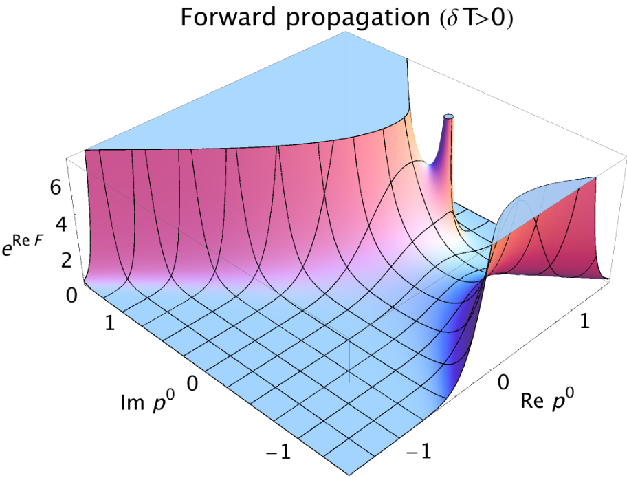
Figure 4: We plot eℜ⁡ℱe^{\Re\mathcal{F}} with sample parameters ς+=10\varsigma_{+}=10, ως​(𝒑∗)\omega_{\varsigma}\!\left(\boldsymbol{p}_{*}\right) (=ℜ⁡p∗0\Re p^{0}_{*}) =0.5=0.5, and ϵ=0.3\epsilon=0.3 in the E𝒑=1E_{\boldsymbol{p}}=1 units. This corresponds to forward propagation of Φ\Phi with δ​𝔗ς+{\delta\mathfrak{T}\over\varsigma_{+}} (=−ℑ⁡p∗0=-\Im p^{0}_{*}) =0.5=0.5.

Here, we evaluate the p0p^{0}-integral in Eq. (50) by the Lefschetz thimble decomposition to confirm Eq. (63). That is, we show that the result (63) can be understood as a Stokes phenomenon.

We first rewrite the integral (58) into an exponential form:

I⁡(𝒑)\displaystyle I\!\left(\boldsymbol{p}\right) =∫−∞∞d​p02​π​i​eℱ⁡(p0,𝒑),\displaystyle=\int_{-\infty}^{\infty}{\text{d}p^{0}\over 2\pi i}e^{\mathcal{F}\left(p^{0};\boldsymbol{p}\right)}, (87)

where

ℱ⁡(p0,𝒑)\displaystyle\mathcal{F}\!\left(p^{0};\boldsymbol{p}\right) =−ς+2​(p0−p∗0​(𝒑))2−ln⁡(−(p0)2+E𝒑2).\displaystyle=-{\varsigma_{+}\over 2}\left(p^{0}-p^{0}_{*}\!\left(\boldsymbol{p}\right)\right)^{2}-\ln\!\left(-\left(p^{0}\right)^{2}+\textbf{{E}}_{\boldsymbol{p}}^{2}\right). (88)

Recall that p∗0​(𝒑)p^{0}_{*}\!\left(\boldsymbol{p}\right) is given in Eq. (52). Hereafter, we suppress the 𝒑\boldsymbol{p}-dependence and write ℱ⁡(p0)\mathcal{F}\!\left(p^{0}\right), etc. for simplicity. As an illustration, we plot the absolute value of the integrand eℜ⁡ℱe^{\Re\mathcal{F}} on the complex p0p^{0} plane in Fig. 4, with sample parameters ς+=10\varsigma_{+}=10, ως​(𝒑∗)\omega_{\varsigma}\!\left(\boldsymbol{p}_{*}\right) (=ℜ⁡p∗0\Re p^{0}_{*}) =0.5=0.5, and ϵ=0.3\epsilon=0.3 in the E𝒑=1E_{\boldsymbol{p}}=1 units. The second logarithmic term in Eq. (88) modifies the exponent but the qualitative pole structure remains the same.

By solving ∂ℱ∂p0=0{\partial\mathcal{F}\over\partial p^{0}}=0, we obtain the three saddle points p(∗)0p^{0}_{(*)} and p(±)0p^{0}_{(\pm)} that are shifted from p∗0p^{0}_{*} and ±E𝒑\pm\textbf{{E}}_{\boldsymbol{p}} (see Fig. 3) due to the extra logarithmic term in ℱ⁡(p0)\mathcal{F}\!\left(p^{0}\right). Concretely, the saddle-point equation reads

∂ℱ∂p0\displaystyle{\partial\mathcal{F}\over\partial p^{0}} =−ς+​(p0−p∗0​(𝒑))−−2​p0−(p0)2+E𝒑2=0.\displaystyle=-\varsigma_{+}\left(p^{0}-p^{0}_{*}\!\left(\boldsymbol{p}\right)\right)-{-2p^{0}\over-\left(p^{0}\right)^{2}+\textbf{{E}}_{\boldsymbol{p}}^{2}}=0. (89)

This is cubic in p0p^{0}, and we obtain exact solutions for the saddle points p(i)0p^{0}_{(i)}. Here we show the large-ς+\varsigma_{+} results as an illustration, though we use the exact ones in the numerical plots below:

p(∗)0\displaystyle p^{0}_{(*)} ≃p∗0+1ς+​2​p∗0−(p∗0)2+E𝒑2,\displaystyle\simeq p^{0}_{*}+{1\over\varsigma_{+}}{{2p^{0}_{*}\over-\left(p^{0}_{*}\right)^{2}+\textbf{{E}}_{\boldsymbol{p}}^{2}}}, p(±)0\displaystyle p^{0}_{(\pm)} ≃±E𝒑+1ς+​1p∗0∓E𝒑,\displaystyle\simeq\pm\textbf{{E}}_{\boldsymbol{p}}+{1\over\varsigma_{+}}{{1\over p^{0}_{*}\mp\textbf{{E}}_{\boldsymbol{p}}}}, (90)

with

ℱ(∗)\displaystyle\mathcal{F}_{(*)} ≃ln⁡1−(p∗0)2+E𝒑2+1ς+​2​(p∗0)2((p∗0)2−E𝒑2)2,\displaystyle\simeq\ln{1\over-\left(p^{0}_{*}\right)^{2}+\textbf{{E}}_{\boldsymbol{p}}^{2}}+{1\over\varsigma_{+}}{2\left(p^{0}_{*}\right)^{2}\over\left(\left(p^{0}_{*}\right)^{2}-\textbf{{E}}_{\boldsymbol{p}}^{2}\right)^{2}}, (91)
ℱ(±)\displaystyle\mathcal{F}_{(\pm)} ≃−ς+2​(p∗0∓E𝒑)2+ln⁡(ς+2​(1∓p∗0E𝒑))+1,\displaystyle\simeq-{\varsigma_{+}\over 2}\left(p^{0}_{*}\mp\textbf{{E}}_{\boldsymbol{p}}\right)^{2}+\ln\!\left({\varsigma_{+}\over 2}\left(1\mp{p^{0}_{*}\over\textbf{{E}}_{\boldsymbol{p}}}\right)\right)+1, (92)

and

∂2ℱ(∗)∂p02\displaystyle{\partial^{2}\mathcal{F}_{(*)}\over{\partial p^{0}}^{2}} ≃−ς++1(p∗0+E𝒑)2+1(p∗0−E𝒑)2,\displaystyle\simeq-\varsigma_{+}+{1\over\left(p^{0}_{*}+\textbf{{E}}_{\boldsymbol{p}}\right)^{2}}+{1\over\left(p^{0}_{*}-\textbf{{E}}_{\boldsymbol{p}}\right)^{2}}, (93)
∂2ℱ(±)∂p02\displaystyle{\partial^{2}\mathcal{F}_{(\pm)}\over{\partial p^{0}}^{2}} ≃ς+2​(p∗0∓E𝒑)2−(2±p∗0E𝒑)​ς+,\displaystyle\simeq\varsigma_{+}^{2}\left(p^{0}_{*}\mp\textbf{{E}}_{\boldsymbol{p}}\right)^{2}-\left(2\pm{p^{0}_{*}\over\textbf{{E}}_{\boldsymbol{p}}}\right)\varsigma_{+}, (94)

where we have shown up to the sub-leading terms (as well as the order-ln⁡ς+\ln\varsigma_{+} term) for large ς+\varsigma_{+}.

For each saddle point (i)(i) with i=∗i=* and ±\pm, the steepest decent and ascent paths are obtained from the condition ℑ⁡(ℱ⁡(p0)−ℱ⁡(p(i)0))=0\Im\!\bigl(\mathcal{F}\!\left(p^{0}\right)-\mathcal{F}\!\bigl(p^{0}_{(i)}\bigr)\bigr)=0. The steepest descent path 𝒥(i)\mathcal{J}_{(i)} (ascent path 𝒦(i)\mathcal{K}_{(i)}) from the saddle point (i)(i) is called the Lefschetz thimble or the Stokes line (the anti-thimble or the anti-Stokes line). The integral path in the pole approach (a), which is one of the colored horizontal lines in Fig. 3, corresponds to 𝒥(∗)\mathcal{J}_{(*)} in the current approach (b). On the other hand, the poles ±E𝒑\pm\textbf{{E}}_{\boldsymbol{p}} in Fig. 3 correspond to the contour-integral along 𝒥(±)\mathcal{J}_{(\pm)}, respectively.

Refer to caption
Refer to caption
Refer to caption


Figure 5: We show contours for ℑ⁡ℱ=0\Im\mathcal{F}=0 (mod 2​π2\pi), on a density plot of ℜ⁡ℱ\Re\mathcal{F} in [−10,20][-10,20]. We have chosen sample parameters ς+=10\varsigma_{+}=10, ως​(𝒑∗)\omega_{\varsigma}\!\left(\boldsymbol{p}_{*}\right) (=ℜ⁡p∗0\Re p^{0}_{*}) =0.5=0.5, and ϵ=0.3\epsilon=0.3 in the E𝒑=1E_{\boldsymbol{p}}=1 units. The first panel corresponds to forward propagation of Φ\Phi with δ​𝔗ς+{\delta\mathfrak{T}\over\varsigma_{+}} (=−ℑ⁡p∗0=-\Im p^{0}_{*}) =0.5=0.5, while the second and third to equal-time and backward with δ​𝔗ς+=0{\delta\mathfrak{T}\over\varsigma_{+}}=0 and −0.5-0.5, respectively. The red-solid, yellow-dashed, and green-dotted contours are ℑ⁡ℱ=ℑ⁡ℱ(∗)\Im\mathcal{F}=\Im\mathcal{F}_{(*)}, ℑ⁡ℱ(+)\Im\mathcal{F}_{(+)}, and ℑ⁡ℱ(−)\Im\mathcal{F}_{(-)} respectively. The white dots denote the poles at p0=±E𝒑p^{0}=\pm\textbf{{E}}_{\boldsymbol{p}} and the blue single circles nearby them are correspondingly the saddle points p(±)0p^{0}_{(\pm)}. The blue double circle denotes the saddle point p(∗)0p^{0}_{(*)}.

As an illustration, we plot in Fig. 5 contours for ℑ⁡ℱ=0\Im\mathcal{F}=0 (mod 2​π2\pi), superimposed on the density plot for ℜ⁡ℱ\Re\mathcal{F}. The blue (double) circles denote saddle points p(i)0p^{0}_{(i)}, and the white dots denote the poles ±E𝒑\pm\textbf{{E}}_{\boldsymbol{p}}. The horizontal and vertical contours (both red-solid) through p(∗)0p^{0}_{(*)} are the thimble 𝒥(∗)\mathcal{J}_{(*)} and the anti-thimble 𝒦(∗)\mathcal{K}_{(*)}, respectively. Through p(+)0p^{0}_{(+)}, the yellow-dashed contour that connects E𝒑\textbf{{E}}_{\boldsymbol{p}} and a |ℑ⁡p0|→∞\left|\Im p^{0}\right|\to\infty region is the anti-thimble 𝒦(+)\mathcal{K}_{(+)}, while its perpendicular contour is the thimble 𝒥(+)\mathcal{J}_{(+)}. Through p(−)0p^{0}_{(-)}, the green-dotted contour connecting −E𝒑-\textbf{{E}}_{\boldsymbol{p}} and a |ℑ⁡p0|→∞\left|\Im p^{0}\right|\to\infty region is 𝒦(−)\mathcal{K}_{(-)}, and its perpendicular, 𝒥(−)\mathcal{J}_{(-)}. All the other contours that are disconnected from any of p(i)0p^{0}_{(i)} are irrelevant to the integral.

Refer to caption
Figure 6: Magnified plot for ℑ⁡ℱ\Im\mathcal{F} (mod 2​π2\pi) of the second panel in Fig. 5 near the saddle point p(−)0p^{0}_{(-)} (blue circle) and the pole −E𝒑-\textbf{{E}}_{\boldsymbol{p}} (white dot). We see that three contours and an artifact line terminate in −E𝒑-\textbf{{E}}_{\boldsymbol{p}}: The three contours are ℑ⁡ℱ=ℑ⁡ℱ(∗)\Im\mathcal{F}=\Im\mathcal{F}_{(*)} (red-solid), ℑ⁡ℱ=ℑ⁡ℱ(+)\Im\mathcal{F}=\Im\mathcal{F}_{(+)} (yellow-dashed), and the anti-thimble 𝒦(−)\mathcal{K}_{(-)} (green-dotted) from p(−)0p^{0}_{(-)}. The extra artifact line, seemingly consisting of three degenerate contours, is from the branch cut of the logarithmic function in the numerical computation, along which the contributions from all the other Riemann surfaces appear. This way, in each pole in Fig. 5, there always terminate three contours and an artifact line.

The figure is drawn on a single Riemann surface for the logarithmic function in ℱ⁡(p0)\mathcal{F}\!\left(p^{0}\right): In the case ℑ⁡p(∗)0≲ℑ⁡E𝒑\Im p^{0}_{(*)}\lesssim\Im\textbf{{E}}_{\boldsymbol{p}} in the first panel in Fig. 5, we may put a branch cut from −E𝒑-\textbf{{E}}_{\boldsymbol{p}} to −∞+ℑ⁡(−E𝒑)-\infty+\Im\!\left(-\textbf{{E}}_{\boldsymbol{p}}\right) and another from E𝒑\textbf{{E}}_{\boldsymbol{p}} along a, say, red-solid or green-dotted contour. This way, we may continuously deform ℝ\mathbb{R} into the thimbles 𝒥(∗)\mathcal{J}_{(*)} and 𝒥(+)\mathcal{J}_{(+)} without crossing the cuts. We may do similarly for other cases. In Fig. 6, we explain artifact lines appearing in Fig. 5 due to the branch cuts in the numerical computation.

We take the direction of 𝒥(±)\mathcal{J}_{(\pm)} such that it can be deformed to ℝ\mathbb{R} without crossing the poles, namely, 𝒥(+)\mathcal{J}_{(+)} and 𝒥(−)\mathcal{J}_{(-)} circulate E𝒑\textbf{{E}}_{\boldsymbol{p}} and −E𝒑-\textbf{{E}}_{\boldsymbol{p}} clockwise and counterclockwise, respectively. Along 𝒥(i)\mathcal{J}_{(i)}, we may evaluate the approximate Gaussian integral

I(i)​(𝒑)\displaystyle I_{(i)}\!\left(\boldsymbol{p}\right) =∫𝒥(i)d​p02​π​i​eℱ⁡(p0,𝒑)\displaystyle=\int_{\mathcal{J}_{(i)}}{\text{d}p^{0}\over 2\pi i}\,e^{\mathcal{F}\left(p^{0};\boldsymbol{p}\right)} (95)

without the oscillation of integrand:

I(∗)​(𝒑)\displaystyle I_{(*)}\!\left(\boldsymbol{p}\right) ≃12​π​ς+​−i−(p∗0​(𝒑))2+E𝒑2,\displaystyle\simeq{1\over\sqrt{2\pi\varsigma_{+}}}{-i\over-\left(p^{0}_{*}\!\left(\boldsymbol{p}\right)\right)^{2}+\textbf{{E}}_{\boldsymbol{p}}^{2}}, (96)
I(±)​(𝒑)\displaystyle I_{(\pm)}\!\left(\boldsymbol{p}\right) ≃∓−i2​π​1−ς+2​(p∗0​(𝒑)∓E𝒑)2​e−ς+2​(p∗0​(𝒑)∓E𝒑)2+1​ς+2​(1∓p∗0​(𝒑)E𝒑)=e2​π​e−ς+2​(p∗0​(𝒑)∓E𝒑)22​E𝒑,\displaystyle\simeq\mp{-i\over\sqrt{2\pi}}{1\over\sqrt{-\varsigma_{+}^{2}\left(p^{0}_{*}\!\left(\boldsymbol{p}\right)\mp\textbf{{E}}_{\boldsymbol{p}}\right)^{2}}}e^{-{\varsigma_{+}\over 2}\left(p^{0}_{*}\!\left(\boldsymbol{p}\right)\mp\textbf{{E}}_{\boldsymbol{p}}\right)^{2}+1}{\varsigma_{+}\over 2}\left(1\mp{p^{0}_{*}\!\left(\boldsymbol{p}\right)\over\textbf{{E}}_{\boldsymbol{p}}}\right)={e\over\sqrt{2\pi}}{e^{-{\varsigma_{+}\over 2}\left(p^{0}_{*}\!\left(\boldsymbol{p}\right)\mp\textbf{{E}}_{\boldsymbol{p}}\right)^{2}}\over 2\textbf{{E}}_{\boldsymbol{p}}}, (97)

where we have taken r​ei​θ=r​ei​θ/2\sqrt{re^{i\theta}}=\sqrt{r}e^{i\theta/2} for −π<θ<π-\pi<\theta<\pi, namely, (p∗0​(𝒑)∓E𝒑)2=E𝒑∓p∗0​(𝒑)\sqrt{\left(p^{0}_{*}\!\left(\boldsymbol{p}\right)\mp\textbf{{E}}_{\boldsymbol{p}}\right)^{2}}=\textbf{{E}}_{\boldsymbol{p}}\mp p^{0}_{*}\!\left(\boldsymbol{p}\right).

The integral II can be decomposed into those on the Lefschetz thimbles:

I=∑i=∗,±⟨𝒦(i),ℝ⟩I(i),\displaystyle I=\sum_{i=*,\pm}\Braket{\mathcal{K}_{(i)},\mathbb{R}}I_{(i)}, (98)

where ⟨𝒦(i),ℝ⟩\Braket{\mathcal{K}_{(i)},\mathbb{R}} is the intersection number between the anti-thimble 𝒦(i)\mathcal{K}_{(i)} and the original integration path ℝ\mathbb{R}; see e.g. Ref. [25] for a review. This expression allows an interpretation of the appearance of the Heaviside step functions in Eq. (63) as a Stokes phenomenon, which we discuss from now on.

There are three cases depending on the relative position of 𝒥(∗)\mathcal{J}_{(*)} and ±E𝒑\pm\textbf{{E}}_{\boldsymbol{p}}, represented in Fig. 5:

  1. (I)

    When ℑ⁡p(∗)0≲ℑ⁡E𝒑\Im p^{0}_{(*)}\lesssim\Im\textbf{{E}}_{\boldsymbol{p}} as in the first panel, the anti-thimble 𝒦(−)\mathcal{K}_{(-)} terminates in −E𝒑-\textbf{{E}}_{\boldsymbol{p}}, and hence do not intersect with the real axis: ⟨𝒦(−),ℝ⟩=0\Braket{\mathcal{K}_{(-)},\mathbb{R}}=0; see Fig. 6 for magnification and more explanation.

  2. (II)

    When ℑ⁡E𝒑≲ℑ⁡p(∗)0≲ℑ⁡(−E𝒑)\Im\textbf{{E}}_{\boldsymbol{p}}\lesssim\Im p^{0}_{(*)}\lesssim\Im\!\left(-\textbf{{E}}_{\boldsymbol{p}}\right) as in the second panel, both anti-thimbles terminate in ±E𝒑\pm\textbf{{E}}_{\boldsymbol{p}}, and hence ⟨𝒦(±),ℝ⟩=0\Braket{\mathcal{K}_{(\pm)},\mathbb{R}}=0.

  3. (III)

    When ℑ⁡p(∗)0≳ℑ⁡(−E𝒑)\Im p^{0}_{(*)}\gtrsim\Im\!\left(-\textbf{{E}}_{\boldsymbol{p}}\right) as in the third panel, 𝒦(+)\mathcal{K}_{(+)} terminates in E𝒑\textbf{{E}}_{\boldsymbol{p}}, and hence ⟨𝒦(+),ℝ⟩=0\Braket{\mathcal{K}_{(+)},\mathbb{R}}=0. This is how the discrete change in the amplitude (4) in the main text is understood as a Stokes phenomenon. Cases (I), (II), and (III) correspond to ℑ⁡p0<ℑ⁡E𝒑\Im p^{0}<\Im\textbf{{E}}_{\boldsymbol{p}}, ℑ⁡E𝒑<ℑ⁡p0<ℑ⁡(−E𝒑)\Im\textbf{{E}}_{\boldsymbol{p}}<\Im p^{0}<\Im\!\left(-\textbf{{E}}_{\boldsymbol{p}}\right), and ℑ⁡p0>ℑ⁡(−E𝒑)\Im p^{0}>\Im\!\left(-\textbf{{E}}_{\boldsymbol{p}}\right) in Approach (a), respectively.

We see that the results of Approaches (a) and (b) in Order 2, namely Eqs. (63) and (98), respectively obtained in this Sec. 4, are identical up to the extra factor e2​π≃1.08{e\over\sqrt{2\pi}}\simeq 1.08 that appears in Eq. (97).1313 13 It would be interesting to pursue the difference of the factor e/2​π≃1.08e/\sqrt{2\pi}\simeq 1.08 between Approaches (a) and (b). In the former, the saddle-point integral is done on the straight line, while in the latter, the integral on the thimble is approximated by the Gaussian integral on the straight line that is tangent to the thimble, which is highly bent in the limit ς+→∞\varsigma_{+}\to\infty. This might be a cause of the deviation.

4.3 Discussion on wave-packet Feynman propagator

We comment on the pole structure of the wave-packet Feynman propagator (60). From the dependence on δ​𝔗\delta\mathfrak{T} for a fixed ς+\varsigma_{+}, as well as on the energy difference such as E𝒑−ως​(𝒑)E_{\boldsymbol{p}}-\omega_{\varsigma}\!\left(\boldsymbol{p}\right), we identify the first term in Eq. (63) as the time-boundary effect, while the second and third ones as the bulk effect that has a counterpart in the plane-wave propagator: 1414 14 This is opposite to the interpretation in Ref. [21].

  • •

    In the first term, (i) the real and imaginary parts of the energy pole are shifted as E𝒑→E𝒑−ως​(𝒑)E_{\boldsymbol{p}}\to E_{\boldsymbol{p}}-\omega_{\varsigma}\!\left(\boldsymbol{p}\right) and −ϵ2​E𝒑→−ϵ2​E𝒑+δ​𝔗ς+-{\epsilon\over 2E_{\boldsymbol{p}}}\to-{\epsilon\over 2E_{\boldsymbol{p}}}+{\delta\mathfrak{T}\over\varsigma_{+}}, respectively; (ii) the energy non-conservation is suppressed only by a power law; and (iii) there is exponential suppression for large δ​𝔗\delta\mathfrak{T}. These are all the characteristics of the time boundary effect [20].

  • •

    In the second and third terms, (i) the pole structure 1E𝒑{1\over\textbf{{E}}_{\boldsymbol{p}}} is the same as the ordinary plane-wave propagator; (ii) the energy is exponentially localized to the positive and negative poles ως​(𝒑)≃E𝒑\omega_{\varsigma}\!\left(\boldsymbol{p}\right)\simeq\textbf{{E}}_{\boldsymbol{p}} and ως​(𝒑)≃−E𝒑\omega_{\varsigma}\!\left(\boldsymbol{p}\right)\simeq-\textbf{{E}}_{\boldsymbol{p}}, respectively; and (iii) when we first take the imaginary part infinitesimal as in the Feynman propagator, ℑ⁡E𝒑→0\Im\textbf{{E}}_{\boldsymbol{p}}\to 0, there is no exponential suppression for large δ​𝔗\delta\mathfrak{T}. These are all the characteristics of the bulk effect [20].

Historically in the original paper [5], Feynman first considered a transition amplitude between a wave packet that is time-translated from f⁡(𝒙1)f\!\left(\boldsymbol{x}_{1}\right) at t=0t=0 to TT (>0>0) and a wave packet g⁡(𝒙2)g\!\left(\boldsymbol{x}_{2}\right) at t=Tt=T under an external potential AA. Therefore the time integral over the interaction point in the resultant amplitudes (22) and (23) in Ref. [5] must be between 0 and TT 1515 15 This has to be the case unless we change the physical state to the “dressed” one in the sense of Ref. [21]. This change was made implicitly when Feynman gave the plane-wave amplitude in the momentum basis in the subsequent part in Ref. [5]. . Then he implicitly changed the time-boundary conditions to extract a manifestly Lorentz-covariant amplitude, corresponding to a transition from a plane wave at time −∞-\infty to a one at ∞\infty. In the sequel paper [6], he generalized this to many-body amplitudes “imagining that we can neglect the effect of interactions” near the time boundaries, hoping that “we do not lose much in a general theoretical sense by this approximation”; see also Ref. [26]. In the present paper, we calculate the amplitude including the time-boundary contribution that Feynman neglected. It is important that the wave-packet form (63) is a finite complete expression without any singularity and contains the plane-wave amplitude. We stress that the Gaussian basis forms a complete set that spans each free one-particle Hilbert space (see e.g. Refs. [22, 23]), and hence the time-boundary effect must not be omitted.1616 16 We comment that the standard textbook by Goldberger and Watson [27] also takes the same approach as that of Feynman, dropping the contributions from the asymptotic time region.

5 Summary

We have elucidated the nature of the wave-packet scattering amplitude ϕ​ϕ→Φ→ϕ​ϕ\phi\phi\to\Phi\to\phi\phi. The wave-packet formalism provides a finite amplitude-squared that has no ambiguity of the delta-function-squared of the energy-momentum, unlike the plane-wave amplitude-squared. The obtained amplitude provides a complete formula for the resonant production of Φ\Phi and its subsequent decay.

First, in Order 1, we have explicitly computed the wave-packet scattering amplitude relying on the saddle-point approximation in Sec. 3. We have proven that the in-time-boundary term for the Φ→ϕ​ϕ\Phi\to\phi\phi decay amplitude emerges from this scattering amplitude, even if we neglect both the in and out time boundaries for the ϕ​ϕ→ϕ​ϕ\phi\phi\to\phi\phi scattering process. For the first time, we have derived the time boundary term shown in Eq. (46) without introducing any time boundary a priori. We stress that our formula is applicable to the general situation, including the intermediate state Φ\Phi being long-lived.

Second, in Order 2, we have confirmed the result in the different integration order in Sec. 4. The confirmation is done in the two different approaches (a) saddle-point and poles and (b) Lefschetz thimble decomposition in Secs. 4.1 and 4.2, respectively. In Sec. 4.3, we discussed the relation to the ordinary plane-wave Feynman propagator in detail. The wave-packet amplitude contains more information than the plane-wave counterpart and exhibits the time-boundary effect, which is hardly tractable in the plane-wave formulation.

The time-boundary effect directly influences the transition probability, a critical element of quantum physics, and hence has a great impact on vast sectors of scientific study.

Acknowledgement

We thank Osamu Jinnouchi and Ryosuke Sato for the useful discussion and Juntaro Wada for reading the manuscript of the first draft. This work is in part supported by JSPS Kakenhi Grant Nos. 21H01107 (K.I., K.N., and K.O.) and 19H01899 (K.O.).

Appendix

Appendix A Notations

We list the symbols defined in the main text:

𝑽a\displaystyle\boldsymbol{V}_{a} =𝑷aEa=𝑷am2+𝑷a2,\displaystyle={\boldsymbol{P}_{a}\over E_{a}}={\boldsymbol{P}_{a}\over\sqrt{m^{2}+\boldsymbol{P}_{a}^{2}}}, (99)
E𝒑\displaystyle E_{\boldsymbol{p}} =M2+𝒑2,\displaystyle=\sqrt{M^{2}+\boldsymbol{p}^{2}}, E𝒑\displaystyle\textbf{{E}}_{\boldsymbol{p}} =E𝒑2−i​ϵ=M2+𝒑2−i​ϵ,\displaystyle=\sqrt{E_{\boldsymbol{p}}^{2}-i\epsilon}=\sqrt{M^{2}+\boldsymbol{p}^{2}-i\epsilon}, M =M2−i​ϵ,\displaystyle=\sqrt{M^{2}-i\epsilon}, (100)
Ein\displaystyle E_{\text{in}} =E1+E2,\displaystyle=E_{1}+E_{2}, Eout\displaystyle E_{\text{out}} =E3+E4,\displaystyle=E_{3}+E_{4}, (101)
𝑷in\displaystyle\boldsymbol{P}_{\text{in}} =𝑷1+𝑷2,\displaystyle=\boldsymbol{P}_{1}+\boldsymbol{P}_{2}, 𝑷out\displaystyle\boldsymbol{P}_{\text{out}} =𝑷3+𝑷4,\displaystyle=\boldsymbol{P}_{3}+\boldsymbol{P}_{4}, (102)
σin\displaystyle\sigma_{\text{in}} =11σ1+1σ2=σ1​σ2σ1+σ2,\displaystyle={1\over{1\over\sigma_{1}}+{1\over\sigma_{2}}}={\sigma_{1}\sigma_{2}\over\sigma_{1}+\sigma_{2}}, σout\displaystyle\sigma_{\text{out}} =11σ3+1σ4=σ3​σ4σ3+σ4,\displaystyle={1\over{1\over\sigma_{3}}+{1\over\sigma_{4}}}={\sigma_{3}\sigma_{4}\over\sigma_{3}+\sigma_{4}}, (103)
𝑽¯in\displaystyle\overline{\boldsymbol{V}}_{\text{in}} =σin​(𝑽1σ1+𝑽2σ2),\displaystyle=\sigma_{\text{in}}\left({\boldsymbol{V}_{1}\over\sigma_{1}}+{\boldsymbol{V}_{2}\over\sigma_{2}}\right), 𝑽¯out\displaystyle\overline{\boldsymbol{V}}_{\text{out}} =σout​(𝑽3σ3+𝑽4σ4),\displaystyle=\sigma_{\text{out}}\left({\boldsymbol{V}_{3}\over\sigma_{3}}+{\boldsymbol{V}_{4}\over\sigma_{4}}\right), (104)
ωin​(𝒑)\displaystyle\omega_{\text{in}}\!\left(\boldsymbol{p}\right) =Ein+𝑽¯in⋅(𝒑−𝑷in),\displaystyle=E_{\text{in}}+\overline{\boldsymbol{V}}_{\text{in}}\cdot\left(\boldsymbol{p}-\boldsymbol{P}_{\text{in}}\right), ωout​(𝒑)\displaystyle\omega_{\text{out}}\!\left(\boldsymbol{p}\right) =Eout+𝑽¯out⋅(𝒑−𝑷out),\displaystyle=E_{\text{out}}+\overline{\boldsymbol{V}}_{\text{out}}\cdot\left(\boldsymbol{p}-\boldsymbol{P}_{\text{out}}\right), (105)
ςin\displaystyle\varsigma_{\text{in}} =σ1+σ2(𝑽1−𝑽2)2,\displaystyle={\sigma_{1}+\sigma_{2}\over\left(\boldsymbol{V}_{1}-\boldsymbol{V}_{2}\right)^{2}}, ςout\displaystyle\varsigma_{\text{out}} =σ3+σ4(𝑽3−𝑽4)2,\displaystyle={\sigma_{3}+\sigma_{4}\over\left(\boldsymbol{V}_{3}-\boldsymbol{V}_{4}\right)^{2}}, (106)
σ\displaystyle\sigma =11σin+1σout=11σ1+1σ2+1σ3+1σ4,\displaystyle={1\over{1\over\sigma_{\text{in}}}+{1\over\sigma_{\text{out}}}}={1\over{1\over\sigma_{1}}+{1\over\sigma_{2}}+{1\over\sigma_{3}}+{1\over\sigma_{4}}}, σ+\displaystyle\sigma_{+} =σin+σout,\displaystyle=\sigma_{\text{in}}+\sigma_{\text{out}}, (107)
ς\displaystyle\varsigma =11ςin+1ςout=ςin​ςoutςin+ςout,\displaystyle={1\over{1\over\varsigma_{\text{in}}}+{1\over\varsigma_{\text{out}}}}={\varsigma_{\text{in}}\varsigma_{\text{out}}\over\varsigma_{\text{in}}+\varsigma_{\text{out}}}, ς+\displaystyle\varsigma_{+} =ςin+ςout,\displaystyle=\varsigma_{\text{in}}+\varsigma_{\text{out}}, (108)
Eσ\displaystyle E_{\sigma} =M2+𝑷σ2,\displaystyle=\sqrt{M^{2}+\boldsymbol{P}_{\sigma}^{2}}, Eσ\displaystyle\textbf{{E}}_{\sigma} =Eσ2−i​ϵ=M2+𝑷σ2−i​ϵ,\displaystyle=\sqrt{E_{\sigma}^{2}-i\epsilon}=\sqrt{M^{2}+\boldsymbol{P}_{\sigma}^{2}-i\epsilon}, (109)
ως​(𝒑)\displaystyle\omega_{\varsigma}\!\left(\boldsymbol{p}\right) =ςin​ωin​(𝒑)+ςout​ωout​(𝒑)ςin+ςout,\displaystyle={\varsigma_{\text{in}}\omega_{\text{in}}\!\left(\boldsymbol{p}\right)+\varsigma_{\text{out}}\omega_{\text{out}}\!\left(\boldsymbol{p}\right)\over\varsigma_{\text{in}}+\varsigma_{\text{out}}}, Eς\displaystyle E_{\varsigma} =ςin​Ein+ςout​Eoutςin+ςout,\displaystyle={\varsigma_{\text{in}}E_{\text{in}}+\varsigma_{\text{out}}E_{\text{out}}\over\varsigma_{\text{in}}+\varsigma_{\text{out}}}, (110)
δ​𝚵¯\displaystyle\delta\overline{\boldsymbol{\Xi}} =𝚵¯out−𝚵¯in,\displaystyle=\overline{\boldsymbol{\Xi}}_{\text{out}}-\overline{\boldsymbol{\Xi}}_{\text{in}}, δ​𝔗\displaystyle\delta\mathfrak{T} =𝔗out-int−𝔗in-int,\displaystyle=\mathfrak{T}_{\text{out-int}}-\mathfrak{T}_{\text{in-int}}, (111)
Δ​T\displaystyle\Delta\textbf{{T}} =δ​𝔗+ς+​ℑ⁡Eσ+i​ςout​(Eout−ℜ⁡Eσ),\displaystyle=\delta\mathfrak{T}+\varsigma_{+}\Im\textbf{{E}}_{\sigma}+i\varsigma_{\text{out}}\left(E_{\text{out}}-\Re\textbf{{E}}_{\sigma}\right), (112)
N\displaystyle N =(−i​κ)2​e−ℛin+ℛout2​∏a=1412​Ea​(1π​σa)3/4,\displaystyle=\left(-i\kappa\right)^{2}e^{-{\mathcal{R}_{\text{in}}+\mathcal{R}_{\text{out}}\over 2}}\prod_{a=1}^{4}{1\over\sqrt{2E_{a}}}\left({1\over\pi\sigma_{a}}\right)^{3/4}, (113)
sin\displaystyle\textsf{s}_{\text{in}} :=11ςin+𝑽¯in2σ+,\displaystyle:={1\over{1\over\varsigma_{\text{in}}}+{\overline{\boldsymbol{V}}_{\text{in}}^{2}\over\sigma_{+}}}, (114)
sout\displaystyle\textsf{s}_{\text{out}} :=ςout1+ςoutσ+​(𝑽¯out2−sin​(𝑽¯in⋅𝑽¯out)2σ+),\displaystyle:={\varsigma_{\text{out}}\over 1+{\varsigma_{\text{out}}\over\sigma_{+}}\left(\overline{\boldsymbol{V}}_{\text{out}}^{2}-{\textsf{s}_{\text{in}}\left(\overline{\boldsymbol{V}}_{\text{in}}\cdot\overline{\boldsymbol{V}}_{\text{out}}\right)^{2}\over\sigma_{+}}\right)}, (115)
Tin-int±\displaystyle\textbf{{T}}_{\text{in-int}}^{\pm} :=sin​{[𝔗in-intςin+𝑽¯in⋅δ​𝚵¯σ+]−i⁡[ωin​(0)∓Eσ+σ​𝑽¯in⋅(𝑷out−𝑷in)σin]},\displaystyle:=\textsf{s}_{\text{in}}\left\{\left[{\mathfrak{T}_{\text{in-int}}\over\varsigma_{\text{in}}}+{\overline{\boldsymbol{V}}_{\text{in}}\cdot\delta\overline{\boldsymbol{\Xi}}\over\sigma_{+}}\right]-i\left[\omega_{\text{in}}\!\left(0\right)\mp\textbf{{E}}_{\sigma}+{\sigma\overline{\boldsymbol{V}}_{\text{in}}\cdot\left(\boldsymbol{P}_{\text{out}}-\boldsymbol{P}_{\text{in}}\right)\over\sigma_{\text{in}}}\right]\right\}, (116)
Tout-int±\displaystyle\textbf{{T}}_{\text{out-int}}^{\pm} :=sout{[𝔗out-intςout+𝑽¯out⋅(𝑽¯in​Tin-int−δ​𝚵¯)σ+]\displaystyle:=\textsf{s}_{\text{out}}\Bigg\{\left[{\mathfrak{T}_{\text{out-int}}\over\varsigma_{\text{out}}}+{\overline{\boldsymbol{V}}_{\text{out}}\cdot\left(\overline{\boldsymbol{V}}_{\text{in}}\textbf{{T}}_{\text{in-int}}-\delta\overline{\boldsymbol{\Xi}}\right)\over\sigma_{+}}\right]
+i[ωout(0)∓Eσ(1−sin​𝑽¯in⋅𝑽¯outσ+)−σ​𝑽¯out⋅(𝑷out−𝑷in)σout]},\displaystyle\phantom{:=\textsf{s}_{\text{out}}\Bigg\{}+i\left[\omega_{\text{out}}\!\left(0\right)\mp\textbf{{E}}_{\sigma}\left(1-{\textsf{s}_{\text{in}}\overline{\boldsymbol{V}}_{\text{in}}\cdot\overline{\boldsymbol{V}}_{\text{out}}\over\sigma_{+}}\right)-{\sigma\overline{\boldsymbol{V}}_{\text{out}}\cdot\left(\boldsymbol{P}_{\text{out}}-\boldsymbol{P}_{\text{in}}\right)\over\sigma_{\text{out}}}\right]\Bigg\}, (117)
𝑽¯σ\displaystyle\overline{\boldsymbol{V}}_{\sigma} :=σ⁡(𝑽¯inσin+𝑽¯outσout),\displaystyle:=\sigma\left({\overline{\boldsymbol{V}}_{\text{in}}\over\sigma_{\text{in}}}+{\overline{\boldsymbol{V}}_{\text{out}}\over\sigma_{\text{out}}}\right), 𝑽¯ς\displaystyle\overline{\boldsymbol{V}}_{\varsigma} :=ςin​𝑽¯in+ςout​𝑽¯outςin+ςout,\displaystyle:={\varsigma_{\text{in}}\overline{\boldsymbol{V}}_{\text{in}}+\varsigma_{\text{out}}\overline{\boldsymbol{V}}_{\text{out}}\over\varsigma_{\text{in}}+\varsigma_{\text{out}}}, 𝔗ς\displaystyle\mathfrak{T}_{\varsigma} :=ς⁡(𝔗in-intςin+𝔗out-intςout),\displaystyle:=\varsigma\left({\mathfrak{T}_{\text{in-int}}\over\varsigma_{\text{in}}}+{\mathfrak{T}_{\text{out-int}}\over\varsigma_{\text{out}}}\right), (118)
Eς\displaystyle E_{\varsigma} :=ςin​Ein+ςout​Eoutςin+ςout,\displaystyle:={\varsigma_{\text{in}}E_{\text{in}}+\varsigma_{\text{out}}E_{\text{out}}\over\varsigma_{\text{in}}+\varsigma_{\text{out}}}, (119)
δ​ω​(𝒑)\displaystyle\delta\omega\!\left(\boldsymbol{p}\right) :=ωout​(𝒑)−ωin​(𝒑),\displaystyle:=\omega_{\text{out}}\!\left(\boldsymbol{p}\right)-\omega_{\text{in}}\!\left(\boldsymbol{p}\right), (120)
δ​𝚵¯\displaystyle\delta\overline{\boldsymbol{\Xi}} :=𝚵¯out−𝚵¯in,\displaystyle:=\overline{\boldsymbol{\Xi}}_{\text{out}}-\overline{\boldsymbol{\Xi}}_{\text{in}}, (121)
δ​𝔗\displaystyle\delta\mathfrak{T} :=𝔗out-int−𝔗in-int,\displaystyle:=\mathfrak{T}_{\text{out-int}}-\mathfrak{T}_{\text{in-int}}, (122)
Δ​T\displaystyle\Delta\!\textbf{{T}} :=δ​𝔗+ςout​ℑ⁡Eσ+i​ςout​(Eout−ℜ⁡Eσ).\displaystyle:=\delta\mathfrak{T}+\varsigma_{\text{out}}\Im\textbf{{E}}_{\sigma}+i\varsigma_{\text{out}}\left(E_{\text{out}}-\Re\textbf{{E}}_{\sigma}\right). (123)

Appendix B Expressions for simplifying configuration

We list expressions for the simplifying configuration (41).

  • •

    Eqs. (23) and (24):

    ℐ ​(x0,y0)\displaystyle\mathcal{I}_{\text{\faIconFromMacro{faStarO}}}\!\left(x^{0},y^{0}\right) →∫d​p02​π​i​e−i​p0​(y0−x0)−(p0)2+𝑷σ2+M2−(δ​𝚵¯)2σ+2−i⁡(ϵ−2​𝑷σ⋅δ​𝚵¯σ+),\displaystyle\to\int{\text{d}p^{0}\over 2\pi i}{e^{-ip^{0}\left(y^{0}-x^{0}\right)}\over-\left(p^{0}\right)^{2}+\boldsymbol{P}_{\sigma}^{2}+M^{2}-{(\delta\overline{\boldsymbol{\Xi}})^{2}\over\sigma_{+}^{2}}-i\left(\epsilon-{2\boldsymbol{P}_{\sigma}\cdot\delta\overline{\boldsymbol{\Xi}}\over\sigma_{+}}\right)}, (124)
    V ​(x0,y0)\displaystyle V_{\text{\faIconFromMacro{faStarO}}}\!\left(x^{0},y^{0}\right) →−σ2​(𝑷out−𝑷in)2−12​σ+​(𝚵¯out−𝚵¯in)2−i​𝚵¯σ⋅(𝑷out−𝑷in)−i​ωin​(0)​x0+i​ωout​(0)​y0.\displaystyle\to-{\sigma\over 2}\left(\boldsymbol{P}_{\text{out}}-\boldsymbol{P}_{\text{in}}\right)^{2}-{1\over 2\sigma_{+}}\left(\overline{\boldsymbol{\Xi}}_{\text{out}}-\overline{\boldsymbol{\Xi}}_{\text{in}}\right)^{2}-i\overline{\boldsymbol{\Xi}}_{\sigma}\cdot\left(\boldsymbol{P}_{\text{out}}-\boldsymbol{P}_{\text{in}}\right)-i\omega_{\text{in}}\!\left(0\right)x^{0}+i\omega_{\text{out}}\!\left(0\right)y^{0}. (125)
  • •

    Eq. (29):

    𝒮\displaystyle\mathcal{S} →(2​π​σ)3/2​N2​Eσ​e−σ2​(𝑷out−𝑷in)2−12​σ+​(𝚵¯out−𝚵¯in)2−i​𝚵¯σ⋅(𝑷out−𝑷in)\displaystyle\to{\left(2\pi\sigma\right)^{3/2}N\over 2\textbf{{E}}_{\sigma}}e^{-{\sigma\over 2}\left(\boldsymbol{P}_{\text{out}}-\boldsymbol{P}_{\text{in}}\right)^{2}-{1\over 2\sigma_{+}}\left(\overline{\boldsymbol{\Xi}}_{\text{out}}-\overline{\boldsymbol{\Xi}}_{\text{in}}\right)^{2}-i\overline{\boldsymbol{\Xi}}_{\sigma}\cdot\left(\boldsymbol{P}_{\text{out}}-\boldsymbol{P}_{\text{in}}\right)}
    ×∫−∞∞d​y0​e−12​ςout​(y0−𝔗out-int)2+i​Eout​y0−𝔗in-int22​ςin\displaystyle\quad\times\int_{-\infty}^{\infty}\text{d}y^{0}\,e^{-{1\over 2\varsigma_{\text{out}}}\left(y^{0}-\mathfrak{T}_{\text{out-int}}\right)^{2}+iE_{\text{out}}y^{0}-{\mathfrak{T}_{\text{in-int}}^{2}\over 2\varsigma_{\text{in}}}}
    ×2​π​ςin[e12​ςin​(𝔗in-int+i​ςin​(Eσ−Ein))2−i​Eσ​y01+erf⁡(y0−𝔗in-int−i​ςin​(Eσ−Ein)2​ςin)2\displaystyle\quad\times\sqrt{2\pi\varsigma_{\text{in}}}\left[e^{{1\over 2\varsigma_{\text{in}}}\left({\mathfrak{T}_{\text{in-int}}}+i\varsigma_{\text{in}}\bigl(\textbf{{E}}_{\sigma}-E_{\text{in}}\bigr)\right)^{2}-i\textbf{{E}}_{\sigma}y^{0}}{1+\erf\!\left(y^{0}-{\mathfrak{T}_{\text{in-int}}}-i\varsigma_{\text{in}}\bigl(\textbf{{E}}_{\sigma}-E_{\text{in}}\bigr)\over\sqrt{2\varsigma_{\text{in}}}\right)\over 2}\right.
    +e12​ςin​(𝔗in-int−i​ςin​(Eσ+Ein))2+i​Eσ​y01+erf⁡(𝔗in-int−i​ςin​(Eσ+Ein)−y02​ςin)2].\displaystyle\phantom{\quad\times\sqrt{2\pi\varsigma_{\text{in}}}\Bigg[}\left.\mbox{}+e^{{1\over 2\varsigma_{\text{in}}}\left({\mathfrak{T}_{\text{in-int}}}-i\varsigma_{\text{in}}\bigl(\textbf{{E}}_{\sigma}+E_{\text{in}}\bigr)\right)^{2}+i\textbf{{E}}_{\sigma}y^{0}}{1+\erf\!\left({\mathfrak{T}_{\text{in-int}}}-i\varsigma_{\text{in}}\bigl(\textbf{{E}}_{\sigma}+E_{\text{in}}\bigr)-y^{0}\over\sqrt{2\varsigma_{\text{in}}}\right)\over 2}\right]. (126)
  • •

    Eq. (37):

    S\displaystyle S →(2​π​σ)3/2​N2​Eσ​e−σ2​(𝑷out−𝑷in)2−12​σ+​(𝚵¯out−𝚵¯in)2−i​𝚵¯σ⋅(𝑷out−𝑷in)+i​Eout​𝔗out-int−i​Ein​𝔗in-int​2​π​ςin​2​π​ςout\displaystyle\to{\left(2\pi\sigma\right)^{3/2}N\over 2\textbf{{E}}_{\sigma}}e^{-{\sigma\over 2}\left(\boldsymbol{P}_{\text{out}}-\boldsymbol{P}_{\text{in}}\right)^{2}-{1\over 2\sigma_{+}}\left(\overline{\boldsymbol{\Xi}}_{\text{out}}-\overline{\boldsymbol{\Xi}}_{\text{in}}\right)^{2}-i\overline{\boldsymbol{\Xi}}_{\sigma}\cdot\left(\boldsymbol{P}_{\text{out}}-\boldsymbol{P}_{\text{in}}\right)+iE_{\text{out}}\mathfrak{T}_{\text{out-int}}-iE_{\text{in}}\mathfrak{T}_{\text{in-int}}}\sqrt{2\pi\varsigma_{\text{in}}}\sqrt{2\pi\varsigma_{\text{out}}}
    ×[e−ςin​(Eσ−Ein)22−ςout​(Eout−Eσ)22−i​Eσ​δ​𝔗(θ(δ𝔗+ς+ℑEσ)+erf⁡(Δ​T2​ςout)−sgn⁡(Δ​T2​ςout)2)\displaystyle\quad\times\Bigg[e^{-{\varsigma_{\text{in}}\left(\textbf{{E}}_{\sigma}-E_{\text{in}}\right)^{2}\over 2}-{\varsigma_{\text{out}}\left(E_{\text{out}}-\textbf{{E}}_{\sigma}\right)^{2}\over 2}-i\textbf{{E}}_{\sigma}\delta\mathfrak{T}}\left(\theta\!\left(\delta\mathfrak{T}+\varsigma_{+}\Im\textbf{{E}}_{\sigma}\right)+{\erf\!\left(\Delta\textbf{{T}}\over\sqrt{2\varsigma_{\text{out}}}\right)-\sgn\!\left(\Delta\textbf{{T}}\over\sqrt{2\varsigma_{\text{out}}}\right)\over 2}\right)
    +e−ςin​(Eσ+Ein)22−ςout​(Eout+Eσ)22+i​Eσ​δ​𝔗\displaystyle\phantom{\quad\times\Bigg[}+e^{-{\varsigma_{\text{in}}\left(\textbf{{E}}_{\sigma}+E_{\text{in}}\right)^{2}\over 2}-{\varsigma_{\text{out}}\left(E_{\text{out}}+\textbf{{E}}_{\sigma}\right)^{2}\over 2}+i\textbf{{E}}_{\sigma}\delta\mathfrak{T}}
    ×(θ(−δ𝔗+ς+ℑEσ)+erf⁡(−δ​𝔗+ς+​ℑ⁡Eσ−i​ςout​(Eout+ℜ⁡Eσ)2​ςout)−sgn⁡(−δ​𝔗+ς+​ℑ⁡Eσ−i​ςout​(Eout+ℜ⁡Eσ)2​ςout)2)].\displaystyle\phantom{\quad\times\Bigg[+}\times\left(\theta\!\left(-\delta\mathfrak{T}+\varsigma_{+}\Im\textbf{{E}}_{\sigma}\right)+{\erf\!\left(-\delta\mathfrak{T}+\varsigma_{+}\Im\textbf{{E}}_{\sigma}-i\varsigma_{\text{out}}\left(E_{\text{out}}+\Re\textbf{{E}}_{\sigma}\right)\over\sqrt{2\varsigma_{\text{out}}}\right)-\sgn\!\left(-\delta\mathfrak{T}+\varsigma_{+}\Im\textbf{{E}}_{\sigma}-i\varsigma_{\text{out}}\left(E_{\text{out}}+\Re\textbf{{E}}_{\sigma}\right)\over\sqrt{2\varsigma_{\text{out}}}\right)\over 2}\right)\Bigg]. (127)
  • •

    Eq. (38):

    →θ⁡(δ​𝔗+ς+​ℑ⁡Eσ).\displaystyle\to\theta\!\left(\delta\mathfrak{T}+\varsigma_{+}\Im\textbf{{E}}_{\sigma}\right). (128)
  • •

    Eq. (39):

    →θ⁡(−δ​𝔗+ς+​ℑ⁡Eσ).\displaystyle\to\theta\!\left(-\delta\mathfrak{T}+\varsigma_{+}\Im\textbf{{E}}_{\sigma}\right). (129)

Appendix C Details on Fig. 2

In Fig. 2, we have plotted |𝒮|2\left|\mathcal{S}\right|^{2} (up to the normalization factor (152) below), using Eq. (46), as a function of final state positions

x3\displaystyle x_{3} :=|𝑿3|,\displaystyle:=\left|\boldsymbol{X}_{3}\right|, x4\displaystyle x_{4} :=|𝑿4|.\displaystyle:=\left|\boldsymbol{X}_{4}\right|. (130)

We have focused on the back-to-back scattering in the center-of-mass frame,

𝑷in\displaystyle\boldsymbol{P}_{\text{in}} :=𝑷1+𝑷2=0,\displaystyle:=\boldsymbol{P}_{1}+\boldsymbol{P}_{2}=0, 𝑷out\displaystyle\boldsymbol{P}_{\text{out}} :=𝑷3+𝑷4=0,\displaystyle:=\boldsymbol{P}_{3}+\boldsymbol{P}_{4}=0, |𝑷1|\displaystyle\left|\boldsymbol{P}_{1}\right| =|𝑷2|=|𝑷3|=|𝑷4|(=|𝑷|),\displaystyle=\left|\boldsymbol{P}_{2}\right|=\left|\boldsymbol{P}_{3}\right|=\left|\boldsymbol{P}_{4}\right|\quad\bigl(\,=\left|\boldsymbol{P}\right|\,\bigr), (131)

with the wave-packet positions being collinear to their momenta, 𝑿a∝𝑷a\boldsymbol{X}_{a}\propto\boldsymbol{P}_{a} (=Ea​𝑽a=E_{a}\boldsymbol{V}_{a}; a=1,…,4a=1,\dots,4), and overlapping at the origin:

𝚵1\displaystyle\boldsymbol{\Xi}_{1} =𝑿1−𝑽1​(−T)=0,\displaystyle=\boldsymbol{X}_{1}-\boldsymbol{V}_{1}\left(-T\right)=0, 𝚵3\displaystyle\boldsymbol{\Xi}_{3} =(x3−T)​𝑽,\displaystyle=\left(x_{3}-T\right)\boldsymbol{V}, (132)
𝚵2\displaystyle\boldsymbol{\Xi}_{2} =−𝑿1−(−𝑽1)​(−T)=0,\displaystyle=-\boldsymbol{X}_{1}-\left(-\boldsymbol{V}_{1}\right)\left(-T\right)=0, 𝚵4\displaystyle\boldsymbol{\Xi}_{4} =(−x4+T)​𝑽,\displaystyle=\left(-x_{4}+T\right)\boldsymbol{V}, (133)

where

𝑽\displaystyle\boldsymbol{V} :=𝑽3=−𝑽4,\displaystyle:=\boldsymbol{V}_{3}=-\boldsymbol{V}_{4}, 𝑷\displaystyle\boldsymbol{P} :=𝑷3=−𝑷4,\displaystyle:=\boldsymbol{P}_{3}=-\boldsymbol{P}_{4}, (𝑽CLOSE\displaystyle\bigg(\,\boldsymbol{V} =𝑷m2+𝑷2,)\displaystyle={\boldsymbol{P}\over\sqrt{m^{2}+\boldsymbol{P}^{2}}},\,\bigg) (134)

and the initial and final times of the wave packets are taken to be T1=T2=−TT_{1}=T_{2}=-T and T3=T4=TT_{3}=T_{4}=T, respectively. It follows that |𝑽1|=|𝑽2|=|𝑽3|=|𝑽4|=|𝑽|\left|\boldsymbol{V}_{1}\right|=\left|\boldsymbol{V}_{2}\right|=\left|\boldsymbol{V}_{3}\right|=\left|\boldsymbol{V}_{4}\right|=\left|\boldsymbol{V}\right|. The widths of the wave packets are chosen to be symmetric σ1=σ2≪σ3=σ4\sigma_{1}=\sigma_{2}\ll\sigma_{3}=\sigma_{4}. As a result, we obtain

Ein\displaystyle E_{\text{in}} =2​m2+𝑷2,\displaystyle=2\sqrt{m^{2}+\boldsymbol{P}^{2}}, Eout\displaystyle E_{\text{out}} =2​m2+𝑷2,\displaystyle=2\sqrt{m^{2}+\boldsymbol{P}^{2}}, (135)
σin\displaystyle\sigma_{\text{in}} =σ12,\displaystyle={\sigma_{1}\over 2}, σout\displaystyle\sigma_{\text{out}} =σ32,\displaystyle={\sigma_{3}\over 2}, (136)
𝑽¯in\displaystyle\overline{\boldsymbol{V}}_{\text{in}} =0,\displaystyle=0, 𝑽¯out\displaystyle\overline{\boldsymbol{V}}_{\text{out}} =0,\displaystyle=0, (137)
ωin​(𝒑)\displaystyle\omega_{\text{in}}\!\left(\boldsymbol{p}\right) =Ein=2​m2+𝑷2,\displaystyle=E_{\text{in}}=2\sqrt{m^{2}+\boldsymbol{P}^{2}}, ωout​(𝒑)\displaystyle\omega_{\text{out}}\!\left(\boldsymbol{p}\right) =Eout=2​m2+𝑷2,\displaystyle=E_{\text{out}}=2\sqrt{m^{2}+\boldsymbol{P}^{2}}, (138)
ςin\displaystyle\varsigma_{\text{in}} =σ12​𝑽2,\displaystyle={\sigma_{1}\over 2\boldsymbol{V}^{2}}, ςout\displaystyle\varsigma_{\text{out}} =σ32​𝑽2,\displaystyle={\sigma_{3}\over 2\boldsymbol{V}^{2}}, (139)
σ\displaystyle\sigma ≃σ12,\displaystyle\simeq{\sigma_{1}\over 2}, σ+\displaystyle\sigma_{+} ≃σ32,\displaystyle\simeq{\sigma_{3}\over 2}, (140)
ς\displaystyle\varsigma ≃σ12​𝑽2,\displaystyle\simeq{\sigma_{1}\over 2\boldsymbol{V}^{2}}, ς+\displaystyle\varsigma_{+} ≃σ32​𝑽2,\displaystyle\simeq{\sigma_{3}\over 2\boldsymbol{V}^{2}}, (141)
𝑷σ\displaystyle\boldsymbol{P}_{\sigma} =0,\displaystyle=0, Eσ\displaystyle E_{\sigma} =M,\displaystyle=M, Eσ\displaystyle\textbf{{E}}_{\sigma} =M−i​ϵ2​M,\displaystyle=M-i{\epsilon\over 2M}, ℑ⁡Eσ\displaystyle\Im\textbf{{E}}_{\sigma} =−ϵ2​M,\displaystyle=-{\epsilon\over 2M}, (142)
ως​(𝒑)\displaystyle\omega_{\varsigma}\!\left(\boldsymbol{p}\right) =2​m2+𝑷2,\displaystyle=2\sqrt{m^{2}+\boldsymbol{P}^{2}}, Eς\displaystyle E_{\varsigma} =2​m2+𝑷2,\displaystyle=2\sqrt{m^{2}+\boldsymbol{P}^{2}}, (143)
𝑷out−𝑷in\displaystyle\boldsymbol{P}_{\text{out}}-\boldsymbol{P}_{\text{in}} =0,\displaystyle=0, Eout−Ein\displaystyle E_{\text{out}}-E_{\text{in}} =0,\displaystyle=0, (144)
δ​𝚵¯\displaystyle\delta\overline{\boldsymbol{\Xi}} =𝚵¯out=x3−x42​𝑽,\displaystyle=\overline{\boldsymbol{\Xi}}_{\text{out}}={x_{3}-x_{4}\over 2}\boldsymbol{V}, δ​𝔗\displaystyle\delta\mathfrak{T} =𝔗out-int=T−x3+x42,\displaystyle=\mathfrak{T}_{\text{out-int}}=T-{x_{3}+x_{4}\over 2}, (145)
Δ​T\displaystyle\Delta\textbf{{T}} ≃T−x3+x42−ϵ​σ34​M​𝑽2+i​σ32​𝑽2​(2​m2+𝑷2−M),\displaystyle\simeq T-{x_{3}+x_{4}\over 2}-{\epsilon\sigma_{3}\over 4M\boldsymbol{V}^{2}}+i{\sigma_{3}\over 2\boldsymbol{V}^{2}}\left(2\sqrt{m^{2}+\boldsymbol{P}^{2}}-M\right), (146)
N\displaystyle N =−κ2​1(2​E1)2​(1π​σ1)3/2​(1π​σ3)3/2,\displaystyle=-\kappa^{2}{1\over\left(2E_{1}\right)^{2}}\left({1\over\pi\sigma_{1}}\right)^{3/2}\left({1\over\pi\sigma_{3}}\right)^{3/2}, (147)

where we have taken a small ϵ\epsilon and

𝚵¯in\displaystyle\overline{\boldsymbol{\Xi}}_{\text{in}} =0,\displaystyle=0, 𝚵¯out\displaystyle\overline{\boldsymbol{\Xi}}_{\text{out}} =x3−x42​𝑽,\displaystyle={x_{3}-x_{4}\over 2}\boldsymbol{V}, (148)
𝔗in-int\displaystyle\mathfrak{T}_{\text{in-int}} =0,\displaystyle=0, 𝔗out-int\displaystyle\mathfrak{T}_{\text{out-int}} =T−x3+x42,\displaystyle=T-{x_{3}+x_{4}\over 2}, (149)
ℛin\displaystyle\mathcal{R}_{\text{in}} =0,\displaystyle=0, ℛout\displaystyle\mathcal{R}_{\text{out}} =0.\displaystyle=0. (150)

The resultant expression for |𝒮|2\left|\mathcal{S}\right|^{2} is

|𝒮|2\displaystyle\left|\mathcal{S}\right|^{2} =C​M4|𝑷|4​e−𝑽22​σ3​(x3−x4)2−σ32​𝑽2​(2​m2+𝑷2−M)2\displaystyle=C{M^{4}\over\left|\boldsymbol{P}\right|^{4}}e^{-{\boldsymbol{V}^{2}\over 2\sigma_{3}}\left(x_{3}-x_{4}\right)^{2}-{\sigma_{3}\over 2\boldsymbol{V}^{2}}\left(2\sqrt{m^{2}+\boldsymbol{P}^{2}}-M\right)^{2}}
×|θ⁡(T−x3+x42−ϵ​σ34​M​𝑽2)+erf⁡(|𝑽|​Δ​Tσ3)−sgn⁡(|𝑽|​Δ​Tσ3)2|2,\displaystyle\quad\times\left|\theta\!\left(T-{x_{3}+x_{4}\over 2}-{\epsilon\sigma_{3}\over 4M\boldsymbol{V}^{2}}\right)+{\erf\!\left({\left|\boldsymbol{V}\right|\Delta\!\textbf{{T}}\over\sqrt{\sigma_{3}}}\right)-\sgn\!\left({\left|\boldsymbol{V}\right|\Delta\!\textbf{{T}}\over\sqrt{\sigma_{3}}}\right)\over 2}\right|^{2}, (151)

with Δ​T\Delta\!\textbf{{T}} being given by Eq. (146) and

C\displaystyle C :=κ464​π​M6​σ1σ32\displaystyle:={\kappa^{4}\over 64\pi M^{6}}{\sigma_{1}\over\sigma_{3}^{2}} (152)

is a constant factor. In FIG. 2 in the main text, we have plotted |𝒮|2/C\left|\mathcal{S}\right|^{2}/C.

The plot is for the parameters

m\displaystyle m =M4,\displaystyle={M\over 4}, T\displaystyle T =100M,\displaystyle={100\over M}, ϵ\displaystyle\epsilon =0.01​M2,\displaystyle=0.01M^{2}, σ3\displaystyle\sigma_{3} =10M2.\displaystyle={10\over M^{2}}. (153)

On the upper panels, we have chosen the momenta to be on the resonance:

2​m2+𝑷2=M,\displaystyle 2\sqrt{m^{2}+\boldsymbol{P}^{2}}=M, (154)

namely, |𝑷|=34​M\left|\boldsymbol{P}\right|={\sqrt{3}\over 4}M. On the lower panels, we have chosen them to be off the resonance: |𝑷|=M4\left|\boldsymbol{P}\right|={M\over 4}.

On the left panels, we include only the first term in the absolute squared in Eq. (151), namely,

∝{θ⁡(T−x3+x42−ϵ​σ34​M​𝑽2)}2.\displaystyle\propto\left\{\theta\!\left(T-{x_{3}+x_{4}\over 2}-{\epsilon\sigma_{3}\over 4M\boldsymbol{V}^{2}}\right)\right\}^{2}. (155)

On the right panels, we take into account all the contributions including the interference with the boundary contribution

∝θ⁡(T−x3+x42−ϵ​σ34​M​𝑽2)​(erf⁡(|𝑽|​Δ​Tσ3)−sgn⁡(|𝑽|​Δ​Tσ3)2+h.c.)\displaystyle\propto\theta\!\left(T-{x_{3}+x_{4}\over 2}-{\epsilon\sigma_{3}\over 4M\boldsymbol{V}^{2}}\right)\left({\erf\!\left({\left|\boldsymbol{V}\right|\Delta\!\textbf{{T}}\over\sqrt{\sigma_{3}}}\right)-\sgn\!\left({\left|\boldsymbol{V}\right|\Delta\!\textbf{{T}}\over\sqrt{\sigma_{3}}}\right)\over 2}+\text{h.c.}\right) (156)

and the boundary-only contribution

∝|erf⁡(|𝑽|​Δ​Tσ3)−sgn⁡(|𝑽|​Δ​Tσ3)2|2.\displaystyle\propto\left|\erf\!\left({\left|\boldsymbol{V}\right|\Delta\!\textbf{{T}}\over\sqrt{\sigma_{3}}}\right)-\sgn\!\left({\left|\boldsymbol{V}\right|\Delta\!\textbf{{T}}\over\sqrt{\sigma_{3}}}\right)\over 2\right|^{2}. (157)

The interference (156) contributes at δ​𝔗=T−x3+x42>0\delta\mathfrak{T}=T-{x_{3}+x_{4}\over 2}>0 (x3+x4<2​Tx_{3}+x_{4}<2T) negatively on the resonance (upper-right panel) and mainly positively off the resonance (lower-right panel). The boundary-only contribution (157) exists at both signs of δ​𝔗\delta\mathfrak{T}.

References

  • [1] L. Schwartz, Sur l’impossibilité de la multiplication des distributions, C. R. Acad. Sci. Paris 239 (1954) 847.
  • [2] S. Weinberg, The Quantum theory of fields. Vol. 1: Foundations. Cambridge University Press, 2005.
  • [3] S. Tomonaga, On a relativistically invariant formulation of the quantum theory of wave fields, Prog. Theor. Phys. 1 (1946) 27.
  • [4] J. Schwinger, On Radiative Corrections to Electron Scattering, Phys. Rev. 75 (1949) 898.
  • [5] R. P. Feynman, The Theory of positrons, Phys. Rev. 76 (1949) 749.
  • [6] R. P. Feynman, Space-time approach to quantum electrodynamics, Phys. Rev. 76 (1949) 769.
  • [7] F. J. Dyson, The Radiation theories of Tomonaga, Schwinger, and Feynman, Phys. Rev. 75 (1949) 486.
  • [8] J. Schwinger, ed., Selected Papers on Quantum Electrodynamics. Dover Publications, New York, 1958.
  • [9] K. Ishikawa and Y. Tobita, Resolving LSND Anomaly by Neutrino Diffraction, 1109.3105.
  • [10] K. Ishikawa and Y. Tobita, Matter-enhanced transition probabilities in quantum field theory, Annals Phys. 344 (2014) 118 [1206.2593].
  • [11] K. Ishikawa, T. Tajima and Y. Tobita, Anomalous radiative transitions, PTEP 2015 (2015) 013B02 [1409.4339].
  • [12] K. Ishikawa and Y. Tobita, Electroweak Hall Effect of Neutrino and Coronal Heating, 1503.07285.
  • [13] K. Ishikawa and Y. Tobita, Topological interaction of neutrino with photon in a magnetic field—Electroweak Hall effect, Physics Open 17 (2023) 100174.
  • [14] K. Ishikawa and Y. Tobita, Finite-size corrections to Fermi’s Golden rule II: Quasi-stationary composite states, 1607.08522.
  • [15] N. Maeda, T. Yabuki, Y. Tobita and K. Ishikawa, Finite-size corrections to the excitation energy transfer in a massless scalar interaction model, PTEP 2017 (2017) 053J01 [1609.00160].
  • [16] K. Ishikawa, O. Jinnouchi, A. Kubota, T. Sloan, T. H. Tatsuishi and R. Ushioda, On experimental confirmation of the corrections to Fermi’s golden rule, PTEP 2019 (2019) 033B02 [1901.03019].
  • [17] K. Ishikawa, “Implications of the correction to the Fermi’s golden rule, in VIII ⋅\cdot LA PARTE Y EL TODO: Workshop on advanced topics on high-energy physics and gravitation—Online via Zoom, Afunalhue, Villarrica, Chile, 4–8 January 2021, https://laparteyeltodo.files.wordpress.com/2021/01/kishikawa_chille.pdf.”
  • [18] R. Ushioda, O. Jinnouchi, K. Ishikawa and T. Sloan, Search for the correction term to the Fermi’s golden rule in positron annihilation, PTEP 2020 (2020) 043C01 [1907.01264].
  • [19] K. Ishikawa and Y. Tobita, Finite-size corrections to Fermi’s golden rule: I. Decay rates, PTEP 2013 (2013) 073B02 [1303.4568].
  • [20] K. Ishikawa and K.-Y. Oda, Particle decay in Gaussian wave-packet formalism revisited, PTEP 2018 (2018) 123B01 [1809.04285].
  • [21] K. Ishikawa, K. Nishiwaki and K.-y. Oda, Scalar scattering amplitude in the Gaussian wave-packet formalism, PTEP 2020 (2020) 103B04 [2006.14159].
  • [22] K. Ishikawa and T. Shimomura, Generalized S-matrix in mixed representations, Prog. Theor. Phys. 114 (2006) 1201 [hep-ph/0508303].
  • [23] K.-y. Oda and J. Wada, A complete set of Lorentz-invariant wave packets and modified uncertainty relation, Eur. Phys. J. C 80 (2021) 751 [2104.01798].
  • [24] K. Nishiwaki, K.-y. Oda, N. Okuda and R. Watanabe, Heavy Higgs at Tevatron and LHC in Universal Extra Dimension Models, Phys. Rev. D 85 (2012) 035026 [1108.1765].
  • [25] Y. Tanizaki, Study on sign problem via Lefschetz-thimble path integral, https://repository.dl.itc.u-tokyo.ac.jp/records/48170, Ph.D. thesis, Tokyo U., 12, 2015. 10.15083/00073296.
  • [26] B. A. Lippmann and J. Schwinger, Variational Principles for Scattering Processes. I, Phys. Rev. 79 (1950) 469.
  • [27] M. L. Goldberger and K. M. Watson, Collision Theory. Dover Publications, 2004.