Recurrent Model Predictive Control

In practical applications, we only need to execute the first control input ${u^{N}_{0}}^{*}(x_{0},r_{1:N})$ of the optimal sequence in (3) at each step. Given a control problem, assume that $N_{\text{max}}$ is the maximum feasible prediction horizon. Our aim is to make full use of computation resources and adaptively select the longest prediction horizon $k\in[1,N_{\text{max}}]$, which means that we need to calculate and store the optimal control input ${u^{k}_{0}}^{*}(x,r_{1:k})$ of $\forall x\in\mathcal{X}$, $\forall r_{1:k}$ and $\forall k\in[1,N_{\text{max}}]$ in advance. This requires us to find an efficient way to represent the policy and solve it offline.

We firstly introduce a recurrent function, denoted as $\pi^{c}(x_{0},r_{1:c};\theta)$, to approximate the control input ${u^{c}_{0}}^{*}(x_{0},r_{1:c})$, where $\theta$ is the vector of function parameters and $c$ is the number of recurrent cycles of the policy function. The goal of the proposed Recurrent MPC (RMPC) algorithm is to find the optimal parameters $\theta^{*}$, such that

The structure of the recurrent policy function is illustrated in Fig. 1. All recurrent cycles share the same parameters $\theta$, where $h_{c}\in\mathbb{R}^{q}$ is the vector of hidden states.

Each recurrent cycle is mathematically described as

where $h_{0}=0$, $\sigma_{h}$ and $\sigma_{y}$ are activation functions of hidden layer and output layer, respectively.

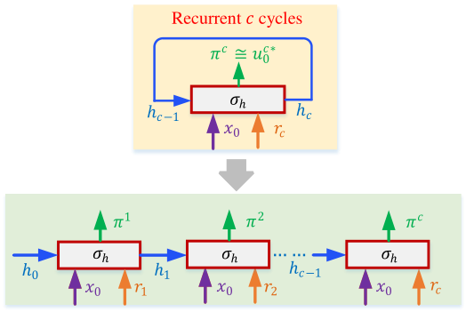
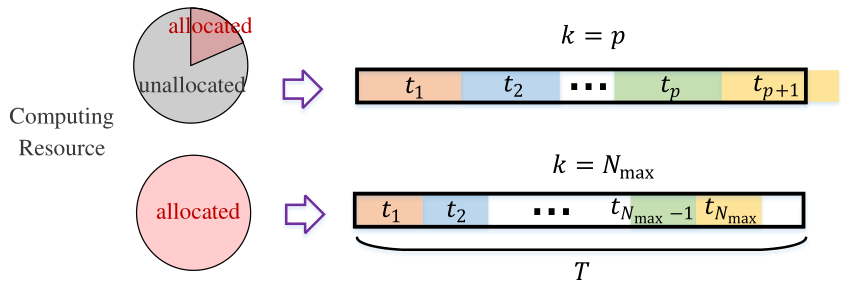
As shown in Fig. 1, the recurrent policy function calculates and outputs a control input at each recurrent cycle. Assuming that we have found the optimal parameters $\theta^{*}$, it follows that the output of the $c$th cycle $\pi^{c}(x_{0},r_{1:c};\theta^{*})={u^{c}_{0}}^{*}(x_{0},r_{1:c})$ for $\forall c\in[1,N_{\text{max}}]$. This indicates that the more cycles, the longer the prediction horizon. In practical applications, the calculation time of each cycle $t_{c}$ is different due to the dynamic change of computing resource allocation (see Fig. 2). At each time step, the total time assigned to the control input calculation is assumed to be $T$. Denoting the total number of the recurrent cycles at each time step as $k$, then the control input is $\pi^{k}(x_{0},r_{1:k};\theta^{*})$, where

Therefore, the recurrent policy is able to make full use of computing resources and adaptively select the longest prediction step $k$. In other word, the more computing resources allocated, the longer prediction horizon will be selected, which usually would lead to the better control performance.

To find the optimal parameters $\theta^{*}$ offline, we first need to represent the MPC cost function in (2) in terms of $\theta$, denoted by $V(x_{0},r_{1:N},N;\theta)$. From (2) and the Bellman’s principle of optimality, the global minimum $V^{*}(x_{0},r_{1:N},N)$ can be expressed as:

It follows that

Therefore, for the same $x_{0}$ and $r_{1:N}$, it is clear that

This indicates that the $i$th optimal control input ${u^{N}_{i-1}}^{*}(x_{0},r_{1:N})$ in (3) can be regarded as the optimal control input of the $N$-$i$+$1$-step MPC control problem with initial state $x_{i-1}$. Hence,by replacing all $u^{N}_{i-1}(x_{0},r_{1:N}))$ in (2) with $u^{N-i+1}_{0}(x_{i-1},r_{i:N})$, the $N$-step MPC control problem can also be solved via minimizing $V(x_{0},r_{1:N},N)=\sum_{i=1}^{N}l(x_{i},r_{i},u^{N-i+1}_{0}(x_{i-1},r_{i:N}))$. Then, we can obtain the $N$-step cost function in terms of $\theta$:

To find the optimal parameters $\theta^{*}$ that make (4) hold, we can construct the following objective function:

Therefore, we can update $\theta$ by directly minimizing $J(\theta)$. The policy update gradients can be derived as

where

Denoting $\pi^{N_{\text{max}}-i+1}(x_{i-1},r_{i:N_{\text{max}}};\theta)$ as $\pi^{N_{\text{max}}-i+1}$ and $l(x_{i},r_{i},\pi^{N_{\text{max}}-i+1}(x_{i-1},r_{i:N_{\text{max}}};\theta))$ as $l_{i}$, we have

By defining two immediate variables, $\phi_{i}=\frac{\mathrm{d}x_{i}}{\mathrm{d}\theta}$ and $\psi_{i}=\frac{\mathrm{d}\pi^{N_{\text{max}}-i+1}}{\mathrm{d}\theta}$, we have their recursive formula and the details of gradient backpropagation are shown in Fig.3.

Therefore, the gradient formula can be simplified as:

Taking the Gradient Descent (GD) method as an example, the updating rules of the policy function are

where $\alpha_{\theta}$ denotes the learning rate and $K$ indicates $K$th iteration.

The framework and pseudo-code of the proposed RMPC algorithm is shown in Algorithm 1 and Fig. 4.

There are many types of recurrent functions belonging to the structure defined in (5), and recurrent neural networks (RNN) are the most commonly used. In recent years, deep RNNs have been successfully implemented in many fields, such as natural language processing and system control, attributing to their ability to process sequential data [19, 20]. Next, we will show that as the iteration index $K\rightarrow\infty$, the optimal policy $\pi^{c}(x_{0},r_{1:c};\theta^{*})$ that make (4) hold can be achieved using Algorithm 1, as long as $\pi^{c}(x_{0},r_{1:c};\theta)$ is an over-parameterized RNN. The over-parameterization means that the number of hidden neurons is sufficiently large. Before the main theorem, the following lemma and assumption need to be introduced.

The reported experimental results and theoretical proofs have shown that the straightforward optimization methods, such as GD and Stochastic GD (SGD), can find global minima of most training objectives in polynomial time if the approximate function is an over-parameterized neural network or RNN [24, 25]. Based on this fact, we make the following assumption.

We now present our main result.

Thus, we have proven that RMPC algorithm can converge to $\theta^{*}$. In other words, it can find the nearly optimal policy of MPC with different prediction horizon, whose output after $c$th recurrent cycles corresponds to the nearly optimal solution of $c$-step MPC.

The policy network is trained offline on the PC, and then deployed to the industrial personal computer (IPC). The vehicle dynamics used for policy training are different from the controlled plant. For online applications, the IPveC-controller gives the control signal to the plant according to the state information and the reference trajectory. The plant feeds back the state information to the IPC-controller, so as to realize the closed-loop control process. The feedback scheme of the HIL experiment is depicted in Fig 5. The type of IPC-controller is ADLINK MXC-6401, equipped with Intel i7-6820EQ CPU and 8GB RAM, which is used as a vehicle on-board controller[28]. The plant is a real-time system, simulated by the vehicle dynamic model of CarSim [29]. The longitudinal speed is assumed to be constant, $v_{x}=16\text{m/s}$, and the expected trajectory is shown in Fig. 10. The system states and control inputs of this problem are listed in Table I, and the vehicle parameters are listed in Table II.

The offline policy is trained based on the nonliner and non input-affine vehicle dynamics:

where $F_{yf}$ and $F_{yr}$ are the lateral tire forces of the front and rear tires respectively [30]. The lateral tire forces can be approximated according to the Fiala tire model:

where $\alpha_{\#}$ is the tire slip angle, $F_{z\#}$ is the tire load, $\mu_{\#}$ is the friction coefficient, and the subscript $\#\in\{f,r\}$ represents the front or rear tires. The slip angles can be calculated from the relationship between the front/rear axle and the center of gravity (CG):

The loads on the front and rear tires can be approximated by:

The utility function of this problem is set to be $u_{i-1}$

Therefore, the policy optimization problem of this example can be formulated as:

where $V(x_{0},r_{1:{N_{\text{max}}}},{N_{\text{max}}};{\color[rgb]{1,0,0}\theta})=\sum_{i=1}^{N_{\text{max}}}l(x_{i},r_{i},u_{i-1})$, $u_{i-1}=\pi^{{N_{\text{max}}}-i+1}(x_{i-1},r_{i:{N_{\text{max}}}};\theta)$, $N_{\text{max}}=15$, $u_{\text{min}}=-0.2\text{rad}$ and $u_{\text{max}}=0.2\text{rad}$.

The policy function is represented by a variant of RNN, called GRU (Gated Recurrent Unit). The input layer is composed of the states, followed by 4 hidden layers using rectified linear unit (RELUs) as activation functions with $128$ units per layer, and the output layer is set as a $tanh$ layer, multiplied by $0.2$ to confront bounded control. We use Adam method to update the network with the learning rate of $2\times 10^{-4}$ and the batch size of $256$.

For nonlinear MPC problems, we can solve it with some optimization solvers, such as ipopt [17] and bonmin [18], which can be approximately regarded as the numerical optimal solution.

Fig. 6 compares the calculation efficiency of RMPC and the optimization solvers based on the symbolic framework CasADi [31] under different prediction steps for online applications. It is obvious that the calculation time of the optimization solvers is much longer than RMPC, and the gap increases with the number of prediction steps. Specifically, when $N=c=15$, the fastest optimization solver ipopt is over 5 times slower than RMPC (ipopt for $26.2$ms, RMPC for $4.7$ms). This demonstrates the effectiveness of the RMPC method.

We run Algorithm 1 for 10 times and calculate the policy error $e_{N}$ between the solution of ipopt solver and RMPC at each iteration for $N\in[1,15]$,

where ${{u^{N}_{\text{max}}}^{*}}$ and ${{u^{N}_{\text{min}}}^{*}}$ are respectively the maximum and minimum value of ${u_{0}^{N}}^{*}(x_{0},r_{1:N})$ for $\forall x_{0},r_{1:N}\in\mathcal{X}$, $\forall N\in[1,15]$, $N$ is the number of prediction steps. $e_{N}$ indicates the relative error of control quantity $\pi^{N}(\cdot)$ from cycle network respect to the optimum $u_{0}^{N^{*}}(\cdot)$ in $N$ step prediction control problem .

In Fig. 7, we plot policy error curves during training with different prediction steps $N$ . It is clear that all the policy errors decrease rapidly to a small value during the training process. In particular, after $10^{4}$ iterations, policy errors for all $N\geq 5$ reduce to less than 2%. This indicates that Algorithm 1 has the ability to find the near-optimal policy of MPC problems with different prediction horizons $N$.

Fig. 8 shows the policy performance of the ipopt solver solution and learned policy ${\pi^{c}}(x_{0},r_{1:c};\theta)$ with different prediction horizons. The policy performance is measured by the lost function of 200 steps (10s) during the simulation period staring from random initialized state, i.e.,

For all prediction domains $N$, the learned policy performs as well as the solution of ipopt solver. More recurrent cycles (or long prediction steps) help reduce the accumulated cost $L$.

In detail, Fig. 10 intuitively presents the control results of the learned policy with different recurrent cycles $c$ and Fig. 9 compares the control output between the learned policy(after 15 recurrent cycles) with ipopt controller.Obviously, the trajectory controlled by RMPC controller almost overlaps with the ipopt controller. The more recurrent cycles of the learned policy, the smaller the trajectory tracking error.This is why we want to adaptively select the optimal law with longest prediction horizon in real applications.

To summarize, the example demonstrates the optimality, efficiency and generality of the RMPC algorithm.

References

- [1] S. J. Qin and T. A. Badgwell, “A survey of industrial model predictive control technology,” Control engineering practice, vol. 11, no. 7, pp. 733–764, 2003.
- [2] S. Vazquez, J. Leon, L. Franquelo, J. Rodriguez, H. A. Young, A. Marquez, and P. Zanchetta, “Model predictive control: A review of its applications in power electronics,” IEEE Industrial Electronics Magazine, vol. 8, no. 1, pp. 16–31, 2014.
- [3] S. E. Li, Z. Jia, K. Li, and B. Cheng, “Fast online computation of a model predictive controller and its application to fuel economy–oriented adaptive cruise control,” IEEE Transactions on Intelligent Transportation Systems, vol. 16, no. 3, pp. 1199–1209, 2014.
- [4] J. H. Lee, “Model predictive control: Review of the three decades of development,” International Journal of Control, Automation and Systems, vol. 9, no. 3, p. 415, 2011.
- [5] R. Cagienard, P. Grieder, E. C. Kerrigan, and M. Morari, “Move blocking strategies in receding horizon control,” Journal of Process Control, vol. 17, no. 6, pp. 563–570, 2007.
- [6] Y. Wang and S. Boyd, “Fast model predictive control using online optimization,” IEEE Transactions on control systems technology, vol. 18, no. 2, pp. 267–278, 2009.
- [7] A. Bemporad, M. Morari, V. Dua, and E. N. Pistikopoulos, “The explicit linear quadratic regulator for constrained systems,” Automatica, vol. 38, no. 1, pp. 3–20, 2002.
- [8] B. Kouvaritakis, M. Cannon, and J. A. Rossiter, “Who needs qp for linear mpc anyway?” Automatica, vol. 38, no. 5, pp. 879–884, 2002.
- [9] T. Geyer, F. D. Torrisi, and M. Morari, “Optimal complexity reduction of polyhedral piecewise affine systems,” Automatica, vol. 44, no. 7, pp. 1728–1740, 2008.
- [10] C. N. Jones and M. Morari, “Polytopic approximation of explicit model predictive controllers,” IEEE Transactions on Automatic Control, vol. 55, no. 11, pp. 2542–2553, 2010.
- [11] C. Wen, X. Ma, and B. E. Ydstie, “Analytical expression of explicit mpc solution via lattice piecewise-affine function,” Automatica, vol. 45, no. 4, pp. 910–917, 2009.
- [12] F. Borrelli, M. Baotić, J. Pekar, and G. Stewart, “On the computation of linear model predictive control laws,” Automatica, vol. 46, no. 6, pp. 1035–1041, 2010.
- [13] B. M. Åkesson, H. T. Toivonen, J. B. Waller, and R. H. Nyström, “Neural network approximation of a nonlinear model predictive controller applied to a ph neutralization process,” Computers & chemical engineering, vol. 29, no. 2, pp. 323–335, 2005.
- [14] B. M. Åkesson and H. T. Toivonen, “A neural network model predictive controller,” Journal of Process Control, vol. 16, no. 9, pp. 937–946, 2006.
- [15] L. Cheng, W. Liu, Z.-G. Hou, J. Yu, and M. Tan, “Neural-network-based nonlinear model predictive control for piezoelectric actuators,” IEEE Transactions on Industrial Electronics, vol. 62, no. 12, pp. 7717–7727, 2015.
- [16] J. Duan, Z. Liu, S. E. Li, Q. Sun, Z. Jia, and B. Cheng, “Deep adaptive dynamic programming for nonaffine nonlinear optimal control problem with state constraints,” arXiv preprint arXiv:1911.11397, 2019.
- [17] A. Wachter and L. T. Biegler, “Biegler, l.t.: On the implementation of a primal-dual interior point filter line search algorithm for large-scale nonlinear programming. mathematical programming 106, 25-57,” Mathematical Programming, vol. 106, no. 1, pp. 25–57, 2006.
- [18] P. Bonami, L. T. Biegler, A. R. Conn, G. Cornuéjols, I. E. Grossmann, C. D. Laird, J. Lee, A. Lodi, F. Margot, N. Sawaya et al., “An algorithmic framework for convex mixed integer nonlinear programs,” Discrete Optimization, vol. 5, no. 2, pp. 186–204, 2008.
- [19] T. Mikolov, M. Karafiát, L. Burget, J. Černockỳ, and S. Khudanpur, “Recurrent neural network based language model,” in Eleventh annual conference of the international speech communication association, 2010.
- [20] S. Li, H. Wang, and M. U. Rafique, “A novel recurrent neural network for manipulator control with improved noise tolerance,” IEEE transactions on neural networks and learning systems, vol. 29, no. 5, pp. 1908–1918, 2017.
- [21] L. K. Li, “Approximation theory and recurrent networks,” in Proc. of IJCNN, vol. 2, pp. 266–271. IEEE, 1992.
- [22] A. M. Schäfer and H.-G. Zimmermann, “Recurrent neural networks are universal approximators,” International journal of neural systems, vol. 17, no. 04, pp. 253–263, 2007.
- [23] B. Hammer, “On the approximation capability of recurrent neural networks,” Neurocomputing, vol. 31, no. 1-4, pp. 107–123, 2000.
- [24] Z. Allen-Zhu, Y. Li, and Z. Song, “A convergence theory for deep learning via over-parameterization,” in International Conference on Machine Learning, pp. 242–252. Long Beach, California, USA: ICML, 2019.
- [25] S. Du, J. Lee, H. Li, L. Wang, and X. Zhai, “Gradient descent finds global minima of deep neural networks,” in International Conference on Machine Learning, pp. 1675–1685. Long Beach, California, USA: ICML, 2019.
- [26] Z. Allen-Zhu, Y. Li, and Z. Song, “On the convergence rate of training recurrent neural networks,” in Advances in Neural Information Processing Systems, pp. 6673–6685, 2019.
- [27] R. Li, Y. Li, S. E. Li, E. Burdet, and B. Cheng, “Driver-automation indirect shared control of highly automated vehicles with intention-aware authority transition,” in 2017 IEEE Intelligent Vehicles Symposium (IV), pp. 26–32. Redondo Beach, California, USA: IEEE, 2017.
- [28] C. Chen, J. Pan, X. Chang, Q. Xu, and J. Wang, “System design and function verification of an extensible autonomous driving platform,” in 2019 IEEE International Symposium on Circuits and Systems (ISCAS), pp. 1–5. Sapporo, Japan: IEEE, 2019.
- [29] R. Benekohal and J. Treiterer, “Carsim: Car-following model for simulation of traffic in normal and stop-and-go conditions,” Transportation research record, vol. 1194, pp. 99–111, 1988. [Online]. Available: http://dx.doi.org/
- [30] J. Kong, M. Pfeiffer, G. Schildbach, and F. Borrelli, “Kinematic and dynamic vehicle models for autonomous driving control design,” in 2015 IEEE Intelligent Vehicles Symposium (IV), pp. 1094–1099. Seoul, South Korea: IEEE, 2015.
- [31] J. A. E. Andersson, G. Joris, H. Greg, J. B. Rawlings, and D. Moritz, “Casadi: a software framework for nonlinear optimization and optimal control,” Mathematical Programming Computation, vol. 11, pp. 1–36, 2018.