Inflation and Scale-invariant –Gravity
Abstract
In scale–invariant models of fundamental physics, mass scales are generated by spontaneous symmetry breaking. In this work, we study inflation in scale-invariant gravity, in which the Planck mass is generated by a scalar field, which is responsible for spontaneous breaking of scale–symmetry. If the self–interactions of the scalar field are non-zero, a cosmological constant is generated, which can be potentially quite large. To avoid fine–tuning at late times, we introduce another scalar field which drives the classical cosmological constant to zero during inflation. Working in the Einstein–frame, we find that due to a conserved Noether current the corresponding three–field inflationary model (consisting of the two scalar fields plus the scalaron) becomes effectively a two–field model. The prize to be paid for introducing the field which cancels the classical cosmological constant at the end of inflation is that the running of the spectral index and the running of the running can be quite large due to entropy perturbations during inflation, making the model testable with future cosmological experiments.
pacs
Valid PACS appear hereI Introduction
Cosmological inflation, a short period of accelerated expansion in the very early universe, is a simple and powerful idea Guth 1981; Starobinsky 1987; Albrecht and Steinhardt 1982; Linde 1982. It provides an explanation for the current homogeneity and isotropy of our universe and suggests that the origins of the observed structures are results from quantum processes in the very early universe Mukhanov and Chibisov 1981; Hawking 1982; Bardeen et al. 1983; Liddle and Lyth 2000; Baumann 2011; Riotto 2010. Predictions from inflation, such as the spectral index and the tensor-to-scalar ratio, fit observations such as those from the Planck experiment very well Akrami et al. 2020; Chowdhury et al. 2019. Nevertheless, despite its appeal and simplicity, embedding inflation in fundamental theories of physics remains a challenge. On top of this, current observations indicate that the universe undergoes an epoch of accelerated expansion at the present time too. Both energy scales differ by many orders of magnitude. Finding an explanation from particle physics or theories of gravity for each epoch of accelerated expansion remains an active field of research.
Inflation might be driven due to new matter sectors in a fundamental theory, or due to modifications of the gravitational sector or both Martin et al. 2014. Among the popular inflationary models, Starobinsky’s original model of inflation, based on an additional –term in the gravitational sector Starobinsky 1987, and its variants are promising models. There is considerable hope that modifications to General Relativity (GR) appear naturally in fundamental theories. From the phenomenological side, there have been many works studying the –model and its extensions, see Edery and Nakayama 2019; Gottlober et al. 1991; Rinaldi and Vanzo 2016; Tambalo and Rinaldi 2017; Bamba et al. 2015; Antoniadis et al. 2020; Calmet and Kuntz 2016; Capozziello et al. 2006; De Felice and Tsujikawa 2010; Tang and Wu 2020; van de Bruck and Paduraru 2015; Ferreira et al. 2019. In this paper we consider an extension of –gravity, in which there is no intrinsic mass scale, i.e. it is scale–invariant. The Planck mass, specified by the vacuum expectation value of a fundamental scalar field, is dynamically generated during inflation, similar to models studied in Rinaldi and Vanzo 2016; Tambalo and Rinaldi 2017; Ferreira et al. 2016; Ferreira et al. 2017; Ferreira et al. 2019; Kubo et al. 2019; Kubo et al. 2020. As it was shown in earlier work Rinaldi and Vanzo 2016; Tambalo and Rinaldi 2017; Ferreira et al. 2019, and as we will review in Section 2, the prediction of the model for the spectral index and the tensor-to-scalar ratio are equivalent to the original Starobinsky model. However, as we will emphasise in Section 2, a classical cosmological constant is generated after inflation, which can be potentially large, unless the self–interaction of the scalar field is unnaturally small or zero if the classical cosmological constant is tuned to be zero. In this paper we extend the model by introducing another scalar field which dynamically drives the cosmological constant to zero during inflation. As we will show, the dynamics of this second field will generate features in the primordial power spectrum and a cut-off at small wavelength. After inflation, the theory is well approximated by GR with vanishing classical cosmological constant. The scalaron field, describing modifications from GR due to the term, is heavy and has therefore a very small interaction range.
The paper is organized as follows. In Section II we discuss the prediction of scale invariant inflation, which in the Einstein frame is a two–field model. We recover the results of previous work, highlighting the fact that the theory predicts a large cosmological constant in the Einstein frame unless the field determining the Planck mass has no self-interactions. In Section III we present a modification by adding another scalar field, whose role is to cancel the cosmological constant. In the Einstein frame, the theory is described by a three–field system. The inflationary dynamics and results from the numerical computations are discussed in Section IV. Our conclusions can be found in Section V. In the appendix we present the perturbation equations and describe an extension of Gordon et al. 2000; Lalak et al. 2007 in performing a field rotation into adiabatic and entropy fields for a three–field inflationary system and also discuss the numerical setup.
II A two-field model
The scale–independent models we study in this paper are extensions of Starobinsky’s -model Starobinsky 1987, in which there is no intrinsic mass scale. Instead, the Planck mass is generated dynamically during inflation. In this Section we will consider one additional scalar field to the model, which couples to the Ricci–scalar. The action is specified by
| (1) |
with
| (2) | |||||
| (3) |
Here, and are constant parameter. This set-up has previously been studied in the context of inflation in Tambalo and Rinaldi 2017; Ferreira et al. 2019. We will recover some of the results of the literature in the following, emphasising the fact that the cosmological constant at the end of inflation is non-zero and potentially quite large unless or unnaturally small.
To analyse the predictions from inflation, we will study the model in the Einstein–frame. Theories of the –type can be brought into the Einstein–frame via a conformal transformation of the metric (see Hwang 1997; Rodrigues et al. 2011 and e.g. De Felice and Tsujikawa 2010 and references therein). Defining the auxiliary field with and considering the conformal transformation , the action can be brought into the Einstein frame, which takes the form
| (4) |
where we identify . The total potential energy for our model will be specified below. Note that sets an arbitrary mass-scale, which we have identified with the Planck mass in the Einstein frame.
Theories of the form (4) have been considered in e.g. Di Marco et al. 2003; Lalak et al. 2007; van de Bruck and Robinson 2014; van de Bruck and Paduraru 2015; van de Bruck and Longden 2016. For the –model we are considering in this paper, specified by equations (2) and (3), we have
| (5) |
At the minimum of the potential, specified by , we find
| (6) |
The potential energy at the minimum is given by
| (7) |
Thus, as long as does not vanish, a cosmological constant is generated11 1 In the Jordan–frame, after inflation the vacuum expectation value of does not vanish. The potential energy will not vanish either if is non-zero, resulting in a positive cosmological constant.. Furthermore, we can calculate the mass of the scalaron at the minimum. We find
| (8) |
Therefore, in this model the cosmological constant and the scalaron mass are linked via
| (9) |
The Jordan–frame action (1)-(3) is invariant under the global Weyl transformation
| (10) |
In the Einstein frame, with the action given by (4) and the potential energy given by (5), there exists a corresponding symmetry as well: the field–transformation
| (11) |
leaves the Einstein–frame action invariant. As a result, the following current is conserved
| (12) |
i.e.
| (13) |
Considering a flat Robertson–Walker metric with
where is the scale factor, this equation implies that, in cosmology,
| (14) |
Therefore, during inflation in which the scale factor grows quasi–exponentially, we quickly approach a regime where
| (15) |
and the two–field model quickly becomes effectively a one–field system. This allows us to rewrite eq. (5) as
| (16) |
which is the effective potential during inflation at sufficient late times.
We now turn to find the constraints on the parameter of the model. Apart from constraints coming from the spectral index, the tensor-to-scalar ratio and the amplitude of scalar perturbations generated during inflation, we will discuss the implications of the non–vanishing vacuum energy density in the model too.
To analyse the evolution of the fields during inflation, we state the slow-roll parameters of our model
| (17) |
| (18) |
We have a successful slow-roll inflationary period while , which sets the field value at the end of inflation to be From the slow roll parameters we determine the inflationary observables, the scalar spectral index, and the tensor-to-scalar ratio, , from the background fields,
| (19) |
Here we have written and in terms of the number of e-folds, , to highlight the fact that the prediction for these observables are the same as in Starobinsky inflation. We will assume that the horizon crossing is at . We can then finally begin to constrain the model parameters from the energy scale of inflation, . In our model we use the form of (16) which gives
| (20) |
The interaction range of the scalaron is less than a millimeter, implying that . This allows us to further constrain our model via (8) to give
| (21) |
Finally, we demand that the energy density at the minimum drives the cosmological expansion today, i.e. we set at the minimum to be the observed dark energy density. This gives the result
| (22) |
This result implies that has to be unnaturally small, coming from the demand that the cosmological constant is small. Of course, dark energy might originate from a different sector in the theory and we could simply demand that . On the other hand, rather than relying on the self–interactions to vanish or to be unnaturally small, it would be more satisfying if the (classical) cosmological constant is dynamically driven to zero during inflation. In the next section we discuss a model in which exactly this happens. To achieve this, we employ another scalar field.
III A three–field model
The action we consider is a variant of the action (1), with the addition of a second field :
| (23) |
with
| (24) | |||||
| (25) |
Here we couple only to the Ricci–scalar and only determines the value of the Planck mass. An extension of the model in which also the –field couples to the Ricci–scalar is possible, but that would introduce another parameter. The role of the field is to drive the cosmological constant in the Einstein–frame to zero.
In the Einstein frame the action becomes a three-field system and reads
| (26) |
with the potential
| (27) |
With the addition of the new field, the potential has now a global minimum at which . This is similar to a dynamical Higgs VEV model shown in Garcia-Bellido et al. 2011. At the minimum we have
| (28) |
As a consequence, is now only constrained by the amplitude of primordial scalar perturbations.
The equations of motions for the fields in our model are given by
| (29) | ||||
| (30) | ||||
| (31) |
In an expanding homogeneous and isotropic universe, the Friedmann equation reads
| (32) |
The action is invariant under the following transformations of the fields
and as before there is a conserved current, which allows us to reduce our system to an effective two field case at late times during inflation. Following a calculation similar to the two-field case, we find that at late times
| (33) |
where is a constant of integration, specified by initial conditions for the fields. This has been confirmed numerically with various initial conditions and parameters. We will use this result in the next section to simplify and understand the results of our model.
IV Background evolution and cosmological perturbations


Since the three-field system is too complicated to find useful analytical solutions, we study the inflationary dynamics and the evolution of perturbations numerically. The evolution of the fields is governed by the following set of (background) equations:
| (34) | |||||
| (35) | |||||
| (36) |
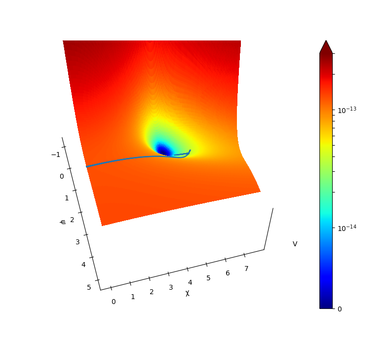
During inflation, the Noether current implies that eq. (33) is fulfilled after a few e-folds. Using this equation to relate to and and plugging this into the potential , we obtain an effective two–field potential. The precise form of this effective two-field potential depends on the initial conditions for the fields, encoded in the constant in eq. (33), but there are some general features, as seen in fig. 1: in the –direction we have plateau-like potential with a barrier near , typical for theories. However, the addition of creates a well in the potential. At the bottom of the well the potential energy vanishes.
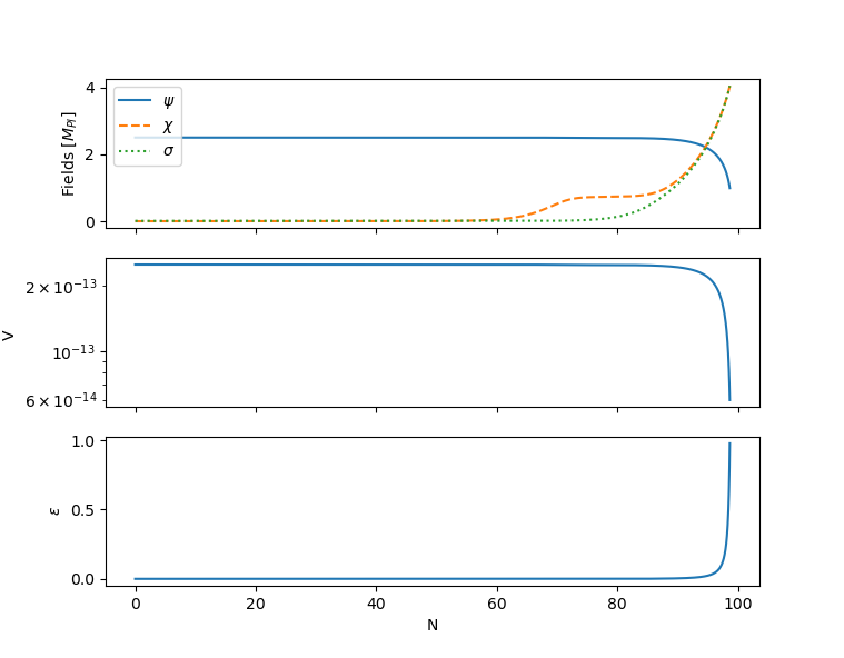
The dynamics of the fields depends on the initial conditions. Here, we concentrate at the case and . In the first part of inflation is effectively frozen, whereas and rolling down the potential. This is a similar behaviour to that of multifield -attractor models Linde et al. 2018. The fields settle in a local valley (shown in fig. 1) at which point the slow–roll conditions are briefly violated, as it can be seen from the evolution of the slow-roll parameter in fig. 2. In fact the condition is severely violated at this point, creating additional features in the power spectrum as we will see later. From this point onward, the field is effectively frozen. However, continues to roll slowly, influenced by its coupling to . The field evolves during this time too. Eventually catches up with forcing the fields to fall into the global minimum, driving the potential to zero and ending inflation. The final values of , and are dictated by the initial conditions.
To analyse the resulting power spectra, we have varied each of the parameters , and individually in fig. 3, while keeping the initial conditions for the fields fixed. We will summarize our findings in the following and refer to the Appendix appendix A for the details on the numerical procedure. In the Appendix we also derive the perturbations of the adiabatic and entropy fields for a generic three-field system as studied in this paper. From our numerical calculations we find that determines the range of –values for which the power spectrum of scalar perturbations is nearly scale–independent. This is because determines the width of the valley region in the potential. A small parameter results in an earlier start of the second period of inflation (for a given set of initial conditions). On the other hand, determines the steepness of the potential into the valley region, with smaller decreasing the gradient. Finally, determines the potential energy within the valley, as it can be seen from eq. 27. The parameter and affect the transition to the second period of inflation and therefore affect the spike in the evolution of epsilon. As such they have a large effect on the amplitude of the power spectrum for wave numbers which leave the horizon around the transition from the first to the second period of inflation.
As mentioned, initially is effectively frozen, as illustrated in fig. 2. For the initial conditions used here, the initial value of is small but the initial value of is smaller. Because the potential gradient in the –direction is smaller than in the –direction, the value of will eventually become larger than , creating a brief period of strong interactions between the two fields at that time. This causes to oscillate as it rolls, which can be seen from the evolution of in fig. 2. We find that while is small initially, the second slow roll parameter becomes large during this time, as shown in fig. 2. Eventually, after about 22 e-folds the fields settle and slow–roll inflation begins (both and ) and this (first) period of inflation last for over 50 e-folds. The drop in amplitude in fig. 3 at large scales which we observe in some runs for some choice of parameter is due to the fact that those scales cross the Hubble radius during this initial period in which becomes large. In the case of initial conditions where , the violation of the slow–roll condition does not occur and there is no drop in amplitude of power at small –values.
Once the slow–roll parameter are small during the first period of inflation the produced power spectrum is approximately flat, as expected. The three fields evolve only very slowly during this period. In our numerical runs, we have chosen the parameter such that the amplitude of the scalar perturbations match data from the CMB. For large –values we see a drop in the power spectrum, caused by the end of the second period of inflation as the fields fall into the global minimum of the potential. The –field is evolving considerably during the second period of inflation. This in turn forces the fields into a steep potential, increasing the velocity of the fields. This drop of power at small scales means our model does not predict the formation of primordial black holes. Unlike similar models to ours, our potential does not create a large entropy perturbations, we actually see the opposite effect due to the evolution of from zero (this effect has been studied in similar models to ours in Gundhi and Steinwachs 2020 and Gundhi et al. 2020).
The predicted power spectra are not well described by a power law. Even if we allow for a running of the spectral index and a running of the running , the usual approximation for the power spectrum
where both and are evaluated at the pivot point , is not a good one as both and csn vary substantially as a function of wave-number in the model discussed. From our numerical simulations we find that the predicted tensor-to-scalar ratio is of order , substantially reduced to the two field case discussed in Section 2 (and see Ferreira et al. 2019). Other scale invariant models find a similar reduction in , see e.g. Antoniadis et al. 2020Gialamas et al. 2020. For the parameters values , , and , we find that the spectral index is consistent with current CMB observations, , and has a substantial running () at large scales but varies widely and becomes negative at large wavenumbers. The running of the running is and roughly of similar order of magnitude as the running (but negative for all values of ). The model is an example in which isocurvature modes can cause the running of the spectral index and the running of the running to be of similar order of magnitude van de Bruck and Longden 2016. We expect this model to be tightly constrained by current observations, but we leave this analysis for future work.

Finally we look at how the features alter the predictions of the CMB angular spectra. In fig. 3 is clear that a change of or corresponds to a change in curvature’s amplitude. As such, we have constrained the value of and to fix with . We then computed the CMB temperature angular spectra using CAMB Lewis et al. 2000. We see that the features naturally manifest themselves at lower multipoles. However, even a small change in causes a shift in the amplitude of the power spectrum corresponding to a shift in amplitude in fig. 4.


So far we have concentrated on the case . To understand the parameter space of our model better, we briefly discuss the case . A typical form of the potential is shown in fig. 5. We can see that this results in an effective single period of inflation with two fields, as and become equal well before the end of inflation, tracing each others trajectory illustrated in fig. 5. There is almost a hint of another local minimum, within the potential tench of fig. 5. However, the fields will not settle here, as it can be seen from the trajectory. The resulting power spectrum is also shown in fig. 5. For the parameter chosen is does not fit the data at all, but we find generally that the flat part of the spectrum does not range over many orders of magnitude in –values. The case will be even more constrained than the case .
V Discussion and conclusions
We have studied the scale invariant extension of inflation introduced in Tambalo and Rinaldi 2017; Ferreira et al. 2019, pointing out that while it is a successful inflationary model, a non-zero cosmological constant is generated due to the self-coupling of the scalar field , whose VEV generates the Planck mass. To remove the potentially large cosmological constant at the end of inflation, we extend the model and add another scalar field , with interacts with in a scale–invariant way, forcing the vacuum energy to vanish at the global minimum.
We analyse the system in the Einstein frame, in which inflation is driven by three scalar fields ( and the scalaron ). To calculate the power spectra for scalar and tensor perturbations, we extended the two–field formalism of Gordon et al. 2000 and Lalak et al. 2007 to three fields. We used a similar methodology, creating two orthogonal components (equivalent to the entropy components), with respect to the tangential/trajectory direction in field space (corresponding to the curvature component, the details can be found in the Appendix).
Our results show that the model can exhibit two periods of inflation. The two periods are separated by a brief (and mild) violation of the smallness of the slow roll parameter. We have numerically solved the perturbation equations and determine the power spectrum for different parameter. From the amplitude of CMB anisotropies we find that small values for the parameter are preferred (). We identify three regimes in the predicted scalar power spectrum: at large scales, where the scales cross the horizon before all three fields begin to slow roll, the power decreases due to violation of the smallness of the parameter; at intermediate scales the power spectrum is flat and can match the CMB data; and at large wavenumber we find a further decrease in the amplitude for very large –values (the scales leave the horizon in the second period of inflation, at the time when rolls significantly and is driving the potential to zero and eventually ending inflation).
We also discussed the predictions for the spectral index , its running , the running of the running and the tensor–to–scalar ratio . We see a substantial reduction in compared to ordinary –inflation and its scale–invariant version of Tambalo and Rinaldi 2017; Ferreira et al. 2019. We find that the model can potentially break the usual hierarchy , due to entropy perturbations produced by the field, making the model testable with current and future cosmological data.
It will be interesting to study reheating and preheating in this model, given that the three fields are all coupled together. Another direction to take is to analyse this model further by studying a variety of initial conditions for the fields and constraining the model parameter with current cosmological data.
Acknowledgements.
CvdB is supported (in part) by the Lancaster–Manchester–Sheffield Consortium for Fundamental Physics under STFC grant: ST/T001038/1. RD is supported by a STFC studentship.Appendix A Three field numerical procedure
A.1 Linear Perturbations
In this Appendix we derive the linear perturbation equations for the theory presented in Section III. We shall be following the work of Gordon et al. 2000, Di Marco et al. 2003 and Lalak et al. 2007 for the two field case and extending it to three fields. Detailed literature on the theory of cosmological perturbation can be found Mukhanov et al. 1992. Working in the longitudinal gauge and with the absence of the anistropic stress, the metric is
| (37) |
where is the metric perturbation in this gauge. The fields are broken down into background and perturbations parts,
| (38) |
This allows us to find the perturbed Klein-Gordon equations (we define to match the notation in the literature Di Marco et al. 2003)
| (39) |
| (40) |
| (41) |
The right hand side of the perturbed Klein-Gordon contain the metric perturbation, which is subject to the perturbed Einstein equations Mukhanov et al. 1992
| (42) |
| (43) |
We define the gauge invariant Mukhanov-Sasaki variables to further study the evolution of the perturbations,
| (44) |
Using (42) and (43), this allows us to rewrite our perturbed Klein-Gordon equations (39) - (41) as
| (45) |
| (46) |
| (47) |
with the coefficients
Due to the symmetry between and , as expected the perturbed Klein-Gordon equations also carry this symmetry. For brevity, we have labelled the coefficients with , where and is the other field.
A.2 Tangential and normal perturbations
For multifield inflation we break down the perturbations into tangential and normal components with respect to the trajectory of the perturbations, first introduced in Gordon et al. 2000 and extended to nonlinear perturbations in Langlois and Vernizzi 2007. The tangential perturbation equates to the curvature or adiabatic component while the normal perturbations are the entropy components. As described in Peterson and Tegmark 2013 we have one curvature component and entropy components, where is the number of effective fields.
We define the curvature perturbation in the standard way Mukhanov et al. 1992
| (48) |
For our case we find
| (49) |
Here, is the three field adiabatic component, representing the velocity parallel to the trajectory. This allows us to define as the instantaneous curvature Mukhanov-Sasaki variable corresponding to the perturbations parallel to the trajectory , defined in the same way as Gordon et al. 2000. Following the methodology laid out in Lalak et al. 2007, we set up our three field model by extending the 2D circular coordinate system to a 3D spherical system, using as an effective radial component,
| (50) |
After equating coefficients and some basic algebra we determine,
| (51) |
Now with our angles established we can calculate the entropy perturbations, and , which are defined to be orthogonal to the trajectory, :
| (52) |
Using (51) we can rewrite this in terms of the fields,
| (53) |
We can then calculate the entropy component as . More importantly, we now have a complete system for our three field system that allows us to relate our field perturbations into tangential and normal components via the rotational matrix,
| (54) |
Finally, we can determine how the curvature component is sourced. To do this, and for completion, we find the Klein-Gordon equation for our adiabatic field,
| (55) |
and the turning rate,
| (56) |
The adiabatic and entropy potentials follow the same rotation as (54),
| (57) |
Taking the derivative of with respect to time we find a nice compact version, similar to that of Gordon et al. 2000, Di Marco et al. 2003, and Braglia et al. 2020
| (58) |
In the derivation, we have used the comoving energy density found from the energy and momentum constraints ((42) and (43)),
| (59) |
A.3 Numerical setup
For the numerical calculations, we work with the more convenient time variable (the number of e-folds, defined by ) rather than cosmic time. We also set the pivot scale to leave the Hubble radius 50 e-folds before the end of inflation. We impose Bunch-Davis initial conditions (BD) on our tangential and normal perturbations (), separately, and deep inside the Hubble radius. To do this, we integrate (45)-(47), with the initial conditions,
| (60) |
To confirm that integration starts deep inside the Hubble radius, we impose these initial conditions when .
To ensure that there is no correlation between the curvature and entropy modes deep inside the Hubble radius, we integrate the perturbation equations three times, with different initial conditions. In the first run, we choose to have BD initial conditions and ; then we permute these initial conditions on each of the components. We indicate the run by roman numerals, so that the results of each run are , and and correspondingly for and . This will then allow us to compute the curvature and isocurvature power spectrum from our three runs and obtain the prediction for the power spectra as follows:
| (61) |
| (62) |
| (63) |
We compute the tensor power spectrum as follows (see e.g. Riotto 2010): The mode equation for gravitational waves is given by
| (64) |
where ′ denotes the derivative with respect to conformal time. The power spectrum is then given by
| (65) |
References
- Guth (1981) A. H. Guth, Phys. Rev. D 23, 347 (1981).
- Starobinsky (1987) A. A. Starobinsky, Adv. Ser. Astrophys. Cosmol. 3, 130 (1987).
- Albrecht and Steinhardt (1982) A. Albrecht and P. J. Steinhardt, Phys. Rev. Lett. 48, 1220 (1982).
- Linde (1982) A. D. Linde, Phys. Lett. B 108, 389 (1982).
- Mukhanov and Chibisov (1981) V. F. Mukhanov and G. V. Chibisov, JETP Lett. 33, 532 (1981).
- Hawking (1982) S. W. Hawking, Phys. Lett. B 115, 295 (1982).
- Bardeen et al. (1983) J. M. Bardeen, P. J. Steinhardt, and M. S. Turner, Phys. Rev. D 28, 679 (1983).
- Liddle and Lyth (2000) A. R. Liddle and D. H. Lyth, Cosmological inflation and large scale structure (2000).
- Baumann (2011) D. Baumann, in Theoretical Advanced Study Institute in Elementary Particle Physics: Physics of the Large and the Small (2011) pp. 523–686, arXiv:0907.5424 [hep-th] .
- Riotto (2010) A. Riotto, in 5th CERN - Latin American School of High-Energy Physics (2010) arXiv:1010.2642 [hep-ph] .
- Akrami et al. (2020) Y. Akrami et al. (Planck), Astron. Astrophys. 641, A10 (2020), arXiv:1807.06211 [astro-ph.CO] .
- Chowdhury et al. (2019) D. Chowdhury, J. Martin, C. Ringeval, and V. Vennin, Phys. Rev. D 100, 083537 (2019), arXiv:1902.03951 [astro-ph.CO] .
- Martin et al. (2014) J. Martin, C. Ringeval, and V. Vennin, Phys. Dark Univ. 5-6, 75 (2014), arXiv:1303.3787 [astro-ph.CO] .
- Edery and Nakayama (2019) A. Edery and Y. Nakayama, JHEP 11, 169 (2019), arXiv:1908.08778 [hep-th] .
- Gottlober et al. (1991) S. Gottlober, V. Muller, and A. A. Starobinsky, Phys. Rev. D 43, 2510 (1991).
- Rinaldi and Vanzo (2016) M. Rinaldi and L. Vanzo, Phys. Rev. D 94, 024009 (2016), arXiv:1512.07186 [gr-qc] .
- Tambalo and Rinaldi (2017) G. Tambalo and M. Rinaldi, Gen. Rel. Grav. 49, 52 (2017), arXiv:1610.06478 [gr-qc] .
- Bamba et al. (2015) K. Bamba, S. D. Odintsov, and P. V. Tretyakov, Eur. Phys. J. C 75, 344 (2015), arXiv:1505.00854 [hep-th] .
- Antoniadis et al. (2020) I. Antoniadis, A. Karam, A. Lykkas, T. Pappas, and K. Tamvakis, PoS CORFU2019, 073 (2020), arXiv:1912.12757 [gr-qc] .
- Calmet and Kuntz (2016) X. Calmet and I. Kuntz, Eur. Phys. J. C 76, 289 (2016), arXiv:1605.02236 [hep-th] .
- Capozziello et al. (2006) S. Capozziello, S. Nojiri, S. D. Odintsov, and A. Troisi, Phys. Lett. B 639, 135 (2006), arXiv:astro-ph/0604431 .
- De Felice and Tsujikawa (2010) A. De Felice and S. Tsujikawa, Living Rev. Rel. 13, 3 (2010), arXiv:1002.4928 [gr-qc] .
- Tang and Wu (2020) Y. Tang and Y.-L. Wu, Phys. Lett. B 809, 135716 (2020), arXiv:2006.02811 [hep-ph] .
- van de Bruck and Paduraru (2015) C. van de Bruck and L. E. Paduraru, Phys. Rev. D 92, 083513 (2015), arXiv:1505.01727 [hep-th] .
- Ferreira et al. (2019) P. G. Ferreira, C. T. Hill, J. Noller, and G. G. Ross, Phys. Rev. D 100, 123516 (2019), arXiv:1906.03415 [gr-qc] .
- Ferreira et al. (2016) P. G. Ferreira, C. T. Hill, and G. G. Ross, Phys. Lett. B 763, 174 (2016), arXiv:1603.05983 [hep-th] .
- Ferreira et al. (2017) P. G. Ferreira, C. T. Hill, and G. G. Ross, Phys. Rev. D 95, 064038 (2017), arXiv:1612.03157 [gr-qc] .
- Kubo et al. (2019) J. Kubo, M. Lindner, K. Schmitz, and M. Yamada, Phys. Rev. D 100, 015037 (2019), arXiv:1811.05950 [hep-ph] .
- Kubo et al. (2020) J. Kubo, J. Kuntz, M. Lindner, J. Rezacek, P. Saake, and A. Trautner, (2020), arXiv:2012.09706 [hep-ph] .
- Gordon et al. (2000) C. Gordon, D. Wands, B. A. Bassett, and R. Maartens, Phys. Rev. D 63, 023506 (2000), arXiv:astro-ph/0009131 .
- Lalak et al. (2007) Z. Lalak, D. Langlois, S. Pokorski, and K. Turzynski, JCAP 07, 014 (2007), arXiv:0704.0212 [hep-th] .
- Hwang (1997) J.-c. Hwang, Class. Quant. Grav. 14, 1981 (1997), arXiv:gr-qc/9605024 .
- Rodrigues et al. (2011) D. C. Rodrigues, F. de O. Salles, I. L. Shapiro, and A. A. Starobinsky, Phys. Rev. D 83, 084028 (2011), arXiv:1101.5028 [gr-qc] .
- Di Marco et al. (2003) F. Di Marco, F. Finelli, and R. Brandenberger, Phys. Rev. D 67, 063512 (2003), arXiv:astro-ph/0211276 .
- van de Bruck and Robinson (2014) C. van de Bruck and M. Robinson, JCAP 08, 024 (2014), arXiv:1404.7806 [astro-ph.CO] .
- van de Bruck and Longden (2016) C. van de Bruck and C. Longden, Phys. Rev. D 94, 021301 (2016), arXiv:1606.02176 [astro-ph.CO] .
- Garcia-Bellido et al. (2011) J. Garcia-Bellido, J. Rubio, M. Shaposhnikov, and D. Zenhausern, Phys. Rev. D 84, 123504 (2011), arXiv:1107.2163 [hep-ph] .
- Linde et al. (2018) A. Linde, D.-G. Wang, Y. Welling, Y. Yamada, and A. Achúcarro, JCAP 07, 035 (2018), arXiv:1803.09911 [hep-th] .
- Gundhi and Steinwachs (2020) A. Gundhi and C. F. Steinwachs, Nucl. Phys. B 954, 114989 (2020), arXiv:1810.10546 [hep-th] .
- Gundhi et al. (2020) A. Gundhi, S. V. Ketov, and C. F. Steinwachs, (2020), arXiv:2011.05999 [hep-th] .
- Gialamas et al. (2020) I. D. Gialamas, A. Karam, and A. Racioppi, JCAP 11, 014 (2020), arXiv:2006.09124 [gr-qc] .
- Lewis et al. (2000) A. Lewis, A. Challinor, and A. Lasenby, Astrophys. J. 538, 473 (2000), https://camb.info, arXiv:astro-ph/9911177 .
- Mukhanov et al. (1992) V. Mukhanov, H. Feldman, and R. Brandenberger, Physics Reports 215, 203 (1992).
- Langlois and Vernizzi (2007) D. Langlois and F. Vernizzi, JCAP 02, 017 (2007), arXiv:astro-ph/0610064 .
- Peterson and Tegmark (2013) C. M. Peterson and M. Tegmark, Phys. Rev. D 87, 103507 (2013), arXiv:1111.0927 [astro-ph.CO] .
- Braglia et al. (2020) M. Braglia, D. K. Hazra, F. Finelli, G. F. Smoot, L. Sriramkumar, and A. A. Starobinsky, JCAP 08, 001 (2020), arXiv:2005.02895 [astro-ph.CO] .