Quantum detector tomography of a high dynamic-range superconducting nanowire single-photon detector

Timon Schapeler Email: timon.schapeler@upb.de Address: Mesoscopic Quantum Optics, Paderborn University, Warburger Straße 100, 33098 Paderborn, Germany Jan Philipp Höpker Address: Mesoscopic Quantum Optics, Paderborn University, Warburger Straße 100, 33098 Paderborn, Germany Tim J. Bartley Address: Mesoscopic Quantum Optics, Paderborn University, Warburger Straße 100, 33098 Paderborn, Germany

Abstract

We demonstrate and verify quantum detector tomography of a superconducting nanowire single-photon detector (SNSPD) in a multiplexing scheme which permits measurement of up to 71000 photons per input pulse. We reconstruct the positive operator valued measure (POVM) of this device in the low photon-number regime, and use the extracted parameters to show the POVMs spanning the whole dynamic range of the device. We verify this by finding the mean photon number of a bright state. Our work shows that a reliable quantum description of large-scale SNSPD devices is possible, and should be applicable to other multiplexing configurations.

I Introduction

Since their invention at the turn of the century Gol’Tsman et al. 2001, superconducting nanowire single-photon detectors (SNSPDs) have become ubiquitous in quantum optics experiments, due to their low noise, high speed and high efficiency Natarajan et al. 2012; Marsili et al. 2013; Shibata et al. 2015; Esmaeil Zadeh et al. 2017; Korzh et al. 2020. Although recent work has shown that some photon number resolution can be recovered directly from the output of the detector by modifying the bias circuitry Cahall et al. 2017; Zhu et al. 2018; Zhu et al. 2020; Zou et al. 2020, in standard operation, however, these detectors do not resolve the number of photons incident. To overcome this, SNSPDs can be multiplexed in arrays, either spatial Dauler et al. 2007; Divochiy et al. 2008; Marsili et al. 2009; Jahanmirinejad et al. 2012; Zhao et al. 2013; Rosenberg et al. 2013; Verma et al. 2014; Miki et al. 2014; Allman et al. 2015; Shaw et al. 2015; Najafi et al. 2015; Chen et al. 2019; Tao et al. 2019; Wollman et al. 2019 or temporal Natarajan et al. 2013; Tiedau et al. 2019; Jönsson et al. 2020, such that the number of pixels in the array that fire gives some information about the number of photons that were incident.

The exact nature of the response of the device to different numbers of incident photons can be formally reconstructed using quantum detector tomography Lundeen et al. 2009. This techniques provides a fully quantum mechanical description of the operation of the device, without relying on any underlying physical model of its detection mechanism. This allows one to state the probability that a specific number of photons were incident, given a particular detector outcome, know as a positive operator valued measure (POVM). Quantum detector tomography has been carried out for single-pixel SNDPD devices Akhlaghi et al. 2011; Renema et al. 2012; Endo et al. 2021, as well as temporally- Natarajan et al. 2013 and spatially- Schapeler et al. 2020 multiplexed SNSPDs.

At its heart, quantum detector tomography relies on a matrix inversion algorithm. The size of the matrices depends on the number of independent outcomes of the detector, as well as the dimension of the Hilbert space in which the quantum states reside. As the size of a multiplexed detector grows, not only does it exhibit more outcomes, but the Hilbert space to which it is sensitive also increases. This soon leads to a situation where the matrix inversion becomes computationally very expensive. Therefore, one of the challenges with quantum detector tomography is to develop techniques to handle large detectors, which are becoming increasingly experimentally available Miki et al. 2014; Allman et al. 2015; Wollman et al. 2019.

In this paper, we demonstrate tomographic reconstruction of a multiplexed detector with a Hilbert space up to $10^{5}$ . Building on Ref. Schapeler et al. 2020, we carry out the full reconstruction of up to 11 outcomes of a multiplexed detector. This result is used to verify a model of how the POVMs behave at much higher input photon numbers, which mitigates the effect of limited computational power when reconstructing the large matrices which result from such high-dimensional reconstructions. To do so, we make use of the logarithmic time-multiplexed detector architecture, recently demonstrated with a dynamic range over 120dB Tiedau et al. 2019. We then demonstrate the utility of this technique by recovering the mean photon number of a bright coherent state.

This paper is organized as follows. We begin with a brief description of the detector under test and its applicability to recovering photon number information from bright optical states based on ensemble measurements. We then discuss detector tomography and the challenges associated with scaling to large numbers of outcomes and Hilbert space dimensions, before showing how extrapolating POVMs can be used to overcome this challenge. This is followed by the experimental methods and results, and then a verification of this approach using a bright coherent state.

II Achieving high dynamic range with a superconducting single-photon detector

The detector upon which we will perform tomography is based on the multiplexing architecture presented in Ref. Tiedau et al. 2019, and shown in figure 1.

Refer to caption — Figure 1: Schematic depiction of the experimental setup and multiplexing architecture. The multiplexing is based on a beam splitter with adaptable out-coupling $R$ , loop-efficiency $\eta_{\mathrm{loop}}$ and loop-length $\tau$ . A 1556 nm pulsed laser generates coherent states at a repetition rate of 15 kHz, which can be attenuated by a computer-controlled variable optical attenuator. The first polarization controller sets the polarization for the beam splitter loop, as the components are polarization dependent. The same applies to the SNSPD, therefore, we use a second polarization controller in front of the detector. The electronic response of the SNSPD is measured by a time-tagger.

High dynamic range is achieved by splitting an input pulse into a series of output pulses with decaying intensity. The rate of intensity reduction is precisely controlled by the beam splitter and the losses inside the loop. However, these apply identically to each pulse, therefore the intensity reduction follows an exponential decay precisely Tiedau et al. 2019. The train of output pulses is incident on a single SNSPD, which is sensitive to each pulse if they are separated by a time greater than the recovery time of the detector, in our case the separation is $\tau=156$ ns. In this picture, the SNSPD measures the presence or absence of photons within a time-bin. We used a standard commercial SNSPD, with nominal efficiency of 85%, jitter $<$ 100 ps and a recovery time $<$ 100 ns.

For the purposes of detector tomography, we define outcomes $n$ of this detector as the number of time-bins occupied. The POVM matrix elements $\theta^{(n)}_{i}$ corresponding to these outcomes are thus given by the probability $p\left(n|i\right)$ of a particular outcome $n$ , given a pulse containing $i$ photons.

III Experimental methods & results

Detector tomography is performed by subjecting a detector under test to a series of input states spanning the Hilbert space of the detector. In the case of our detector architecture, the detector cannot be saturated, since it is possible in principle for infinite time-bins to be occupied. In practice of course this is not possible, since pulses would begin to pile up, and the detector may latch. For this reason, we truncated the device after $N_{\mathrm{bin}}=10$ time-bins. Nevertheless, the size of the Hilbert space is still very large, of the order $>10^{3}$ photons.

In the experiment we subjected the detector under test (figure 1) to a total of $D=71$ coherent states with quadratically increasing mean photon numbers $|\alpha_{d}|^{2}\approx d^{2}$ , with $d\in[0,70]$ . The coherent states are generated by a 1556 nm laser ( $g^{(2)}(0)=1.00006(17)$ ), which emits 9 ps pulses at a repetition rate of 15 kHz. The input states can be expressed in a finite matrix $\mathbf{F}$ containing Poisson distributions, which is truncated at a maximum dimension of $M=5328$ in the photon number basis to include probability amplitudes at six standard deviation greater than the largest coherent state. For more details on the preparation and characterization of the input states see Ref. Schapeler et al. 2020.

The train of pulses, created by the beam splitter, is detected by an SNSPD (figure 1), whose output pulses are measured by a time-tagger in a histogram containing $1.5\times 10^{5}$ bins with a bin-width of 10 ps per bin. We collect data in an ensemble measurement with a measurement time of 30 s per coherent state. In post processing the raw time-tagger bins are integrated to find the total number of counts in each of the ten detector time-bins with a width of 2 ns. This allows to filter out dark counts or reflections and leads to a dark-count probability of $3\times 10^{-8}$ per 2 ns time bin, which is negligibly small.

III.1 Defining outcomes

The quotient of the number of counts per detector time-bin and the total number of generated laser pulses in the measurement time, describes the probabilities $p_{j}$ of a specific bin $j\in[1,10]$ firing. However, as mentioned in section II, we consider an outcome $n$ of this device as the number of time-bins occupied, which leads to $N=11$ possible outcomes. Therefore, the probabilities of specific bins firing need to be transformed into probabilities $p^{\prime}_{n}$ of $n\in[0,10]$ time-bins being occupied. This can be done using the Poisson binomial distribution, which describes a discrete probability distribution of a sum of independent Bernoulli trials, where, in general, the success probability of each trial is not identical. The probability of having $n$ time-bins occupied out of a total of $N_{\mathrm{bin}}$ can be written as the sum Wang 1993

f(n)=\sum_{A\in F_{n}}\prod_{j\in A}p_{j}\prod_{k\in A^{c}}(1-p_{k})\penalty\ ,

(1)

where $F_{n}$ is the set of all subsets of $n$ bins that can be selected from $\{1,2,...,N_{\mathrm{bin}}\}$ and $A^{c}$ is the complement of $A$ . As an example, the calculation of the probability of one time-bin being occupied $p^{\prime}_{1}$ , uses the set $F_{1}=\{\{1\},\{2\},...,\{10\}\}$ . For large numbers of time-bins, this expression is expensive to calculate, as is scales with the binomial coefficient $\binom{N_{\mathrm{bin}}}{n}$ . However, a closed-form expression for the Poisson binomial distribution is given by Fernández and Williams 2010

f(n)\big|_{d}=\frac{1}{N_{\mathrm{bin}}+1}\sum_{l=0}^{N_{\mathrm{bin}}}C^{-ln}\prod_{j=1}^{N_{\mathrm{bin}}}\left(1+\left[C^{l}-1\right]p_{j}\big|_{d}\right)\penalty\ ,

(2)

where

C=\exp\left(\frac{2i\pi}{N_{\mathrm{bin}}+1}\right)\penalty\ ,

(3)

and $p_{j}\big|_{d}$ are the probabilities of a particular bin $j$ firing, given a coherent input state $d$ . With this the probabilities of $n$ time-bins being occupied are $p^{\prime}_{n}\big|_{d}=f(n)\big|_{d}$ . Note that if all bins have an equal probability, i.e. $p_{j}=p\forall j$ , then this distribution reduces to the binomial distribution. Finally, the outcome matrix $\mathbf{P}$ can be expressed as $P_{d,n}=p^{\prime}_{n}\big|_{d}$ .

III.2 Matrix inversion

Given the input state matrix $\mathbf{F}$ and outcome matrix $\mathbf{P}$ , a matrix $\mathbf{\Pi}$ corresponding to the set of POVMs $\{\pi_{n}\}$ can be found by solving the optimization problem Lundeen et al. 2009

\min\left\{\left|\left|\mathbf{P}-\mathbf{F}\mathbf{\Pi}\right|\right|_{2}+g\left(\mathbf{\Pi}\right)\right\}\penalty\ ,

(4)

where $\left|\left|\cdot\right|\right|_{2}$ indicates the Frobenius norm Golub and Van Loan 2013 and the function

g\left(\mathbf{\Pi}\right)=\epsilon\sum_{i,n}\left(\theta^{(n)}_{i}-\theta^{(n)}_{i+1}\right)^{2}\penalty\ ,

(5)

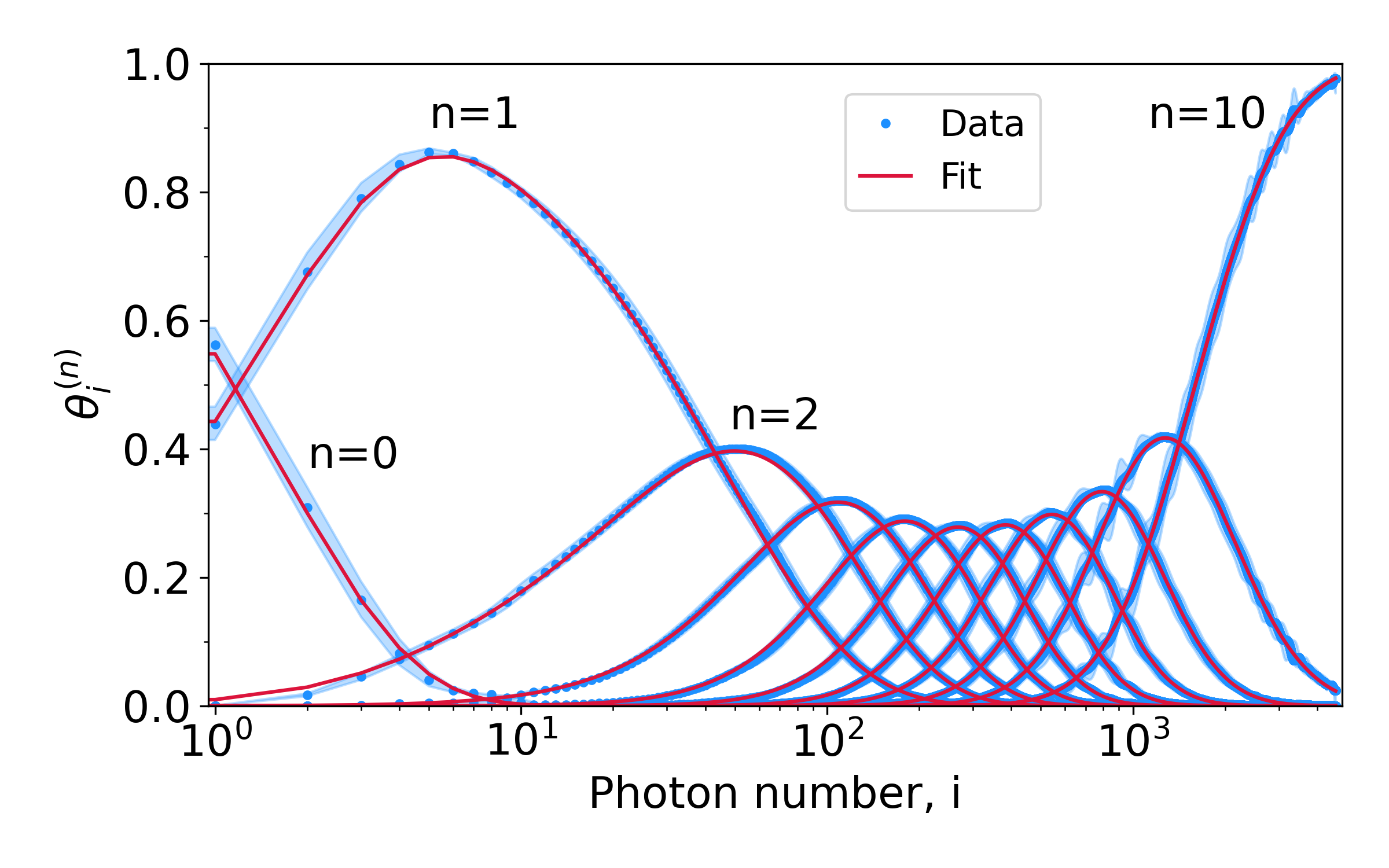
scaled by a factor $\epsilon$ , ensures that the resulting distributions are smooth Feito et al. 2009. For more details on the reconstruction process and importance of the correct choice of the smoothing parameter $\epsilon$ can be found in Ref. Schapeler et al. 2020. The reconstructed POVM elements for all eleven outcomes are shown in figure 2. The errors are calculated based on assuming 5% uncertainty in the amplitudes of the coherent states, which stems from the uncertainty in the calibration procedure.

Using the analysis from Ref. Schapeler et al. 2020 we can use the reconstructed POVMs to directly find figures of merit of the device. From this we find an overall device efficiency $\eta=0.44\pm 0.03$ , dark-count probability $p_{\mathrm{dark}}=(0.0+4.1)\times 10^{-7}$ and cross-talk probability $p_{\mathrm{xtalk}}=(4.6\pm 2.8)\times 10^{-6}$ .

The computational effort for the reconstruction depends on the size of the POVM matrix $\mathbf{\Pi}$ , i.e. the total number of outcomes $N$ and the Hilbert space dimension $M$ . Our current tomographic reconstruction method was able to reconstruct the POVM elements of the ten time-bin detector, however, due to limited computational power (3.6 GHz CPU with six cores and 16 GB RAM) this seems to be the limit of this implementation. Analysis of our code indicates that it is the smoothing function which consumes the most computation time and memory, and optimizing this routine would be the starting point for improving scalability.

Figure 3: Extrapolated POVMs using equations 2 and 6, shown up to

N=50

outcomes, corresponding to a Hilbert space dimension of

10^{6}

III.3 Extrapolation

From the experimental results, it is clear that our computational power limits us to reconstructing up to eleven outcomes reliably. However, to reconstruct higher-order POVMs, a different approach is required. The crux of this approach is to use parameters calculated in the low outcome regime and extrapolate this to higher order. This deviates a little in spirit from detector tomography, since it requires some modelling of the device. However, this technique can be used to test different models of the device, since it provides a bridge between the top-down (model-free) and bottom-up (first-principles) approaches to characterizing a detector.

The first assumption about our device is that each bin has a binary result: either “occupied” or “not occupied.” Outcomes of the detector correspond to the total number of occupied time-bins. As mentioned above, this can be considered as the result of a series of independent Bernoulli trials, where, in general, each trial can have a different success probability. The general form of the probability of $n$ out of $N_{\mathrm{bin}}$ time-bins being occupied, given an input Fock state $|i\rangle$ , is given by equation 2.

Using this formalism, an alternative approach to reconstructing the operation of the detector is to find the probabilities $p_{j}(i)$ for each bin to be occupied, given the input Fock states $|i\rangle$ for $i\in[0,M]$ , where $M$ is the Hilbert space dimension of the experimentally measured coherent input states. Note, however, this assumes that each bin is independent - this approach cannot account for conditional probabilities based on other bins firing, thus it cannot resolve effects like cross-talk.

In fact, for the loop detector considered in this paper, the probabilities $p_{j}(i)$ can be estimated by modelling the detector. From Ref. Tiedau et al. 2019 and neglecting dark counts (of the order $10^{-8}$ per time-bin), these probabilities are

p_{j}\left(i\right)=\Bigg\{\begin{array}[]{ll}1-\left(1-R\eta_{\mathrm{det}}\right)^{i}&j=1\\ 1-\left[1-\frac{\left(1-R\right)^{2}\eta_{\mathrm{det}}}{R}\left(R\eta_{\mathrm{loop}}\right)^{j-1}\right]^{i}&j\geq 2\end{array}\penalty\ ,

(6)

which have been adjusted to include the detection efficiency $\eta_{\mathrm{det}}$ . For the specific number of time-bins $N_{\mathrm{bin}}$ of the multiplexed detector, equation 2 depends on three parameters: the detection efficiency $\eta_{\mathrm{det}}$ , the out-coupling $R$ and the loop-efficiency $\eta_{\mathrm{loop}}$ . The optimal set of parameters can be found by fitting the Poisson binomial approximation, for all outcomes $n\in[0,10]$ simultaneously, to the experimental data. The fit is based on a minimization of the Frobenius norm between the experimental, and fit matrix and is shown in figure 2 together with the experimentally reconstructed POVMs. The fit revealed the parameters $\eta_{\mathrm{det}}=0.4912\pm\left(9\times 10^{-4}\right)$ , $R=0.89613\pm\left(8\times 10^{-5}\right)$ and $\eta_{\mathrm{loop}}=0.9064\pm\left(2\times 10^{-4}\right)$ .

Using these parameters and combining equations 2 and 6, we can then extrapolate the POVMs out to higher order. In figure 3 we show POVMs up to 50 outcomes, corresponding to a Hilbert space dimension of $10^{6}$ .

III.4 Verification using extrapolated POVMs

To show that the reconstructed POVMs of this device from the low photon-number and low outcome regime can be used to predict the behavior of the device for higher photon-numbers and outcomes, we use the model from equation 2 to extrapolate up to $N=120$ outcomes, which will be expressed in the matrix $\mathbf{\Pi^{\mathrm{ext}}}$ . We verify this by finding the mean photon number of a bright state.

In this experiment we subject the detector to one coherent input state generated from the same laser as in section III with a repetition rate of 50 kHz. The higher repetition rate enables a measurement of the mean photon number per pulse with a power meter. The train of pulses is again detected by the SNSPD (figure 1) and the output pulses are measured by a time-tagger in a histogram. We allow a total of $N_{\mathrm{bin}}=119$ time-bins, by choosing the histogram to consist of $1.87\times 10^{5}$ bins with a bin width of 100 ps. The measurement time is 300 s. By integrating over the raw bins we are able to find the probabilities of a specific bin $j\in[1,119]$ firing, which will be transformed into the probabilities $p^{\prime}_{n}$ of $n\in[0,119]$ time-bins being occupied, using equation 2. These probabilities then constitute the outcome matrix $\mathbf{P}$ .

Subsequently, we found the mean photon number of the bright state, by finding the coherent state which best fit the measurement data $\mathbf{P}$ and extrapolated POVMs $\mathbf{\Pi^{\mathrm{ext}}}$ by minimizing the expression

\left|\left|\mathbf{P}-\mathbf{F^{\mathrm{fit}}}\mathbf{\Pi^{\mathrm{ext}}}\right|\right|_{2}\penalty\ .

(7)

The resulting mean photon number of $\bar{n}^{\mathrm{fit}}=71000\pm 3000$ per pulse agrees with a separate measurement with a power meter of $(440\pm 22)$ pW, which results in a mean photon number of $\bar{n}^{\mathrm{pm}}=69000\pm 4000$ per pulse.

IV Conclusion

Characterizing the response of single-photon detectors is an important task in quantum optics. Configuring these detectors to be sensitive to bright states will become increasingly important as ever brighter photonic states become available Harder et al. 2016. Furthermore, having a self-consistent characterization of these detectors is important wherever they are utilized. We show that a tomographic reconstruction is possible even if the dynamic range of such a detector is extremely large. This is enabled by configuring a single-photon detector, in this case an SNSPD, to respond logarithmically to the number of photons. Nevertheless, the resulting photon number can be determined with very high accuracy. While we have demonstrated this method for a time-multiplexed system, we expect a similar approach to be applicable to spatially multiplexed arrays of superconducting detectors Miki et al. 2014; Allman et al. 2015; Shaw et al. 2015; Chen et al. 2019; Wollman et al. 2019.

Acknowledgements

We are grateful to Felix Dreher for assisting with data acquisition. This project is supported by the German Federal Ministry of Education and Research (BMBF) under the funding program Photonics Research Germany, grant number 13N14911.

References

Gol’Tsman et al. (2001) G. Gol’Tsman, O. Okunev, G. Chulkova, A. Lipatov, A. Semenov, K. Smirnov, B. Voronov, A. Dzardanov, C. Williams, and R. Sobolewski, Picosecond superconducting single-photon optical detector, Applied Physics Letters 79, 705 (2001).
Natarajan et al. (2012) C. M. Natarajan, M. G. Tanner, and R. H. Hadfield, Superconducting nanowire single-photon detectors: physics and applications, Superconductor Science and Technology 25, 063001 (2012).
Marsili et al. (2013) F. Marsili, V. B. Verma, J. A. Stern, S. Harrington, A. E. Lita, T. Gerrits, I. Vayshenker, B. Baek, M. D. Shaw, R. P. Mirin, and S. W. Nam, Detecting single infrared photons with 93% system efficiency, Nature Photonics 7, 210 (2013).
Shibata et al. (2015) H. Shibata, K. Shimizu, H. Takesue, and Y. Tokura, Ultimate low system dark-count rate for superconducting nanowire single-photon detector, Optics Letters 40, 3428 (2015).
Esmaeil Zadeh et al. (2017) I. Esmaeil Zadeh, J. W. N. Los, R. B. M. Gourgues, V. Steinmetz, G. Bulgarini, S. M. Dobrovolskiy, V. Zwiller, and S. N. Dorenbos, Single-photon detectors combining high efficiency, high detection rates, and ultra-high timing resolution, APL Photonics 2, 111301 (2017).
Korzh et al. (2020) B. Korzh, Q.-Y. Zhao, J. P. Allmaras, S. Frasca, T. M. Autry, E. A. Bersin, A. D. Beyer, R. M. Briggs, B. Bumble, M. Colangelo, G. M. Crouch, A. E. Dane, T. Gerrits, A. E. Lita, F. Marsili, G. Moody, C. Peña, E. Ramirez, J. D. Rezac, N. Sincliar, M. J. Stevens, A. E. Velasco, V. B. Verma, E. E. Wollman, S. Xie, D. Zhu, P. D. Hale, M. Spiropulu, K. L. Silverman, R. P. Mirin, S. W. Nam, A. G. Kozorezov, M. D. Shaw, and K. K. Berggren, Demonstration of sub-3 ps temporal resolution with a superconducting nanowire single-photon detector, Nature Photonics 14, 250 (2020).
Cahall et al. (2017) C. Cahall, K. L. Nicolich, N. T. Islam, G. P. Lafyatis, A. J. Miller, D. J. Gauthier, and J. Kim, Multi-photon detection using a conventional superconducting nanowire single-photon detector, Optica 4, 1534 (2017).
Zhu et al. (2018) D. Zhu, Q.-Y. Zhao, H. Choi, T.-J. Lu, A. E. Dane, D. Englund, and K. K. Berggren, A scalable multi-photon coincidence detector based on superconducting nanowires, Nature Nanotechnol. 13, 596 (2018).
Zhu et al. (2020) D. Zhu, M. Colangelo, C. Chen, B. A. Korzh, F. N. Wong, M. D. Shaw, and K. K. Berggren, Resolving Photon Numbers Using a Superconducting Nanowire with Impedance-Matching Taper, Nano Letters 20, 3858 (2020).
Zou et al. (2020) K. Zou, Y. Meng, Z. Wang, and X. Hu, Superconducting nanowire multi-photon detectors enabled by current reservoirs, Photonics Research 8, 601 (2020).
Dauler et al. (2007) E. A. Dauler, B. S. Robinson, A. J. Kerman, J. K. W. Yang, K. M. Rosfjord, V. Anant, B. Voronov, G. Gol’tsman, and K. K. Berggren, Multi-Element Superconducting Nanowire Single-Photon Detector, IEEE Trans. Appl. Supercond. 17, 279 (2007).
Divochiy et al. (2008) A. Divochiy, F. Marsili, D. Bitauld, A. Gaggero, R. Leoni, F. Mattioli, A. Korneev, V. Seleznev, N. Kaurova, O. Minaeva, G. Gol’tsman, K. G. Lagoudakis, M. Benkhaoul, F. Lévy, and A. Fiore, Superconducting nanowire photon-number-resolving detector at telecommunication wavelengths, Nature Photonics 2, 302 (2008).
Marsili et al. (2009) F. Marsili, D. Bitauld, A. Gaggero, S. Jahanmirinejad, R. Leoni, F. Mattioli, and A. Fiore, Physics and application of photon number resolving detectors based on superconducting parallel nanowires, New Journal of Physics 11, 045022 (2009).
Jahanmirinejad et al. (2012) S. Jahanmirinejad, G. Frucci, F. Mattioli, D. Sahin, A. Gaggero, R. Leoni, and A. Fiore, Photon-number resolving detector based on a series array of superconducting nanowires, Applied Physics Letters 101, 072602 (2012).
Zhao et al. (2013) Q. Zhao, A. McCaughan, F. Bellei, F. Najafi, D. De Fazio, A. Dane, Y. Ivry, and K. K. Berggren, Superconducting-nanowire single-photon-detector linear array, Applied Physics Letters 103, 142602 (2013).
Rosenberg et al. (2013) D. Rosenberg, A. J. Kerman, R. J. Molnar, and E. A. Dauler, High-speed and high-efficiency superconducting nanowire single photon detector array, Optics Express 21, 1440 (2013).
Verma et al. (2014) V. B. Verma, R. Horansky, F. Marsili, J. A. Stern, M. D. Shaw, A. E. Lita, R. P. Mirin, and S. W. Nam, A four-pixel single-photon pulse-position array fabricated from WSi superconducting nanowire single-photon detectors, Applied Physics Letters 104, 051115 (2014).
Miki et al. (2014) S. Miki, T. Yamashita, Z. Wang, and H. Terai, A 64-pixel NbTiN superconducting nanowire single-photon detector array for spatially resolved photon detection, Optics Express 22, 7811 (2014).
Allman et al. (2015) M. S. Allman, V. B. Verma, M. Stevens, T. Gerrits, R. D. Horansky, A. E. Lita, F. Marsili, A. Beyer, M. D. Shaw, D. Kumor, R. Mirin, and S. W. Nam, A near-infrared 64-pixel superconducting nanowire single photon detector array with integrated multiplexed readout, Applied Physics Letters 106, 192601 (2015).
Shaw et al. (2015) M. D. Shaw, F. Marsili, A. D. Beyer, J. A. Stern, G. V. Resta, P. Ravindran, S. Chang, J. Bardin, D. S. Russell, J. W. Gin, F. D. Patawaran, V. B. Verma, R. P. Mirin, S. W. Nam, and W. H. Farr, Arrays of WSi Superconducting Nanowire Single Photon Detectors for Deep-Space Optical Communications, in 2015 Conference on Lasers and Electro-Optics (CLEO). IEEE (2015).
Najafi et al. (2015) F. Najafi, J. Mower, N. C. Harris, F. Bellei, A. Dane, C. Lee, X. Hu, P. Kharel, F. Marsili, S. Assefa, K. K. Berggren, and D. Englund, On-chip detection of non-classical light by scalable integration of single-photon detectors, Nature Communications 6, 5873 (2015).
Chen et al. (2019) Q. Chen, B. Zhang, L. Zhang, R. Ge, R. Xu, Y. Wu, X. Tu, X. Jia, D. Pan, L. Kang, et al., Sixteen-pixel nbn nanowire single photon detector coupled with 300- $\mu$ m fiber, IEEE Photonics Journal 12, 1 (2019).
Tao et al. (2019) X. Tao, S. Chen, Y. Chen, L. Wang, X. Li, X. Tu, X. Jia, Q. Zhao, L. Zhang, L. Kang, et al., A high speed and high efficiency superconducting photon number resolving detector, Superconductor Science and Technology 32, 064002 (2019).
Wollman et al. (2019) E. E. Wollman, V. B. Verma, A. E. Lita, W. H. Farr, M. D. Shaw, R. P. Mirin, and S. W. Nam, Kilopixel array of superconducting nanowire single-photon detectors, Optics Express 27, 35279 (2019).
Natarajan et al. (2013) C. M. Natarajan, L. Zhang, H. Coldenstrodt-Ronge, G. Donati, S. N. Dorenbos, V. Zwiller, I. A. Walmsley, and R. H. Hadfield, Quantum detector tomography of a time-multiplexed superconducting nanowire single-photon detector at telecom wavelengths, Optics Express 21, 893 (2013).
Tiedau et al. (2019) J. Tiedau, E. Meyer-Scott, T. Nitsche, S. Barkhofen, T. J. Bartley, and C. Silberhorn, A high dynamic range optical detector for measuring single photons and bright light, Optics Express 27, 1 (2019).
Jönsson et al. (2020) M. Jönsson, M. Swillo, S. Gyger, V. Zwiller, and G. Björk, Temporal array with superconducting nanowire single-photon detectors for photon-number resolution, Physical Review A 102, 052616 (2020).
Lundeen et al. (2009) J. Lundeen, A. Feito, H. Coldenstrodt-Ronge, K. Pregnell, C. Silberhorn, T. Ralph, J. Eisert, M. Plenio, and I. Walmsley, Tomography of quantum detectors, Nature Physics 5, 27 (2009).
Akhlaghi et al. (2011) M. K. Akhlaghi, A. H. Majedi, and J. S. Lundeen, Nonlinearity in single photon detection: modeling and quantum tomography, Optics Express 19, 21305 (2011).
Renema et al. (2012) J. Renema, G. Frucci, Z. Zhou, F. Mattioli, A. Gaggero, R. Leoni, M. De Dood, A. Fiore, and M. Van Exter, Modified detector tomography technique applied to a superconducting multiphoton nanodetector, Optics Express 20, 2806 (2012).
Endo et al. (2021) M. Endo, T. Sonoyama, M. Matsuyama, F. Okamoto, S. Miki, M. Yabuno, F. China, H. Terai, and A. Furusawa, Quantum detector tomography of superconducting nanostrip photon-number-resolving detector (2021), arXiv:2102.09712 [quant-ph] .
Schapeler et al. (2020) T. Schapeler, J. P. Höpker, and T. J. Bartley, Quantum detector tomography of a 2 $\times$ 2 multi-pixel array of superconducting nanowire single photon detectors, Optics Express 28, 33035 (2020).
Wang (1993) Y. H. Wang, On the number of successes in independent trials, Statistica Sinica 3, 295 (1993).
Fernández and Williams (2010) M. Fernández and S. Williams, Closed-form expression for the poisson-binomial probability density function, IEEE Transactions on Aerospace and Electronic Systems 46, 803 (2010).
Golub and Van Loan (2013) G. Golub and C. Van Loan, Matrix Computations, Johns Hopkins Studies in the Mathematical Sciences (Johns Hopkins University Press, 2013).
Feito et al. (2009) A. Feito, J. Lundeen, H. Coldenstrodt-Ronge, J. Eisert, M. B. Plenio, and I. A. Walmsley, Measuring measurement: theory and practice, New Journal of Physics 11, 093038 (2009).
Harder et al. (2016) G. Harder, T. J. Bartley, A. E. Lita, S. W. Nam, T. Gerrits, and C. Silberhorn, Single-mode parametric-down-conversion states with 50 photons as a source for mesoscopic quantum optics, Physical Review Letters 116, 143601 (2016).