跳到论文正文
W Papers独立论文阅读器 arXiv:2102.11568 论文正文 计算阅读时间 · 0%
引用这篇论文根据当前论文元数据生成,正式投稿前建议核对。


License: arXiv.org perpetual non-exclusive license
arXiv:2102.11568v2 [math.PR] 12 Mar 2021

Sharp moment estimates for martingales
with uniformly bounded square functions Thanks: Supported by the Russian Science Foundation Grant 19-71-10023.

Dmitriy Stolyarov    Vasily Vasyunin    Pavel Zatitskiy    Ilya Zlotnikov
Abstract

We provide sharp bounds for the exponential moments and pp-moments, 1⩽p⩽21\leqslant p\leqslant 2, of the terminate distribution of a martingale whose square function is uniformly bounded by one. We introduce a Bellman function for the corresponding extremal problem and reduce it to the already known Bellman function on BMO⁡([0,1])\mathrm{BMO}([0,1]). In the case of tail estimates, a similar reduction does not work exactly, so we come up with a fine supersolution that leads to sharp tail estimates.

1 Introduction

1.1 Chang–Wilson–Wolff inequality

Let (X,Σ,P)(X,\Sigma,P) be an atomless complete probability space equipped with a discrete time filtration ℱ={ℱn}n⩾0\mathcal{F}=\{\mathcal{F}_{n}\}_{n\geqslant 0}. Let ℱ0={∅,X}\mathcal{F}_{0}=\{\varnothing,X\} and let ℱ\mathcal{F} generate Σ\Sigma. Assume for simplicity that each σ\sigma-algebra ℱn\mathcal{F}_{n} is finite, i. e., consists of a finite number of sets. Consider a real-valued martingale φ={φn}n\varphi=\{\varphi_{n}\}_{n} adapted to ℱ\mathcal{F} and define its square function S​φS\varphi by the formula

S​φ=(∑n=0∞(φn+1−φn)2)12.S\varphi=\Big(\sum\limits_{n=0}^{\infty}(\varphi_{n+1}-\varphi_{n})^{2}\Big)^{\frac{1}{2}}. (1.1)

In what follows we will always talk about real martingales adapted to filtrations as above unless otherwise specified. We call a martingale φ\varphi simple if φn+1=φn\varphi_{n+1}=\varphi_{n} for nn sufficiently large. In this paper, we make an attempt to describe the distribution of φ∞\varphi_{\infty} (which is the limit value of the martingale, φ∞=limn→∞φn\varphi_{\infty}=\lim_{n\to\infty}\varphi_{n}) under the assumption that S​φS\varphi is uniformly bounded. From general theory (see (1.5) below), φ\varphi is a BMO\mathrm{BMO}-martingale provided S​φ∈L∞S\varphi\in L_{\infty}. Thus, by the John–Nirenberg inequality, φ∞\varphi_{\infty} is a subexponential random variable. Namely, there exist positive constants c1c_{1} and c2c_{2} such that

P⁡(φ∞−φ0⩾t)⩽c2​e−c1​t‖S​φ‖L∞,t>0,P(\varphi_{\infty}-\varphi_{0}\geqslant t)\leqslant c_{2}e^{-\frac{c_{1}t}{\ \|S\varphi\|_{L_{\infty}}}},\qquad t>0, (1.2)

for any martingale φ\varphi. We focus on sharp estimates of this kind. In particular, we aim to compute the best possible values of c1c_{1} and c2c_{2} (see Corollary 1.14 below). According to the knowledge of the authors, such sharp estimates are not known.

In the case where ℱ\mathcal{F} is a dyadic filtration (by that we mean that any atom in ℱn\mathcal{F}_{n} is split into two atoms of equal mass in ℱn+1\mathcal{F}_{n+1}), a much better estimate exists. The famous Chang–Wilson–Wolff inequality (see Theorem 3.1 in [2] for the original formulation and [19] for further development) says that the distribution of φ\varphi is subgaussian:

P⁡(φ∞−φ0⩾t)⩽e−t2 2​‖S​φ‖L∞2,t>0.P(\varphi_{\infty}-\varphi_{0}\geqslant t)\leqslant e^{-\frac{t^{2}}{\ 2\|S\varphi\|^{2}_{L_{\infty}}}},\qquad t>0. (1.3)

In a recent paper [8], Ivanisvili and Treil generalized this result to the case where the filtration ℱ\mathcal{F} has bounded distortion α\alpha, which means that each atom in ℱn\mathcal{F}_{n} has at least α\alpha mass of its parental atom. In this case,

P⁡(φ∞−φ0⩾t)⩽e−α​t2‖S​φ‖L∞2,t>0.P(\varphi_{\infty}-\varphi_{0}\geqslant t)\leqslant e^{-\frac{\alpha t^{2}}{\ \|S\varphi\|^{2}_{L_{\infty}}}},\qquad t>0. (1.4)

This result hints us that the distribution of φ∞\varphi_{\infty} may no longer be subgaussian if we do not make assumptions about regularity of the filtration. As we will see later, this is indeed the case (for example, the inequality (1.2) is sharp for certain choice of c1c_{1} and c2c_{2}, see Corollary 1.14 below).

Since we focus on sharp estimates, it is natural to consider not only tail estimates, but also inequalities for the exponential moments and pp-moments. In particular, one may wonder what are the largest possible values of the quantities 𝔼⁡eλ​φ∞\E e^{\lambda\varphi_{\infty}}, or 𝔼⁡|φ∞|p\E|\varphi_{\infty}|^{p} under the assumption ‖S​φ‖L∞⩽1\|S\varphi\|_{L_{\infty}}\leqslant 1. We will partially answer this question, see Corollaries 1.11 and 1.12 below. One may go further, pick an arbitrary function ff, and ask about the largest possible value of 𝔼⁡f⁡(φ∞)\E f(\varphi_{\infty}) under the same assumption. We will study this problem for the cases when f′′′f^{\prime\prime\prime} either does not change sign or changes sign from ++ to −- once.

Some of the results of the present paper were announced in the short report [21]. We also provided some proofs there. The present paper contains the remaining proofs. In a sense, [21] contains the reasoning that do not depend on the geometry of specific Bellman functions. They are much shorter than the treatment of Bellman functions we present here.

For the reader who is not interested in the Bellman function technique, Corollaries 1.11, 1.12, and 1.14 may be considered as the main results of the paper. Lemma 1.8 and Theorems 1.10 and 1.13 are more important from the Bellman function point of view.

1.2 Estimates for BMO\mathrm{BMO} functions

The space BMO\mathrm{BMO} is pivotal for our considerations. There are several equivalent norms in this space. Since we are dealing with sharp estimates, the choice of a specific norm is crucial. The space BMOm\mathrm{BMO}^{\mathrm{m}} called the space of martingales of bounded mean oscillation is defined as follows (see, e. g., Chapter II in [9])

‖φ‖BMOm2=sup{‖𝔼⁡((φ∞−φτ)2∣ℱτ)‖L∞|τ​ is a stopping time}.\|\varphi\|_{\mathrm{BMO}^{\mathrm{m}}}^{2}=\sup\Big\{\big\|\E\big((\varphi_{\infty}-\varphi_{\tau})^{2}\mid\mathcal{F}_{\tau}\big)\big\|_{L_{\infty}}\,\Big|\;\tau\text{ is a stopping time}\Big\}.

A simple orthogonality argument

𝔼⁡((φ∞−φτ)2∣ℱτ)=𝔼⁡((∑n⩾τ(φn+1−φn))2|ℱτ)=𝔼⁡(∑n⩾τ(φn+1−φn)2|ℱτ)⩽𝔼⁡((S​φ)2∣ℱτ),\E\big((\varphi_{\infty}-\varphi_{\tau})^{2}\mid\mathcal{F}_{\tau}\big)=\E\Big(\Big(\sum\limits_{n\geqslant\tau}(\varphi_{n+1}-\varphi_{n})\Big)^{2}\,\Big|\;\mathcal{F}_{\tau}\Big)=\\ \E\Big(\sum\limits_{n\geqslant\tau}(\varphi_{n+1}-\varphi_{n})^{2}\,\Big|\;\mathcal{F}_{\tau}\Big)\leqslant\E\big((S\varphi)^{2}\mid\mathcal{F}_{\tau}\big), (1.5)

leads to the inequality ‖φ‖BMOm⩽‖S​φ‖L∞\|\varphi\|_{\mathrm{BMO}^{\mathrm{m}}}\leqslant\|S\varphi\|_{L_{\infty}}.

The space BMOm\mathrm{BMO}^{\mathrm{m}} has its real analysis counterpart (see, e. g., Chapter IV in [20] for more information). The BMO\mathrm{BMO} space on the unit interval is defined with the help of the seminorm

‖ψ‖BMO⁡([0,1])2=sup{1|J|​∫J(ψ⁡(x)−1|J|​∫Jψ)2​𝑑x|J​ is a subinterval of ​[0,1]}.\|\psi\|_{\mathrm{BMO}([0,1])}^{2}=\sup\Big\{\frac{1}{|J|}\int\limits_{J}\Big(\psi(x)-\frac{1}{|J|}\int\limits_{J}\psi\Big)^{2}dx\;\Big|\,J\text{ is a subinterval of }[0,1]\Big\}. (1.6)

We note that this definition is not the most common in real analysis. A version based on the L1L_{1} norm instead of L2L_{2} is more widespread (the two BMO\mathrm{BMO} seminorms are equivalent). The L2L_{2} based version is closely related to the martingale BMOm\mathrm{BMO}^{\mathrm{m}} space. We denote the non-increasing rearrangement (the inverse function to the distribution function of ξ\xi) of a random variable ξ\xi by ξ∗\xi^{*}:

ξ∗​(t)=inf{α∣P⁡(ξ>α)⩽t},t∈[0,1).\xi^{*}(t)=\inf\{\alpha\mid P(\xi>\alpha)\leqslant t\},\qquad t\in[0,1).
Theorem 1.1.

The inequality ‖φ∞∗‖BMO⁡([0,1])⩽‖S​φ‖L∞\|\varphi_{\infty}^{*}\|_{\mathrm{BMO}([0,1])}\leqslant\|S\varphi\|_{L_{\infty}} holds for any martingale φ\varphi and is sharp.

Here and in what follows the notation φ∞∗\varphi_{\infty}^{*} means the monotonic rearrangement of φ∞\varphi_{\infty}. This theorem was proved in [21]. Though Theorem 1.1 says there is a certain relationship between martingales φ\varphi whose square function is bounded and functions ψ\psi on the unit interval that belong to the BMO\mathrm{BMO} space, we warn the reader against identification of these classes of objects, which have different nature and origin.

Remark 1.2.

The estimate ‖φ∞∗‖BMO⁡([0,1])⩽‖φ‖BMOm\|\varphi_{\infty}^{*}\|_{\mathrm{BMO}([0,1])}\leqslant\|\varphi\|_{\mathrm{BMO}^{\mathrm{m}}} is not true in general for discrete time filtrations. To see that, consider the case where ℱ\mathcal{F} is dyadic. The inequality

‖φ∞∗‖BMO⁡([0,1])⩽32​2​‖φ‖BMOm,ℱ​ is dyadic,\|\varphi_{\infty}^{*}\|_{\mathrm{BMO}([0,1])}\leqslant\frac{3}{2\sqrt{2}}\|\varphi\|_{\mathrm{BMO}^{\mathrm{m}}},\quad\mathcal{F}\hbox{ is dyadic},

is sharp (and true), see Corollary 11 in [22]. What is more, for any C>0C>0 there exist a discrete filtration ℱ\mathcal{F} and a martingale φ\varphi adapted to it such that the inequality

‖φ∞∗‖BMO⁡([0,1])⩽C​‖φ‖BMOm\|\varphi_{\infty}^{*}\|_{\mathrm{BMO}([0,1])}\leqslant C\|\varphi\|_{\mathrm{BMO}^{\mathrm{m}}}

fails.

Theorem 1.1 leads to many nice inequalities. In particular, it says that

sup{𝔼f(φ∞)|φ0=x,∥Sφ∥L∞⩽1}⩽sup{∫01f(ψ)|∫01ψ=x,∥ψ∥BMO⁡([0,1])⩽1}{\sup\Big\{\E f(\varphi_{\infty})\,\Big|\;\varphi_{0}=x,\;\|S\varphi\|_{L_{\infty}}\leqslant 1\Big\}\leqslant\sup\Big\{\int\limits_{0}^{1}f(\psi)\,\Big|\,\int\limits_{0}^{1}\psi=x,\;\|\psi\|_{\mathrm{BMO}([0,1])}\leqslant 1\Big\}} (1.7)

for any non-negative function f:ℝ→ℝf\colon\mathbb{R}\to\mathbb{R}. It is reasonable to fix the expectation of our martingale since φ0\varphi_{0} does not affect the square function, but has strong influence on the quantity 𝔼⁡f⁡(φ∞)\E f(\varphi_{\infty}). There are two surprising facts about formula (1.7). The first one is that the inequality turns into equality quite often (in particular, for the important cases f⁡(t)=eλ​tf(t)=e^{\lambda t} and f⁡(t)=|t|p,1⩽p⩽2f(t)=|t|^{p},1\leqslant p\leqslant 2). The second fact is that the supremum on the right hand side may be computed exactly for arbitrary ff, which satisfies some mild regularity assumptions. We briefly describe these results.

We fix the second moment as well and write the definition of the Bellman function bε:ωε→ℝb_{\varepsilon}\colon\omega_{\varepsilon}\to\mathbb{R},

bε​(x,y)\displaystyle b_{\varepsilon}(x,y) =sup{∫01f(ψ)|∫01ψ=x,∫01ψ2=y,∥ψ∥BMO⁡([0,1])⩽ε},\displaystyle=\sup\bigg\{\int\limits_{0}^{1}f(\psi)\,\bigg|\;\int_{0}^{1}\!\psi=x,\;\int_{0}^{1}\!\psi^{2}=y,\ \|\psi\|_{\mathrm{BMO}([0,1])}\leqslant\varepsilon\bigg\}, (1.8)
ωε\displaystyle\omega_{\varepsilon} ={(x,y)∈ℝ2∣x2⩽y⩽x2+ε2}.\displaystyle=\{(x,y)\in\mathbb{R}^{2}\mid x^{2}\leqslant y\leqslant x^{2}+\varepsilon^{2}\}.

This Bellman function satisfies the boundary condition bε​(x,x2)=f⁡(x)b_{\varepsilon}(x,x^{2})=f(x). It appears that one may compute the function bεb_{\varepsilon} for arbitrary ff. The answer (algorithm) is quite complicated. We refer the reader to the paper [7] for treatment of the general case. The paper [6] considers less general case (the authors make additional assumptions on the structure of ff), however, provides a much shorter presentation. The short report [5] outlines the results. In fact, the particular cases that are important for applications were computed in earlier papers [17], [18], [24], and [26].

The main reason why bεb_{\varepsilon} is a tractable object is that it can be described geometrically, namely, in terms of locally concave functions. By a locally concave function on a domain we mean a function whose restriction to any segment lying in the domain entirely, is concave.

Theorem 1.3 (Main theorem and Corollary 5.4 in [23]).

Let ff be bounded from below. The function bεb_{\varepsilon} can be described as the pointwise minimal function among all locally concave functions G:ωε→ℝG\colon\omega_{\varepsilon}\to\mathbb{R} that satisfy the boundary condition G⁡(x,x2)=f⁡(x)G(x,x^{2})=f(x).

The fact behind Theorem 1.3 is that the minimal locally concave function has a good probabilistic representation, see Theorem 2.21 in [23]. We cite a definition introduced in [23] (in fact, [23] deals with a more general situation; in the case of BMO\mathrm{BMO} and the parabolic strip ωε\omega_{\varepsilon} the continuous time version of the definition below had appeared in the literature before [23], see, e. g., [9] and [16]; as the present paper shows, the discrete time definition is more convenient in some contexts).

Definition 1.4.

An ℝ2\mathbb{R}^{2}-valued martingale M={Mn}nM=\{M_{n}\}_{n} adapted to {ℱn}n\{\mathcal{F}_{n}\}_{n} is called an ωε\omega_{\varepsilon}-martingale if it satisfies the conditions listed below.

  1. 1.

    ℱ0={∅,X}\mathcal{F}_{0}=\{\varnothing,X\}.

  2. 2.

    There exists a random variable M∞M_{\infty} with values in {(t,t2)∣t∈ℝ}\{(t,t^{2})\mid t\in\mathbb{R}\} such that

    𝔼⁡|M∞|<∞andMn=𝔼⁡(M∞∣ℱn).\E|M_{\infty}|<\infty\quad\hbox{and}\quad M_{n}=\E(M_{\infty}\mid\mathcal{F}_{n}).
  3. 3.

    For every n∈ℤ+n\in\mathbb{Z}_{+} and every atom σ\sigma in ℱn\mathcal{F}_{n}

    conv⁡{Mn+1​(z)}z∈σ⊂ωε.\conv\{M_{n+1}(z)\}_{z\in\sigma}\subset\omega_{\varepsilon}.

The third requirement should be understood properly: we define Mn=𝔼⁡(M∞∣ℱn)M_{n}=\E(M_{\infty}\mid\mathcal{F}_{n}) everywhere and thus, consider the convex hull of a finite number of points. By conv⁡A\conv A we denote the convex hull of a set AA.

The following lemma plays a crucial role in the proof of Theorem 1.1.

Lemma 1.5 (Theorem 3.4 in [23]).

Let MM be an ωε\omega_{\varepsilon} martingale. The random variable M∞1M_{\infty}^{1} (the first coordinate of the ℝ2\mathbb{R}^{2}-valued random variable M∞M_{\infty}) satisfies the inequality

‖(M∞1)∗‖BMO⁡([0,1])⩽ε.{\|(M_{\infty}^{1})^{*}\|_{\mathrm{BMO}([0,1])}\leqslant\varepsilon.} (1.9)

1.3 Our results

The function f:ℝ→ℝf\colon\mathbb{R}\to\mathbb{R} will be subject to some requirements. We will always assume ff is measurable and non-negative. Of course, one may use a slightly weaker assumption that ff is uniformly bounded from below (or replacing ff with −f-f, that ff is bounded from above). Sometimes we will need a regularity assumption.

Definition 1.6.

We say that ff satisfies the standard requirements if it is a non-negative twice continuously differentiable function, its third distributional derivative is a signed measure, which changes sign only finite number of times, and

∫ℝe−|t|ε​|d​f′′​(t)|​<∞for someε>​1.{\int\limits_{\mathbb{R}}e^{-\frac{|t|}{\varepsilon}}|df^{\prime\prime}(t)|<\infty\qquad\hbox{for some}\quad\varepsilon>1.} (1.10)

These requirements for ff are slightly stronger than in [7] (the authors of that paper did not require the positivity of ff). Note that the choices f⁡(t)=|t|pf(t)=|t|^{p}, p∈[1,2)p\in[1,2), and f(t)=χ[0,∞)(t)f(t)=\chi_{{}_{[0,\infty)}}(t) do not satisfy the standard requirements (the first one is quite close, while the second function is very far from being C2C^{2}-smooth).

We introduce the main character:

𝑩(x,y,z)=sup{𝔼Hf(φ∞,(Sφ)2+z2)|𝔼φ∞=x,𝔼φ∞2=y},z⩾0,\boldsymbol{B}(x,y,z)=\sup\Big\{\E H_{f}(\varphi_{\infty},(S\varphi)^{2}+z^{2})\,\Big|\;\E\varphi_{\infty}=x,\ \E\varphi_{\infty}^{2}=y\Big\},\quad z\geqslant 0, (1.11)

where

Hf​(s,t)={−∞,t∉[0,1];f(s),t∈[0,1],H_{f}(s,t)=\begin{cases}-\infty,\quad&t\notin[0,1];\\ f(s),\quad&t\in[0,1],\end{cases}

and the supremum is taken over all simple martingales φ\varphi adapted to a discrete time filtration. We consider only simple martingales here to avoid technicalities. Note that it suffices to work with simple martingales to obtain sharp constants in the inequalities (1.15), (1.16), and (1.22) below.

This Bellman function will help us to find sharp constants in several inequalities. The reader familiar with the Burkholder method (see the original papers [1] and [10] or the books [12], [25]) may say that the yy-coordinate is redundant. However, we prefer to keep it, because it ‘‘tracks’’ the Hilbert space identities that link the square function to the martingale itself.

Remark 1.7.

For any x,yx,y fixed, the function z↦𝐁⁡(x,y,z)z\mapsto\boldsymbol{B}(x,y,z) is non-increasing. This follows from formula (1.11), more specifically, from an equivalent formula

𝑩(x,y,z)=sup{𝔼f(φ∞)|𝔼φ∞=x,𝔼φ∞2=y,Sφ⩽1−z2a. s.}.\boldsymbol{B}(x,y,z)=\sup\Big\{\E f(\varphi_{\infty})\,\Big|\;\E\varphi_{\infty}=x,\;\E\varphi_{\infty}^{2}=y,\;S\varphi\leqslant\sqrt{1-z^{2}}\ \text{a.\,s.}\,\Big\}. (1.12)

As we will prove a little bit later (see Lemma 2.1 below), the natural domain for 𝑩\boldsymbol{B} is

Ω={(x,y,z)∈ℝ3|x2⩽y⩽1−z2+x2,z∈[0,1]}.\Omega=\Big\{(x,y,z)\in\mathbb{R}^{3}\,\Big|\;x^{2}\leqslant y\leqslant 1-z^{2}+x^{2},\quad z\in[0,1]\Big\}. (1.13)

We start with the Bellman function counterpart of Theorem 1.1. Recall the function bεb_{\varepsilon} defined in (1.8).

Lemma 1.8.

Let ff be a non-negative function. The inequality 𝐁⁡(x,y,z)⩽b1−z2​(x,y)\boldsymbol{B}(x,y,z)\leqslant b_{\sqrt{1-z^{2}}}(x,y) is true for any triple (x,y,z)∈Ω(x,y,z)\in\Omega.

This lemma implies (1.7) (plug z=0z=0 and optimize with respect to yy). It has already appeared in [21]. We present its proof in Section 2 for completeness (in fact, the arguments are quite elementary here).

Corollary 1.9.

Let a measurable function h:ℝ→ℝ+h\colon\mathbb{R}\to\mathbb{R}_{+} satisfy

∑k∈ℤe−|k|​supx∈[k−2,k+2]h⁡(x)<∞.{\sum\limits_{k\in\mathbb{Z}}e^{-|k|}\sup\limits_{x\in[k-2,k+2]}h(x)<\infty.} (1.14)

Then the quantity 𝔼⁡h⁡(φ∞)\E h(\varphi_{\infty}) is finite for any martingale φ\varphi such that S​φ⩽1S\varphi\leqslant 1 almost surely. The bound is uniform with respect to φ\varphi as long as φ0\varphi_{0} is fixed.

This corollary will be proved in Section 2. It is sharp in certain sense. For example, one may construct a C3C^{3}-smooth function hh such that h′′′⩾0h^{\prime\prime\prime}\geqslant 0 and h⁡(x)=ex/xh(x)=e^{x}/x when xx is sufficiently large. Theorem 1.10 below then says 𝑩⁡(x,y,z)=b1−z2​(x,y)\boldsymbol{B}(x,y,z)=b_{\sqrt{1-z^{2}}}(x,y) if both these functions are constructed for f:=hf:=h. However, one may see that with this function hh the Bellman function b1b_{1} is infinite since the integral ∫01h⁡(ψ)\int_{0}^{1}h(\psi) diverges if one plugs ψ⁡(t)=−log⁡t\psi(t)=-\log t into (1.8) (the function log⁡t\log t has BMO\mathrm{BMO}-norm equal to one).

As we have said, the inequality in Lemma 1.8 often turns into equality.

Theorem 1.10.

Assume ff satisfies the standard requirements and either f′′f^{\prime\prime} is monotone or f′′f^{\prime\prime} increases up to some point and then decreases. Then, 𝐁⁡(x,y,z)=b1−z2​(x,y)\boldsymbol{B}(x,y,z)=b_{\sqrt{1-z^{2}}}(x,y) for all (x,y,z)∈Ω(x,y,z)\in\Omega.

Theorem 1.10 was also stated in [21], but was not proved. Its proof is presented in Subsection 3.3. Note that particular choices f⁡(t)=eλ​tf(t)=e^{\lambda t} and f⁡(t)=|t|pf(t)=|t|^{p}, 1⩽p⩽21\leqslant p\leqslant 2 (this function does not satisfy the standard requirements, however, we will be able to cope with this difficulty), fit the assumptions of Theorem 1.10. The corresponding functions bεb_{\varepsilon} were computed in [17] and [18] respectively. These results will lead us to the corollaries below.

Corollary 1.11.

The optimal constant cpc_{p} in the inequality

‖φ∞−φ0‖Lp⩽cp​‖S​φ‖L∞\|\varphi_{\infty}-\varphi_{0}\|_{L_{p}}\leqslant c_{p}\|S\varphi\|_{L_{\infty}} (1.15)

equals 11 when 1⩽p⩽21\leqslant p\leqslant 2.

Corollary 1.12.

The optimal constant C⁡(ε)C(\varepsilon) in the inequality

𝔼⁡eφ−φ0⩽C⁡(ε),S​φ⩽ε.\E e^{\varphi-\varphi_{0}}\leqslant C(\varepsilon),\quad S\varphi\leqslant\varepsilon. (1.16)

equals e−ε1−ε\frac{e^{-\varepsilon}}{1-\varepsilon} when ε<1\varepsilon<1.

Sometimes the inequality in Lemma 1.8 is strict on a subdomain of Ω\Omega. We present the following example corresponding to the choice f(t)=χ[0,∞)(t)f(t)=\chi_{{}_{[0,\infty)}}(t). Note that this function does not fulfill the standard requirements (however, this is not the reason for failure of the equality between the Bellman functions; we consider this example since it leads to sharp constants in the inequality (1.2)). In this case, the function bεb_{\varepsilon} was computed in [24]. The domain ωε\omega_{\varepsilon} is split into four parts (see Figure 1)

D1ε\displaystyle D_{1}^{\varepsilon} ={(x,y)∈ωε∣y⩾2εx,x⩾ε}∪{(x,y)∈ωε∣y⩽2εx};\displaystyle=\{(x,y)\in\omega_{\varepsilon}\mid y\geqslant 2\varepsilon x,\;x\geqslant\varepsilon\}\cup\{(x,y)\in\omega_{\varepsilon}\mid y\leqslant 2\varepsilon x\}; (1.17)
D2ε\displaystyle D_{2}^{\varepsilon} ={(x,y)∈ωε∣|x|⩽ε,y⩾2ε|x|};\displaystyle=\{(x,y)\in\omega_{\varepsilon}\mid|x|\leqslant\varepsilon,\;y\geqslant 2\varepsilon|x|\};
D3ε\displaystyle D_{3}^{\varepsilon} ={(x,y)∈ωε∣y⩽−2​ε​x};\displaystyle=\{(x,y)\in\omega_{\varepsilon}\mid y\leqslant-2\varepsilon x\};
D4ε\displaystyle D_{4}^{\varepsilon} ={(x,y)∈ωε∣x⩽−ε,y⩾−2εx},\displaystyle=\{(x,y)\in\omega_{\varepsilon}\mid x\leqslant-\varepsilon,\;y\geqslant-2\varepsilon x\},
Refer to caption
Figure 1: Domains DjεD_{j}^{\varepsilon}

and the function is defined by the formula:

bε​(x,y)={1,(x,y)∈D1ε1−y−2​ε​x8​ε2,(x,y)∈D2ε1−x2y,(x,y)∈D3εe2(1−1−y−x2ε2)exε+1−y−x2ε2,(x,y)∈D4ε.b_{\varepsilon}(x,y)=\begin{cases}\rule{0.0pt}{15.0pt}1,\quad&(x,y)\in D_{1}^{\varepsilon}\\ \rule{0.0pt}{15.0pt}1-\frac{y-2\varepsilon x}{8\varepsilon^{2}},\quad&(x,y)\in D_{2}^{\varepsilon}\\ \rule{0.0pt}{15.0pt}1-\frac{x^{2}}{y},\quad&(x,y)\in D_{3}^{\varepsilon}\\ \frac{e}{2}\left(1-\sqrt{1-\frac{y-x^{2}}{\varepsilon^{2}}}\right)e^{\frac{x}{\varepsilon}+\sqrt{1-\frac{y-x^{2}}{\varepsilon^{2}}}},\quad&(x,y)\in D_{4}^{\varepsilon}.\end{cases} (1.18)

In Section 4, the function 𝑩\boldsymbol{B} will be computed on the upper boundary of Ω\Omega, namely, we will identify the restriction of 𝑩\boldsymbol{B} to11 1 The subscript R\mathrm{R} in the formula below designates the “roof” of the domain Ω\Omega.

ΩR=Ω∩{z=1−y+x2}.\Omega_{R}=\Omega\cap\{z=\sqrt{1-y+x^{2}}\}. (1.19)

The set ΩR\Omega_{R} naturally splits into four parts, each of which is projected onto the corresponding domain in (1.17).

Theorem 1.13.

Let f(t)=χ[0,∞)(t),f(t)=\chi_{{}_{[0,\infty)}}(t), t∈ℝt\in\mathbb{R}. The equality

𝑩⁡(x,y,1−y+x2)=by−x2​(x,y)\boldsymbol{B}(x,y,\sqrt{1-y+x^{2}})=b_{\sqrt{y-x^{2}}}(x,y) (1.20)

holds true whenever (x,y)∈Djy−x2(x,y)\in D^{\sqrt{y-x^{2}}}_{j} and j=1,3,4j=1,3,4. If (x,y)∈D2y−x2,(x,y)\in D_{2}^{\sqrt{y-x^{2}}}, we have

𝑩⁡(x,y,1−y+x2)=1−1−ρ2−ρ2​2​e−arcsin⁡ρ−π4, where ​ρ=ρ⁡(x,y)=x2​(y−x2).\boldsymbol{B}(x,y,\sqrt{1-y+x^{2}})=1-\frac{\sqrt{1-\rho^{2}}-\rho}{2\sqrt{2}}e^{-\arcsin\rho-\frac{\pi}{4}},\quad\text{ where }\rho=\rho(x,y)=\frac{x}{\sqrt{2(y-x^{2})}}. (1.21)
Corollary 1.14.

The best possible constant c1c_{1} in (1.2) equals 11. The optimal constant cc in the inequality

P⁡(φ∞−φ0⩾λ)⩽c​e−λ‖S​φ‖L∞,λ>0,P(\varphi_{\infty}-\varphi_{0}\geqslant\lambda)\leqslant ce^{-\frac{\lambda}{\ \|S\varphi\|_{L_{\infty}}}},\qquad\lambda>0, (1.22)

equals e2\frac{e}{2}.

Note that the sharp constant cc in the weak type form of the John–Nirenberg inequality

|{t∈[0,1]|ψ⁡(t)−∫01ψ>λ}|⩽c​e−λ‖ψ‖BMO⁡[0,1],λ>0,\Big|\big\{t\in[0,1]\ \big|\ \psi(t)-\int_{0}^{1}\psi>\lambda\big\}\Big|\leqslant ce^{-\frac{\lambda}{\|\psi\|_{\mathrm{BMO}[0,1]}}}\,,\qquad\lambda>0, (1.23)

also equals e2\frac{e}{2}, as it was shown in [24]. Even though for this choice of ff the inequality in Lemma 1.8 is strict at some points of Ω\Omega, the sharp constants in the tail estimates (1.22) and (1.23) for the considered problems coincide.

Though the square function is a very common martingale operator, there are less sharp inequalities known about it than about the martingale transform or the maximal function. Even the expression for its Lp→LpL_{p}\to L_{p} norm is known only in the range p∈(1,2]p\in(1,2] (and in fact, is due to Burkholder in [1], see Section 8.38.3 in [12]). The sharp constant in the weak type (1,1)(1,1) inequality was found by Cox in [3] (see also [15] for another approach and [11] and [4] for related results) while other weak type constants are unknown. Sharp inequalities for various special classes of martingales (conditionally symmetric martingales, continuous path martingales, etc.) may be found in [14] and [27]. We also mention the article [13], where questions similar to those considered in the present paper are studied in the dyadic setting (namely, that paper studies the distribution of S​φS\varphi under conditions φ∈L∞\varphi\in L_{\infty} and φ∈BMO\varphi\in\mathrm{BMO} in the dyadic setting). The reader may find many interesting sharp inequalities involving the square function in the 8th chapter of [12].

In Section 2 we study simple properties of the function 𝑩\boldsymbol{B} and prove Lemma 1.8, Corollary 1.9, and Theorem 1.1. Section 3 contains the proofs of Theorem 1.10, Corollary 1.11, and Corollary 1.12. Section 4 is devoted to the proofs Theorem 1.13 and Corollary 1.14.

2 Main inequality and proof of the majorization theorem

The lemma we present below is a standard part of the Bellman function method. One may find a similar statement in [12], see Chapter 8, Theorem 8.1. We provide a proof for two reasons: completeness and slight difference between the traditional notation and ours.

Lemma 2.1.

Let f⩾0f\geqslant 0.

  • (i)

    The function 𝑩\boldsymbol{B} is non-negative on the domain Ω\Omega defined by (1.13) and equals −∞-\infty outside it.

  • (ii)

    The function 𝑩\boldsymbol{B} satisfies the boundary condition 𝑩⁡(x,x2,z)=f⁡(x)\boldsymbol{B}(x,x^{2},z)=f(x) when z∈[0,1]z\in[0,1].

  • (iii)

    The function 𝑩\boldsymbol{B} satisfies the main inequality

    𝑩⁡(x,y,z)⩾∑j=1Nαj​𝑩​(xj,yj,zj),\boldsymbol{B}(x,y,z)\geqslant\sum\limits_{j=1}^{N}\alpha_{j}\boldsymbol{B}(x_{j},y_{j},z_{j}),

    whenever

    ∑j=1Nαj=1,αj∈[0,1];∑j=1Nαjxj=x;∑j=1Nαjyj=y;∀jzj2=z2+(xj−x)2;(xj,yj,zj)∈Ω,(x,y,z)∈Ω.\begin{gathered}\sum\limits_{j=1}^{N}\alpha_{j}=1,\quad\alpha_{j}\in[0,1];\\ \sum\limits_{j=1}^{N}\alpha_{j}x_{j}=x;\quad\qquad\sum\limits_{j=1}^{N}\alpha_{j}y_{j}=y;\\ \forall j\quad z_{j}^{2}=z^{2}+(x_{j}-x)^{2};\qquad(x_{j},y_{j},z_{j})\in\Omega,\qquad(x,y,z)\in\Omega.\end{gathered} (2.1)
  • (iv)

    Let G:Ω→ℝG\colon\Omega\to\mathbb{R} be a function that satisfies the same boundary condition as 𝑩\boldsymbol{B} and also the main inequality, that is

    G⁡(x,y,z)⩾∑j=1Nαj​G​(xj,yj,zj)G(x,y,z)\geqslant\sum\limits_{j=1}^{N}\alpha_{j}G(x_{j},y_{j},z_{j}) (2.2)

    whenever the points satisfy the splitting rules (2.1). Then, 𝑩⩽G\boldsymbol{B}\leqslant G pointwise.

Proof of (i).

Due to the assumption f⩾0f\geqslant 0 and (1.12), the assertion that 𝑩⁡(x,y,z)\boldsymbol{B}(x,y,z) is non-negative means that there exists at least one martingale φ\varphi such that

φ0=x,𝔼φ∞2=y,and(Sφ)2+z2⩽1almost surely.\varphi_{0}=x,\quad\E\varphi_{\infty}^{2}=y,\quad\text{and}\quad(S\varphi)^{2}+z^{2}\leqslant 1\quad\text{almost surely}. (2.3)

We first prove that the existence of such a martingale φ\varphi implies (x,y,z)∈Ω(x,y,z)\in\Omega. The necessity of x2⩽yx^{2}\leqslant y follows from the Cauchy–Schwarz inequality. The necessity of y⩽1−z2+x2y\leqslant 1-z^{2}+x^{2} is a consequence of the L2L_{2} orthogonality:

y−x2=𝔼⁡φ∞2−(𝔼⁡φ∞)2=𝔼⁡(S​φ)2⩽1−z2.y-x^{2}=\E\varphi_{\infty}^{2}-(\E\varphi_{\infty})^{2}=\E(S\varphi)^{2}\leqslant 1-z^{2}. (2.4)

Second, for any (x,y,z)∈Ω(x,y,z)\in\Omega, we may construct a single step martingale φ\varphi by the formula

φ0=x,φ1={x−y−x2,with probability​12;x+y−x2,with probability​12,φn=φ1,n⩾1.\varphi_{0}=x,\quad\varphi_{1}=\begin{cases}x-\sqrt{y-x^{2}},\quad\text{with probability}\ \frac{1}{2};\\ x+\sqrt{y-x^{2}},\quad\text{with probability}\ \frac{1}{2},\end{cases}\quad\varphi_{n}=\varphi_{1},\quad n\geqslant 1.

Then 𝔼⁡φ∞2=φ12=y\E\varphi_{\infty}^{2}=\varphi_{1}^{2}=y and S​φ=y−x2⩽1−z2S\varphi=\sqrt{y-x^{2}}\leqslant\sqrt{1-z^{2}} almost surely.

Proof of (ii). If y=x2y=x^{2}, then any martingale φ\varphi that satisfies (2.3) is a constant. Thus, the set of martingales over which we optimize in (1.11) consists of a single martingale that equals xx identically. For such a martingale, 𝔼⁡f⁡(φ∞)=f⁡(x)\E f(\varphi_{\infty})=f(x). Therefore, 𝑩⁡(x,x2,z)=f⁡(x)\boldsymbol{B}(x,x^{2},z)=f(x), whenever z∈[0,1]z\in[0,1].

Proof of (iii). Let η>0\eta>0 be a small parameter to be chosen later. Pick some αj\alpha_{j}, xjx_{j}, yjy_{j}, and zjz_{j}, j∈{1,…,N}j\in\{1,\ldots,N\}, that satisfy (2.1). By formula (1.11), for every j∈{1,…,N}j\in\{1,\ldots,N\}, there exists a simple martingale φj\varphi^{j} such that

φ0j=xj,𝔼⁡(φ∞j)2=yj,(S​φj)2+zj2⩽1​ almost surely,\varphi_{0}^{j}=x_{j},\quad\E(\varphi^{j}_{\infty})^{2}=y_{j},\quad(S\varphi^{j})^{2}+z_{j}^{2}\leqslant 1\text{ almost surely}, (2.5)

and

𝑩⁡(xj,yj,zj)⩽𝔼⁡Hf​(φ∞j,(S​φj)2+zj2)+η.\boldsymbol{B}(x_{j},y_{j},z_{j})\leqslant\E H_{f}\Big(\varphi^{j}_{\infty},(S\varphi^{j})^{2}+z_{j}^{2}\Big)+\eta. (2.6)

We split the probability space XX into NN parts XjX_{j} such that P⁡(Xj)=αjP(X_{j})=\alpha_{j} (recall that our probability space does not have atoms). We treat each (Xj,Σ|Xj,1αj​P|Xj)(X_{j},\Sigma|_{X_{j}},\frac{1}{\alpha_{j}}P|_{X_{j}}) as an individual probability space and model the martingale φj\varphi^{j} on it (this equips these ‘‘small’’ probability spaces with some filtrations). We construct the simple martingale φ\varphi as a concatenation of these martingales:

φ0=x,∀n∈ℕφn=∑j=1Nφjn−1χXj.\varphi_{0}=x,\quad\forall n\in\mathbb{N}\quad\varphi_{n}=\sum\limits_{j=1}^{N}\varphi^{j}_{n-1}\chi_{{}_{X_{j}}}.

The constructed process φ\varphi is a martingale because φ0=𝔼⁡φ1\varphi_{0}=\E\varphi_{1} due to (2.1) and (2.5). Then, 𝔼⁡φ∞2=y\E\varphi_{\infty}^{2}=y and

(S​φ)2+z2=(S​φj)2+zj2{(S\varphi)^{2}+z^{2}=(S\varphi^{j})^{2}+z_{j}^{2}} (2.7)

on XjX_{j} for any jj by (2.1). Therefore,

𝑩⁡(x,y,z)⩾𝔼⁡Hf​(φ∞,(S​φ)2+z2)=∑j=1Nαj​𝔼⁡Hf​(φ∞j,(S​φj)2+zj2)⩾∑j=1Nαj​𝐁​(xj,yj,zj)−η\boldsymbol{B}(x,y,z)\geqslant\E H_{f}\big(\varphi_{\infty},(S\varphi)^{2}+z^{2}\big)=\sum\limits_{j=1}^{N}\alpha_{j}\E H_{f}\big(\varphi_{\infty}^{j},(S\varphi^{j})^{2}+z_{j}^{2}\big)\geqslant\sum\limits_{j=1}^{N}\alpha_{j}\boldsymbol{B}(x_{j},y_{j},z_{j})-\eta

by (2.6). We complete the proof by making η\eta arbitrarily small.

Proof of (iv). If we define

S​φn=(∑m<n(φm+1−φm)2)12,S\varphi_{n}=\Big(\sum_{m<n}(\varphi_{m+1}-\varphi_{m})^{2}\Big)^{\frac{1}{2}}, (2.8)

then by the main inequality (2.2) the process

{G⁡(φn,𝔼⁡(φ∞2∣ℱn),(S​φn)2+z2)}n,\bigg\{G\Big(\varphi_{n},\E(\varphi_{\infty}^{2}\mid\mathcal{F}_{n}),(S\varphi_{n})^{2}+z^{2}\Big)\bigg\}_{n},

is a submartingale, which stabilizes for nn sufficiently large, whenever φ\varphi is a simple martingale adapted to ℱ\mathcal{F}. Then,

G⁡(x,y,z)=𝔼⁡G⁡(φ0,𝔼⁡φ∞2,z2)⩾limn→∞𝔼⁡G⁡(φn,𝔼⁡(φ∞2∣ℱn),(S​φn)2+z2)=𝔼⁡G⁡(φ∞,φ∞2,(S​φ)2+z2)=𝔼⁡f⁡(φ∞),G(x,y,z)=\E G(\varphi_{0},\E\varphi_{\infty}^{2},z^{2})\geqslant\lim\limits_{n\to\infty}\E G\Big(\varphi_{n},\E(\varphi_{\infty}^{2}\mid\mathcal{F}_{n}),(S\varphi_{n})^{2}+z^{2}\Big)=\\ \E G(\varphi_{\infty},\varphi_{\infty}^{2},(S\varphi)^{2}+z^{2})=\E f(\varphi_{\infty}), (2.9)

whenever φ\varphi is a simple martingale such that x=φ0x=\varphi_{0}, y=𝔼⁡φ∞2y=\E\varphi_{\infty}^{2}, and (S​φ)2⩽1−z2(S\varphi)^{2}\leqslant 1-z^{2}. Taking supremum over all such simple martingales, we obtain G⁡(x,y,z)⩾𝑩⁡(x,y,z)G(x,y,z)\geqslant\boldsymbol{B}(x,y,z). ∎

Remark 2.2.

Note that (iv) says that if there exists some function GG satisfying the requirements of this part, then 𝔼⁡f⁡(φ∞)⩽G⁡(φ0,𝔼⁡φ∞2,0)\E f(\varphi_{\infty})\leqslant G(\varphi_{0},\E\varphi_{\infty}^{2},0) for any simple φ\varphi with S​φ⩽1S\varphi\leqslant 1.

The boundary y−x2=1−z2y-x^{2}=1-z^{2} is somehow special for our considerations. If the inequality (2.4) turns into equality, then S​φ=1−z2S\varphi=\sqrt{1-z^{2}} almost surely. Thus,

𝑩(x,x2+s2,1−s2)=sup{𝔼f(φ)|φ0=x,Sφ=s almost surely}.{\boldsymbol{B}(x,x^{2}+s^{2},\sqrt{1-s^{2}})=\sup\Big\{{\E f(\varphi)}\;\Big|\,{\varphi_{0}=x,\;S\varphi=s\;\text{ almost surely}}\Big\}.} (2.10)

The extremal problem on the right hand side is interesting in itself.

We present a simple geometric observation that Lemma 1.8 is based upon. Recall the definition (1.8) of the domains ωε\omega_{\varepsilon}.

Lemma 2.3.

Let the point (x,y,z)∈Ω(x,y,z)\in\Omega be split into the points (xj,yj,zj)(x_{j},y_{j},z_{j}) lying inside Ω\Omega according to the rules (2.1). Then, the convex hull of the points (xj,yj)(x_{j},y_{j}) lies in the parabolic strip ω1−z2\omega_{\sqrt{1-z^{2}}}.

Proof.

We will prove that the points (xj,yj)(x_{j},y_{j}) lie below the tangent at (x,x2+1−z2)(x,x^{2}+1-z^{2}) to the upper boundary of ω1−z2\omega_{\sqrt{1-z^{2}}}. Note that the statement and the rules (2.1) are invariant with respect to the parabolic shift

(xj,yj,zj)↦(xj−τ,yj+τ2−2​τ​xj,zj),{(x_{j},y_{j},z_{j})\mapsto(x_{j}-\tau,y_{j}+\tau^{2}-2\tau x_{j},z_{j}),} (2.11)

for any τ∈ℝ\tau\in\mathbb{R}. So, in what follows we may assume x=0x=0 (otherwise xx can be shifted to 00 using the shift with τ=x\tau=x). For any jj,

yj⩽1−zj2+xj2,y_{j}\leqslant 1-z_{j}^{2}+x_{j}^{2},

simply because (xj,yj,zj)∈Ω(x_{j},y_{j},z_{j})\in\Omega. Therefore, by the last rule in (2.1) and the assumption x=0x=0,

yj⩽1−zj2+xj2=1−z2,y_{j}\leqslant 1-z_{j}^{2}+x_{j}^{2}=1-z^{2},

which means exactly that (xj,yj)(x_{j},y_{j}) lies below the tangent to the parabola 𝐲=𝐱2+1−z2{\bf y}={\bf x}^{2}+1-z^{2} at the point (0,1−z2)(0,1-z^{2}). ∎

Proof of Lemma 1.8.

We have the following chain of inequalities:

b1−z2​(x,y)⩾∑j=1nαj​b1−z2​(xj,yj)⩾∑j=1nαj​b1−zj2​(xj,yj).b_{\sqrt{1-z^{2}}}(x,y)\geqslant\sum\limits_{j=1}^{n}\alpha_{j}b_{\sqrt{1-z^{2}}}(x_{{j}},y_{{j}})\geqslant\sum\limits_{j=1}^{n}\alpha_{j}b_{\sqrt{1-z_{j}^{2}}}(x_{{j}},y_{{j}}). (2.12)

The first inequality follows from the local concavity of b1−z2b_{\sqrt{1-z^{2}}} and the fact that the convex hull of (xj,yj)(x_{{j}},y_{{j}}) lies in ω1−z2\omega_{\sqrt{1-z^{2}}} by Lemma 2.3. The second inequality is a consequence of the fact that bεb_{\varepsilon} is an increasing function of ε\varepsilon (we maximize over a larger set in (1.8) when we increase ε\varepsilon).

So, the function (x,y,z)↦b1−z2​(x,y)(x,y,z)\mapsto b_{\sqrt{1-z^{2}}}(x,y) satisfies the first three requirements of Lemma 2.1. Thus, by the fourth statement in Lemma 2.1 we have 𝑩⁡(x,y,z)⩽b1−z2​(x,y)\boldsymbol{B}(x,y,z)\leqslant b_{\sqrt{1-z^{2}}}(x,y). ∎

Proof of Corollary 1.9.

By Theorem 6.1.26.1.2 in [7], the function b1b_{1} (with hh in the role of ff) is finite. Combining this information with Lemma 1.8, we obtain the finiteness of 𝑩\boldsymbol{B}, which, in the light of Remark 2.2, means exactly the assertion of the Corollary. ∎

Proof of Theorem 1.1.

Assume that ‖S​φ‖L∞=1\|S\varphi\|_{L^{\infty}}=1. Let us show that in this case the ℝ2\mathbb{R}^{2}-valued martingale Mn=(φn,𝔼⁡(φ2∣ℱn))M_{n}=(\varphi_{n},\E(\varphi^{2}\mid\mathcal{F}_{n})) is an ω1\omega_{1}-martingale. We verify three conditions in Definition 1.4. The second condition is justified by the martingale convergence theorem since φ∈L2\varphi\in L_{2}. To verify the third property, we consider an ℝ3\mathbb{R}^{3}-valued process

μn=(φn,𝔼⁡(φ2∣ℱn),S​φn),{\mu_{n}=(\varphi_{n},\E(\varphi^{2}\mid\mathcal{F}_{n}),S\varphi_{n}),} (2.13)

where S​φnS\varphi_{n} is defined in (2.8). Let a∈ℱna\in\mathcal{F}_{n} be an atom. Then, the points (x,y,z)=μn​(a)(x,y,z)=\mu_{n}(a) and (xj,yj,zj)=μn+1​(aj)(x_{j},y_{j},z_{j})=\mu_{n+1}(a_{j}), where the aja_{j} are all the children of aa, satisfy (2.1). Thus, by Lemma 2.3, the convex hull of the points Mn+1​(aj)M_{n+1}(a_{j}) lies inside ω1\omega_{1}. Therefore, MM is an ω1\omega_{1}-martingale.

Recall M∞1M_{\infty}^{1} is the first coordinate of M∞M_{\infty}. By Lemma 1.5, ‖(M∞1)∗‖BMO⁡([0,1])⩽1\|(M_{\infty}^{1})^{*}\|_{\mathrm{BMO}([0,1])}\leqslant 1 since MM is an ω1\omega_{1}-martingale. We notice that M∞1M_{\infty}^{1} coincides with φ∞\varphi_{\infty} and finally obtain the inequality

‖φ∞∗‖BMO⁡([0,1])⩽‖S​φ‖L∞.\|\varphi_{\infty}^{*}\|_{\mathrm{BMO}([0,1])}\leqslant\|S\varphi\|_{L_{\infty}}.

The sharpness of this inequality is obtained by considering the martingale φ\varphi such that φ0=0\varphi_{0}=0 and φ1\varphi_{1} is ±1\pm 1 with equal probability. ∎

The lemma below suggests a simpler way to verify property (iii) of Lemma 2.1.

Lemma 2.4.

Let G:Ω→ℝG\colon\Omega\to\mathbb{R} be a function. Assume that for every point (x,y,z)∈Ω∖{y=x2}(x,y,z)\in\Omega\setminus\{y=x^{2}\} there exist numbers ℓ1​(x,y,z)\ell_{1}(x,y,z) and ℓ2​(x,y,z)\ell_{2}(x,y,z) such that the estimate

G⁡(x¯,y¯,z¯)⩽G⁡(x,y,z)+ℓ1​(x,y,z)​(x¯−x)+ℓ2​(x,y,z)​(y¯−y)G(\bar{x},\bar{y},\bar{z})\leqslant G(x,y,z)+\ell_{1}(x,y,z)(\bar{x}-x)+\ell_{2}(x,y,z)(\bar{y}-y) (2.14)

holds true for every point (x¯,y¯,z¯)∈Ω(\bar{x},\bar{y},\bar{z})\in\Omega such that z¯2=z2+(x¯−x)2\bar{z}^{2}=z^{2}+(\bar{x}-x)^{2}. Then, GG fulfills the main inequality

G⁡(x,y,z)⩾∑j=1Nαj​G​(xj,yj,zj),G(x,y,z)\geqslant\sum\limits_{j=1}^{N}\alpha_{j}G(x_{j},y_{j},z_{j}), (2.15)

where the parameters involved satisfy the splitting rules (2.1).

Remark 2.5.

If GG is differentiable at (x,y,z)(x,y,z), then the natural choice for ℓ1​(x,y,z)\ell_{1}(x,y,z) and ℓ2​(x,y,z)\ell_{2}(x,y,z) would be the pair of partial derivatives ∂∂x​G​(x,y,z)\frac{\partial}{\partial x}G(x,y,z) and ∂∂y​G​(x,y,z)\frac{\partial}{\partial y}G(x,y,z). In fact, one may show a reverse statement. If GG satisfies the main inequality as above and is C1C^{1}-smooth on Ω,\Omega, then (2.14) is true with ℓ1\ell_{1} and ℓ2\ell_{2} being the corresponding partial derivatives of GG at (x,y,z)(x,y,z).

Proof of Lemma 2.4.

Pick some collection of parameters that satisfy the splitting rules (2.1). Without loss of generality, we may assume y>x2y>x^{2} (in this case the main inequality is trivial since in this case yj=yy_{j}=y, xj=xx_{j}=x). Setting (x¯,y¯)=(xj,yj)(\bar{x},\bar{y})=(x_{j},y_{j}), we obtain

G⁡(xj,yj,zj)⩽G⁡(x,y,z)+ℓ1​(x,y,z)​(xj−x)+ℓ2​(x,y,z)​(yj−y),G(x_{j},y_{j},z_{j})\leqslant G(x,y,z)+\ell_{1}(x,y,z)(x_{j}-x)+\ell_{2}(x,y,z)(y_{j}-y), (2.16)

for every j∈{1,…,N}j\in\{1,\ldots,N\}. Multiplying (2.16) by αj\alpha_{j} and summing these products, we obtain the desired inequality

∑j=1Nαj​G​(xj,yj,zj)⩽G⁡(x,y,z)+(∑j=1Nαj​xj−x)​ℓ1​(x,y,z)+(∑j=1Nαj​yj−y)​ℓ2​(x,y,z)=G⁡(x,y,z).\sum\limits_{j=1}^{N}\alpha_{j}G(x_{j},y_{j},z_{j})\leqslant\\ G(x,y,z)+\left(\sum\limits_{j=1}^{N}\alpha_{j}x_{j}-x\right)\ell_{1}(x,y,z)+\left(\sum\limits_{j=1}^{N}\alpha_{j}y_{j}-y\right)\ell_{2}(x,y,z)=G(x,y,z). (2.17)

∎

3 Simple cases

3.1 Foliations for Bellman functions

We describe the function bεb_{\varepsilon} defined in (1.8) in the cases needed for the proof of Theorem 1.10. We refer the reader to [7] for details; as it has been said, some of these results were obtained in earlier papers.

Consider the case f′′f^{\prime\prime} is non-increasing on the entire line (recall ff is twice differentiable). For any u∈ℝu\in\mathbb{R}, we draw the segment

[(u,u2),((u−ε),(u−ε)2+ε2)]{\Big[(u,u^{2}),\big((u-\varepsilon),(u-\varepsilon)^{2}+\varepsilon^{2}\big)\Big]} (3.1)

that touches the upper boundary of ωε\omega_{\varepsilon}. Note that when uu runs through ℝ\mathbb{R} these segments foliate the entire domain ωε\omega_{\varepsilon}. We call such segments right tangents (since they lie on the right of the tangency point). For any (x,y)∈ωε(x,y)\in\omega_{\varepsilon} there is a unique right tangent that passes through it. We denote the corresponding point uu by uR(x,y)u_{{}_{\mathrm{R}}}(x,y). In other words,

(x,y)∈[(uR,uR2),((uR−ε),(uR−ε)2+ε2)].{(x,y)\in\Big[(u_{{}_{\mathrm{R}}},u_{{}_{\mathrm{R}}}^{2}),\big((u_{{}_{\mathrm{R}}}-\varepsilon),(u_{{}_{\mathrm{R}}}-\varepsilon)^{2}+\varepsilon^{2}\big)\Big].} (3.2)
Theorem 3.1.

Let ff satisfy the standard requirements (Definition 1.6) and let f′′f^{\prime\prime} be non-increasing. The function bεb_{\varepsilon} is linear along right tangents in the sense that there exists a function mR:ℝ→ℝm_{{}_{\mathrm{R}}}\colon\mathbb{R}\to\mathbb{R} such that

bε(x,y)=f(uR)+mR(uR)(x−uR),uR=uR(x,y),(x,y)∈ωε.{b_{\varepsilon}(x,y)=f(u_{{}_{\mathrm{R}}})+m_{{}_{\mathrm{R}}}(u_{{}_{\mathrm{R}}})(x-u_{{}_{\mathrm{R}}}),\quad u_{{}_{\mathrm{R}}}=u_{{}_{\mathrm{R}}}(x,y),\quad(x,y)\in\omega_{\varepsilon}.} (3.3)

The value of mRm_{{}_{\mathrm{R}}} may be computed by the formula

mR(u)=ε−1f(u)−ε−2∫−∞0et/εf(u+t)dt.{m_{{}_{\mathrm{R}}}(u)=\varepsilon^{-1}f(u)-\varepsilon^{-2}\int\limits_{-\infty}^{0}e^{t/\varepsilon}f(u+t)\,dt.} (3.4)

The case when f′′f^{\prime\prime} is non-decreasing is completely similar. In this case, we consider left tangents

[(u,u2),((u+ε),(u+ε)2+ε2)]{\Big[(u,u^{2}),\big((u+\varepsilon),(u+\varepsilon)^{2}+\varepsilon^{2}\big)\Big]} (3.5)

and the corresponding function uL:ωε→ℝu_{{}_{\mathrm{L}}}\colon\omega_{\varepsilon}\to\mathbb{R} such that

(x,y)∈[(uL,uL2),((uL+ε),(uL+ε)2+ε2)].{(x,y)\in\Big[(u_{{}_{\mathrm{L}}},u_{{}_{\mathrm{L}}}^{2}),\big((u_{{}_{\mathrm{L}}}+\varepsilon),(u_{{}_{\mathrm{L}}}+\varepsilon)^{2}+\varepsilon^{2}\big)\Big].} (3.6)
Theorem 3.2.

Let ff satisfy the standard requirements (Definition 1.6) and let f′′f^{\prime\prime} be non-decreasing. The function bεb_{\varepsilon} is linear along left tangents in the sense that there exists a function mL:ℝ→ℝm_{{}_{\mathrm{L}}}\colon\mathbb{R}\to\mathbb{R} such that

bε(x,y)=f(uL)+mL(uL)(x−uL),uL=uL(x,y),(x,y)∈ωε.{b_{\varepsilon}(x,y)=f(u_{{}_{\mathrm{L}}})+m_{{}_{\mathrm{L}}}(u_{{}_{\mathrm{L}}})(x-u_{{}_{\mathrm{L}}}),\quad u_{{}_{\mathrm{L}}}=u_{{}_{\mathrm{L}}}(x,y),\quad(x,y)\in\omega_{\varepsilon}.} (3.7)

The value of mLm_{{}_{\mathrm{L}}} may be computed by the formula

mL(u)=−ε−1f(u)+ε−2∫0∞e−t/εf(u+t)dt.{m_{{}_{\mathrm{L}}}(u)=-\varepsilon^{-1}f(u)+\varepsilon^{-2}\int\limits_{0}^{\infty}e^{-t/\varepsilon}f(u+t)\,dt.} (3.8)

Now consider the case where there exists a point c∈ℝc\in\mathbb{R} such that f′′f^{\prime\prime} is non-decreasing on the left of cc and is non-increasing on the right. In this case, there exist unique continuous functions a,b:[0,2​ε]→ℝa,b\colon[0,2\varepsilon]\to\mathbb{R} such that aa is decreasing, bb is increasing, and

a⁡(0)=b⁡(0)=c;\displaystyle a(0)=b(0)=c; (3.9)
b(l)−a(l)=l,l∈[0,2ε];\displaystyle b(l)-a(l)=l,\qquad l\in[0,2\varepsilon];\rule{0.0pt}{12.0pt} (3.10)
f′​(b)+f′​(a)2=f⁡(b)−f⁡(a)b−a,a=a⁡(l),b=b⁡(l),l∈(0,2​ε].\displaystyle\frac{f^{\prime}(b)+f^{\prime}(a)}{2}=\frac{f(b)-f(a)}{b-a},\qquad a=a(l),\;b=b(l),\quad l\in(0,2\varepsilon]. (3.11)

We split ωε\omega_{\varepsilon} into three domains

ϑ1(ε)={(x,y)∈ωε|uL(x,y)⩽a(2ε)}; ϑ2(ε)={(x,y)∈ωε|uL(x,y)⩾a(2ε),uR(x,y)⩽b(2ε)}; ϑ3(ε)={(x,y)∈ωε|uR(x,y)⩾b(2ε)},\displaystyle{\vartheta_{1}(\varepsilon)&=\Big\{{(x,y)\in\omega_{\varepsilon}}\;\Big|\,{u_{{}_{\mathrm{L}}}(x,y)\leqslant a(2\varepsilon)}\Big\};{\\ }\vartheta_{2}(\varepsilon)=\Big\{{(x,y)\in\omega_{\varepsilon}}\;\Big|\,{u_{{}_{\mathrm{L}}}(x,y)\geqslant a(2\varepsilon),\ u_{{}_{\mathrm{R}}}(x,y)\leqslant b(2\varepsilon)}\Big\};{\\ }\vartheta_{3}(\varepsilon)=\Big\{{(x,y)\in\omega_{\varepsilon}}\;\Big|\,{u_{{}_{\mathrm{R}}}(x,y)\geqslant b(2\varepsilon)}\Big\},} (3.12)

the first and third of them called tangent domains, the second called a cup. The identity (3.11) is called the cup equation.

Theorem 3.3.

Let ff satisfy the standard requirements (Definition 1.6). Assume f′′f^{\prime\prime} be non-decreasing on the left of cc and non-increasing on the right. The function bεb_{\varepsilon} is linear along the chords

[(a⁡(l),a2​(l)),(b⁡(l),b2​(l))],l∈(0,2​ε],{\Big[\big(a(l),a^{2}(l)\big),\big(b(l),b^{2}(l)\big)\Big],\quad l\in(0,2\varepsilon],} (3.13)

in the sense that

bε​(x,y)=α​f​(a⁡(l))+β​f​(b⁡(l)),wheneverx=αa(l)+βb(l),y=αa2(l)+βb2(l),α+β=1,α,β⩾0.{\begin{gathered}b_{\varepsilon}(x,y)=\alpha f(a(l))+\beta f(b(l)),\qquad\text{whenever}\\ x=\alpha a(l)+\beta b(l),\quad y=\rule{0.0pt}{15.0pt}\alpha a^{2}(l)+\beta b^{2}(l),\qquad\alpha+\beta=1,\quad\alpha,\beta\geqslant 0.\end{gathered}} (3.14)

This defines the function bεb_{\varepsilon} in the cup (3.12) foliated by the chords. On the tangent domains (3.12) and (3.12), the function bεb_{\varepsilon} is defined by formulas (3.7) and (3.3) respectively. The corresponding functions mLm_{{}_{\mathrm{L}}} and mRm_{{}_{\mathrm{R}}} are given by the formulas

mL(u)=f⁡(b⁡(2​ε))+f⁡(a⁡(2​ε))2​εexp(u−a⁡(2​ε)ε)−f⁡(u)ε+1ε2∫0a⁡(2​ε)−ue−t/εf(t+u)dt,u∈(−∞,a(2ε)); mR(u)=f⁡(b⁡(2​ε))+f⁡(a⁡(2​ε))2​εexp(b⁡(2​ε)−uε)+f⁡(u)ε−1ε2∫b⁡(2​ε)−u0et/εf(t+u)dt,u∈(b(2ε),+∞).\displaystyle{m_{{}_{\mathrm{L}}}(u)&=\frac{f(b(2\varepsilon))\!+\!f(a(2\varepsilon))}{2\varepsilon}\exp\Big(\frac{u\!-\!a(2\varepsilon)}{\varepsilon}\Big)-\frac{f(u)}{\varepsilon}+\frac{1}{\varepsilon^{2}}\!\!\!\!\!\int\limits_{0}^{a(2\varepsilon)-u}\!\!\!\!\!e^{\!-t/\varepsilon}f(t+u)\,dt,\!\!\quad u\in(\!-\infty,a(2\varepsilon));{\\ }m_{{}_{\mathrm{R}}}(u)=\frac{f(b(2\varepsilon))\!+\!f(a(2\varepsilon))}{2\varepsilon}\exp\Big(\frac{b(2\varepsilon)\!-\!u}{\varepsilon}\Big)+\frac{f(u)}{\varepsilon}-\frac{1}{\varepsilon^{2}}\!\!\!\!\int\limits_{b(2\varepsilon)-u}^{0}\!\!\!\!e^{t/\varepsilon}f(t+u)\,dt,\quad u\in(b(2\varepsilon),+\infty).} (3.15)

3.2 Useful lemmas

Lemma 3.4.

Let (x0,y0,z0)∈Ω,(x_{0},y_{0},z_{0})\in\Omega, y−x2=y0−x02>0,y-x^{2}=y_{0}-x_{0}^{2}>0, and x>x0x>x_{0}. Let G:Ω→ℝG\colon\Omega\to\mathbb{R} be a function that satisfies the first three properties in Lemma 2.1 with a function ff continuous on [x0−ε,x−ε],[x_{0}-\varepsilon,x-\varepsilon], where ε=y0−x02\varepsilon=\sqrt{y_{0}-x_{0}^{2}}. Then, we have

G⁡(x0,y0,z0)⩾ε−1​∫x0xe−τ−x0ε​f​(τ−ε)​𝑑τ+e−x−x0ε​lim infδ→0+G⁡(x,y−δ,z02+δ).{G(x_{0},y_{0},z_{0})\geqslant\varepsilon^{-1}\int\limits_{x_{0}}^{x}e^{-\frac{\tau-x_{0}}{\varepsilon}}f(\tau-\varepsilon)\,d\tau+e^{-\frac{x-x_{0}}{\varepsilon}}\liminf_{\delta\to 0+}G\Big(x,y-\delta,\sqrt{z_{0}^{2}+\delta}\Big).} (3.16)
Proof.

Let NN be a large number, let t=x−x0Nt=\frac{x-x_{0}}{N}. We construct the points (xn,yn,zn)(x_{n},y_{n},z_{n}), n∈{1,…,N}n\in\{1,\ldots,N\}, consecutively, starting from (x0,y0,z0)(x_{0},y_{0},z_{0}):

xn+1=xn+t; yn+1=xn+12+yn−xn2−t2; zn+12=zn2+t2.\displaystyle{x_{n+1}&=x_{n}+t;{\\ }y_{n+1}=x_{n+1}^{2}+y_{n}-x_{n}^{2}-t^{2};{\\ }z_{n+1}^{2}=z_{n}^{2}+t^{2}.} (3.17)

We note that

yn+1−xn+12=yn−xn2−t2⩽1−zn2−t2=1−zn+12y_{n+1}-x_{n+1}^{2}=y_{n}-x_{n}^{2}-t^{2}\leqslant 1-z_{n}^{2}-t^{2}=1-z_{n+1}^{2}

and

yn−xn2⩾yN−xN2=y0−x02−N​t2=y0−x02−(x−x0)2N>0y_{n}-x_{n}^{2}\geqslant y_{N}-x_{N}^{2}=y_{0}-x_{0}^{2}-Nt^{2}=y_{0}-x_{0}^{2}-\frac{(x-x_{0})^{2}}{N}>0

for NN large enough. Thus, all the points (xn,yn,zn)(x_{n},y_{n},z_{n}) belong to Ω\Omega. It is also convenient to introduce a sequence of parameters εn\varepsilon_{n}, where εn2=yn−xn2\varepsilon_{n}^{2}=y_{n}-x_{n}^{2}. Then,

εn2=ε2−n​t2.{\varepsilon_{n}^{2}=\varepsilon^{2}-nt^{2}.} (3.18)

The point (xn,yn,zn)(x_{n},y_{n},z_{n}) splits into (xn+1,yn+1,zn+1)(x_{n+1},y_{n+1},z_{n+1}) and (xn−εn,(xn−εn)2,zn2+εn2)(x_{n}-\varepsilon_{n},(x_{n}-\varepsilon_{n})^{2},\sqrt{z_{n}^{2}+\varepsilon_{n}^{2}}) according to the rules (2.1), which allows to write

G⁡(xn,yn,zn)⩾εnt+εn​G​(xn+1,yn+1,zn+1)+tt+εn​f​(xn−εn).{G(x_{n},y_{n},z_{n})\geqslant\frac{\varepsilon_{n}}{t+\varepsilon_{n}}G(x_{n+1},y_{n+1},z_{n+1})+\frac{t}{t+\varepsilon_{n}}f(x_{n}-\varepsilon_{n}).} (3.19)

If we combine these inequalities, we arrive at

G⁡(x0,y0,z0)\displaystyle G(x_{0},y_{0},z_{0}) ⩾(∏n=0N−1εnεn+t)​G​(x,y−N​t2,z02+N​t2)\displaystyle\geqslant\Big(\prod_{n=0}^{N-1}\frac{\varepsilon_{n}}{\varepsilon_{n}+t}\Big)G\Big(x,y-Nt^{2},\sqrt{z_{0}^{2}+Nt^{2}}\Big) (3.20)
+∑n=0N−1tt+εn(∏j=0n−1εjεj+t)f(x0+tn−εn).\displaystyle+\sum\limits_{n=0}^{N-1}\frac{t}{t+\varepsilon_{n}}\Big(\prod_{j=0}^{n-1}\frac{\varepsilon_{j}}{\varepsilon_{j}+t}\Big)f(x_{0}+tn-\varepsilon_{n}).

It remains to prove that the sum on the right hand side converges as N→∞N\to\infty to the right hand side of (3.16). This is, in fact, a fairly lengthy calculus exercise. We comment on its proof without going deeply into details. The main ‘‘engine’’ of this effect is that we have εj=ε+O⁡(t)\varepsilon_{j}=\varepsilon+O(t), zj=z0+O⁡(t)z_{j}=z_{0}+O(t) uniformly in j∈{0,…,N}j\in\{0,\ldots,N\} when NN is large. This allows to write

∏j=0n−1εjεj+t=e−n​tε+O⁡(t){\prod_{j=0}^{n-1}\frac{\varepsilon_{j}}{\varepsilon_{j}+t}=e^{-\frac{nt}{\varepsilon}}+O(t)} (3.21)

uniformly in n∈{1,…,N}n\in\{1,\ldots,N\}. Recalling N​t=x−x0Nt=x-x_{0}, we get

lim infN→∞(∏n=0N−1εnεn+t)​G​(x,y−N​t2,z02+N​t2)⩾e−x−x0ε​lim infδ→0+G⁡(x,y−δ,z02+δ).{\liminf_{N\to\infty}\Big(\prod_{n=0}^{N-1}\frac{\varepsilon_{n}}{\varepsilon_{n}+t}\Big)G\Big(x,y-Nt^{2},\sqrt{z_{0}^{2}+Nt^{2}}\Big)\geqslant e^{-\frac{x-x_{0}}{\varepsilon}}\liminf_{\delta\to 0+}G\Big(x,y-\delta,\sqrt{z_{0}^{2}+\delta}\Big).} (3.22)

The second term in (3.20) equals

∑n=0N−1tt+εn​(∏j=0n−1εjεj+t)​f​(x0+t​n−εn)\displaystyle\sum\limits_{n=0}^{N-1}\frac{t}{t+\varepsilon_{n}}\Big(\prod_{j=0}^{n-1}\frac{\varepsilon_{j}}{\varepsilon_{j}+t}\Big)f(x_{0}+tn-\varepsilon_{n}) =tε​∑n=0N−1e−n​tε​f​(x0+t​n−εn)+O⁡(t)\displaystyle=\frac{t}{\varepsilon}\sum\limits_{n=0}^{N-1}e^{-\frac{nt}{\varepsilon}}f(x_{0}+tn-\varepsilon_{n})+O(t) (3.23)
=ε−1​∫x0xe−τ−x0ε​f​(τ−ε)​dτ+o⁡(1).\displaystyle=\varepsilon^{-1}\int\limits_{x_{0}}^{x}e^{-\frac{\tau-x_{0}}{\varepsilon}}f(\tau-\varepsilon)\,d\tau+o(1).

∎

Remark 3.5.

In the case x0>x,x_{0}>x, the estimate (3.16) should be replaced with

G⁡(x0,y0,z0)⩾ε−1​∫xx0eτ−x0ε​f​(τ+ε)​𝑑τ+ex−x0ε​lim infδ→0+G⁡(x,y−δ,z02+δ).{G(x_{0},y_{0},z_{0})\geqslant\varepsilon^{-1}\int\limits_{x}^{x_{0}}e^{\frac{\tau-x_{0}}{\varepsilon}}f(\tau+\varepsilon)\,d\tau+e^{\frac{x-x_{0}}{\varepsilon}}\liminf_{\delta\to 0+}G\big(x,y-\delta,\sqrt{z_{0}^{2}+\delta}\big).} (3.24)
Remark 3.6.

Inequalities (3.20) and (3.22) lead to the following assertion. Let (x0,y0,z0)∈Ω,(x_{0},y_{0},z_{0})\in\Omega, y−x2=y0−x02>0,y-x^{2}=y_{0}-x_{0}^{2}>0, and x>x0x>x_{0}. Let G:Ω→ℝG\colon\Omega\to\mathbb{R} be a function that satisfies the first three properties in Lemma 2.1 with a function ff non-negative on [x0−ε,x−ε],[x_{0}-\varepsilon,x-\varepsilon], where ε=y0−x02\varepsilon=\sqrt{y_{0}-x_{0}^{2}}. Then we have

G⁡(x0,y0,z0)⩾e−x−x0ε​lim infδ→0+G⁡(x,y−δ,z02+δ).{G(x_{0},y_{0},z_{0})\geqslant e^{-\frac{x-x_{0}}{\varepsilon}}\liminf_{\delta\to 0+}G\Big(x,y-\delta,\sqrt{z_{0}^{2}+\delta}\Big).} (3.25)

Here we require no continuity assumption on ff.

Lemma 3.7.

Let G:Ω→ℝG\colon\Omega\to\mathbb{R} be a function that satisfies the first three properties in Lemma 2.1. Fix some z0∈(0,1)z_{0}\in(0,1). Let (x,y)∈ℝ2(x,y)\in\mathbb{R}^{2} be a point such that

0⩽y−x2<1−z02; y⩾ 2x2.\displaystyle{0\leqslant y-x^{2}&<1-z_{0}^{2};{\\ }y\geqslant\;2x^{2}.} (3.26)

Let also (x0,y0)=α⁡(x,y),(x_{0},y_{0})=\alpha(x,y), where α∈(0,1)\alpha\in(0,1). Then,

G⁡(x0,y0,z0)⩾α​lim infz→z0+G⁡(x,y,z)+(1−α)​f​(0).{G(x_{0},y_{0},z_{0})\geqslant\alpha\liminf_{z\to z_{0}+}G(x,y,z)+(1-\alpha)f(0).} (3.27)
Proof.

Let λ=α−1\lambda=\alpha^{-1}, A=(x,y,z0)A=(x,y,z_{0}), and A0=(x0,y0,z0)A_{0}=(x_{0},y_{0},z_{0}). In particular, (x,y)=λ⁡(x0,y0)(x,y)=\lambda(x_{0},y_{0}). Let NN be a large number to be specified later. Consider the points An=(xn,yn,zn)A_{n}=(x_{n},y_{n},z_{n}), n∈{0,…,N}n\in\{0,\ldots,N\}, defined consecutively

(xn,yn)=λnN(x0,y0);zn2=zn−12+(xn−xn−1)2.{\begin{gathered}(x_{n},y_{n})=\lambda^{\frac{n}{N}}(x_{0},y_{0});\qquad z_{n}^{2}=z_{n-1}^{2}+(x_{n}-x_{n-1})^{2}.\end{gathered}} (3.28)

In other words, the point An−1A_{n-1} splits into AnA_{n} and (0,0,tn)(0,0,t_{n}), where

tn2=zn−12+xn−12,{t_{n}^{2}=z_{n-1}^{2}+x_{n-1}^{2},} (3.29)

according to the rules (2.1) (provided we assume An∈ΩA_{n}\in\Omega; we will approve this assumption slightly later). We may provide an explicit formula for znz_{n}:

zn2=z02+∑k=0n−1λ2​kN​(λ1N−1)2​x02=z02+(λ1N−1)​λ2​nN−1λ1N+1​x02.{z_{n}^{2}=z_{0}^{2}+\sum\limits_{k=0}^{n-1}\lambda^{\frac{2k}{N}}(\lambda^{\frac{1}{N}}-1)^{2}x_{0}^{2}=z_{0}^{2}+(\lambda^{\frac{1}{N}}-1)\frac{\lambda^{\frac{2n}{N}}-1}{\lambda^{\frac{1}{N}}+1}x_{0}^{2}.} (3.30)

In particular, zN→z0+z_{N}\to z_{0}+ when N→∞N\to\infty. Therefore, AN→AA_{N}\to A. Since we have assumed strict inequality in (3.26), we have AN∈ΩA_{N}\in\Omega provided NN is sufficiently large.

Since the constructed points satisfy the splitting rules (2.1) and

(xn,yn)=λ1N​(xn−1,yn−1),(x_{n},y_{n})=\lambda^{\frac{1}{N}}(x_{n-1},y_{n-1}), (3.31)

we may write the inequalities

G⁡(An−1)⩾αN​G​(An)+(1−αN)​f​(0),αN=λ−1N,{G(A_{n-1})\geqslant\alpha_{N}G(A_{n})+(1-\alpha_{N})f(0),\quad\alpha_{N}=\lambda^{{-}\frac{1}{N}},} (3.32)

provided we verify that the points AnA_{n} and (0,0,tn)(0,0,t_{n}) belong to Ω\Omega for any nn. We multiply (3.32) by αNn−1\alpha_{N}^{n-1}, sum over all nn, and obtain

G⁡(A0)⩾α​G​(AN)+(1−α)​f​(0),{G(A_{0})\geqslant\alpha G(A_{N})+(1-\alpha)f(0),} (3.33)

which implies (3.27) since zN→z0+z_{N}\to z_{0}+ when N→∞N\to\infty.

It remains to verify the inequalities yn−xn2⩽1−zn2y_{n}-x_{n}^{2}\leqslant 1-z_{n}^{2} and tn−12⩽1t_{n-1}^{2}\leqslant 1 for any n∈{0,…,N}n\in\{0,\ldots,N\}. Note that the quantity 1−zn21-z_{n}^{2} is a non-increasing function of nn (by (3.28)), whereas yn−xn2y_{n}-x_{n}^{2} is non-decreasing (by (3.26) and (3.28)). Thus, the inequality yn−xn2⩽1−zn2y_{n}-x_{n}^{2}\leqslant 1-z_{n}^{2} for smaller nn is a consequence of the same inequality with n=Nn=N; the latter inequality follows from AN∈ΩA_{N}\in\Omega.

The same principle allows to establish the second inequality since tnt_{n} defined in (3.29) is an increasing function of nn. Thus, it suffices to verify tN−1⩽1t_{N-1}\leqslant 1, which is a consequence of zN→z0+z_{N}\to z_{0}+ and z02+x2<1z_{0}^{2}+x^{2}<1. The latter inequality follows from (3.26) and (3.26). ∎

Remark 3.8.

We may replace the point (0,0)(0,0) with an arbitrary point (t,t2)(t,t^{2}) with the help of a parabolic shift (2.11) in the lemma above. Here the resulting statement is, with the same function GG. Let (x,y)∈ℝ2(x,y)\in\mathbb{R}^{2} be a point such that

0⩽y−x2<1−z02;\displaystyle 0\leqslant y-x^{2}<1-z_{0}^{2}; (3.34)
y−t2⩾2​(x−t)2.\displaystyle y-t^{2}\geqslant 2(x-t)^{2}. (3.35)

Let also (x0,y0)=α⁡(x,y)+(1−α)​(t,t2),(x_{0},y_{0})=\alpha(x,y)+(1-\alpha)(t,t^{2}), where α∈(0,1)\alpha\in(0,1). Then,

G⁡(x0,y0,z0)⩾α​lim infz→z0+G⁡(x,y,z)+(1−α)​f​(t).{G(x_{0},y_{0},z_{0})\geqslant\alpha\liminf_{z\to z_{0}+}G(x,y,z)+(1-\alpha)f(t).} (3.36)
Remark 3.9.

The proof may be modified to obtain a priori stronger inequality

G⁡(x0,y0,z0)⩾α​lim supz→z0+G⁡(x,y,z)+(1−α)​f​(t).{G(x_{0},y_{0},z_{0})\geqslant\alpha\limsup_{z\to z_{0}+}G(x,y,z)+(1-\alpha)f(t).} (3.37)

3.3 Proof of Theorem 1.10

Theorem 3.10.

Let ff be continuous at a,b∈ℝa,b\in\mathbb{R}. Assume that the function b1−z02b_{\sqrt{1-z_{0}^{2}}} is linear along the segment ℓ=[(a,a2),(b,b2)]⊂ω1−z02\ell=\big[(a,a^{2}),(b,b^{2})\big]\subset\omega_{\sqrt{1-z_{0}^{2}}}. Then 𝐁⁡(x0,y0,z0)=b1−z02​(x0,y0)\boldsymbol{B}(x_{0},y_{0},z_{0})=b_{\sqrt{1-z_{0}^{2}}}(x_{0},y_{0}) whenever (x0,y0)∈ℓ(x_{0},y_{0})\in\ell.

Proof.

Let qq be the midpoint of ℓ\ell. Then,

𝑩⁡(q,z0)⩾f⁡(a)+f⁡(b)2=b1−z02​(q),{\boldsymbol{B}(q,z_{0})\geqslant\frac{f(a)+f(b)}{2}=b_{\sqrt{1-z_{0}^{2}}}(q),} (3.38)

since (q,z0)(q,z_{0}) might be split into the points

(a,a2,z02+(b−a)24)and(b,b2,z02+(b−a)24){\bigg(a,a^{2},\sqrt{z_{0}^{2}+\tfrac{(b-a)^{2}}{4}}\bigg)\quad\text{and}\quad\bigg(b,b^{2},\sqrt{z_{0}^{2}+\tfrac{(b-a)^{2}}{4}}\bigg)} (3.39)

according to the rules (2.1) (note that the said points lie in Ω\Omega). Thus, by Lemma 1.8, we have

𝑩⁡(q,z0)=b1−z02​(q).{\boldsymbol{B}(q,z_{0})=b_{\sqrt{1-z_{0}^{2}}}(q).} (3.40)

Let now (x0,y0)(x_{0},y_{0}) lie on ℓ\ell on the left of qq. Remark 3.8 implies

𝑩⁡(x0,y0,z0)⩾α​lim infz→z0+𝑩⁡(x,y,z)+(1−α)​f​(a),α=x0−ax−a,{\boldsymbol{B}(x_{0},y_{0},z_{0})\geqslant\alpha\liminf_{z\to z_{0}+}\boldsymbol{B}(x,y,z)+(1-\alpha)f(a),\qquad\alpha=\frac{x_{0}-a}{x-a},} (3.41)

for any point (x,y)∈ℓ(x,y)\in\ell lying arbitrarily close to qq. Similar to the reasoning for the point (q,z0)(q,z_{0}) above,

𝑩⁡(x,y,z)⩾f⁡(x−y−x2)+f⁡(x+y−x2)2,{\boldsymbol{B}(x,y,z)\geqslant\frac{f(x-\sqrt{y-x^{2}})+f(x+\sqrt{y-x^{2}})}{2},} (3.42)

which implies (with the same notation α=x0−ax−a\alpha=\frac{x_{0}-a}{x-a})

𝑩⁡(x0,y0,z0)⩾lim inf(x,y)→q(α​f⁡(x−y−x2)+f⁡(x+y−x2)2+(1−α)​f​(a))=b1−z02​(x0,y0).{\boldsymbol{B}(x_{0},y_{0},z_{0})\geqslant\liminf_{(x,y)\to q}\Big(\alpha\frac{f(x-\sqrt{y-x^{2}})+f(x+\sqrt{y-x^{2}})}{2}+(1-\alpha)f(a)\Big)=b_{\sqrt{1-z_{0}^{2}}}(x_{0},y_{0}).} (3.43)

∎

Theorem 3.11.

Suppose that ff is continuous and non-negative, bε​(x,y)b_{\varepsilon}(x,y) is continuous as a function of (x,y,ε)(x,y,\varepsilon) on {x2⩽y⩽x2+ε2,0<ε⩽1}\{x^{2}\leqslant y\leqslant x^{2}+\varepsilon^{2},0<\varepsilon\leqslant 1\}. Assume that (3.7) and (3.8) hold true for any ε∈(0,1]\varepsilon\in(0,1]. Then, 𝐁⁡(x0,y0,z0)=b1−z02​(x0,y0)\boldsymbol{B}(x_{0},y_{0},z_{0})=b_{\sqrt{1-z_{0}^{2}}}(x_{0},y_{0}) for all (x0,y0,z0)∈Ω(x_{0},y_{0},z_{0})\in\Omega.

Proof.

Let us first consider the case where y0−x02=1−z02y_{0}-x_{0}^{2}=1-z_{0}^{2}. We apply Lemma 3.4, drop the second summand (using the positivity of 𝑩\boldsymbol{B}), and set x=∞x=\infty:

𝑩⁡(x0,y0,z0)⩾ε−1​∫x0∞e−τ−x0ε​f​(τ−ε)​𝑑τ,ε2=y0−x02=1−z02.{\boldsymbol{B}(x_{0},y_{0},z_{0})\geqslant\varepsilon^{-1}\!\!\int\limits_{x_{0}}^{\infty}\!e^{-\frac{\tau-x_{0}}{\varepsilon}}f(\tau-\varepsilon)\,d\tau,\qquad\varepsilon^{2}=y_{0}-x_{0}^{2}=1-z_{0}^{2}.} (3.44)

By our assumptions, the right hand side of (3.44) coincides with bε​(x0,y0)b_{\varepsilon}(x_{0},y_{0}), therefore

𝑩⁡(x0,y0,z0)⩾bε​(x0,y0),ε2=y0−x02=1−z02.{\boldsymbol{B}(x_{0},y_{0},z_{0})\geqslant b_{\varepsilon}(x_{0},y_{0}),\quad\varepsilon^{2}=y_{0}-x_{0}^{2}=1-z_{0}^{2}.} (3.45)

By Lemma 1.8, this inequality is, in fact, an equality.

Consider now the case y0−x02<1−z02y_{0}-x_{0}^{2}<1-z_{0}^{2}. We split (x0,y0)(x_{0},y_{0}) into the convex combination of (uL,uL2)(u_{{}_{\mathrm{L}}},u_{{}_{\mathrm{L}}}^{2}) and

P=(uL+1−z02,(uL+1−z02)2+1−z02),{P=\bigg(u_{{}_{\mathrm{L}}}+\sqrt{1-z_{0}^{2}},\Big(u_{{}_{\mathrm{L}}}+\sqrt{1-z_{0}^{2}}\Big)^{2}+1-z_{0}^{2}\bigg),} (3.46)

along the left tangent ℓ\ell to the parabola y=x2+1−z02y=x^{2}+1-z_{0}^{2} at PP; here

uL=uL(x0,y0)=x0−1−z02+1−z02+x02−y0u_{{}_{\mathrm{L}}}=u_{{}_{\mathrm{L}}}(x_{0},y_{0}){=x_{0}-\sqrt{1-z_{0}^{2}}+\sqrt{1-z_{0}^{2}+x_{0}^{2}-y_{0}}} (3.47)

is defined in (3.6). Remark 3.8 implies

𝑩(x0,y0,z0)⩾αlim infz→z0+𝑩(x,y,z)+(1−α)f(uL),α=x0−uLx−uL,{\boldsymbol{B}(x_{0},y_{0},z_{0})\geqslant\alpha\liminf_{z\to z_{0}+}\boldsymbol{B}(x,y,z)+(1-\alpha)f(u_{{}_{\mathrm{L}}}),\qquad\alpha=\frac{x_{0}-u_{{}_{\mathrm{L}}}}{x-u_{{}_{\mathrm{L}}}},} (3.48)

for any point (x,y)∈ℓ(x,y)\in\ell lying arbitrarily close to PP. Since the function 𝑩(x,y,⋅)\boldsymbol{B}(x,y,\cdot) is non-increasing (see Remark 1.7), we have

𝑩⁡(x,y,z)⩾𝑩⁡(x,y,1−y+x2)=by−x2​(x,y),{\boldsymbol{B}(x,y,z)\geqslant\boldsymbol{B}(x,y,\sqrt{1-y+x^{2}})=b_{{\sqrt{y-x^{2}}}}(x,y),} (3.49)

the equality holds by the already considered case. We plug this back into (3.48):

𝑩(x0,y0,z0)⩾αby−x2(x,y)+(1−α)f(uL).{\boldsymbol{B}(x_{0},y_{0},z_{0})\geqslant\alpha b_{{\sqrt{y-x^{2}}}}(x,y)+(1-\alpha)f(u_{{}_{\mathrm{L}}}).} (3.50)

It remains to note that when (x,y)→P(x,y)\to P, the right hand side tends to b1−z02​(x0,y0)b_{\sqrt{1-z_{0}^{2}}}(x_{0},y_{0}) since bb is continuous and b1−z02b_{\sqrt{1-z_{0}^{2}}} is linear along ℓ\ell by our assumptions. ∎

Theorem 3.12.

Suppose that ff is continuous and non-negative, bε​(x,y)b_{\varepsilon}(x,y) is continuous as a function of (x,y,ε)(x,y,\varepsilon) on {x2⩽y⩽x2+ε2,0<ε⩽1}\{x^{2}\leqslant y\leqslant x^{2}+\varepsilon^{2},0<\varepsilon\leqslant 1\}. Assume that (3.3) and (3.4) hold true for any ε∈(0,1]\varepsilon\in(0,1]. Then, 𝐁⁡(x,y,z)=b1−z2​(x,y)\boldsymbol{B}(x,y,z)=b_{\sqrt{1-z^{2}}}(x,y) for all (x,y,z)∈Ω(x,y,z)\in\Omega.

Theorem 3.13.

Suppose that ff is continuous and non-negative, bε​(x,y)b_{\varepsilon}(x,y) is continuous as a function of (x,y,ε)(x,y,\varepsilon) on {x2⩽y⩽x2+ε2,0<ε⩽1}\{x^{2}\leqslant y\leqslant x^{2}+\varepsilon^{2},0<\varepsilon\leqslant 1\}. Assume that for any ε∈(0,1]\varepsilon\in(0,1] the function bεb_{\varepsilon} has the following structure: there exist some functions aa and bb that satisfy the properties listed in Theorem 3.3, and on the domain (3.12) formula (3.14) holds true; formulas (3.7) and (3.3) (with the coefficients given in (3.15) and (3.15)) define bεb_{\varepsilon} on the domains ϑ1​(ε)\vartheta_{1}(\varepsilon) and ϑ3​(ε)\vartheta_{3}(\varepsilon) given in (3.12) and (3.12) respectively. Then,

𝑩⁡(x0,y0,z0)=b1−z02​(x0,y0),(x0,y0,z0)∈Ω.\boldsymbol{B}(x_{0},y_{0},z_{0})=b_{\sqrt{1-z_{0}^{2}}}(x_{0},y_{0}),\quad(x_{0},y_{0},z_{0})\in\Omega. (3.51)
Proof.

Fix z0z_{0}, ε=1−z02\varepsilon=\sqrt{1-z_{0}^{2}}, and consider the function bεb_{\varepsilon} on ωε\omega_{\varepsilon}. By Lemma 1.8 we only need to prove

𝑩⁡(x0,y0,z0)⩾bε​(x0,y0).{\boldsymbol{B}(x_{0},y_{0},z_{0})\geqslant b_{\varepsilon}(x_{0},y_{0}).} (3.52)

If (x0,y0)∈ϑ2​(ε)(x_{0},y_{0})\in\vartheta_{2}(\varepsilon) (see (3.12)), then (3.52) follows from Theorem 3.10. In particular, for

Q=(a⁡(2​ε)+b⁡(2​ε)2,a2​(2​ε)+b2​(2​ε)2){Q=\Big(\frac{a(2\varepsilon)+b(2\varepsilon)}{2},\frac{a^{2}(2\varepsilon)+b^{2}(2\varepsilon)}{2}\Big)} (3.53)

we have

𝑩⁡(Q,z0)⩾f⁡(a⁡(2​ε))+f⁡(b⁡(2​ε))2=b1−z02​(Q).{\boldsymbol{B}(Q,z_{0})\geqslant\frac{f(a(2\varepsilon))+f(b(2\varepsilon))}{2}=b_{\sqrt{1-z_{0}^{2}}}(Q).} (3.54)

Now we deal with other points that satisfy y−x2=ε2y-x^{2}=\varepsilon^{2}. Let (x0,y0)(x_{0},y_{0}) with y0−x02=ε2y_{0}-x_{0}^{2}=\varepsilon^{2} lie on the left of QQ (the other case is completely similar). We apply Lemma 3.4 with (x,y)=Q(x,y)=Q:

𝑩⁡(x0,y0,z0)⩾ε−1​∫x0xe−τ−x0ε​f​(τ−ε)​𝑑τ+e−x−x0ε​lim infδ→0+𝑩⁡(x,y−δ,z02+δ)⩾(3.42)ε−1​∫x0xe−τ−x0ε​f​(τ−ε)​dτ+e−x−x0ε​lim infδ→0+f⁡(x−ε2−δ)+f⁡(x+ε2−δ)2=ε−1​∫x0xe−τ−x0ε​f​(τ−ε)​𝑑τ+e−x−x0ε​f⁡(x−ε)+f⁡(x+ε)2.{\boldsymbol{B}(x_{0},y_{0},z_{0})\geqslant\varepsilon^{-1}\!\int\limits_{x_{0}}^{x}e^{-\frac{\tau-x_{0}}{\varepsilon}}f(\tau-\varepsilon)\,d\tau+e^{-\frac{x-x_{0}}{\varepsilon}}\liminf_{\delta\to 0+}\boldsymbol{B}\big(x,y-\delta,\sqrt{z_{0}^{2}+\delta}\big)\stackrel{{\scriptstyle\scriptscriptstyle{\eqref{popolam}}}}{{\geqslant}}\\ \varepsilon^{-1}\!\int\limits_{x_{0}}^{x}e^{-\frac{\tau-x_{0}}{\varepsilon}}f(\tau-\varepsilon)\,d\tau+e^{-\frac{x-x_{0}}{\varepsilon}}\liminf_{\delta\to 0+}\frac{f(x-\sqrt{\varepsilon^{2}-\delta})+f(x+\sqrt{\varepsilon^{2}-\delta})}{2}=\\ \varepsilon^{-1}\!\int\limits_{x_{0}}^{x}e^{-\frac{\tau-x_{0}}{\varepsilon}}f(\tau-\varepsilon)\,d\tau+e^{-\frac{x-x_{0}}{\varepsilon}}\frac{f(x-\varepsilon)+f(x+\varepsilon)}{2}.} (3.55)

A direct computation shows that the right hand side coincides with b1−z02​(x0,y0)b_{\sqrt{1-z_{0}^{2}}}(x_{0},y_{0}) described by Theorem 3.3. Thus, we have proved (3.52) for the points satisfying y0−x02=ε2y_{0}-x_{0}^{2}=\varepsilon^{2}.

If (x0,y0)(x_{0},y_{0}) lies inside ϑ1​(ε)\vartheta_{1}(\varepsilon) or ϑ3​(ε)\vartheta_{3}(\varepsilon) (see (3.12) and (3.12)), then (3.52) is proved by the same method as we used to prove Theorem 3.11. ∎

Proof of Theorem 1.10.

If f′′f^{\prime\prime} is non-decreasing, the theorem follows from Theorems 3.2 and 3.11. If f′′f^{\prime\prime} is non-increasing, it follows from Theorems 3.1 and 3.12. In the last case, when f′′f^{\prime\prime} changes its monotonicity, we rely upon Theorems 3.3 and 3.13. ∎

Proof of Corollary 1.11.

By the very definition,

cp=sup0⩽y⩽1−z2𝑩1p​(0,y,z),c_{p}=\sup\limits_{0\leqslant y\leqslant 1-z^{2}}\boldsymbol{B}^{\frac{1}{p}}(0,y,z), (3.56)

where the function 𝑩\boldsymbol{B} is constructed from the boundary condition f⁡(t)=|t|pf(t)=|t|^{p}. Despite the fact that ff does not fulfill the standard requirements, the corresponding Bellman functions bεb_{\varepsilon} are described by the same formulas as in Theorem 3.3 (see [18]). Therefore, by Theorem 3.13 and Remark 1.7, the supremum in (3.56) coincides with

sup0⩽y⩽1𝑩1p​(0,y,0)=sup0⩽y⩽1b11p​(0,y).\sup\limits_{0\leqslant y\leqslant 1}\boldsymbol{B}^{\frac{1}{p}}(0,y,0)=\sup\limits_{0\leqslant y\leqslant 1}b_{1}^{\frac{1}{p}}(0,y). (3.57)

The latter supremum equals 11 since b1​(0,y)=yp2b_{1}(0,y)=y^{\frac{p}{2}} in this case. ∎

Proof of Corollary 1.12.

We consider the function 𝑩\boldsymbol{B} constructed for f⁡(t)=eε​tf(t)=e^{\varepsilon t} and observe that

C⁡(ε)=sup0⩽y⩽1𝑩⁡(0,y,0).C(\varepsilon)=\sup\limits_{0\leqslant y\leqslant 1}\boldsymbol{B}(0,y,0). (3.58)

This case falls under the scope of Theorem 1.10. Similar to the previous proof,

C⁡(ε)=sup0⩽y⩽1b1​(0,y)=e−ε1−ε,C(\varepsilon)=\sup\limits_{0\leqslant y\leqslant 1}b_{1}(0,y)=\frac{e^{-\varepsilon}}{1-\varepsilon}, (3.59)

as it may be derived from the exact formula for the latter function (see either Theorem 3.2, or the original paper [17]). ∎

Finally, we present a local version of Theorem 3.13, which may be obtained by the same proof.

Theorem 3.14.

Let 0<ε1<ε2⩽10<\varepsilon_{1}<\varepsilon_{2}\leqslant 1. Suppose that there are continuous functions a,b:[2​ε1,2​ε2]→ℝa,\,b\colon[2\varepsilon_{1},2\varepsilon_{2}]\to\mathbb{R} such that aa is decreasing, bb is increasing, and b⁡(l)−a⁡(l)=lb(l)-a(l)=l for l∈[2​ε1,2​ε2]l\in[2\varepsilon_{1},2\varepsilon_{2}]. Let tL,tR∈ℝt_{\mathrm{L}},\,t_{\mathrm{R}}\in\mathbb{R} satisfy inequalities tL<a⁡(2​ε2),t_{\mathrm{L}}<a(2\varepsilon_{2}), b⁡(2​ε2)<tRb(2\varepsilon_{2})<t_{\mathrm{R}}. Suppose that ff is continuous on [tL,a⁡(2​ε1)]∪[b⁡(2​ε1),tR][t_{\mathrm{L}},a(2\varepsilon_{1})]\cup[b(2\varepsilon_{1}),t_{\mathrm{R}}]. Assume that for any ε∈[ε1,ε2]\varepsilon\in[\varepsilon_{1},\varepsilon_{2}] the function bεb_{\varepsilon} satisfies the following properties:

  • •

    formula (3.7) with the coefficients given in (3.15) holds on the domain

    ϑ1(ε;tL)={(x,y)∈ωε|tL⩽uL(x,y)⩽a(2ε)};\vartheta_{1}(\varepsilon;t_{\mathrm{L}})=\Big\{{(x,y)\in\omega_{\varepsilon}}\;\Big|\,{t_{\mathrm{L}}\leqslant u_{{}_{\mathrm{L}}}(x,y)\leqslant a(2\varepsilon)}\Big\};
  • •

    formula (3.14) holds on any chord [(a⁡(l),a2​(l)),(b⁡(l),b2​(l))],\big[(a(l),a^{2}(l)),(b(l),b^{2}(l))\big], l∈[2​ε1,2​ε],l\in[2\varepsilon_{1},2\varepsilon], these chords foliate a domain we denote by ϑ2​(ε,ε1);\vartheta_{2}(\varepsilon;\varepsilon_{1});

  • •

    formula (3.3) with the coefficients given in (3.15) holds on the domain

    ϑ3(ε;tR)={(x,y)∈ωε|b(2ε)⩽uR(x,y)⩽tR}.\vartheta_{3}(\varepsilon;t_{\mathrm{R}})=\Big\{{(x,y)\in\omega_{\varepsilon}}\;\Big|\,{b(2\varepsilon)\leqslant u_{{}_{\mathrm{R}}}(x,y)\leqslant t_{\mathrm{R}}}\Big\}.

Assume that bε​(x,y)b_{\varepsilon}(x,y) is continuous as a function of (x,y,ε)(x,y,\varepsilon) on the domain

ϑ={(x,y)∈ωε|(x,y)∈ϑ1(ε;tL)∪ϑ2(ε;ε1)∪ϑ3(ε;tR),ε1⩽ε⩽ε2}.\vartheta=\Big\{{(x,y)\in\omega_{\varepsilon}}\;\Big|\,{(x,y)\in\vartheta_{1}(\varepsilon;t_{\mathrm{L}})\cup\vartheta_{2}(\varepsilon;\varepsilon_{1})\cup\vartheta_{3}(\varepsilon;t_{\mathrm{R}}),\;\varepsilon_{1}\leqslant\varepsilon\leqslant\varepsilon_{2}}\Big\}.

Then,

𝑩⁡(x,y,z)=b1−z2​(x,y),(x,y,1−z2)∈ϑ.\boldsymbol{B}(x,y,z)=b_{\sqrt{1-z^{2}}}(x,y),\qquad\big(x,y,\sqrt{1-z^{2}}\big)\in\vartheta. (3.60)

4 Case f(t)=χ[0,+∞)(t)f(t)=\chi_{{}_{[0,+\infty)}}(t) and sharp tail estimates

In this section, we will present the proofs of Theorem 1.13 and Corollary 1.14. In other words, we will describe the trace of the Bellman function (1.11) with f(t)=χ[0,+∞)(t)f(t)=\chi_{{}_{[0,+\infty)}}(t) on ΩR\Omega_{R} defined in (1.19).

The exposition is organized as follows. We start with solving an auxiliary optimization problem, which we call the model problem, in Subsection 4.1. Subsection 4.2 contains the proof of Theorem 1.13, the solution of the model problem from the previous subsection plays the crucial role there. Finally, we establish Corollary 1.14 in Subsection 4.3.

4.1 Model problem

4.1.1 Setting

Consider the domain

ωsmile={(x,y)∈ℝ2| 2x2⩽y⩽x2+1,x∈[−1,1]}.\omega_{\mathrm{smile}}=\{(x,y)\in\mathbb{R}^{2}\,\big|\,2x^{2}\leqslant y\leqslant x^{2}+1,\ x\in[-1,1]\}. (4.1)

We say that a function R:ωsmile→ℝR\colon\omega_{\mathrm{smile}}\to\mathbb{R} satisfies the main inequality of the model problem provided

R⁡(x,y)⩾α+​R​(x+,y+)+α−​R​(x−,y−),wherex=α+x++α−x−,y=α+y++α−y−,y+−y−x+−x−=2x,α++α−=1,α0,α1∈(0,1),and(x,y),(x+,y+),(x−,y−)∈ωsmile,\begin{gathered}R(x,y)\geqslant\alpha_{+}R(x_{+},y_{+})+\alpha_{-}R(x_{-},y_{-}),\quad\text{where}\\ x=\alpha_{+}x_{+}+\alpha_{-}x_{-},\quad y=\alpha_{+}y_{+}+\alpha_{-}y_{-},\quad\frac{y_{+}-y_{-}}{x_{+}-x_{-}}=2x,\\ \alpha_{+}+\alpha_{-}=1,\quad\alpha_{0},\alpha_{1}\in(0,1),\quad\text{and}\quad(x,y),\;(x_{+},y_{+}),\;(x_{-},y_{-})\in\omega_{\mathrm{smile}},\end{gathered} (4.2)

for any choice of the parameters. Geometrically, the main inequality of the model problem is the usual convexity condition when the point (x,y)(x,y) splits into (x+,y+)(x_{+},y_{+}) and (x−,y−)(x_{-},y_{-}) along the tangent to the parabola 𝐲=𝐱2+c{\bf y}={\bf x}^{2}+c passing through (x,y)(x,y).

We posit the model problem: find the pointwise minimal function 𝐑{\bf R} among all function R:ωsmile→ℝR\colon\omega_{\mathrm{smile}}\to\mathbb{R} that satisfy the main inequality of the model problem and the boundary conditions

R⁡(x,2​x2)=h⁡(x),x∈[−1,1],where​h​(x)={1,x⩾0;12,x<0.R(x,2x^{2})=h(x),\quad x\in[-1,1],\qquad\hbox{where}\ h(x)=\begin{cases}1,\quad x\geqslant 0;\\ \frac{1}{2},\quad x<0.\end{cases} (4.3)
Remark 4.1.

One may consider a similar homogeneous extremal problem on a larger domain {y⩾2x2}\{y\geqslant 2x^{2}\} (with the same boundary value hh). It is easy to see that the restriction to ωsmile\omega_{\mathrm{smile}} of the solution of this new problem coincides with 𝐑{\bf R}. Thus,

𝐑⁡(λ​x,λ2​y)=𝐑⁡(x,y),(x,y)∈ωsmile, 0<λ⩽1.{\bf R}(\lambda x,\lambda^{2}y)={\bf R}(x,y),\quad(x,y)\in\omega_{\mathrm{smile}},\ 0<\lambda\leqslant 1. (4.4)

4.1.2 Parametrization and differential equation

The domain ωsmile\omega_{\mathrm{smile}} can be split into the parabolic arcs

Pc={(x,x2+c2)||x|⩽c},0⩽c⩽1.P_{c}=\big\{(x,x^{2}+c^{2})\big|\,|x|\leqslant c\big\},\quad 0\leqslant c\leqslant 1. (4.5)

By the homogeneity relation (4.4), it suffices to focus on the case c=1c=1 and determine the values of 𝐑{\bf R} on P1P_{1}.

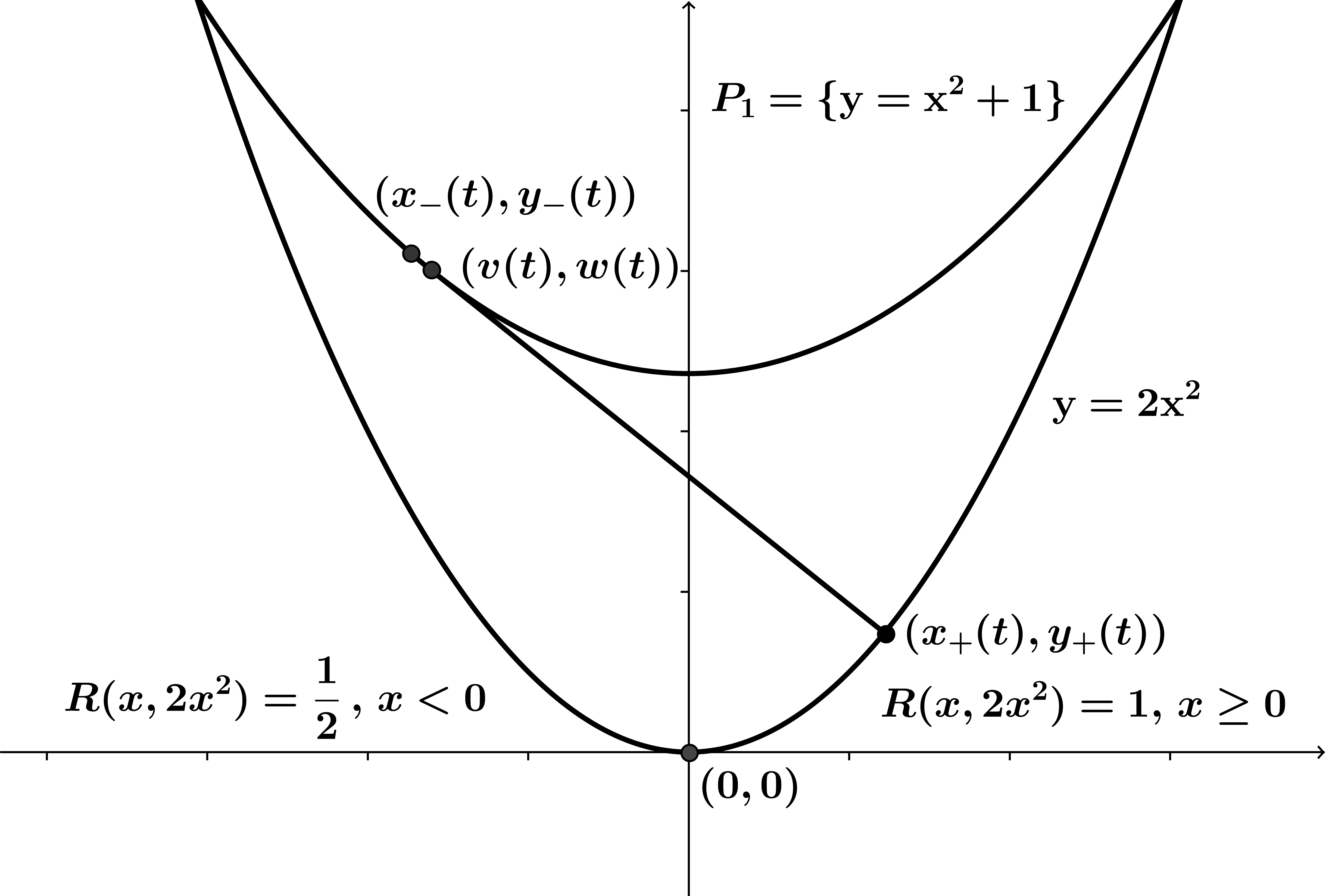
Consider a parametrization (v⁡(t),w⁡(t))(v(t),w(t)) of the arc P1P_{1}. More specifically, we consider two functions vv and w=v2+1w=v^{2}+1 defined on [1,+∞][1,+\infty] such that vv increases, v⁡(1)=−1v(1)=-1, and v⁡(+∞)=1v(+\infty)=1. We split every point (v⁡(t),w⁡(t))∈P1(v(t),w(t))\in P_{1} into (x+​(t),y+​(t))(x_{+}(t),y_{+}(t)) lying on the boundary {y=2​x2,x⩾0}\{y=2x^{2},x\geqslant 0\} and an infinitesimally close point (x−​(t),y−​(t))(x_{-}(t),y_{-}(t)), according to the rules (4.2) (see Figure 2). We will search for the function 𝐌:ωsmile→ℝ{\bf M}\colon\omega_{\mathrm{smile}}\to\mathbb{R} satisfying homogeneity relation (4.4) (with 𝐌{\bf M} instead of 𝐑{\bf R}) for which the main inequality ‘‘turns into equality’’ along the said splitting. It will appear that the function 𝐌{\bf M} constructed in such a way satisfies the equation

𝐌⁡(v,w)+⟨∇𝐌​(v,w),(x+−v,y+−w)⟩=1.{\bf M}(v,w)+\Big\langle\nabla{\bf M}\big(v,w\big),\left(x_{+}-v,y_{+}-w\right)\Big\rangle=1. (4.6)

Note that the parametrization has not been specified yet. It will be specified in Subsubsection 4.1.3 below.

The trace of 𝐌{\bf M} on P1P_{1} will be denoted by Ψ\Psi:

Ψ⁡(x)=𝐌⁡(x,x2+1),x∈[−1,1];𝐌⁡(x,y)=Ψ⁡(xy−x2),(x,y)∈ωsmile.{\Psi(x)={\bf M}(x,x^{2}+1),\quad x\in[-1,1];\qquad{\bf M}(x,y)=\Psi\Big(\frac{x}{\sqrt{y-x^{2}}}\Big),\quad(x,y)\in\omega_{\mathrm{smile}}.} (4.7)
Refer to caption
Figure 2: Illustration to the model problem

Recall the boundary values (4.3). We will search for the functions v,wv,w, and Ψ\Psi in the form

v⁡(t)=1t​∫0tφ⁡(s)​𝑑s,w⁡(t)=1t​∫0t2​φ2​(s)​𝑑s,Ψ⁡(v⁡(t))=1t​∫0th⁡(φ⁡(s))​𝑑s,t⩾1,v(t)=\frac{1}{t}\int\limits_{0}^{t}\varphi(s)\,ds,\qquad w(t)=\frac{1}{t}\int\limits_{0}^{t}2\varphi^{2}(s)\,ds,\qquad\Psi(v(t))=\frac{1}{t}\int\limits_{0}^{t}h(\varphi(s))\,ds,\qquad t\geqslant 1, (4.8)

where φ\varphi satisfies the conditions

φ:[0,∞)→ℝ,φ⁡(t)=−1​ for ​t∈[0,1);φ⁡(1)=0;φ⁡(t)⩾0​ for ​t⩾1.\varphi\colon[0,\infty)\to\mathbb{R},\qquad\varphi(t)=-1\,\text{ for }t\in[0,1);\qquad\varphi(1)=0;\qquad\varphi(t)\geqslant 0\,\text{ for }t\geqslant 1. (4.9)

We also require φ\varphi to be a non-decreasing function. One may check that x+​(t)=φ​(t)x_{+}(t)=\varphi(t), y+​(t)=2​φ2​(t)y_{+}(t)=2\varphi^{2}(t) in the sense that the tangent vector to the curve (v⁡(t),w⁡(t))(v(t),w(t)) points to (φ⁡(t),2​φ2​(t))(\varphi(t),2\varphi^{2}(t)), and

v′​(t)=−v⁡(t)t+φ⁡(t)t,w′​(t)=−w⁡(t)t+2​φ2​(t)t,\displaystyle v^{\prime}(t)=-\frac{v(t)}{t}+\frac{\varphi(t)}{t},\qquad w^{\prime}(t)=-\frac{w(t)}{t}+\frac{2\varphi^{2}(t)}{t}, (4.10)
dd​t​𝐌​(v⁡(t),w⁡(t))=−𝐌⁡(v⁡(t),w⁡(t))t+h⁡(φ⁡(t))t.\displaystyle\frac{d}{dt}{\bf M}(v(t),w(t))=-\frac{{\bf M}(v(t),w(t))}{t}+\frac{h(\varphi(t))}{t}. (4.11)

We rewrite the left hand side of (4.11):

dd​t​𝐌​(v⁡(t),w⁡(t))=⟨∇𝐌​(v⁡(t),w⁡(t)),(v′​(t),w′​(t))⟩=−1t​⟨∇𝐌​(v⁡(t),w⁡(t)),(v⁡(t)−φ⁡(t),w⁡(t)−2​φ​(t)2)⟩,\frac{d}{dt}{\bf M}(v(t),w(t))=\langle\nabla{\bf M}(v(t),w(t)),(v^{\prime}(t),w^{\prime}(t))\rangle=\\ -\frac{1}{t}\langle\nabla{\bf M}(v(t),w(t)),(v(t)-\varphi(t),w(t)-2\varphi(t)^{2})\rangle, (4.12)

then plug (4.12) into (4.11) taking into account that h⁡(φ⁡(t))=1h(\varphi(t))=1 for t⩾1t\geqslant 1, and obtain (4.6).

4.1.3 Solution of differential equation

Using (4.8) and the relation w=v2+1w=v^{2}+1, we can write down the following chain of equalities:

t⁡(v2​(t)+1)=t​w​(t)=2​∫0tφ2​(s)​𝑑s=(4.10)2​∫0t(v⁡(s)+s​v′​(s))2​𝑑s.t(v^{2}(t)+1)=tw(t)=2\int_{0}^{t}\varphi^{2}(s)\,ds\stackrel{{\scriptstyle\scriptscriptstyle\eqref{model_UVG_deriv}}}{{=}}2\int_{0}^{t}\big(v(s)+sv^{\prime}(s)\big)^{2}ds. (4.13)

We differentiate this relation and obtain

v2​(t)+1+2​t​v​(t)​v′​(t)=2​(v⁡(t)+t​v′​(t))2,v^{2}(t)+1+2tv(t)v^{\prime}(t)=2(v(t)+tv^{\prime}(t))^{2},

or

(v⁡(t)+2​t​v′​(t))2=2−v2​(t).(v(t)+2tv^{\prime}(t))^{2}=2-v^{2}(t).

We are looking for increasing functions φ\varphi and vv. Thereby, we have to solve the following Cauchy problem

2​t​v′​(t)=−v⁡(t)+2−v2​(t),v⁡(1)=−1,t⩾1,2tv^{\prime}(t)=-v(t)+\sqrt{2-v^{2}(t)},\qquad v(1)=-1,\qquad t\geqslant 1,

or

d​tt=2​d​v2−v2−v.\frac{dt}{t}=\frac{2dv}{\sqrt{2-v^{2}}-v}\,.

Hence

logt=∫−1v22−z2−zdz=∫−π/4arcsin⁡(v2)2cos⁡θ−sin⁡θcosθdθ=(θ−log(cosθ−sinθ))|−π/4arcsin⁡(v2)=arcsin(v2)+π4+log⁡22−log(1−v22−v2).\log t=\int_{-1}^{v}\frac{2}{\sqrt{2-z^{2}}-z}\,dz\;=\int_{-\pi/4}^{\arcsin(\frac{v}{\sqrt{2}})}\!\!\frac{2}{\cos\theta-\sin\theta}\cos\theta\,d\theta=\\ \Big(\theta-\log(\cos\theta-\sin\theta)\Big)\Big|_{-\pi/4}^{\arcsin(\frac{v}{\sqrt{2}})}=\arcsin\left(\frac{v}{\sqrt{2}}\right)+\frac{\pi}{4}+\frac{\log 2}{2}-\log\left(\sqrt{1-\frac{v^{2}}{2}}-\frac{v}{\sqrt{2}}\right).

Therefore,

t=22−v2−v​earcsin⁡(v2)+π4.t=\frac{2}{\sqrt{2-v^{2}}-v}\,e^{\arcsin\left(\frac{v}{\sqrt{2}}\right)+\frac{\pi}{4}}. (4.14)

Note that tt runs from 11 to +∞+\infty as vv runs from −1-1 to 11.

Now, we are able to compute Ψ⁡(v⁡(t))\Psi(v(t)). Recall that φ⁡(t)=−1\varphi(t)=-1, when t∈[0,1)t\in[0,1), and φ⁡(t)>0\varphi(t)>0 for t>1t>1. Therefore, for t∈[0,1)t\in[0,1) we have

Ψ⁡(v⁡(t))=𝐌⁡(−1,2)=12.\Psi(v(t))={\bf M}(-1,2)=\frac{1}{2}\,.

For t>1t>1 we use the last formula in (4.8) and the definition of the function hh in (4.3) and deduce

Ψ⁡(v⁡(t))=1t​∫0112​𝑑s+1t​∫1t1​𝑑s=1−12​t.\Psi(v(t))=\frac{1}{t}\int\limits_{0}^{1}\frac{1}{2}\,ds+\frac{1}{t}\int\limits_{1}^{t}1\,ds=1-\frac{1}{2t}. (4.15)

If we plug here the solution found in (4.14), we get

Ψ⁡(v)=1−2−v2−v4​e−arcsin⁡(v2)−π4,v∈[−1,1].\Psi(v)=1-\frac{\sqrt{2-v^{2}}-v}{4}e^{-\arcsin\left(\frac{v}{\sqrt{2}}\right)-\frac{\pi}{4}},\qquad v\in[-1,1]. (4.16)

By the homogeneity relation (4.7) for an arbitrary point (x,y)∈ωsmile(x,y)\in\omega_{\mathrm{smile}} we have

𝐌⁡(x,y)=1−1−ρ2−ρ2​2​e−arcsin⁡ρ−π4, where ​ρ=ρ⁡(x,y)=x2​(y−x2).{\bf M}(x,y)=1-\frac{\sqrt{1-\rho^{2}}-\rho}{2\sqrt{2}}e^{-\arcsin\rho-\frac{\pi}{4}},\quad\text{ where }\ \rho=\rho(x,y)=\frac{x}{\sqrt{2(y-x^{2})}}. (4.17)

We have finished the construction of the function 𝐌{\bf M} and now will prove that it solves the model problem.

4.1.4 Verification of the main inequality

We would like to prove that the function 𝐌{\bf M} defined in (4.17) satisfies the main inequality (4.2) of the model problem. We will not do this directly, but rather rely upon a principle similar to Lemma 2.4. We omit the proof of the following lemma because it is completely similar to the proof of Lemma 2.4.

Lemma 4.2.

Assume R:ωsmile→ℝR\colon\omega_{\mathrm{smile}}\to\mathbb{R} is differentiable on ωsmile\omega_{\mathrm{smile}} and satisfies the inequality

R⁡(x¯,y¯)⩽R⁡(x0,y0)+∂R∂x​(x0,y0)⋅(x¯−x0)+∂R∂y​(x0,y0)⋅(y¯−y0)R(\bar{x},\bar{y})\leqslant R(x_{0},y_{0})+\frac{\partial R}{\partial x}(x_{0},y_{0})\cdot(\bar{x}-x_{0})+\frac{\partial R}{\partial y}(x_{0},y_{0})\cdot(\bar{y}-y_{0}) (4.18)

for every points (x0,y0)∈ωsmile(x_{0},y_{0})\in\omega_{\mathrm{smile}} and (x¯,y¯)∈ωsmile(\bar{x},\bar{y})\in\omega_{\mathrm{smile}} such that y¯−y0=2​x0​(x¯−x0)\bar{y}-y_{0}=2x_{0}(\bar{x}-x_{0}). Then, RR satisfies the main inequality of the model problem (4.2).

Lemma 4.3.

The function 𝐌{\bf M} as in (4.17) satisfies (4.18) in the role of RR, i. e., the inequality

𝐌⁡(x¯,y¯)⩽𝐌⁡(x0,y0)+∂𝐌∂x​(x0,y0)⋅(x¯−x0)+∂𝐌∂y​(x0,y0)⋅(y¯−y0){\bf M}(\bar{x},\bar{y})\leqslant{\bf M}(x_{0},y_{0})+\frac{\partial{\bf M}}{\partial x}(x_{0},y_{0})\cdot(\bar{x}-x_{0})+\frac{\partial{\bf M}}{\partial y}(x_{0},y_{0})\cdot(\bar{y}-y_{0}) (4.19)

holds true for any (x0,y0)∈ωsmile(x_{0},y_{0})\in\omega_{\mathrm{smile}} and (x¯,y¯)∈ωsmile(\bar{x},\bar{y})\in\omega_{\mathrm{smile}} such that y¯−y0=2​x0​(x¯−x0)\bar{y}-y_{0}=2x_{0}(\bar{x}-x_{0}).

Proof.

Case x¯>x0\bar{x}>x_{0}.

Let c∈(0,1]c\in(0,1]. For any point (x,y)(x,y) such that (x,y)∈ωsmile(x,y)\in\omega_{\mathrm{smile}} and max⁡(−2​c​x,x2)⩽y⩽x2+c2\max(-2cx,x^{2})\leqslant y\leqslant x^{2}+c^{2} we find two numbers uRu_{{}_{\mathrm{R}}} and vRv_{{}_{\mathrm{R}}} such that vR⩽x⩽uRv_{{}_{\mathrm{R}}}\leqslant x\leqslant u_{{}_{\mathrm{R}}} and

2uR2−vR2−c2uR−vR=y−vR2−c2x−vR=2vR,\frac{2u_{{}_{\mathrm{R}}}^{2}-v_{{}_{\mathrm{R}}}^{2}-c^{2}}{u_{{}_{\mathrm{R}}}-v_{{}_{\mathrm{R}}}}=\frac{y-v_{{}_{\mathrm{R}}}^{2}-c^{2}}{x-v_{{}_{\mathrm{R}}}}=2v_{{}_{\mathrm{R}}},

see Figure 3.

Refer to caption
Figure 3: Definition of uRu_{{}_{\mathrm{R}}} and vRv_{{}_{\mathrm{R}}}.

We deduce that

vR=vR(x,y,c)=x−x2+c2−y,uR=uR(x,y,c)=vR+2c2−vR22.v_{{}_{\mathrm{R}}}=v_{{}_{\mathrm{R}}}(x,y,c)=x-\sqrt{x^{2}+c^{2}-y},\qquad u_{{}_{\mathrm{R}}}=u_{{}_{\mathrm{R}}}(x,y,c)=\frac{v_{{}_{\mathrm{R}}}+\sqrt{2c^{2}-v_{{}_{\mathrm{R}}}^{2}}}{2}. (4.20)

We introduce the function GRG_{{}_{\mathrm{R}}} defined on the domain

{(x,y,c)|c∈(0,1],max(−2cx,x2)⩽y⩽x2+c2}\Big\{(x,y,c)\,\Big|\;c\in(0,1],\,\max(-2cx,x^{2})\leqslant y\leqslant x^{2}+c^{2}\Big\}

by the formula:

GR(x,y,c)=uR−xuR−vRΨ(vRc)+x−vRuR−vR=uR−xuR−vR(Ψ(vRc)−1)+1,G_{{}_{\mathrm{R}}}(x,y,c)=\frac{u_{{}_{\mathrm{R}}}-x}{u_{{}_{\mathrm{R}}}-v_{{}_{\mathrm{R}}}}\Psi\left(\frac{v_{{}_{\mathrm{R}}}}{c}\right)+\frac{x-v_{{}_{\mathrm{R}}}}{u_{{}_{\mathrm{R}}}-v_{{}_{\mathrm{R}}}}=\frac{u_{{}_{\mathrm{R}}}-x}{u_{{}_{\mathrm{R}}}-v_{{}_{\mathrm{R}}}}\left(\Psi\left(\frac{v_{{}_{\mathrm{R}}}}{c}\right)-1\right)+1, (4.21)

where uR=uR(x,y,c)u_{{}_{\mathrm{R}}}=u_{{}_{\mathrm{R}}}(x,y,c), vR=vR(x,y,c)v_{{}_{\mathrm{R}}}=v_{{}_{\mathrm{R}}}(x,y,c), and Ψ\Psi was defined in (4.7) and got its explicit form in (4.16). For any cc fixed the function GR(⋅,⋅,c)G_{{}_{\mathrm{R}}}(\,\cdot\,,\,\cdot\,,c) is linear along each segment connecting the points (vR,vR2+c2)(v_{{}_{\mathrm{R}}},v_{{}_{\mathrm{R}}}^{2}+c^{2}) and (uR,2uR2)(u_{{}_{\mathrm{R}}},2u_{{}_{\mathrm{R}}}^{2}), and coincides with 𝐌{\bf M} at their endpoints. Also from the construction of 𝐌{\bf M} (see formula (4.6)) we deduce that the function GRG_{{}_{\mathrm{R}}} has the following property:

𝐌(x0,y0)+∂𝐌∂x(x0,y0)⋅(x¯−x0)+∂𝐌∂y(x0,y0)⋅2x0(x¯−x0)=GR(x¯,y¯,c0){\bf M}(x_{0},y_{0})+\frac{\partial{\bf M}}{\partial x}(x_{0},y_{0})\cdot(\bar{x}-x_{0})+\frac{\partial{\bf M}}{\partial y}(x_{0},y_{0})\cdot 2x_{0}(\bar{x}-x_{0})=G_{{}_{\mathrm{R}}}(\bar{x},\bar{y},c_{0}) (4.22)

with c0=y0−x02c_{0}=\sqrt{y_{0}-x_{0}^{2}}.

On the other hand, for c¯=y¯−x¯2\bar{c}=\sqrt{\bar{y}-\bar{x}^{2}} we have vR(x¯,y¯,c¯)=x¯v_{{}_{\mathrm{R}}}(\bar{x},\bar{y},\bar{c})=\bar{x}, and therefore GR(x¯,y¯,c¯)=𝐌(x¯,y¯)G_{{}_{\mathrm{R}}}(\bar{x},\bar{y},\bar{c})={\bf M}(\bar{x},\bar{y}). It may be seen that c¯<c0\bar{c}<c_{0}:

c¯2=y¯−x¯2=y0−x02−(x¯−x0)2<y0−x02=c02.\bar{c}^{2}=\bar{y}-\bar{x}^{2}=y_{0}-x_{0}^{2}-(\bar{x}-x_{0})^{2}<y_{0}-x_{0}^{2}=c_{0}^{2}\,.

Thus, to prove (4.19) it suffices to show that the function GR(x¯,y¯,c)G_{{}_{\mathrm{R}}}(\bar{x},\bar{y},c) does not decrease in cc. In other words, we wish to verify the inequality

∂GR(x,y,c)∂c⩾0.\frac{\partial G_{{}_{\mathrm{R}}}(x,y,c)}{\partial c}\geqslant 0. (4.23)

It follows from (4.20) that

∂vR∂c=−cx2+c2−y=cvR−x,\frac{\partial v_{{}_{\mathrm{R}}}}{\partial c}=-\frac{c}{\sqrt{x^{2}+c^{2}-y}}=\frac{c}{v_{{}_{\mathrm{R}}}-x}, (4.24)
∂uR∂c=12​(∂vR∂c+4c−2vR∂vR∂c2​2c2−vR2)=12​(cvR−x+2​c−cvRvR−x2uR−vR)=c(uR−x)(vR−x)(2uR−vR).\frac{\partial u_{{}_{\mathrm{R}}}}{\partial c}=\frac{1}{2}\left(\frac{\partial v_{{}_{\mathrm{R}}}}{\partial c}+\frac{4c-2v_{{}_{\mathrm{R}}}\frac{\partial v_{{}_{\mathrm{R}}}}{\partial c}}{2\sqrt{2c^{2}-v_{{}_{\mathrm{R}}}^{2}}}\right)=\frac{1}{2}\left(\frac{c}{v_{{}_{\mathrm{R}}}-x}+\frac{2c-\frac{cv_{{}_{\mathrm{R}}}}{v_{{}_{\mathrm{R}}}-x}}{2u_{{}_{\mathrm{R}}}-v_{{}_{\mathrm{R}}}}\right)=\frac{c(u_{{}_{\mathrm{R}}}-x)}{(v_{{}_{\mathrm{R}}}-x)(2u_{{}_{\mathrm{R}}}-v_{{}_{\mathrm{R}}})}. (4.25)

We differentiate (4.21) and obtain

∂GR(x,y,c)∂c=∂uR∂c(uR−vR)−(∂uR∂c−∂vR∂c)(uR−x)(uR−vR)2​(Ψ⁡(vRc)−1)+uR−xuR−vR⋅∂vR∂cc−vRc2​Ψ′​(vRc).\frac{\partial G_{{}_{\mathrm{R}}}(x,y,c)}{\partial c}=\frac{\frac{\partial u_{{}_{\mathrm{R}}}}{\partial c}(u_{{}_{\mathrm{R}}}-v_{{}_{\mathrm{R}}})-(\frac{\partial u_{{}_{\mathrm{R}}}}{\partial c}-\frac{\partial v_{{}_{\mathrm{R}}}}{\partial c})(u_{{}_{\mathrm{R}}}-x)}{(u_{{}_{\mathrm{R}}}-v_{{}_{\mathrm{R}}})^{2}}\left(\Psi\left(\frac{v_{{}_{\mathrm{R}}}}{c}\right)-1\right)+\frac{u_{{}_{\mathrm{R}}}-x}{u_{{}_{\mathrm{R}}}-v_{{}_{\mathrm{R}}}}\cdot\frac{\frac{\partial v_{{}_{\mathrm{R}}}}{\partial c}c-v_{{}_{\mathrm{R}}}}{c^{2}}\Psi^{\prime}\left(\frac{v_{{}_{\mathrm{R}}}}{c}\right).

Formula (4.16) for the function Ψ\Psi implies

Ψ′(v)=12e−π/4−arcsinv2.\Psi^{\prime}(v)=\frac{1}{2}e^{-\pi/4-\arcsin\frac{v}{\sqrt{2}}}. (4.26)

Using (4.16) and (4.26), we continue the evaluation of ∂GR(x,y,c)∂c\frac{\partial G_{{}_{\mathrm{R}}}(x,y,c)}{\partial c} and obtain that it equals to

(∂uR∂c(uR−vR−uR+x)+∂vR∂c(uR−x)4(uR−vR)2​(vRc−2−vR2c2)+uR−xuR−vR⋅∂vR∂cc−vR2​c2)​e−arcsin⁡(vR2​c)−π4.\left(\frac{\frac{\partial u_{{}_{\mathrm{R}}}}{\partial c}(u_{{}_{\mathrm{R}}}-v_{{}_{\mathrm{R}}}-u_{{}_{\mathrm{R}}}+x)+\frac{\partial v_{{}_{\mathrm{R}}}}{\partial c}(u_{{}_{\mathrm{R}}}-x)}{4(u_{{}_{\mathrm{R}}}-v_{{}_{\mathrm{R}}})^{2}}\left(\frac{v_{{}_{\mathrm{R}}}}{c}-\sqrt{2-\frac{v_{{}_{\mathrm{R}}}^{2}}{c^{2}}}\right)+\frac{u_{{}_{\mathrm{R}}}-x}{u_{{}_{\mathrm{R}}}-v_{{}_{\mathrm{R}}}}\cdot\frac{\frac{\partial v_{{}_{\mathrm{R}}}}{\partial c}c-v_{{}_{\mathrm{R}}}}{2c^{2}}\right)e^{-\arcsin\big(\frac{v_{{}_{\mathrm{R}}}}{\sqrt{2}c}\big)-\frac{\pi}{4}}.

We may omit the exponent multiplier since we are interested in the sign of the expression ∂GR(x,y,c)∂c\frac{\partial G_{{}_{\mathrm{R}}}(x,y,c)}{\partial c} only. Note that relation (4.20) yields

vRc−2−vR2c2=2​vR−uRc.\frac{v_{{}_{\mathrm{R}}}}{c}-\sqrt{2-\frac{v_{{}_{\mathrm{R}}}^{2}}{c^{2}}}=2\frac{v_{R}-u_{R}}{c}.

Applying (4.24) and (4.25), we continue the computation

1(uR−vR)2\displaystyle\frac{1}{(u_{{}_{\mathrm{R}}}-v_{{}_{\mathrm{R}}})^{2}} ((x−vR)c(uR−x)(vR−x)(2uR−vR)+c(uR−x)vR−x)2(vR−uR)4​c+uR−x2c2(uR−vR)(c2vR−x−vR)\displaystyle\left((x-v_{{}_{\mathrm{R}}})\frac{c(u_{{}_{\mathrm{R}}}-x)}{(v_{{}_{\mathrm{R}}}-x)(2u_{{}_{\mathrm{R}}}-v_{{}_{\mathrm{R}}})}+\frac{c(u_{{}_{\mathrm{R}}}-x)}{v_{{}_{\mathrm{R}}}-x}\right)\frac{2(v_{{}_{\mathrm{R}}}-u_{{}_{\mathrm{R}}})}{4c}+\frac{u_{{}_{\mathrm{R}}}-x}{2c^{2}(u_{{}_{\mathrm{R}}}-v_{{}_{\mathrm{R}}})}\left(\frac{c^{2}}{v_{{}_{\mathrm{R}}}-x}-v_{{}_{\mathrm{R}}}\right)
=uR−x2(uR−vR)2(1vR−2uR+1vR−x)(vR−uR)−uR−x2(vR−uR)(1vR−x−vRc2)\displaystyle=\rule{0.0pt}{22.0pt}\frac{u_{{}_{\mathrm{R}}}-x}{2(u_{{}_{\mathrm{R}}}-v_{{}_{\mathrm{R}}})^{2}}\left(\frac{1}{v_{{}_{\mathrm{R}}}-2u_{{}_{\mathrm{R}}}}+\frac{1}{v_{{}_{\mathrm{R}}}-x}\right)(v_{{}_{\mathrm{R}}}-u_{{}_{\mathrm{R}}})-\frac{u_{{}_{\mathrm{R}}}-x}{2(v_{{}_{\mathrm{R}}}-u_{{}_{\mathrm{R}}})}\left(\frac{1}{v_{{}_{\mathrm{R}}}-x}-\frac{v_{{}_{\mathrm{R}}}}{c^{2}}\right)
=uR−x2(vR−uR)(1vR−2uR+vRc2)=uR−x2c2(uR−vR)(2uR−vR)((vR−uR)2+c2−uR2),\displaystyle=\rule{0.0pt}{22.0pt}\frac{u_{{}_{\mathrm{R}}}-x}{2(v_{{}_{\mathrm{R}}}-u_{{}_{\mathrm{R}}})}\left(\frac{1}{v_{{}_{\mathrm{R}}}-2u_{{}_{\mathrm{R}}}}+\frac{v_{{}_{\mathrm{R}}}}{c^{2}}\right)=\frac{u_{{}_{\mathrm{R}}}-x}{2c^{2}(u_{{}_{\mathrm{R}}}-v_{{}_{\mathrm{R}}})(2u_{{}_{\mathrm{R}}}-v_{{}_{\mathrm{R}}})}\big((v_{{}_{\mathrm{R}}}-u_{{}_{\mathrm{R}}})^{2}+c^{2}-u_{{}_{\mathrm{R}}}^{2}\big),

which is non-negative because 0⩽uR⩽c0\leqslant u_{{}_{\mathrm{R}}}\leqslant c and vR⩽x⩽uRv_{{}_{\mathrm{R}}}\leqslant x\leqslant u_{{}_{\mathrm{R}}}. This finishes the proof of (4.23).

Case x¯<x0\bar{x}<x_{0}.

We will construct another auxiliary function GLG_{{}_{\mathrm{L}}} in the following way. Let c>0c>0. For any point (x,y)(x,y) such that (x,y)∈ωsmile(x,y)\in\omega_{\mathrm{smile}} and max⁡(2​c​x,x2)⩽y⩽x2+c2\max(2cx,x^{2})\leqslant y\leqslant x^{2}+c^{2}, we find two numbers uLu_{{}_{\mathrm{L}}} and vLv_{{}_{\mathrm{L}}} such that x⩽vL⩽uLx\leqslant v_{{}_{\mathrm{L}}}\leqslant u_{{}_{\mathrm{L}}} and

2uL2−vL2−c2uL−vL=y−vL2−c2x−vL=2vL,\frac{2u_{{}_{\mathrm{L}}}^{2}-v_{{}_{\mathrm{L}}}^{2}-c^{2}}{u_{{}_{\mathrm{L}}}-v_{{}_{\mathrm{L}}}}=\frac{y-v_{{}_{\mathrm{L}}}^{2}-c^{2}}{x-v_{{}_{\mathrm{L}}}}=2v_{{}_{\mathrm{L}}},

see Figure 4.

Refer to caption
Figure 4: Definition of uLu_{{}_{\mathrm{L}}} and vLv_{{}_{\mathrm{L}}}.

After some calculations, we get

vL=vL(x,y,c)=x+x2+c2−y,uL=uL(x,y,c)=vL+2c2−vL22.v_{{}_{\mathrm{L}}}=v_{{}_{\mathrm{L}}}(x,y,c)=x+\sqrt{x^{2}+c^{2}-y},\qquad u_{{}_{\mathrm{L}}}=u_{{}_{\mathrm{L}}}(x,y,c)=\frac{v_{{}_{\mathrm{L}}}+\sqrt{2c^{2}-v_{{}_{\mathrm{L}}}^{2}}}{2}. (4.27)

We introduce the function GLG_{{}_{\mathrm{L}}} defined on the domain

{(x,y,c)|c∈(0,1],max(2cx,x2)⩽y⩽x2+c2}\Big\{(x,y,c)\,\Big|\;c\in(0,1],\,\max(2cx,x^{2})\leqslant y\leqslant x^{2}+c^{2}\Big\}

by the formula:

GL(x,y,c)=uL−xuL−vLΨ(vLc)+x−vLuL−vL=uL−xuL−vL(Ψ(vLc)−1)+1.G_{{}_{\mathrm{L}}}(x,y,c)=\frac{u_{{}_{\mathrm{L}}}-x}{u_{{}_{\mathrm{L}}}-v_{{}_{\mathrm{L}}}}\Psi\left(\frac{v_{{}_{\mathrm{L}}}}{c}\right)+\frac{x-v_{{}_{\mathrm{L}}}}{u_{{}_{\mathrm{L}}}-v_{{}_{\mathrm{L}}}}=\frac{u_{{}_{\mathrm{L}}}-x}{u_{{}_{\mathrm{L}}}-v_{{}_{\mathrm{L}}}}\left(\Psi\left(\frac{v_{{}_{\mathrm{L}}}}{c}\right)-1\right)+1. (4.28)

For any cc fixed the function GL(⋅,⋅,c)G_{{}_{\mathrm{L}}}(\,\cdot\,,\,\cdot\,,c) is linear on the extension of the segment connecting the points (vL,vL2+c2)(v_{{}_{\mathrm{L}}},v_{{}_{\mathrm{L}}}^{2}+c^{2}) and (uL,2uL2)(u_{{}_{\mathrm{L}}},2u_{{}_{\mathrm{L}}}^{2}) beyond the point (vL,vL2+c2)(v_{{}_{\mathrm{L}}},v_{{}_{\mathrm{L}}}^{2}+c^{2}), and coincides with 𝐌{\bf M} at these two points. Also from the construction of 𝐌{\bf M} (see (4.6)) we deduce that the function GLG_{{}_{\mathrm{L}}} satisfies the following property:

𝐌(x0,y0)+∂𝐌∂x(x0,y0)⋅(x¯−x0)+∂𝐌∂y(x0,y0)⋅2x0(x¯−x0)=GL(x¯,y¯,c0),{\bf M}(x_{0},y_{0})+\frac{\partial{\bf M}}{\partial x}(x_{0},y_{0})\cdot(\bar{x}-x_{0})+\frac{\partial{\bf M}}{\partial y}(x_{0},y_{0})\cdot 2x_{0}(\bar{x}-x_{0})=G_{{}_{\mathrm{L}}}(\bar{x},\bar{y},c_{0}), (4.29)

for c0=y0−x02c_{0}=\sqrt{y_{0}-x_{0}^{2}}.

On the other hand, for c¯=y¯−x¯2\bar{c}=\sqrt{\bar{y}-\bar{x}^{2}} we have GL(x¯,y¯,c¯)=𝐌(x¯,y¯)G_{{}_{\mathrm{L}}}(\bar{x},\bar{y},\bar{c})={\bf M}(\bar{x},\bar{y}). Again, we have c¯<c0\bar{c}<c_{0}. Thus, it suffices to show that the function GL(x¯,y¯,c)G_{{}_{\mathrm{L}}}(\bar{x},\bar{y},c) increases in cc, i. e., the inequality

∂GL(x,y,c)∂c⩾0.\frac{\partial G_{{}_{\mathrm{L}}}(x,y,c)}{\partial c}\geqslant 0. (4.30)

From equations (4.27) we obtain

∂vL∂c=cx2+c2−y=cvL−x.\frac{\partial v_{{}_{\mathrm{L}}}}{\partial c}=\frac{c}{\sqrt{x^{2}+c^{2}-y}}=\frac{c}{v_{{}_{\mathrm{L}}}-x}\,. (4.31)

We note that the right hand side of (4.31) coincides with the right hand side of (4.24) (vRv_{{}_{\mathrm{R}}} is simply replaced with vLv_{{}_{\mathrm{L}}}), and uLu_{{}_{\mathrm{L}}} is defined by vLv_{{}_{\mathrm{L}}} exactly in the same way as uRu_{{}_{\mathrm{R}}} was defined by vRv_{{}_{\mathrm{R}}}. The same calculations as we have already done in the proof of (4.23) lead us to the fact that (4.30) is equivalent to

uL−xc2(uL−vL)(2uL−vL)((vL−uL)2+c2−uL2)⩾0,\frac{u_{{}_{\mathrm{L}}}-x}{c^{2}(u_{{}_{\mathrm{L}}}-v_{{}_{\mathrm{L}}})(2u_{{}_{\mathrm{L}}}-v_{{}_{\mathrm{L}}})}\big((v_{{}_{\mathrm{L}}}-u_{{}_{\mathrm{L}}})^{2}+c^{2}-u_{{}_{\mathrm{L}}}^{2}\big)\geqslant 0, (4.32)

which holds true because x⩽vL⩽uLx\leqslant v_{{}_{\mathrm{L}}}\leqslant u_{{}_{\mathrm{L}}} and 0⩽uL⩽c0\leqslant u_{{}_{\mathrm{L}}}\leqslant c. ∎

4.1.5 Minimality

Lemmas 4.2 and 4.3 imply 𝐌⁡(x,y)⩾𝐑⁡(x,y){\bf M}(x,y)\geqslant{\bf R}(x,y) for any (x,y)∈ωsmile(x,y)\in\omega_{\mathrm{smile}}. Now we wish to prove the reverse inequality.

Lemma 4.4.

Let 𝐑{\bf R} be the solution of the model problem and let 𝐌{\bf M} be the function defined in (4.17). Then, for any (x,y)∈ωsmile,(x,y)\in\omega_{\mathrm{smile}}, we have 𝐑⁡(x,y)⩾𝐌⁡(x,y){\bf R}(x,y)\geqslant{\bf M}(x,y).

Proof.

Due to the homogeneity relation (4.4), it suffices to consider the case (x,y)∈P1(x,y)\in P_{1}. Let 𝐫⁡(t)=𝐑⁡(v⁡(t),w⁡(t)){\bf r}(t)={\bf R}(v(t),w(t)), here we use the parametrization (v⁡(t),w⁡(t))(v(t),w(t)) of P1P_{1} introduced in Subsubsection 4.1.2. We will show that 𝐫{\bf r} is continuous and for every t⩾1t\geqslant 1 the inequality

d−d​t​[t​𝐫​(t)]⩾1\frac{d_{-}}{dt}[t\ {\bf r}(t)]\geqslant 1 (4.33)

holds true. By d−d​t\frac{\ d_{-}}{dt} we mean the lower derivative, that is

d−​rd​t​(t0)=lim inft→t0r⁡(t)−r⁡(t0)t−t0.\frac{d_{-}r}{dt}(t_{0})=\liminf\limits_{t\to t_{0}}\frac{r(t)-r(t_{0})}{t-t_{0}}.

Once (4.33) is proved, we may use formula (4.15) that implies

d−d​t​[t⁡(𝐫⁡(v⁡(t))−Ψ⁡(v⁡(t)))]⩾0.{\frac{d_{-}}{dt}\left[t\Big({\bf r}(v(t))-\Psi(v(t))\Big)\right]\geqslant 0.} (4.34)

This yields the desired estimate 𝐑⁡(v⁡(t),w⁡(t))−𝐌⁡(v⁡(t),w⁡(t))⩾0{\bf R}(v(t),w(t))-{\bf M}(v(t),w(t))\geqslant 0, because the two functions in question are continuous and are equal at t=1t=1.

The proof of (4.33) and the continuity of 𝐫{\bf r} will take some time. Fix a point (v0,w0)(v_{0},w_{0}), where w0=v02+1w_{0}=v_{0}^{2}+1 and v0=v⁡(t0)v_{0}=v(t_{0}) for some t0∈(1,∞)t_{0}\in(1,\infty). Draw the tangent line through (v0,w0)(v_{0},w_{0}) to the upper boundary of ωsmile\omega_{\mathrm{smile}}:

y=2​v0​x+1−v02.{y=2v_{0}x+1-v_{0}^{2}.} (4.35)

Take two more points on this line (x±,y±)(x_{\pm},y_{\pm}), where one of them is the right point of intersection with the lower boundary of ωsmile\omega_{\mathrm{smile}}, i. e.,

x+=φ⁡(t0)=v0+2−v022,y+=2​φ2​(t0)=1+v0​2−v02,x_{+}=\varphi(t_{0})=\frac{v_{0}+\sqrt{2-v_{0}^{2}}}{2}\,,\qquad y_{+}=2\varphi^{2}(t_{0})=1+v_{0}\sqrt{2-v_{0}^{2}}\,,

and the second is defined as follows:

x−=v​v0+1+v2−v021+v2​v,y−=(v​v0+1+v2−v02)21+v2,x_{-}=\frac{vv_{0}+\sqrt{1+v^{2}-v_{0}^{2}}}{1+v^{2}}v\,,\qquad y_{-}=\frac{\big(vv_{0}+\sqrt{1+v^{2}-v_{0}^{2}}\big)^{2}}{1+v^{2}}, (4.36)

where v=v⁡(t)v=v(t) for some t∈[1,∞)t\in[1,\infty), t≠t0t\neq t_{0}. At these points we have 𝐑⁡(x+,y+)=1{\bf R}(x_{+},y_{+})=1 and 𝐑⁡(x−,y−)=𝐫⁡(t){\bf R}(x_{-},y_{-})={\bf r}(t). The latter identity holds true by (4.4), because the points (x−,y−)(x_{-},y_{-}) and (v,v2+1)(v,v^{2}+1) lie on the parabola

y=1+v2v2​x2.y=\frac{1+v^{2}}{v^{2}}x^{2}.

We write down the concavity property (4.2):

𝐫⁡(t0)⩾x+−v0x+−x−⋅𝐫⁡(t)+v0−x−x+−x−⋅1,\displaystyle{\bf r}(t_{0})\geqslant\frac{x_{+}-v_{0}}{x_{+}-x_{-}}\cdot{\bf r}(t)+\frac{v_{0}-x_{-}}{x_{+}-x_{-}}\cdot 1, if ​t<t0;\displaystyle\qquad\text{if }\ t<t_{0}\,; (4.37)
𝐫⁡(t)⩾x+−x−x+−v0⋅𝐫⁡(t0)+x−−v0x+−v0⋅1,\displaystyle{\bf r}(t)\geqslant\frac{x_{+}-x_{-}}{x_{+}-v_{0}}\cdot{\bf r}(t_{0})+\frac{x_{-}-v_{0}}{x_{+}-v_{0}}\cdot 1, if ​t>t0.\displaystyle\qquad\text{if }\ t>t_{0}\,. (4.38)

We may rewrite (4.37) and (4.38) as follows

(x+−v0)​(𝐫⁡(t)−𝐫⁡(t0))⩽(x−−v0)​(1−𝐫⁡(t0)),\displaystyle(x_{+}-v_{0})({\bf r}(t)-{\bf r}(t_{0}))\leqslant(x_{-}-v_{0})(1-{\bf r}(t_{0})), if ​t<t0;\displaystyle\qquad\text{if }\ t<t_{0}\,;
(x+−v0)​(𝐫⁡(t)−𝐫⁡(t0))⩾(x−−v0)​(1−𝐫⁡(t0)),\displaystyle(x_{+}-v_{0})({\bf r}(t)-{\bf r}(t_{0}))\geqslant(x_{-}-v_{0})(1-{\bf r}(t_{0})), if ​t>t0.\displaystyle\qquad\text{if }\ t>t_{0}\,.

Both these inequalities turn into

𝐫⁡(t)−𝐫⁡(t0)t−t0⩾x−−v0t−t0⋅1−𝐫⁡(t0)x+−v0\frac{{\bf r}(t)-{\bf r}(t_{0})}{t-t_{0}}\geqslant\frac{x_{-}-v_{0}}{t-t_{0}}\cdot\frac{1-{\bf r}(t_{0})}{x_{+}-v_{0}} (4.39)

after dividing by (t−t0)​(x+−v0)(t-t_{0})(x_{+}-v_{0}).

Let us calculate the right hand side of this inequality. Using (4.10) we get

x+−v0=φ⁡(t0)−v⁡(t0)=t0​v′​(t0).x_{+}-v_{0}=\varphi(t_{0})-v(t_{0})=t_{0}v^{\prime}(t_{0})\,.

From the definition (4.36) of x−x_{-} we deduce

x−−v0=v2−v02v0+v​1+v2−v02.x_{-}-v_{0}=\frac{v^{2}-v_{0}^{2}}{v_{0}+v\sqrt{1+v^{2}-v_{0}^{2}}}\,.

Therefore, (4.39) may be rewritten as

𝐫⁡(t)−𝐫⁡(t0)t−t0⩾v−v0t−t0⋅v+v0v0+v​1+v2−v02⋅1−𝐫⁡(t0)t0​v′​(t0).{\frac{{\bf r}(t)-{\bf r}(t_{0})}{t-t_{0}}\geqslant\frac{v-v_{0}}{t-t_{0}}\cdot\frac{v+v_{0}}{v_{0}+v\sqrt{1+v^{2}-v_{0}^{2}}}\cdot\frac{1-{\bf r}(t_{0})}{t_{0}v^{\prime}(t_{0})}\,.} (4.40)

We see that the right hand side has a limit as t→t0t\to t_{0}:

limt→t0v−v0t−t0⋅v+v0v0+v​1+v2−v02⋅1−𝐫⁡(t0)t0​v′​(t0)=1−𝐫⁡(t0)t0,\lim_{t\to t_{0}}\frac{v-v_{0}}{t-t_{0}}\cdot\frac{v+v_{0}}{v_{0}+v\sqrt{1+v^{2}-v_{0}^{2}}}\cdot\frac{1-{\bf r}(t_{0})}{t_{0}v^{\prime}(t_{0})}=\frac{1-{\bf r}(t_{0})}{t_{0}}\,,

whence

lim inft→t0𝐫⁡(t)−𝐫⁡(t0)t−t0⩾1−𝐫⁡(t0)t0,\liminf_{t\to t_{0}}\frac{{\bf r}(t)-{\bf r}(t_{0})}{t-t_{0}}\geqslant\frac{1-{\bf r}(t_{0})}{t_{0}}\,,

what is exactly the desired estimate (4.33).

It remains to check continuity of 𝐫{\bf r}. First we note that (4.40) implies that 𝐫{\bf r} is an increasing function because vv is. We will write down the same property (4.2) with (x+,y+)(x_{+},y_{+}) being not the right but the left point of intersection with the lower boundary of ωsmile\omega_{\mathrm{smile}}, i. e.,

x+=v0−2−v022.x_{+}=\frac{v_{0}-\sqrt{2-v_{0}^{2}}}{2}.

The point (x−,y−)(x_{-},y_{-}) is defined as before by (4.36), where v=v⁡(t)v=v(t) and t>t0t>t_{0}. Thus, now we have x+<v0<x−x_{+}<v_{0}<x_{-}, 𝐑⁡(x+,y+)=12{\bf R}(x_{+},y_{+})=\tfrac{1}{2}, 𝐑⁡(x−,y−)=𝐫⁡(t){\bf R}(x_{-},y_{-})={\bf r}(t), and the concavity property (4.2) takes the form

𝐫⁡(t0)⩾x−−v0x−−x+⋅12+v0−x+x−−x+⋅𝐫⁡(t).{\bf r}(t_{0})\geqslant\frac{x_{-}-v_{0}}{x_{-}-x_{+}}\cdot\tfrac{1}{2}+\frac{v_{0}-x_{+}}{x_{-}-x_{+}}\cdot{\bf r}(t)\,.

Therefore,

(x−−v0)​(𝐫⁡(t0)−12)⩾(v0−x+)​(𝐫⁡(t)−𝐫⁡(t0)),{(x_{-}-v_{0})({\bf r}(t_{0})-\tfrac{1}{2})\geqslant(v_{0}-x_{+})({\bf r}(t)-{\bf r}(t_{0}))\,,} (4.41)

whence

0⩽𝐫⁡(t)−𝐫⁡(t0)\displaystyle 0\leqslant{\bf r}(t)-{\bf r}(t_{0}) ⩽x−−v0v0−x+​(𝐫⁡(t0)−12)⩽x−−v0v0−x+⋅12\displaystyle\leqslant\frac{x_{-}-v_{0}}{v_{0}-x_{+}}({\bf r}(t_{0})-\tfrac{1}{2})\leqslant\frac{x_{-}-v_{0}}{v_{0}-x_{+}}\cdot\tfrac{1}{2}
=v2−v02v0+v​1+v2−v02⋅1v0+2−v02⩽v−v0v0+2−v02.\displaystyle=\frac{v^{2}-v_{0}^{2}}{v_{0}+v\sqrt{1+v^{2}-v_{0}^{2}}}\cdot\frac{1}{v_{0}+\sqrt{2-v_{0}^{2}}}\leqslant\frac{v-v_{0}}{v_{0}+\sqrt{2-v_{0}^{2}}}.

Since vv is a continuous function, this inequality proves that 𝐫{\bf r} is continuous at any point t0t_{0}, t0>1t_{0}>1 (i. e., v0>−1v_{0}>-1). It remains to verify continuity of the function 𝐫{\bf r} at the point t=1t=1 from the right. We know that 𝐫{\bf r} is an increasing function, therefore, there exists a limit

limt→1+𝐫⁡(t)=def𝐫1.{\lim_{t\to 1+}{\bf r}(t)\mathrel{\mathop{\kern 0.0pt=}\limits^{\mathrm{def}}}{\bf r}_{1}.} (4.42)

Due to (4.41) we have 𝐫⁡(t0)⩾12{\bf r}(t_{0})\geqslant\tfrac{1}{2} for every t0>1t_{0}>1, whence 𝐫1⩾12{\bf r}_{1}\geqslant\tfrac{1}{2}. At the same time we have already proved that 𝐫⁡(t)⩽Ψ⁡(v⁡(t))=1−12​t{\bf r}(t)\leqslant\Psi(v(t))=1-\tfrac{1}{2t}, i. e., 𝐫1⩽12{\bf r}_{1}\leqslant\tfrac{1}{2}. So, 𝐫1=12{\bf r}_{1}=\tfrac{1}{2} and we have proved continuity of 𝐫{\bf r} on [1,∞)[1,\infty). ∎

Summarizing all preceding consideration, we conclude that the solution of the model problem is given by the following formula:

𝐑⁡(x,y)=1−1−ρ2−ρ2​2​e−arcsin⁡ρ−π4, where ​ρ=ρ⁡(x,y)=x2​(y−x2).{\bf R}(x,y)=1-\frac{\sqrt{1-\rho^{2}}-\rho}{2\sqrt{2}}e^{-\arcsin\rho-\frac{\pi}{4}},\quad\text{ where }\ \rho=\rho(x,y)=\frac{x}{\sqrt{2(y-x^{2})}}. (4.43)

4.2 Construction of the function and verification of the main inequality

The set ΩR\Omega_{R} defined in (1.19) has special relationship with the splitting rules (2.1). It follows from Lemma 2.3 that if (x,y,z)∈ΩR(x,y,z)\in\Omega_{R} is split into some points (xj,yj,zj)(x_{j},y_{j},z_{j}) according to the rules (2.1), then, first, all the points (xj,yj)(x_{j},y_{j}) lie on the tangent line to the parabola 𝐲−𝐱2=1−z2{\bf y}-{\bf x}^{2}=1-z^{2}, and second, all the points (xj,yj,zj)(x_{j},y_{j},z_{j}) belong to ΩR\Omega_{R}. One may say that ΩR\Omega_{R} has separate dynamics.

Thus, if we denote 𝑩⁡(x,y,1−y+x2)\boldsymbol{B}(x,y,\sqrt{1-y+x^{2}}) by B^​(x,y)\widehat{B}(x,y), then B^\widehat{B} may be described as the minimal among functions G:ω1→ℝG\colon\omega_{1}\to\mathbb{R} that satisfy the boundary conditions G(x,x2)=χ[0,∞)(x)G(x,x^{2})=\chi_{{}_{[0,\infty)}}(x) and the main inequality

G⁡(x,y)⩾∑j=1Nαj​G​(xj,yj),wherex=∑j=1Nαjxj,y=∑j=1Nαjyj,yj−yxj−x=2x,∑j=1Nαj=1,αj⩾0,and(x,y),(xj,yj)∈ω1.\begin{gathered}G(x,y)\geqslant\sum\limits_{j=1}^{N}\alpha_{j}G(x_{j},y_{j}),\quad\text{where}\\ x=\sum\limits_{j=1}^{N}\alpha_{j}x_{j},\qquad y=\sum\limits_{j=1}^{N}\alpha_{j}y_{j},\qquad\frac{y_{j}-y}{x_{j}-x}=2x,\\ \sum\limits_{j=1}^{N}\alpha_{j}=1,\qquad\alpha_{j}\geqslant 0,\qquad\text{and}\quad(x,y),\;(x_{j},y_{j})\in\omega_{1}.\end{gathered} (4.44)

Note that the main inequality (or the splitting rules) almost coincides with the main inequality (4.2) of the model problem. The only difference is that the two extremal problems are set on different domains (the splitting into NN points with arbitrary NN may be reduced to many splittings into 22 points; formally, we will not use this principle).

Lemma 4.5.

The function B^\widehat{B} satisfies the following equality:

B^​(x,y)=by−x2​(x,y),x2⩽y⩽min⁡(2​x2,x2+1).\widehat{B}(x,y)=b_{\sqrt{y-x^{2}}}(x,y),\qquad x^{2}\leqslant y\leqslant\min(2x^{2},x^{2}+1).
Proof.

Lemma 1.8 implies

B^​(x,y)⩽by−x2​(x,y),x2⩽y⩽min⁡(2​x2,x2+1),{\widehat{B}(x,y)\leqslant b_{\sqrt{y-x^{2}}}(x,y),\qquad x^{2}\leqslant y\leqslant\min(2x^{2},x^{2}+1),} (4.45)

therefore, it suffices to prove the reverse inequality. Note that here we cannot use theorems from Section 3 directly due to the discontinuity of ff.

First, let x2⩽y⩽min⁡(2​x2,x2+1)x^{2}\leqslant y\leqslant\min(2x^{2},x^{2}+1) and x>0x>0. Then, by (3.42) we have B^​(x,y)⩾1\widehat{B}(x,y)\geqslant 1.

Second, let (x0,y0)∈ω1(x_{0},y_{0})\in\omega_{1} with x02⩽y0⩽2​x02x_{0}^{2}\leqslant y_{0}\leqslant 2x_{0}^{2} and x0<0x_{0}<0. Let ε=y0−x02\varepsilon=\sqrt{y_{0}-x_{0}^{2}}. Take any small θ>0\theta>0 and apply Remark 3.6 with (x,y)=(−ε+θ,(−ε+θ)2+ε2)(x,y)=(-\varepsilon+\theta,(-\varepsilon+\theta)^{2}+\varepsilon^{2}):

B^​(x0,y0)⩾e−x−x0ε​lim infδ→0+B^​(x,y−δ)⩾(3.42)e−x−x0ε​lim infδ→0+f⁡(x−y−δ−x2)+f⁡(x+y−δ−x2)2=12​e−x−x0ε.\widehat{B}(x_{0},y_{0})\geqslant e^{-\frac{x-x_{0}}{\varepsilon}}\liminf_{\delta\to 0+}\widehat{B}(x,y-\delta)\stackrel{{\scriptstyle\scriptscriptstyle{\eqref{popolam}}}}{{\geqslant}}\\ e^{-\frac{x-x_{0}}{\varepsilon}}\liminf_{\delta\to 0+}\frac{f(x-\sqrt{y-\delta-x^{2}})+f(x+\sqrt{y-\delta-x^{2}})}{2}=\frac{1}{2}e^{-\frac{x-x_{0}}{\varepsilon}}.

Considering arbitrarily small θ>0\theta>0, we obtain

B^​(x0,y0)⩾12​ex0ε+1=(1.18)bε​(x0,y0).{\widehat{B}(x_{0},y_{0})\geqslant\frac{1}{2}e^{\frac{x_{0}}{\varepsilon}+1}\stackrel{{\scriptstyle\scriptscriptstyle\eqref{b_eps_def}}}{{=}}b_{\varepsilon}(x_{0},y_{0}).} (4.46)

∎

Lemma 4.5 implies that B^​(x,y)=by−x2​(x,y)\widehat{B}(x,y)=b_{\sqrt{y-x^{2}}}(x,y) on ω1∖ωsmile\omega_{1}\setminus\omega_{\mathrm{smile}}. Moreover, B^|ωsmile\widehat{B}|_{\omega_{\mathrm{smile}}} satisfies the boundary conditions (4.3) and the main inequality (4.2) of the model problem. Thus,

B^​(x,y)⩾𝐑⁡(x,y),(x,y)∈ωsmile.\widehat{B}(x,y)\geqslant{\bf R}(x,y),\quad(x,y)\in\omega_{\mathrm{smile}}. (4.47)

To prove Theorem 1.13, it suffices to show that the function GG defined as

G⁡(x,y)={by−x2(x,y),(x,y)∈ω1∖ωsmile,𝐑(x,y),(x,y)∈ωsmile,G(x,y)=\begin{cases}b_{\sqrt{y-x^{2}}}(x,y),\quad&(x,y)\in\omega_{1}\setminus\omega_{\mathrm{smile}},\\ {\bf R}(x,y),\quad&(x,y)\in\omega_{\mathrm{smile}},\end{cases} (4.48)

satisfies the main inequality (4.44). This is our target for the remaining part of the subsection. It is convenient to introduce the domains

ωR={(x,y)∈ω1∣y⩽2x2,x⩾0};ωL={(x,y)∈ω1∣y⩽2x2,x⩽0}.\omega_{{}_{\mathrm{R}}}=\{(x,y)\in\omega_{1}\mid y\leqslant 2x^{2},\,x\geqslant 0\};\qquad\omega_{{}_{\mathrm{L}}}=\{(x,y)\in\omega_{1}\mid y\leqslant 2x^{2},\,x\leqslant 0\}. (4.49)

The function GG is homogeneous: G⁡(λ​𝐱,λ2​𝐲)=G⁡(𝐱,𝐲)G(\lambda{\bf x},\lambda^{2}{\bf y})=G({\bf x},{\bf y}) for λ∈(0,1]\lambda\in(0,1], therefore, without loss of generality we may assume that y=x2+1y=x^{2}+1. If (x,y)∉ωsmile(x,y)\notin\omega_{\mathrm{smile}} then

G(x,y)=by−x2(x,y)⩾(2.12)∑j=1Nαjbyj−xj2(xj,yj)⩾∑j=1NαjG(xj,yj).G(x,y)=b_{{}_{\sqrt{y-x^{2}}}}(x,y)\stackrel{{\scriptstyle\scriptscriptstyle{\eqref{ChainOfInequalities}}}}{{\geqslant}}\sum\limits_{j=1}^{N}\alpha_{j}b_{{}_{\sqrt{y_{j}-x_{j}^{2}}}}(x_{j},y_{j})\geqslant\sum\limits_{j=1}^{N}\alpha_{j}G(x_{j},y_{j}).

In what follows we consider only (x,y)∈ωsmile(x,y)\in\omega_{\mathrm{smile}} such that y≠2​x2y\neq 2x^{2}. Instead of verifying (4.44) we will prove the inequality

G⁡(x¯,y¯)⩽G⁡(x,y)+∂G∂x​(x,y)⋅(x¯−x)+∂G∂y​(x,y)⋅(y¯−y)G(\bar{x},\bar{y})\leqslant G(x,y)+\frac{\partial G}{\partial x}(x,y)\cdot(\bar{x}-x)+\frac{\partial G}{\partial y}(x,y)\cdot(\bar{y}-y) (4.50)

for (x¯,y¯)∈ω1∩ℓ(\bar{x},\bar{y})\in\omega_{1}\cap\ell, where ℓ={(𝐱,𝐲)∣𝐲−y=2​x​(𝐱−x)}\ell=\{({\bf x},{\bf y})\mid{\bf y}-y=2x({\bf x}-x)\}. Indeed, one may argue as in the proof of Lemma 2.4 to show that (4.50) yields (4.44).

The right hand side of (4.50) is linear with respect to x¯\bar{x} when (x¯,y¯)∈ℓ(\bar{x},\bar{y})\in\ell and is equal to

L⁡(x¯)=𝐌⁡(x,y)+∂𝐌∂x​(x,y)⋅(x¯−x)+∂𝐌∂y​(x,y)⋅2​x​(x¯−x)L(\bar{x})={\bf M}(x,y)+\frac{\partial{\bf M}}{\partial x}(x,y)\cdot(\bar{x}-x)+\frac{\partial{\bf M}}{\partial y}(x,y)\cdot 2x(\bar{x}-x)

since G=𝐌G={\bf M} on ωsmile\omega_{\mathrm{smile}}. Lemma 4.3 implies that (4.50) holds true for (x¯,y¯)∈ωsmile∩ℓ(\bar{x},\bar{y})\in\omega_{\mathrm{smile}}\cap\ell because G⁡(x¯,y¯)=𝐌⁡(x¯,y¯)G(\bar{x},\bar{y})={\bf M}(\bar{x},\bar{y}). The point (x+2−x22,1+x​2−x2)(\frac{x+\sqrt{2-x^{2}}}{2},1+x\sqrt{2-x^{2}}) is the intersection of ℓ\ell with the common boundary of ωR\omega_{{}_{\mathrm{R}}} and ωsmile\omega_{\mathrm{smile}}, therefore, L⁡(x+2−x22)=1L(\frac{x+\sqrt{2-x^{2}}}{2})=1 by the construction of 𝐌{\bf M} (see (4.6)). Also, we know that L⁡(x)=𝐌⁡(x,y)<1L(x)={\bf M}(x,y)<1, therefore L⁡(x¯)⩾1L(\bar{x})\geqslant 1 for (x¯,y¯)∈ωR∩ℓ(\bar{x},\bar{y})\in\omega_{{}_{\mathrm{R}}}\cap\ell.

Thus, it remains to prove that (4.50) holds for (x¯,y¯)∈ωL∩ℓ(\bar{x},\bar{y})\in\omega_{{}_{\mathrm{L}}}\cap\ell:

G⁡(x¯,y¯)⩽L⁡(x¯)=1+2​x¯−(x+2−x2)x−2−x2​(G⁡(x,x2+1)−1).{G(\bar{x},\bar{y})\leqslant L(\bar{x})=1+\frac{2\bar{x}-(x+\sqrt{2-x^{2}})}{x-\sqrt{2-x^{2}}}\big(G(x,x^{2}+1)-1\big).} (4.51)

Recall that G(x¯,y¯)=by¯−x¯2(x¯,y¯)G(\bar{x},\bar{y})=b_{{}_{\sqrt{\bar{y}-\bar{x}^{2}}}}(\bar{x},\bar{y}) is given by (1.18) for (x¯,y¯)∈ωL(\bar{x},\bar{y})\in\omega_{{}_{\mathrm{L}}}:

G⁡(x¯,y¯)=12​e1+x¯y¯−x¯2=12​e1+x¯1−(x−x¯)2,{G(\bar{x},\bar{y})=\frac{1}{2}e^{1+\frac{\bar{x}}{\sqrt{\bar{y}-\bar{x}^{2}}}}=\frac{1}{2}e^{1+\frac{\bar{x}}{\sqrt{1-(x-\bar{x})^{2}}}},} (4.52)

here we have used that y¯=2​x​(x¯−x)+x2+1\bar{y}=2x(\bar{x}-x)+x^{2}+1. The value G⁡(x,x2+1)G(x,x^{2}+1) equals to Ψ⁡(x)\Psi(x) defined in (4.16):

G⁡(x,x2+1)=Ψ⁡(x)=1−2−x2−x4​e−arcsin⁡(x2)−π4.G(x,x^{2}+1)=\Psi(x)=1-\frac{\sqrt{2-x^{2}}-x}{4}e^{-\arcsin\left(\frac{x}{\sqrt{2}}\right)-\frac{\pi}{4}}. (4.53)

We rewrite (4.51) using (4.52) and (4.53):

12​e1+x¯1−(x−x¯)2⩽1+2​x¯−(x+2−x2)4​e−arcsin⁡(x2)−π4.{\frac{1}{2}e^{1+\frac{\bar{x}}{\sqrt{1-(x-\bar{x})^{2}}}}\leqslant 1+\frac{2\bar{x}-(x+\sqrt{2-x^{2}})}{4}e^{-\arcsin\left(\frac{x}{\sqrt{2}}\right)-\frac{\pi}{4}}.} (4.54)

We introduce the variables

α=π4+arcsin⁡x2,γ=arcsin⁡(x−x¯).{\alpha=\frac{\pi}{4}+\arcsin{\frac{x}{\sqrt{2}}},\qquad\gamma=\arcsin(x-\bar{x}).} (4.55)

Then,

x=2​sin⁡(α−π4)=sin⁡α−cos⁡α,\displaystyle x=\sqrt{2}\sin\left(\alpha-\frac{\pi}{4}\right)=\sin\alpha-\cos\alpha,
x¯=x−sin⁡γ=sin⁡α−cos⁡α−sin⁡γ,\displaystyle\bar{x}=x-\sin\gamma=\sin\alpha-\cos\alpha-\sin\gamma,
x+2−x2=2​sin⁡(α−π4)+2​cos⁡(α−π4)=2​sin⁡α.\displaystyle x+\sqrt{2-x^{2}}=\sqrt{2}\sin\left(\alpha-\frac{\pi}{4}\right)+\sqrt{2}\cos\left(\alpha-\frac{\pi}{4}\right)=2\sin\alpha.

Note that α,γ∈[0,π2]\alpha,\gamma\in[0,\frac{\pi}{2}]. The condition (x¯,y¯)∈ωL(\bar{x},\bar{y})\in\omega_{{}_{\mathrm{L}}} implies that x¯⩽x−2−x22\bar{x}\leqslant\frac{x-\sqrt{2-x^{2}}}{2}, i. e., x−x¯⩾x+2−x22x-\bar{x}\geqslant\frac{x+\sqrt{2-x^{2}}}{2}. From this we obtain 0⩽α⩽γ⩽π20\leqslant\alpha\leqslant\gamma\leqslant\frac{\pi}{2}. Rewrite (4.54) in the variables α,γ\alpha,\gamma:

12​e1+sin⁡α−cos⁡α−sin⁡γcos⁡γ⩽1−cos⁡α+sin⁡γ2​e−α.{\frac{1}{2}e^{1+\frac{\sin\alpha-\cos\alpha-\sin\gamma}{\cos\gamma}}\leqslant 1-\frac{\cos\alpha+\sin\gamma}{2}e^{-\alpha}.} (4.56)

It suffices to show that for the fixed parameter γ\gamma, 0⩽γ⩽π20\leqslant\gamma\leqslant\frac{\pi}{2}, the function

F⁡(α)=e1+sin⁡α−cos⁡α−sin⁡γcos⁡γ−2+cos⁡α​e−α+sin⁡γ​e−αF(\alpha)=e^{1+\frac{\sin\alpha-\cos\alpha-\sin\gamma}{\cos\gamma}}-2+\cos\alpha e^{-\alpha}+\sin{\gamma}e^{-\alpha}

attains only non-positive values for 0⩽α⩽γ.0\leqslant\alpha\leqslant\gamma. Our next step is to prove the convexity of FF. Its first and second derivatives are written below

F′​(α)=e−α​(−sin⁡α−cos⁡α−sin⁡γ)+e1+sin⁡α−cos⁡α−sin⁡γcos⁡γ​(cos⁡α+sin⁡αcos⁡γ);F^{\prime}(\alpha)=e^{-\alpha}\left(-\sin{\alpha}-\cos\alpha-\sin\gamma\right)+e^{1+\frac{\sin\alpha-\cos\alpha-\sin\gamma}{\cos\gamma}}\left(\frac{\cos\alpha+\sin\alpha}{\cos\gamma}\right);
F′′​(α)=e−α​(2​sin⁡α+sin⁡γ)+e1+sin⁡α−cos⁡α−sin⁡γcos⁡γ​(cos⁡α+sin⁡αcos⁡γ)2F^{\prime\prime}(\alpha)=e^{-\alpha}\left(2\sin\alpha+\sin\gamma\right)+e^{1+\frac{\sin\alpha-\cos\alpha-\sin\gamma}{\cos\gamma}}\left(\frac{\cos\alpha+\sin\alpha}{\cos\gamma}\right)^{2}
+e1+sin⁡α−cos⁡α−sin⁡γcos⁡γ​(cos⁡α−sin⁡αcos⁡γ).+e^{1+\frac{\sin\alpha-\cos\alpha-\sin\gamma}{\cos\gamma}}\left(\frac{\cos\alpha-\sin\alpha}{\cos\gamma}\right).

The first term on the right side in the last equality is non-negative. By grouping the second and third terms, we get that the second derivative of the function FF is also always non-negative. Indeed, it follows from the estimate 1⩾sin⁡α​cos⁡γ1\geqslant\sin\alpha\cos\gamma and that all other expressions involved are positive. We have shown that the function FF is convex. To estimate its values from above on [0,γ][0,\gamma], it suffices to show F⁡(0)⩽0F(0)\leqslant 0 and F⁡(γ)⩽0F(\gamma)\leqslant 0. We start with the case α=0\alpha=0:

F⁡(0)=(1+sin⁡γ)+e1−1+sin⁡γcos⁡γ−2.F(0)=(1+\sin\gamma)+e^{1-\frac{1+\sin\gamma}{\cos\gamma}}-2.

The statement we need to prove is equivalent to the fact that the function

Φ⁡(γ)=1−1+sin⁡γcos⁡γ−log⁡(1−sin⁡γ)\Phi(\gamma)=1-\frac{1+\sin\gamma}{\cos\gamma}-\log(1-\sin\gamma)

takes only non-positive values when γ∈[0,π/2]\gamma\in[0,\pi/2]. It should be noted that Φ⁡(0)=0\Phi(0)=0, while

Φ′​(γ)=−cos2⁡γ+sin⁡γ⁡(1+sin⁡γ)cos2⁡γ+cos⁡γ1−sin⁡γ=(cos⁡γ−1)​(1+sin⁡γ)cos2⁡γ⩽0.\Phi^{\prime}(\gamma)=-\frac{\cos^{2}\gamma+\sin\gamma(1+\sin\gamma)}{\cos^{2}\gamma}+\frac{\cos\gamma}{1-\sin\gamma}=\frac{(\cos\gamma-1)(1+\sin\gamma)}{\cos^{2}\gamma}\leqslant 0.

We have obtained that Φ⁡(γ)⩽0\Phi(\gamma)\leqslant 0, so the estimate F⁡(0)⩽0F(0)\leqslant 0 follows. Now, we verify the inequality for the right endpoint of the segment, i. e., for α=γ\alpha=\gamma:

F⁡(γ)=e−γ​(sin⁡γ+cos⁡γ)−1⩽0.F(\gamma)=e^{-\gamma}(\sin\gamma+\cos\gamma)-1\leqslant 0.

One may easily see that for γ=0\gamma=0 the inequality turns into equality. Taking the derivative of the function on the left side of this inequality, we get −2​sin⁡γ​e−γ-2\sin\gamma e^{-\gamma}. The last term is negative for γ∈(0,π2]\gamma\in(0,\frac{\pi}{2}] and the estimate F⁡(γ)⩽0F(\gamma)\leqslant 0 follows.

4.3 Computation of the constant

In this section, we present the proof of Corollary 1.14. Recall that our goal is to find the optimal constant in (1.22). Since the square function is homogeneous and vanishes on constants, it suffices to find the best possible constant co​p​tc_{opt} in the estimate

P⁡(φ∞⩾0)⩽c​e−λ, where ​φ0=−λ​ and ​‖S​φ‖L∞=1.P(\varphi_{\infty}\geqslant 0)\leqslant ce^{-\lambda},\qquad\text{ where }\ \varphi_{0}=-\lambda\ \text{ and }\ \|S\varphi\|_{L^{\infty}}=1. (4.57)

Recall that the Bellman function 𝑩⁡(x,y,z)\boldsymbol{B}(x,y,z) was defined by formula (1.11), and in Lemma 1.8 we have shown that the inequality 𝑩⁡(x,y,z)⩽b1−z2​(x,y)\boldsymbol{B}(x,y,z)\leqslant b_{\sqrt{1-z^{2}}}(x,y) is true. Thus, the optimal constant co​p​tc_{opt} may be estimated as follows

co​p​t=sup{eλ𝑩(−λ,y,0)∣λ∈ℝ,λ2⩽y⩽λ2+1}⩽sup{e−xb1(x,y)∣(x,y)∈ω1}.c_{opt}=\sup\big\{e^{\lambda}\boldsymbol{B}(-\lambda,y,0)\mid\lambda\in\mathbb{R},\,\lambda^{2}\leqslant y\leqslant\lambda^{2}+1\big\}\leqslant\sup\big\{e^{-x}b_{1}(x,y)\mid(x,y)\in\omega_{1}\big\}\,. (4.58)

Recall that we have split the domain ω1\omega_{1} into the subdomains D11,D21D^{1}_{1},D^{1}_{2}, D31D^{1}_{3}, D41D^{1}_{4}, and the function b1​(x,y)b_{1}(x,y) was defined on them by (1.18). We will continue the argument by the estimation of s⁡(x,y):=e−x​b1​(x,y)s(x,y):=e^{-x}b_{1}(x,y) in each subdomain.

Clearly, s⁡(x,y)⩽1s(x,y)\leqslant 1, when (x,y)∈D11(x,y)\in D_{1}^{1}.

For (x,y)∈D21(x,y)\in D^{1}_{2}, we have

s⁡(x,y)=e−x​(1−y−2​x8)⩽e−x​(1−|x|−x4),s(x,y)=e^{-x}\left(1-\frac{y-2x}{8}\right)\leqslant e^{-x}\left(1-\frac{|x|-x}{4}\right),

since y⩾2​|x|y\geqslant 2|x|. The function on the right hand side decreases on [−1,1][-1,1] and takes value e2\frac{e}{2} at −1-1, therefore s⁡(x,y)⩽e2s(x,y)\leqslant\frac{e}{2} on D21D_{2}^{1}.

Next, consider (x,y)∈D31(x,y)\in D^{1}_{3}. The relations y⩽−2​xy\leqslant-2x and −2⩽x⩽0-2\leqslant x\leqslant 0 imply

s⁡(x,y)=(1−x2y)​e−x⩽(1+x2)​e−x⩽e2.s(x,y)=\left(1-\frac{x^{2}}{y}\right)e^{-x}\leqslant\left(1+\frac{x}{2}\right)e^{-x}\leqslant\frac{e}{2}.

Finally, we take (x,y)∈D41(x,y)\in D^{1}_{4} and set t=1−y+x2t=\sqrt{1-y+x^{2}} to get

s⁡(x,y)=e2​(1−t)​et⩽e2,s(x,y)=\frac{e}{2}(1-t)e^{t}\leqslant\frac{e}{2}, (4.59)

since t∈[0,1].t\in[0,1]. Thus, we have proved co​p​t⩽e2c_{opt}\leqslant\frac{e}{2}.

Now we notice that for x=−1x=-1 and y=2y=2 we have 𝑩⁡(−1,2,0)=b1​(−1,2)=12\boldsymbol{B}(-1,2,0)=b_{1}(-1,2)=\frac{1}{2}, and therefore, (4.58) implies that co​p​t⩾e2c_{opt}\geqslant\frac{e}{2}, which means co​p​t=e2c_{opt}=\frac{e}{2}.

References

  • [1] D. L. Burkholder, Boundary value problems and sharp inequalities for martingale transforms, Ann. Prob. 12 (1984), no. 3, 647–702.
  • [2] S.-Y. A. Chang, J. M. Wilson, and T. H. Wolff, Some weighted norm inequalities concerning the Schrödinger operators, Comment. Math. Helv. 60 (1985), no. 2, 217–246.
  • [3] D. C. Cox, The best constant in Burkholder’s weak-L1{L}_{1} inequality for the martingale square function, Proc. Amer. Math. Soc. 85 (1982), no. 3, 427–433.
  • [4] I. Holmes, P. Ivanisvili, and A. Volberg, The sharp constant in the weak (1,1) inequality for the square function: a new proof, Rev. Mat. Iberoam. 36 (2020), no. 3, 741–770.
  • [5] P. Ivanishvili, N. N. Osipov, D. M. Stolyarov, V. I. Vasyunin, and P. B. Zatitskiy, On Bellman function for extremal problems in BMO\mathrm{BMO}, C. R. Math. Acad. Sci. Paris 350 (2012), no. 11, 561–564.
  • [6] P. Ivanishvili, N. N. Osipov, D. M. Stolyarov, V. I. Vasyunin, and P. B. Zatitskiy, Bellman function for extremal problems in BMO\mathrm{BMO}, Trans. Amer. Math. Soc. 368 (2016), 3415–3468.
  • [7] P. Ivanishvili, D. M. Stolyarov, V. I. Vasyunin, and P. B. Zatitskiy, Bellman function for extremal problems on BMO\mathrm{BMO} II: evolution, Mem. Amer. Math. Soc. 255 (2018), no. 1220.
  • [8] P. Ivanisvili and S. Treil, Superexponential estimates and weighted lower bounds for the square function, Trans. Amer. Math. Soc. 372 (2019), 1139–1157.
  • [9] N. Kazamaki, Continuous exponential martingales and BMO, Springer-Verlag, 1994.
  • [10] F. L. Nazarov and S. R. Treil, The hunt for a Bellman function: applications to estimates for singular integral operators and to other classical problems of harmonic analysis, Algebra i Analiz 8 (1996), no. 5, 32–162, translation in St. Petersburg Math. J. 8 (1997), no. 5, 721–824.
  • [11] A. Osȩkowski, On the best constant in the weak type inequality for the square function of a conditionally symmetric martingale, Statist. Probab. Lett. 79 (2009), no. 13, 1536–1538.
  • [12] A. Osȩkowski, Sharp martingale and semimartingale inequalities, Monografie Matematyczne IMPAN 72, Springer Basel, 2012.
  • [13] A. Osȩkowski, Sharp inequalities for the dyadic square function in the BMO setting, Acta Math. Hungar. 139 (2013), 85–105.
  • [14]   , Functional equations and sharp weak-type inequalities for the martingale square function, Math. Ineq. Appl. 17 (2014), 1499–1513.
  • [15]   , A weak-type inequality for the martingale square function, Statist. Probab. Lett. 95 (2014), 139–143.
  • [16]   , Sharp maximal estimates for BMO martingales, Osaka J. Math. 52 (2015), 1125–1143.
  • [17] L. Slavin and V. Vasyunin, Sharp results in the integral form John–Nirenberg inequality, Trans. Amer. Math. Soc. 363 (2011), no. 8, 4135–4169.
  • [18]   , Sharp LpL^{p} estimates on BMO\mathrm{BMO}, Indiana Univ. Math. J. 61 (2012), no. 3, 1051–1110.
  • [19] L. Slavin and A. Volberg, The ss-function and the exponential integral, Topics in harmonic analysis and ergodic theory, Contemp. Math., vol. 444, Amer. Math. Soc., Providence, RI, 2007, pp. 215–228.
  • [20] E. M. Stein, Harmonic analysis: real-variable methods, orthogonality, and oscillatory integrals, Princeton University Press, 1993.
  • [21] D. Stolyarov, V. Vasyunin, P. Zatitskiy, and I. Zlotnikov, Distribution of martingales with bounded square functions, C. R. Math. Acad. Sci. Paris 357 (2019), no. 8, 671–675.
  • [22] D. M. Stolyarov, V. I. Vasyunin, and P. B. Zatitskiy, Monotonic rearrangement of functions with small mean oscillation, Studia Math. 231 (2015), no. 3, 257–268.
  • [23] D. M. Stolyarov and P. B. Zatitskiy, Theory of locally concave functions and its applications to sharp estimates of integral functionals, Adv. Math. 291 (2016), 228–273.
  • [24] V. Vasyunin and A. Volberg, Sharp constants in the classical weak form of the John–Nirenberg inequality, Proc. Lond. Math. Soc. 108 (2014), no. 6, 1417–1434.
  • [25]   , The Bellman function technique in Harmonic Analysis, Cambridge University Press, 2020.
  • [26] V. I. Vasyunin, The sharp constant in the John–Nirenberg inequality, PDMI preprints 20/2003, http://www.pdmi.ras.ru/preprint/2003/03-20.html.
  • [27] G. Wang, Sharp square-function inequalities for conditionally symmetric martingales, Trans. Amer. Math. Soc. 382 (1991), no. 1, 393–419.

St. Petersburg State University, Department of Mathematics and Computer Science.

d.m.stolyarov@spbu.ru

vasyunin@pdmi.ras.ru

pavelz@pdmi.ras.ru

i.zlotnikov@spbu.ru