Microscopic derivation of Dirac composite fermion theory:
Aspects of noncommutativity and pairing instabilities
Abstract
Building on previous work [N. Read, Phys. Rev. B 58, Z. Dong and T. Senthil, 16262 (1998); Phys. Rev. B 102, 205126 (2020)] on the system of bosons at filling factor , we derive the Dirac composite fermion theory for a half-filled Landau level from first principles and applying the Hartree-Fock approach in a preferred representation. On the basis of the microscopic formulation, in the long-wavelength limit, we propose a noncommutative field-theoretical description, which in a commutative limit reproduces the Son’s theory, with additional terms that may be expected on physical grounds. The microscopic representation of the problem is also used to discuss pairing instabilities of composite fermions. We find that a presence of a particle-hole symmetry breaking leads to a weak (BCS) coupling -wave pairing in the lowest Landau level, and strong coupling -wave pairing in the second Landau level that occurs in a band with nearly flat dispersion, a third power function of momentum.
I Introduction
The fractional quantum Hall effect (FQHE) can be explained by focusing on a strongly correlated problem of particles (electrons) in two dimensions when there is a commensuration between the number of particles and the number of flux quanta of the applied, orthogonal to the two-dimensional plane, magnetic field. Many phenomenological questions can be answered by assuming that the most important physics takes place in a fixed Landau level (LL) with the precise commensuration of the number of particles and the number of orbitals in a fixed LL (and other LLs are inert). That is why a mathematical, idealized problem of an isolated LL is so useful and relevant for the understanding of the FQHE.
Some of the most interesting experimental phenomena occur at filling factors (ratio of the number of electrons and the number of flux quanta) and , even-denominator fractions. The gapless system at is believed to be in a Fermi liquid state of underlying quasiparticles - composite fermions (CFs), as proposed and described in hlr early on, while it is believed that incompressible (gapped) FQHE at can be associated with some kind of -wave pairing of CFs in the second LL (sLL), as proposed in mr. To understand more closely these systems, one may start by focusing on an isolated half-filled LL, the lowest LL (LLL) at in the case of the CF liquid (CFL), and sLL at in the case of the gapped system.
One of the most interesting theoretical developments associated with the physics in an isolated, half-filled LL is the proposal in son for the description of the CFL state that is based on an assumption that the underlying quasiparticles: CFs can be effectively described as Dirac CFs, using an effective Dirac theory in two dimensions. This can be of general interest: a system of interacting fermions on a noncommutative (NC) space of an isolated LL, in which they fill half of the allowed, countable states, can be described by an effective Dirac theory.
The proposed Dirac CF theory is a phenomenological theory, based on the assumption that an effective theory of an isolated, half-filled LL must be manifestly invariant under the particle- (electron-) hole transformation. Certainly, there is a need for a microscopic derivation of the Dirac CF theory, which can serve as a base for further understanding of this strongly correlated system. In this paper we develop a microscopic support for the Dirac CF theory, and provide a framework for a more detailed investigations.
To describe the physics of an isolated half-filled LL, we generalize the approach to bosons in an isolated LL at filling factor one, of Pasquier and Haldane ph, and later developed by Read read, and more recently by Dong and Senthil dose. This approach introduces additional, vortex degrees of freedom to efficiently capture Laughlin-Jastrow correlations. In the case of bosons, the vortex (holelike, unphysical) degrees of freedom are fermionic, and combine with elementary bosons to make quasiparticles of the problem - CFs. Due to their fermionic nature, the vortex degrees of freedom are uniformly distributed in the LL and make a uniform background. (This feature also guarantees a necessary independence of physics under transformations in the unphysical sector.) We generalize this description to the case of the half-filled LL of electrons, by assuming a uniform distribution of two kinds of unphysical degrees of freedom: holelike and electronlike. There are holelike vortices as many as particlelike (electronlike) vortices, and they behave as hard-core bosons among themselves, making a uniform background. To ensure the uniform background we need to introduce constraints in the description. Because of two kinds of unphysical degrees of freedom, the holelike vortices combine with electrons to make CFs, and the particlelike vortices combine with holes to make composite holes (CHs). We can choose either electrons or holes as physical degrees of freedom of the half-filled LL, but if we want to capture particle-hole (PH) symmetry (i.e., the symmetry under exchange of particles and holes), we should treat them on an equal footing. Thus, we need to include additional constraints that will preclude the simultaneous presence of a hole and an electron in an orbital of the fixed LL, and therefore describe them as dependent (not two independent) degrees of freedom. The requirement of the PH symmetry also justifies our assumption on the manner in which unphysical (vortex-like) degrees of freedom enter the description. In this way, on the basis of two sets of constraints, we are able to formulate the problem of the half-filled LL, that is explicitly invariant under exchange of particles and holes. Furthermore, within this framework, which explicitly includes the additional - vortex degrees of freedom, we are able to consider the “preferred (form of) Hamiltonian” in the language of CFs and CHs, natural quasiparticles that, on the level of Hartree-Fock treatment, can effectively capture the physics of the system. Thus, a two-component fermion description, with the CF and CH fields, necessarily and naturally appears as a consequence of the demand for the PH symmetry, and we show that the description is of the Dirac type (when the constraints are taken into account). This provides a microscopic derivation of the Dirac description and explains the Dirac nature of the fermionic quasiparticle excitations of the low-energy physics.
On the basis of this microscopic formulation, in the long-wavelength limit, we propose a noncommutative field-theoretical description, which in a commutative limit reproduces the Son’s theory, with additional terms that may be expected on physical grounds. We also discuss pairing instabilities within the developed microscopic framework, and provide a physical understanding of the -wave pairing instability in the LLL, and in the sLL. The pairing in the LLL is of the BCS, weak-coupling kind, and this may explain the scarcity of the pairing phenomena in the LLL. On the other hand, the pairing in the sLL is of the strong coupling (weak pairing) kind as proposed and discussed in rg, though we find that the Dirac CF band dispersion, , is flatter: it obeys a third-power law, i.e., .
The section that follows is a review of the bosonic problem at , in which we also introduce a point of view of the formalism developed in read; ph, that will be useful for the half-filled problem of electrons. Sections III and IV consider a (simpler) system, closely related to the one of the half-filled LL, a special-bilayer system with two kinds of particles, parallel to the existence of electrons and holes in the half-filled LL. A transformation into holes of just one kind of particles in the special-bilayer system enables a formulation of the half-filled LL problem in Sec. V, with all necessary constraints. Following the usual approach ms to a formulation with constraints [that enables a Hartree-Fock (HF) treatment] we discuss a “preferred” form of the Hamiltonian in Sec. VI, and in Sec. VII a Dirac form of the Hamiltonian in the HF approximation. In Section VIII we describe how in the long-wavelength limit of the microscopic formulation we can reach a field-theoretical description with gauge fields next to the Dirac composite fermions. In Secs. IX and X we discuss the description of possible pairing instabilities. The structure of the proposed NC field theory is described in Appendix A, while Appendix B concerns some specific aspects of the relevant covariant derivatives. Conclusions are summarized in Sec. XI.
II Review of the boson system and introductory remarks
A CF is a composite object, a bound state of an underlying elementary particle with a whole number of vortices; a vortex represents an excitation of the FQHE system due to an insertion of one flux quantum that induces a depletion of charge. At filling factors , where is an integer, a composite fermion is a neutral object; a composite of an electron (fermion) and a hole (more precisely a depletion of charge) associated with flux quanta, when is even, and a composite of a boson and a hole associated with flux quanta, when is odd. To simplify the terminology, we will always call the excitation with flux quanta a vortex. These introductory remarks serve just to remind the reader of the physical picture of the CF, and for an elaborate introduction to the CF formulation the reader may consult read. We conclude that it may be expected and natural that an operator describing annihilation or creation of CF will carry two indices, one for the state of the elementary particle and the other for the state of the hole in an orthonormal basis. In the following we will introduce the two-index formalism that was firstly proposed in ph and further elaborated in read and dose.
We start from an enlarged space with (composite) fermion with two indices, each corresponding to an orbital in the LLL (fixed LL): such that
| (1) |
Each fermion represents a composite object. We define physical subspace of bosonic states in the LLL by
| (2) |
where is the Levi-Civita symbol. In this way, bosonic physical states have a property, defined by
| (3) |
that
| (4) |
expressing a single occupancy of each unphysical orbital . The physical states are defined by this property so that unphysical orbitals make an uniformly occupied background. They furnish a spin-singlet representation of group,
| (5) |
which is in agreement with the requirement that the physics should not depend on the choice of basis in the unphysical sector .
But we may reformulate this requirement by demanding that (1) and that (2) “unphysical” particles (objects), which are uniformly distributed in the LLL, are fermions. This will automatically lead to (5). In other words, introducing a certain type of statistics in the unphysical sector is a way of specifying physical states together with the demand for . In the following we would like to further this view and introduce an approach, which will make a basis for our description of the problem, and contrast it with respect to the previous construction of the bosonic state.
First, we will recapitulate the Pasquier-Haldane construction, and the way vortex statistics enters the description. The Pasquier-Haldane enlarged space consists of states,
| (6) |
which describe the presence of composite objects. To each object we associate two single-particle LL states, the state of the elementary, physical particle - boson, and state of vortex. By exchanging states, , or , we do not get the same state up to a sign, i.e., we cannot speak about definite statistics. But if we trace out one of the (two) degrees of freedom, like by tracing out in an anti-symmetric way vortices in (2), we can speak about definite statistics; we have to do an ordinary (symmetric) trace in all indices to get a state with definite statistics in the unphysical sector - a single Slater (Vandermonde) determinant of fermionic vortices in this case.
This motivates our approach: we consider an enlarged space (a subspace of the Pasquier-Haldane space) in which all ’s (in the unphysical sector) are different (i.e., for Physically, we may understand this as a modeling of a uniformly distributed vortex background. The invariance in the sector is present, and acts trivially, because each generator, (3) with will map out of this restricted space, and thus effectively (considering the necessary projection) annihilate state in the restricted space. If we further require that the states of the restricted space have definite (fermionic) statistics of vortices we will have a unique realization of the symmetry, given by (2). Thus, we do not constrain the unphysical degrees of freedom by a single symmetry requirement (as in the approach to the bosonic in dose, and which is possible, allowed in that system), but primarily by a physical requirement of the uniform vortex (unphysical degrees of freedom) density. Thus, we consider a description with an (additional but necessary) constraint in the unphysical sector, which is present automatically in the bosonic case, because of the fermionic statistics of the unphysical degrees of freedom. The constraint of the uniform vortex density is a way to introduce bosonic vortices into a theory, and still maintain the invariance in the unphysical (vortex) sector, i.e., invariance of the physics under change of basis (transformations) in the unphysical sector. We will consider examples of this at the end of this section and in the following section when we discuss a special bilayer problem as a preparation for the half-filled LL problem. Furthermore, we will see that in the half-filled LL problem, unphysical degrees of freedom are associated with both and sectors, and thus we see that in that case also, the requirement of the uniform density of the unphysical degrees of freedom is the most natural to constrain these degrees of freedom, and maintain the invariance under change of basis [not by a spin-singlet realization of symmetry in one () sector]. Therefore, we can specify physical states by demanding the uniform distribution of unphysical degrees of freedom in the states that enter description of the physical states. These states form a space that is effectively invariant under transformations. The demand for a definite statistics of unphysical degrees of freedom in these states leads to physical states.
Thus, in principle, we can discuss a possible physical sector (system) in an enlarged theory for which , but with the unphysical particles being (“hard-core”) bosons, and the physical sector being a fermionic system. The old requirement (5) would be fulfilled effectively (= under the necessary projection) in a restricted space for which , i.e., space defined by hard-core vortex configurations (of of vortices). The physical space is defined by a hard-core configuration of vortices that correlate as bosons. In this case
| (7) |
where only if no index is equal to any other index, but otherwise zero. But as we know, this would not lead to a plausible Hartree-Fock description, i.e., a good representation in which the Hartree-Fock approach to the system of composite fermions would make a good starting point for more refined descriptions.
Therefore, in principle, we can consider both, bosonic and fermionic realizations of the group (that works in the unphysical sector), by considering the theory with CFs as building blocks of the effective description, at a particular fraction, and only one will realize as a physical theory. [We should choose composite bosons (CBs) in the system in which the CF realization fails.] The single occupancy in the unphysical sector will lead to definite statistics (fermionic or bosonic) in the unphysical sector, because the algebra of the density operators (that the theory is built on), in a LL basis, is
| (8) |
i.e., the algebra of generators that can be realized either by fermions or bosons. The constant density and demand for fermionic statistics will coincide with a simple invariance: the group action will map the state in (2) into itself. The constant density requirement and demand for bosonic statistics will coincide with a special invariance (a maintenance of the symmetry under the projection to the constant density): the group action will map the state in (7) into the same state up to a number (a coefficient because of the projection) and only the symmetric group , for , a subgroup of , represented by signed permutation matrices, will map the state into itself, up to a sign. Thus, by fixing the density, we will have either fermionic or bosonic realization in the unphysical sector, and in the following we will emphasize which realization (statistics) we choose.
III Towards fermions - a special bilayer system
As a preparation for a set-up of the (i.e. the half-filled LL) problem in the language of composite quasiparticles, we will discuss a set-up for a special quantum Hall bilayer system. The special bilayer is characterized by two layers of electrons, each at filling factor of a fixed LL, but what is special is that an electron in one layer cannot be in the same (LL) orbital with an electron from the other layer. Thus, we may speak about two kinds of composite objects, composite fermions and , which are overall neutral objects consisting of elementary particle - electron of a given layer, and unphysical (vortex) object of opposite charge. Therefore, we consider two CFs, and , for the two layers, and an enlarged space with states
| (9) |
i.e., always there are -fermions and -fermions, where , as before, is the number of available orbitals in the LL.
The density of the unphysical objects, vortices (of the opposite charge with respect to electrons), may be expressed in the analogous way as in the previous section:
| (10) |
and
| (11) |
Following the discussion in the previous section, we require
| (12) |
i.e., we uniformly distribute particles in the unphysical sector. Furthermore, we choose them to be bosons and mutual bosons. The requirement (12) may be associated with special (identical for both -fermions and -fermions) transformations of the LL basis in the unphysical sector, which we denote by (where stands for charge), a transformation that is realized identically on both -fermions and -fermions by affecting their unphysical index. These transformations would leave the physical states unchanged if we work in the restricted subspace with (unphysical) hard-core bosons
| (13) |
where the equality is the result of the projection to the restricted state, and thus, by assuming (12) and bosonic correlations in the unphysical sector, we have that
| (14) |
where is non-zero, equal to one only if no index is equal to any other index.
In (14) we have not only required that the unphysical - bosonic degrees of freedom are uniformly distributed (12), but that they correlate mutually in a symmetric way. Thus, we chose a sector of definite statistics in the enlarged space.
If , we have the following candidates for physical states:
| (15) |
where . Additionally, as a part of the definition, we require that in the special bilayer system, i.e., two half-filled LL system, LL orbitals in the physical states cannot be doubly occupied. Thus, what is needed is to suppress the unwanted states (those with or in the example) of double occupancy (with an eye on the half-filled problem). Therefore, we need also
| (16) |
This leads to , physical states for which
| (17) |
We may associate the plus combination with , and the minus combination with - “spin” transformations - which are inverse in the -sector with respect to the ones in the -sector. Together, (16) and (17) with the plus sign lead to conclusion that states are spin singlet(s) under . On the other hand, in the physical states, the generators of transformations,
| (18) |
may have expectation values from the interval . At the beginning, before the requirement (16), operator sets, and , with the constraints , furnished two adjoint representations of group. However, with the hard-core constraint (16), we have only one non-trivial representation of group, . The physical states are invariant under global transformation because
| (19) |
and so are the unphysical (-sector) states,
| (20) |
by definition.
This completes a constraint [(12), (16), (19), (20)] plus statistics set-up for the description in an enlarged space of the problem that concerns a special bilayer at with two kinds of electrons, i.e., composite -fermions and -fermions, which cannot occupy the same orbital in the restricted space of a fixed LL.
IV The special bilayer system and its transformation into the half-filled system
We may consider the previous formulation of the special bilayer as a starting point for the formulation of the half-filled problem. To reach the half-filled problem, one kind of electrons (in one of the layers) should transform, i.e., become (elementary, physical) holes. If we consider a layer with composite -fermion, under the special electrons into holes transformation, what was the density of “physical” electrons, , should become the description of the density of unphysical vortices, quasielectrons, and be a part of the constraints and description in the unphysical sector, i.e., . And similarly, what was the density of unphysical vortices (with charge opposite to the one of electron) , should become the description of the density of “physical” holes, and be a part of constraints and description in the physical sector, i.e., .
Thus, by making a PH transformation, i.e., charge conjugation in one of the layers, described by composite object , it is appropriate to call this object composite hole, because now the physical degree of freedom is a hole.
We may make this discussion more concrete by considering the special bilayer description in the inverse space and fixing the notation that will be in place also for the half-filled case. Also, we will discuss possible particle-hole transformations in the special bilayer case and derive again the necessary transformations that transform the special bilayer problem into the one of the half-filled LL.
We consider a representation of and composite fermions of the special bilayer in the inverse (momentum) space. Following the previous studies on the bosonic problem, we introduce the following decompositions:
| (21) |
and
| (22) |
with , where is a guiding-center coordinate of a single particle in the external magnetic field,
| (23) |
we took (magnetic length) , and are single-particle states (orbitals) in a fixed LL.
With these decompositions we find that
| (24) |
where
| (25) |
and similarly for ,
| (26) |
where
| (27) |
Note the inverse order of indices, and , on the left- and right-hand sides of (24) and (26). Similarly,
| (28) |
where
| (29) |
and analogously for ,
| (30) |
where
| (31) |
Note the positions of indices and on the left- and right-hand sides of (28) and (30).
We have
| (32) |
and
| (33) |
i.e., Girvin-MacDonald-Plazmann (GMP) algebra for two kinds of particles - particles with opposite electric charge.
We may introduce a particle-hole transformation in the -sector by taking
| (34) |
This implies
| (35) |
and also for
| (36) |
we have
| (37) |
In the inverse space this implies
| (38) |
which is consistent with our expectation of what a particle-hole transformation should imply on the physical density in the -sector; it should induce a density of particles of opposite charge in the magnetic field () (and a minus sign that is always accompanied with such a transformation). We can reach the same result by considering for ,
| (39) |
and applying the transformation .
Therefore, this transformation may be identified to be the one that corresponds (in the enlarged space) to the particle-hole transformation on the elementary (fundamental) degrees of freedom, , the second kind of electrons in the special bilayer: , (where , , , are annihilation and creation operators).
Above we introduced the effect of the particle-hole transformation (on electrons ) in the -sector on composite fermion operators, while putting aside the question of the diagonal terms, , and the necessary existence of a constant term, equal to , due to the anti-commutation relation of ’s. This would imply an additional delta-function contribution () in the inverse space for the particle-hole transformation of .
To comply with the restrictions of physical spaces in the enlarged spaces of composite fermion operators, and , of the half-filled and special bilayer problem, we expect
| (40) |
because the summation on on both sides, and the restrictions
| (41) |
would be consistent with the particle-hole (single-layer) symmetry of the physical system and restrictions on the special bilayer system.
Thus, in order to project the transformation on the physical spaces of half-filled and special bilayer problems we demand
| (42) |
which requires an additional subtraction of a constant term after the transformation, in order to project out the unphysical degrees of freedom. In the inverse space this affects the delta function contribution; thus, for we still have .
In the following we would like to examine how this particle-hole transformation affects the constraints imposed on the bilayer system in order to see how they look like in the (enlarged) space of the special bilayer system. The two “hard-core” constraints, in (12) and in (16) become
| (43) |
and
| (44) |
respectively, which is consistent with the view that now the -sector is described by hole degrees of freedom. On the other hand, the operator transforms into , i.e., acquires expectation values in the physical states ranging from to . Thus, we introduced the hole view in the -sector and this increased the allowed occupancy of -particles and -holes of a single site to . But, we want to introduce a description in terms of holes not in the way of change of variables but in the way of a real change in the -sector: where there are particles there should be holes and vice versa.


Thus, and in accordance with the discussion at the beginning of this section. In this way the operator becomes and describes fluctuating charge of the half-filled LL. Also, the following action on operators and is implied:
| (45) |
[compare the definitions of the density operators in (26) and (30), in and sectors]. Fig. 1 and Fig. 2 illustrate the difference between the particle-hole transformation as a change of variables, and one that is an active transformation that transforms the special bilayer problem into the one of the half-filled LL.
V The formulation of the half-filled problem
On the basis of the discussion in the previous section, we can conclude that the charge fluctuations around mean density , where is the magnetic length, can be expressed by . Thus, the Hamiltonian that can be considered together with the hard-core constraints and is
| (46) | |||||
The charge operator does not satisfy the GMP algebra because of the doubling of the degrees of freedom (extra 2 in the GMP algebra). But together with the constraint it does, because becomes (or due to the PH symmetry) with the constraint, and represents the physical charge that satisfies the GMP algebra, expressed as a change of the electron density or a negative change in the hole density .
In the form of the Hamiltonian in (46) we incorporated the PH symmetry, by including both particles and holes with equal weights (on an equal footing) in the description of the change of the physical (electric) charge from the mean value. The Hamiltonian is manifestly invariant under the transformation: and , which represents an effective PH transformation. It consists of a charge conjugation, which transforms CFs, i.e., ’s into CHs, i.e., ’s, and vice versa, and an anti-unitary, i.e., time-reversal transformation that transforms phases into complex-conjugated ones and ). Also, the transformation incorporates the reversal of momenta, , that can be associated with the time reversal, and thus, and . The charge conjugation and time reversal constitute the usual definition of the PH transformation in the presence of the magnetic field, under which the physics should be invariant. We should note that the charge conjugation in our case is not uniquely defined on ’s and ’s and we get the same transformations of and by considering and , where and are constants, and .
We will recapitulate the necessary constraints in the formulation of the half-filled LL problem. We summarize that
| (47) |
together with the definite statistics requirement in the unphysical sector, and
| (48) |
with global constraints,
| (49) |
and
| (50) |
form a set of constraints that define the half-filled LL problem.
VI Preferred form of the Hamiltonian
The most natural binding in is the Cooper pair binding in the -wave channel. In a Hartree-Fock treatment, the mean-field description would have kinetic terms with quadratic dispersions, for and degrees of freedom, but this description of these objects does not conform to our expectation that they are dipoles - distinct dipole objects that pair, and that their dispersion comes from the polarization energy due to their dipole moments in a Hartree contribution as emphasized in dose. In this way, we see a reason why the so-called PH Pfaffian, connected with -wave pairing, is absent in a fixed LL avm; bal; mish; ym.
As in the bosonic case we may wonder whether there exists a “preferred” form of the Hamiltonian, i.e., the Hamiltonian with some of constraints included in its formulation but with the same description (and action) as the original one in the physical space. The “preferred” form should capture the basic physics in the most efficient way, enabling the description of the basic physics in a Hartree-Fock treatment.
It is not hard to see that a unique low-momentum possibility for a kinetic (non-pairing) term can be reached by an addition of the following term,
| (52) | |||||
which uses the following constraint,
| (53) |
in the physical sector for the unphysical degrees of freedom that directly follows from the requirement (47).
In this way we removed the cause for the -wave Cooper pairing and modified the relevant term from
| (54) |
to
| (55) | |||
Clearly, this term in the Hartree-Fock treatment can lead only to a instability and a Dirac-type description of the low-momentum physics.
VII The Dirac theory from the mean field
Thus, we apply the Hartree-Fock approach to the relevant part of the Hamiltonian (we neglect the quadratic contributions from the other terms),
| (56) |
where is a constant and
| (57) |
We diagonalize by introducing and operators,
| (58) |
where is defined by .
The very important question is how we choose the occupation of the momentum states in the ground state that is subjected to the constraints,
| (59) |
and
| (60) |
In a mean field treatment we expect that at least the global constraints,
| (61) |
will be satisfied.
In the , language this implies
| (62) |
This is a complex constraint and we may try to satisfy the requirement on ’s and ’s, by demanding that also the number of ’s and ’s is conserved. We might expect,
| (63) |
This seems a very crude “translation” of (62), but it incorporates the basic idea of our approach: to treat the particles and holes in an equal way, with their dynamics not independent but constrained, and in this way duplicated in a theory. The constraint implies two sectors, and , in the ground-state configuration: half-filled -sector and half-empty -sector.

In this we implicitly assumed the finiteness of the available volume of : the number of available ’s is , the number of orbitals in the fixed LL. We expect that the description is duplicated by treating particles and holes in an equal way, and, in the first (mean-field) approximation, the dynamics of and are separate and independent, and we may consider one or the other sector as a description of the problem.
Thus, for we get, by self-consistency,
| (64) |
where . In this expression for , because of the Gaussian in , and the long-wavelength, , approximation, the contribution of the sector is taken into account and we neglected the contribution from the sector. We choose to describe a definite momentum state, , where is the phase of the complex variable, . It follows that
| (65) |
The strength of the amplitude is zero for higher angular momenta (other than angular momentum one).
Thus, by applying the Hartree-Fock approach to the preferred form of the Hamiltonian, (52), we reached a low-energy description of the problem in terms of
| (66) |
where with , at the finite density of the Dirac system.
The system that is described by the Dirac Hamiltonian, at finite density, represents a Fermi liquid. The time reversal in this system transforms a state at momentum into a one with momentum . Concretely, the state with momentum :
| (67) |
where is the phase of , is transformed, under the time reversal transformation, , where is the Pauli matrix, and denotes the complex conjugation, into
| (68) |
i.e., the state of the same energy but opposite momentum, . In the language of the basic PH transformation on the system (that acts on elementary particles, electrons and holes), more precisely its realization on the particular description of the problem that we introduced, the time reversal transformation, in the Dirac description, corresponds to the following transformation on ’s and ’s, and (or and , compare with the description in Section V).
VIII The inclusion of the gauge invariance in the effective Dirac theory
The original gauge invariance (i.e., invariance under a change of basis in the fixed LL) is broken down dose to in the mean-field (Hartree-Fock, averaged) description in (66). As we already detailed, in the microscopic approach the gauge invariance is realized by the following two constraints,
| (69) |
i.e., equal charge distribution of unphysical degrees of freedom, and
| (70) |
i.e., the exclusion of the double occupancy between particles and holes (extra unphysical degrees of freedom).
To include fluctuations beyond the Hartree-Fock (mean-field) level in the long-wavelength domain, Dong and Senthil reinstated the invariance in the description of the boson problem in terms of CFs, by introducing composite fermion fields on noncommutative (deformed) space,
| (71) |
where is the noncommutative (guiding center) coordinate, and is imaginary time. The connection with the microscopic description is the following:
| (72) |
Physically, the state of the CF with vortex orbital and electron orbital , can be described by a superposition of the (commutative) momentum states, the weights of which depend on the effective distance between orbitals (the size of the dipole), , because is the translation operator. For more details see dose. In this way, the and transformations on ,
| (73) |
can be represented by noncommutative Moyal-Weyl star-product of fields on ordinary commutative space,
| (74) |
the star-product being defined by
| (75) |
Two-dimensional Levi-Civita () is defined by . See Appendix A for a more elaborate account.
The two constraints in our problem, (69) and (70), imply, in the effective description, simultaneous transformations in and sectors to which we may associate, gauge fields and . We may also consider a (background) field that is associated with physical degrees of freedom (particles and holes), .
Thus, we expect the corresponding covariant derivatives of the following form,
| (76) | ||||
| (77) |
in the noncommutative description of the low-energy physics, following the considerations in dose for the system of bosons.
But there is a problem with this proposal for a noncommutative description: the structure of these derivatives is not consistent with unitarity of gauge transformations, see the Appendix B for details.
We have to step back to understand why this problem occurs. The formulation of the half-filled LL with constraints (69) and (70) is different from the case of bosons at filling, in which there is a clear distinction between and , physical and unphysical sector, The formulation of the half-filled LL system is more intricate since it includes an exchange of and sectors, which complicates the distinction between them.
Having this in mind, we may reconsider the question of constraints and gauge invariance in an effective, long-wavelength theory that we are looking for, a theory that will nevertheless include some noncommutative aspects of the physical system. In order to get a gauge-invariant description, we will also apply the long-wavelength limit on the constraints (not just in the derivation of the Hamiltonian). In the ensuing long-wavelength description there is no distinction between physical (particles or holes) and unphysical (quantum of flux excitation) degrees of freedom, constraints (69) and (70) become one [compare (25) and (29) in the small- limit, etc.]. We may also expect that (background field) couples symmetrically to the unphysical and physical sector. Thus, we may define covariant derivatives and in a way that ensures gauge invariance of the theory,
| (78) | ||||
| (79) |
The gauge field is introduced in a decomposed way, , that will be natural in the commutative limit.
The change that we introduced by going from (76) and (77) to (78) and (79) is certainly drastic; the change is a departure from the microscopic description that we found based on the view of quasiparticles as neutral composites. In the case of bosons at filling factor one, Dong and Senthil showed that, on the basis of the Hartree-Fock description that is modified to include the invariance, in the manner of noncommutative field theory, an approximate commutative field theory description can be reached (via Seiberg-Witten map) in the form of Halperin-Lee-Read (HLR) hlr description with a Chern-Simons (CS) term. This description cannot be viewed as a HLR theory (although of the same form), but as one that is based on the neutral composites (CFs) and limited to a LL, a description that is analogous to the description by composite bosons of the Laughlin case in rcs. In the case of electrons, in the half-filled LL, for which the Son’s theory is relevant, one expects that, due to the requirement for the PH symmetry, a microscopic description will not generate a Chern-Simons term in an effective description. We encountered difficulties in the application of the program proposed by Dong and Senthil - to maintain the gauge invariance we consider constraints in the long-wavelength limit, which certainly implies changes in the microscopic physics, i.e., ultra-violet domain. We will find that the ensuing field theory will have a Chern-Simons term, but one may argue that now Pauli-Villars type of regularization is associated with the field theory, i.e., we have to treat the high-energy physics in a different way as opposed to the version of the Son’s theory that was firstly proposed by Son, and assumes the dimensional regularization. Therefore, although we have done a drastic change in the microscopic domain, the theory may still make sense as a theory based on another kind of quasiparticle avm; mdva and give a version of the Son’s theory described in pot; wang; ssww.
The covariant derivatives (78) and (79) can define an NC description, and it should be checked whether in the commutative limit via the Seiberg-Witten map we can recover the Son’s theory to the linear order in the small parameter . Because of the simultaneous presence of small- and long-wavelength expansions, we will seek an effective description by considering only lowest order terms. To find the first correction to the commutative limit we start with the (Euclidean) NC action of the form:
| (80) | ||||
In we have a constraint term, linear in NC field , that fixes the total number of and fermions. Recall that our description is for in the upper half of Fig. 3, and thus, we have
| (81) |
In Appendix A we detail the small- expansion in terms of commutative fields (denoted by a hat symbol). We find , where the classical limit () is simply
| (82) | ||||
and the linear NC correction reads as (see Appendix A for details):
| (83) |
where we introduced classical (commutative) gauge field strengths,
| (84) | ||||
| (85) |
and is the Levi-Civita symbol.
The classical action and the Chern-Simons term in give the description of a version of the Son’s theory son of the Dirac composite fermion pot; wang; ssww that assumes the Pauli-Villars type of regularization avm; mdva because of the presence of the CS term for field . Note that the CS term has the correct coefficient, . Also, in the linear NC correction the Dirac momentum density couples to the external electric field as expected from the Galilean invariance ph; pr. On the other hand, the presence of a coupling to the internal electric field is quite natural and expected given the influence of other particles on a selected one. Also, we find that the presence of internal and external (i.e., departure from the uniform) magnetic field induces a change in the coefficient of the kinetic terms and . Thus, we can conclude that the NC formulation, up to the first order in , recovers known results but also systematically adds terms that we may expect on physical grounds.
Although we reproduced the version of the Son’s theory from a conjectured NC field theory that is partially based on the microscopic approach, we may wonder whether there is a formulation of an NC field theory that can reproduce, via the Seiberg-Witten map, the original version of the Son’s theory. In that case, there would be no terms that are not invariant under the PH transformation, like the CS term for gauge field , and we would not have to assume that their effect will be erased or canceled by a particular way of regularization.
With the experience of the previous derivation that resulted in Eqs. (78) and (79) for covariant derivatives [and action 80], we may ask ourselves how Eqs. (76) and (77) can be modified in a way that they still express the microscopic constraints, but represent valid covariant derivatives. A way to do that is by including a symmetry between physical and unphysical sectors, by assuming that the background field couples to both sectors.
Thus, we consider
| (86) | ||||
| (87) |
Note that, as before, in the course of the implementing microscopic constraints, (69) and (70), where each one constrains densities both in and sector, the implied gauge fields connect i.e., transform, at the same time, in the and sectors of fields and . We warn the reader that, as it stands, in the proposed covariant derivatives, only fields and are assumed to transform canonically (see Appendix B for details), and fields , , and , that enter their decompositions (as they refer both to and sectors) do not. The complete set-up of the new NC theory is given in terms of and only. In the Appendix B we explain why necessarily = , i.e., , and we have an emerging symmetry between the unphysical and physical sectors. The fields and will assume their expected gauge field roles in the commutative limit of the new theory in which we get the original version of the Son’s theory that incorporates the PH symmetry (CP or CT in son). The resulting NC action up to first order is given by
| (88) |
Thus, we obtained an effective (long-wavelength) NC field theory that consistently reproduces the Son’s theory in the commutative limit. The introduced formalism and NC setup can be used to systematically generate corrections in small parameter . The achieved NC descriptions need further understanding and analysis especially concerning the questions of regularization and scaling of gauge fields son; ssww; knp. At first glance, it seems that our approach does not have the scaling problem.
IX Inclusion of pairing
We have eliminated unphysical degrees of freedom in a way of constraint (47), although in the case of the half-filled Landau level we also had to impose additional bosonic correlations of the unphysical degrees of freedom to fix a unique subspace of physical states - we called it spin-singlet sector of the gauge symmetry of unphysical degrees of freedom. [Subsequently, we also had to impose (48) - to eliminate hole degrees of freedom.]
We may search for another such state for unphysical degrees of freedom by imposing other constraint(s), such as
| (89) |
In the inverse space this corresponds to
| (90) |
This choice seems natural as a requirement that will equalize and uniformly distribute the electric charge of the unphysical degrees of freedom (similarly to the special bilayer system).
The Hamiltonian that we can consider now is
| (91) | |||||
which contains the same relevant two-body part for the Dirac physics as in the previous inclusion of constraints (52), but now we have the diagonal terms in the and -sector, like
| (92) | |||
in the -sector, that can lead to -wave (Pfaffian in the -sector and anti-Pfaffian in the -sector) instabilities.
We will assume a PH symmetry breaking and an effective Hartree-Fock-BCS Hamiltonian of the following form,
| (93) |
Here, is defined in (57) and
| (94) |
We project to the sector by taking
| (95) |
and
| (96) |
Thus,
| (97) |
Equations rg that follow and need to be solved self-consistently are
| (98) |
and
| (99) |
where . In this way, by specifying that will include factors due to the projection to a fixed Landau level, we can find amplitudes in and .
X Pairing solutions
The effective interaction in a fixed LL, , is given by the following expression:
| (100) |
where
| (101) |
represents the Coulomb interaction, , and denotes the Laguerre polynomial associated with a fixed LL with the quantum number .
In the LLL, the Eqs. (98) and (99) lead to self-consistent solutions with
the following amplitudes, in the kinetic part, where
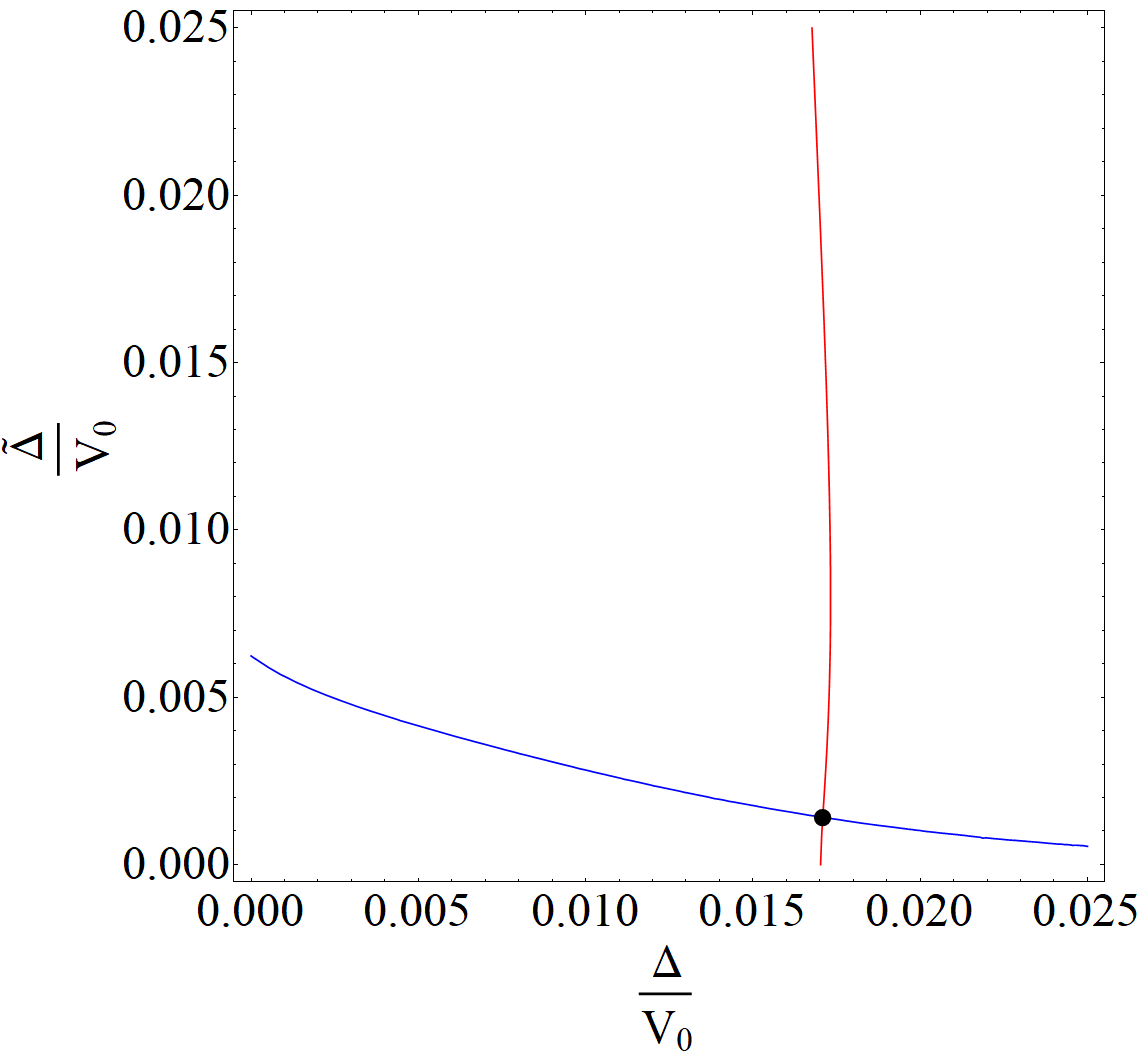
, and in the pairing part, where . The self-consistent solution is numerically obtained using Mathematica with error estimation to . Obviously this
represents a weak coupling case in which the kinetic part dominates.
Fig. 4 illustrates solutions of Eqs. (98) and (99) with the corresponding self-consistent solution.
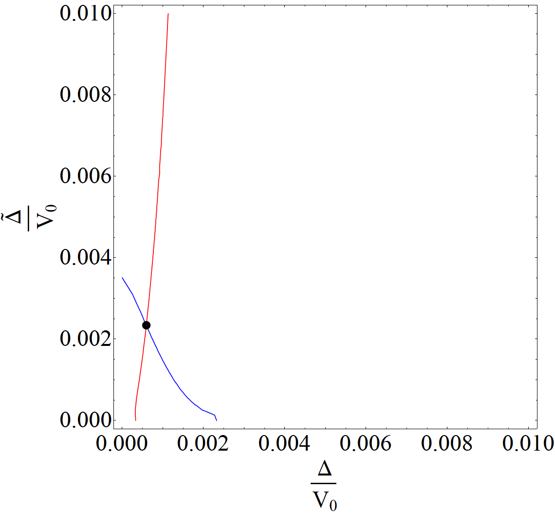
In the sLL, we found that Eqs. (98) and (99) do not support a coexistence of (non-zero) kinetic and pairing amplitudes, and thus, if only pairing is present it leads to a gapless (critical) -wave state at this level of approximation. We considered the question of coexistence when a cubic term is generated in the expansion (VI), in the kinetic part. The resulting equations are slightly modified Eqs. (98) and (99) (, etc.), and lead to a solution that describes a coexistence of pairing, where , and now where . The numerically obtained solution using Mathematica is shown in Fig. 5. The error is estimated to . Thus, this is a strong coupling, weak pairing case that can be identified with the usual Pfaffian-state case in which all composite fermions are paired in the same way of a -wave.
XI Conclusions
To conclude, we presented a microscopic derivation of the Dirac CF theory and proposed an effective (long-wavelength) noncommutative field-theoretical description. The developed formalism can serve as a base for a deeper understanding of the strongly correlated physics of the half-filled LL. The microscopic formulation is used to describe (in a mean-field approach) pairing instabilities of the half-filled LL. The description is consistent with the known experimental and numerical phenomenology and provides further insights into the nature of pairing instabilities.
References
- (1) B. I. Halperin, P. A. Lee, and N. Read, Phys. Rev. B 47, 7312 (1993).
- (2) G. Moore and N. Read, Nucl. Phys. B 360, 362 (1991).
- (3) D. T. Son, Phys. Rev. X 5, 031027 (2015).
- (4) V. Pasquier and F. D. M. Haldane, Nucl. Phys. B 516, 719 (1998).
- (5) N. Read, Phys. Rev. B 58, 16262 (1998).
- (6) Z. Dong and T. Senthil, Phys. Rev. B 102, 205126 (2020).
- (7) N. Read and D. Green, Phys. Rev. B 61, 10267 (2000).
- (8) G. Murthy and R. Shankar, Rev. Mod. Phys. 75, 1101 (2003).
- (9) A. C. Balram, M. Barkeshli, and M. S. Rudner, Phys. Rev. B 98, 035127 (2018).
- (10) R. V. Mishmash, D. F. Mross, J. Alicea, and O. I. Motrunich, Phys. Rev. B 98, 081107(R) (2018).
- (11) M. Yutushui and D.F. Mross, Phys. Rev. B 102, 195153 (2020).
- (12) L. Antonić, J. Vučičević and M. V. Milovanović, Phys. Rev. B 98, 115107 (2018).
- (13) N. Read, Phys. Rev. Lett. 62, 86 (1989).
- (14) M. V. Milovanović, S. Djurdjević, J. Vučičević and L. Antonić, Mod. Phys. Lett. B 34, 2030004 (2020).
- (15) A. C. Potter, M. Serbyn and A. Vishwanath, Phys. Rev. X 6, 031026 (2016).
- (16) C. Wang, N. R. Cooper, B. I. Halperin and A. Stern, Phys. Rev. X 7, 031029 (2017).
- (17) N. Seiberg, T. Senthil, C. Wang, E. Witten, Ann. Phys. 374, 395 (2016).
- (18) K. Prabhu, M. M. Roberts, arXiv: 1709.02814.
- (19) D. Karabali, V. P. Nair, A. P. Polychronakos, Nucl. Phys. B627, 565 (2002).
- (20) R. J. Szabo, Physics Reports, 378(4), 207-299 (2003).
- (21) N. Seiberg and E. Witten, JHEP 09, 032 (1999).
- (22) P. Aschieri, L. Castellani and M. Dimitrijević, Phys. Rev. D 87, 024017 (2013).
- (23) P. Aschieri, M. Dimitrijević, P. Kulish, F. Lizzi, & J. Wess. Noncommutative spacetimes: symmetries in noncommutative geometry and field theory (Vol. 774). Springer Science & Business Media, (2009).
- (24) B. Jurčo, S. Schraml, P. Schupp and J. Wess, Eur. Phys. J. C 17, 521 (2000).
Appendix A Basic structure of noncommutative gauge field theory
Noncommutative (NC) spaces are geometric structures for which the notion of a point loses its meaning. They arise naturally in physics, the most famous example being the “quantum” phase space of generalized coordinates and momenta, understood as mutually non-commuting (incompatible) observables that satisfy Heisenberg’s uncertainty relations . Another important example of NC space is realized by a single particle moving in the LLL; the guiding center coordinates of such a particle satisfy the following non-trivial commutation relation, . Finally, in the context of quantum gravity, the idea of NC geometry is applied to the structure of space-time itself. In this case, the degree to which space-time coordinates fail to commute is usually taken to be proportional to the square of the Planck length. For a more comprehensive review see, for example, Szabo.
Here we give a short review of the basic structure of a noncommutative gauge field theory based on the Seiberg-Witten (SW) construction, first presented in the context of String Theory SW_map1. An NC field theory is a field theory defined on a noncommutative space-time, i.e., a space-time described by mutually non-commuting coordinates, . One way to implement this NC structure is to deform the algebra of functions (fields) on ordinary (commutative) space-time, by introducing an NC star-product, the simplest of which is the Moyal-Weyl star-product,
| (102) |
The deformation parameters make a constant anti-symmetric matrix (hence the term constant noncommutativity). Note that the first term in the expansion (in powers of ) is just the ordinary commutative product of functions; higher order terms represent NC corrections. When applied to coordinate functions themselves, the above formula gives us
| (103) |
which is the simplest form of noncommutativity. Other types of noncommutativity are related to different star-products, (see ACD), but we will be working only with the Moyal-Weyl star-product. A more comprehensive account on various aspects of NC geometry and NC gauge field theory can be found in NCbook.
Let be a set of generators of a gauge group . Infinitesimal SW gauge variation (NC gauge transformation) of an NC field transforming in the fundamental representation of the gauge group (e.g. a matter field) is defined by
| (104) |
where stands for an NC gauge parameter. This transformation rule is analogous to the familiar one in ordinary, commutative gauge field theory, except for the noncommutative Moyal-Weyl star-product.
There is a notorious problem concerning the closure axiom for SW gauge transformations. Namely, assuming that NC gauge parameter is Lie algebra valued, , the commutator of two SW transformations is given by
| (105) | ||||
Due to the appearance of anticommutator , infinitesimal SW transformations do not in general close in the Lie algebra of a gauge group. A way to surmount this difficulty is to assume that NC gauge parameter belongs to the universal enveloping algebra (UEA), which is always infinite dimensional (Enveloping). This, however, leads to an infinite tower of new degrees of freedom (new fields), which is not a preferable property. To see this, consider a SW variation of the covariant derivative
| (106) |
with (here we only consider “left” gauge field; the case of “right” gauge field is treated in a similar manner). This implies the following transformation rule for the NC gauge potential,
| (107) |
meaning that it is also an UEA-valued object, which leaves us with an infinite number of new fields in the theory (one for each basis element of UEA).
SW map resolves this issue by demanding that NC fields can be expressed in terms of the NC parameter , commutative gauge parameter , commutative gauge potential , and their derivatives,
| (108) | ||||
| (109) |
where the ellipses stand for higher derivatives. In this way, NC theory is defined by the corresponding commutative one. There are no new degrees of freedom, just new interaction terms in the NC action.
NC gauge transformations are now induced by the corresponding commutative ones,
| (110) | ||||
| (111) |
with .
From (105) and (108) follows a consistency condition for NC gauge parameter,
| (112) |
which can be solved perturbatively (this makes sense because the star-product is also defined perturbatively). To this end, we represent the NC gauge parameter as an expansion in powers of the NC parameter , with coefficients built out of fields from the commutative theory,
| (113) |
The first term in the expansion (zeroth order in ) is the commutative gauge parameter .
An NC gauge parameter, up to first order in , is given by
| (114) |
where is a constant antisymmetric matrix of deformation parameters. In our case, where and is defined by and . Note that we work in dimensions and that the definition of implies that noncommutativity is realized only between spatial coordinates; it does not involve the time coordinate. Generalization to an arbitrary number of dimensions is straightforward.
Using the expansion (114) and the transformation rule (104) we readily obtain
| (115) |
Also, from (107) follows the transformation law for the NC gauge field,
| (116) |
In connection to our model, with left (L) and right (R) NC gauge transformations acting on NC CF fields and , it is convenient to combine the two CFs into a two-component spinor,
| (117) |
Under an NC gauge transformation it changes as
| (118) |
where . The NC gauge parameters have a special form given by
| (119) |
Infinitesimally, we get
| (120) |
Covariant derivative of is defined by
| (121) |
where we introduced left, , and right, , NC gauge potential. One can show that transforms covariantly,
| (122) |
provided that NC gauge potentials and transform in the following way:
| (123) |
The NC action (in Euclidean signature) reads as
| (124) |
where we have
| (125) |
In terms of components, the action is
| (126) | ||||
The SW map allows us to represent NC fields in terms of ordinary fields from the corresponding commutative theory; these commutative fields will be denoted by a hat symbol. NC fields are organized as perturbation series in powers of the deformation parameter, and they reduce to ordinary fields in the limit.
SW expansions of NC gauge parameters (up to first order) are (note the sign difference) given by
| (127) |
Likewise, SW expansions of L and R NC gauge potentials are (again, note the sign difference)
| (128) | ||||
| (129) |
with (commutative) gauge field strengths
| (130) |
Finally, the SW expansion of the NC matter field reads as
| (131) |
In particular, if we take and (both act as scalars), we get covariant derivatives (78) and (79), and the previous equation becomes
| (132) |
In general, to compute a first order NC correction for a product of two NC fields, we apply the following formula,
| (133) |
where and are first order NC corrections of and , respectively.
Thus, we can readily compute the NC covariant derivative,
| (134) |
with commutative field strengths and . Commutative covariant derivative is simply .
Appendix B The structure of NC covariant derivatives
Let us assume that the structure of NC covariant derivatives is given by Eqs. (76) and (77), i.e.,
| (137) | ||||
| (138) |
as consistent with the microscopic constraints.
If we want both (137) and (138) to transform covariantly, i.e.,
| (139) | ||||
| (140) |
we get two separate transformation laws for the gauge field (in the -case it acts from the right and in the -case from the left):
| (141) | ||||
| (142) |
Consistency of the two demands the following constraints:
| (143) | ||||
| (144) |
The second equation implies that , which is not consistent with being unitary. Thus, we must change the structure of the derivatives.
Now consider the case when two covariant derivatives have the same structure,
| (145) | ||||
| (146) |
with two gauge fields: the external background field (which is L gauge field for both fields and ) and (which is R gauge field for both fields and ). They transform under gauge transformations in the following way:
| (147) | ||||
| (148) |
In the commutative limit, these become simple gauge transformations,
| (149) | ||||
| (150) |
The relevant field represents an independent gauge field with respect to .
In the setup implied by (86) and (87), i.e.,
| (151) | ||||
| (152) |
we have to consider four different gauge fields and . Their transformation laws are given by
| (153) | ||||
| (154) | ||||
| (155) | ||||
| (156) |
However, these four fields are not mutually independent, , because aside from the external field, the theory can have only two more independent gauge fields, connected with two kinds of constraints. If we require that the difference of gauge fields transforms as a gauge field, we will have and , i.e., possibilities for independent gauge transformations, independent gauge fields, will be reduced to just one, but this would contradict our beginning set-up. That is why we need to take , and have two independent gauge transformations and fields and , in the commutative limit.