Sharp and fast bounds for the Celis-Dennis-Tapia problem
Abstract
In the Celis-Dennis-Tapia (CDT) problem a quadratic function is minimized over a region defined by two strictly convex quadratic constraints. In this paper we re-derive a necessary and sufficient optimality condition for the exactness of the dual Lagrangian bound (equivalent to the Shor relaxation bound in this case). Starting from such condition, we propose to strengthen the dual Lagrangian bound by adding one or two linear cuts to the Lagrangian relaxation. Such cuts are obtained from supporting hyperplanes of one of the two constraints. Thus, they are redundant for the original problem but they are not for the Lagrangian relaxation. The computational experiments show that the new bounds are effective and require limited computing times. In particular, one of the proposed bounds is able to solve all but one of the 212 hard instances of the CDT problem presented in [11].
keywords
CDT problem, Dual Lagrangian Bound, Linear Cuts.AMS
90C20, 90C22, 90C261 Introduction
The Celis-Dennis-Tapia problem (CDT problem in what follows) is defined as follows:
| (1) |
where , , , while is assumed to be positive definite. We will denote by
the ellipsoid defined by the second constraint, by its border, and by its interior.
The CDT problem was originally proposed in [12] and has
attracted a lot of attention in the last two decades. For some special cases a convex reformulation is available. For instance, in [24] it is shown that a semidefinite reformulation is possible when no linear terms are present, i.e., when . However, up to now no tractable convex reformulation of general CDT problems has been proposed in the literature. In spite of that, recently three different works [8, 13, 20] independently proved that
the CDT problem is solvable in polynomial time. More precisely, in [13, 20] polynomial solvability is proved by identifying all KKT points through the solution of a bivariate
polynomial system with polynomials of degree at most . The two unknowns are the Lagrange multipliers of the two quadratic constraints.
Instead, in [8] an approach based on the solution of a sequence of feasibility problems for systems of quadratic inequalities is proposed. The systems are solved
by a polynomial-time algorithm based on Barvinok’s construction [5].
Though polynomial, all these approaches are computationally demanding since the degree of the polynomial is quite large.
Conditions guaranteeing that the classical Shor SDP relaxation or, equivalently in this case, the dual Lagrangian bound is exact, are discussed in [2, 6]. In particular, in [2] a necessary and sufficient condition is presented. It is shown that lack of exactness is related to the existence of KKT points with the same Lagrange multipliers but two distinct
primal solutions, both active at one of the two constraints but one violating and the other one fulfilling the other constraint.
In [9] necessary and sufficient conditions for local and global optimality are discussed based on copositivity.
In [10] an exactness condition is given for a copositive relaxation, also for the case with additional linear constraints.
A trajectory following method to solve the CDT problem has been discussed in [24], while different branch-and-bound solvers are tested in [17].
Recently, different papers proposed valid bounds for the CDT problem.
In [11] the Shor relaxation bound is strengthened by adding all RLT constraints obtained by supporting hyperplanes of the two ellipsoids. By fixing the supporting hyperplane for one ellipsoid, the RLT constraints obtained with all the supporting hyperplanes of the other can be condensed into a single SOC-RLT constraint. Varying the supporting hyperplane of the first ellipsoid gives rise to an infinite number of SOC-RLT constraints which, however, can be separated in polynomial time. The addition of these constraints does not allow to close the duality gap but it is computationally shown that many instances which are not solved via the SDP bound, are solved with the addition of these SOC-RLT cuts. The authors generate 1000 random test instances for each ,
following a procedure described in [16] to generate trust-region problems with one local and nonglobal minimizer. The proposed bound based on SOC-RLT cuts allows to solve most instances except for 212 (38 for , 70 for , and 104 for ). Such unsolved instances are considered as hard ones in subsequent works.
In [23] lifted-RLT cuts are introduced and it is shown that the new constraints allow to derive an exact bound for but also to improve the bounds of [11] over the hard instances for .
In [25] it is proved that the duality gap can be reduced to 0 by solving two subproblems with SOC constraints when the second constraint is the product of two linear functions.
In [3] KSOC cuts are introduced. These are Kronecker product constraints which generalize both the classical RLT constraints obtained from two linear inequality constraints, and the SOC-RLT constraints obtained
from one linear inequality constraint and a SOC constraint. Further hard instances from [11] are solved with the addition of these cuts.
In this paper we investigate ways to strengthen the dual Lagrangian bound through the addition of one or two linear cuts. In particular,
the paper is structured as follows.
In Section 2 we derive some theoretical results for a class of problems with two constraints which includes the CDT problem as a special case.
We develop a bisection technique to solve the dual Lagrangian relaxation for such class of problems.
In the following sections we apply the results of Section 2 to the CDT problem.
In particular, in Section 3 we introduce some results through which it will be possible to re-derive the necessary and sufficient exactness condition discussed in [2].
In Section 4 we discuss how to improve the dual bound for the CDT problem by the addition of a linear cut. Next, in Sections 5-6 we discuss techniques to further improve the bound. More precisely, in Section 5 we still present a bound based on the addition of a linear cut but we develop a technique to locally adjust a given linear cut, while in Section 6 we consider a bound based on the addition of two linear cuts.
Finally, in Section 7 we present some computational experiments which show that the newly proposed bounds, in particular those based on two linear cuts, are both computationally cheap and effective. In particular, one of the bounds will be able
to solve all but one of the hard instances from [11]. We also investigate which are the most challenging instances for the proposed bounds and, as we will see, the difficulties are related to the existence of multiple solutions
of Lagrangian relaxations.
2 Lower bounds obtained from the Lagrangian relaxation
The CDT problem (1) is a specific instance of the following, more general, one:
| (2) |
In this section, we discuss a class of lower bounds on the solution of problem (2) that can be obtained from its Lagrangian relaxation. In the next sections, we will apply these bounds to the specific case of the CDT problem (1). Throughout this and the following sections, we make the following assumptions.
Assumption 2.1.
Note that if the last condition in Assumption 2.1 is violated, we can find the solution of Problem (2) by removing the last constraint and the relaxation discussed in this section is useless. Now, let and . Let be a closed subset of and for , with , define the Lagrangian relaxation
| (4) |
and the corresponding solution set
Note that is compact, since is nonempty (in view of part c) of Assumption 2.1) and compact (in view of the compactness of which follows from parts a) and b) of Assumption 2.1), and is continuous. Due to well-known properties of the Lagrangian relaxation, we have that function is such that , and is concave (it is the pointwise minimum of a set of functions linear in ). The best bound that can be obtained as the solution of (4) is given by
| (5) |
and corresponds to the solution of the dual Lagrangian problem. Note that function depends on the choice of set .
Now, we recall that the supergradient of a function at , is defined as
Since is concave, for any , the supergradient is non-empty.
For define the following subset of
For , define a (set-valued) function
| (6) |
( denotes the set of nonnegative reals and is the power set of the set of real numbers). Also set , . The following proposition shows that function is monotone non-increasing (see Definition 3.5.1 of [4]) and upper semicontinuous (see Definition 1.4.1 of [4]). These two properties will play an important role in the computation of a lower bound for Problem (2). Moreover, this proposition characterizes the supergradient of at each .
Proposition 1.
For any
i) is monotone not-increasing, that is if , , , then .
ii) is upper semicontinuous, that is, if , where is an open subset of , then there exists a neighborhood of such that .
iii) .
Proof.
i) Let be such that and , then and . By adding up the previous inequalities, it follows that , which implies the thesis.
ii) It is a consequence of Berge’s Maximum Theorem (see [7]). In particular, we consider the slightly different formulation presented as the corollary to Theorem 3 on page 30 of [14]. Namely, since function , is continuous, set valued function is upper semicontinuous. Hence, also is upper semicontinuous, since it is obtained as the composition of with , which is continuous (see Theorem 1’ on page 113 of [7]).
iii) It is a consequence of Theorem 4.4.2 in [15], being compact.
The next proposition characterizes the optimal solution of the dual Lagrangian problem (5).
Proposition 2.
Proof.
We first prove that the value is attained. Let be an optimal solution of problem (3). Since (more precisely, it belongs to the interior of ) and recalling that , it holds that . Then, for each
(recall that in view of part c) of Assumption 2.1). Thus, the maximum value of is attained at some . But in view of part d) of Assumption 2.1, we have that . Thus, function is increasing at and, consequently, we must have . Moreover, by the optimality condition of nondifferentiable concave functions, must hold.
The following property shows that it is always possible to find a sufficiently high value of such that , that is, the elements of are feasible solutions of Problem (2).
Lemma 3.
Proof.
By contradiction, assume that there exists such that and let be such that , then . Since , it follows that which contradicts the assumption on .
The following proposition shows that if , then is equal to the optimal value of Problem (2).
Proposition 4.
Under Assumption 2.1 the following statements are equivalent:
i) ,
ii) and there exists such that .
Proof.
i) ii). Let be such that and . Let be a solution of (2). Then, , hence . Moreover, .
ii) i). Assume that and let . Then, by ii), . It follows that and .
Remark 5.
If , by point iii) of Proposition 1, , so that corresponds to a maximizer of the dual Lagrangian. Note that equation always admits a solution if is continuous. However, in the general case, is only upper semicontinuous. In this case, the value of for which may not satisfy . Thus, the optimal value of the dual Lagrangian (5) is not equal to the optimal value of (2) but it represents a lower bound of it.
In order to evaluate a numerical solution algorithm, we define the following weak solution of (2).
Definition 6.
is an -solution of (2) if and .
The following proposition presents a bound on the error committed on the estimation of .
Proposition 7.
For any such that , and for any , it holds that , i.e., is an -solution of problem of (2) with .
Proof.
Since and observing that for any , , from which .
Now we introduce Algorithm 1 which is based on a binary search through different values and is able to return the solution of the dual Lagrangian problem, i.e., the maximum of function and, in some cases, even the solution of problem (2). The algorithm also returns a point and (possibly) a point . Note that according to Proposition 7, point is an -solution of problem of (2) with .
DualLagrangian(, )
The algorithm starts with an initial interval of values , where is a suitably large value and can be set equal to as defined in Lemma 3. At each iteration the algorithm halves such interval by evaluating the set at . Then, the algorithm sets: , if ; if . Instead, if , the algorithm sets and exits the loop.
The following proposition characterizes Algorithm 1.
Proposition 8.
i) Algorithm 1 terminates in a finite number of iterations,
ii) at each iteration ,
iii) at termination ,
iv) at each iteration, if , then ,
v) point is an -solution of (2) with .
Proof.
i) At each iteration the length of the interval is halved. Hence, in a sufficient large number of iterations, the termination condition of the main loop will be satisfied.
ii) At the beginning of the algorithm we have that . Every time is updated, we set if condition holds. Since , by the monotonicity of function , which is a consequence of the monotonicity of function , condition is maintained. The same reasoning can be used to prove that .
iii) It is a consequence of ii) and the termination condition.
iv) , due to point ii) and the monotonicity of functions and , which is a consequence of the monotonicity of function .
v) It is a consequence of Proposition 7.
The following property is a direct consequence of the upper semicontinuity of .
Proposition 9.
Let be such that , then there exists a neighborhood of such that .
As a consequence of the previous proposition, it is possible to improve the lower bound on Problem (2), obtained as the solution of (4), by replacing set with a different set fulfilling a given condition.
Proposition 10.
Let be such that or, equivalently, , and assume that . Then .
Proof.
If , then and by Proposition 4 . Thus, we only consider the case . In such case, by Proposition 9, . Since , there exists such that . Note that . If , then, by Proposition 4, , so that the thesis is satisfied in view of . Otherwise, if , let be such that . Then , where we used the facts that and that .
The following proposition deals with the special case of the previous result when .
Proposition 11.
Let be such that , and assume that . Then .
Proof.
Since we have that and, consequently, since , also . Then, implies . Moreover, if , then the condition is satisfied and the result follows from Proposition 10.
Stated in another way, the previous propositions show that, in case the lower bound is not exact, we are able to improve (increase) it, if we are able to replace set with a new set which cuts away all members of outside .
Remark 12.
Up to now we have not discussed the difficulty of computing the values of function or, equivalently, the difficulty of solving problem (4). Such difficulty is strictly related to the specific problem (i.e., to the specific functions ), and also to the specific set . In the next sections we apply the general theory developed in this section to the CDT problem. We show that for suitably defined sets (defined by one or two linear cuts), the computation of function can be done in an efficient way, and, moreover, the corresponding lower bounds improve the standard dual Lagrangian bound, corresponding to the case .
Remark 13.
In principle one could also define a cutting algorithm where a sequence of sets is generated such that: i) for all ; ii) ; iii) . The corresponding sequence of lower bounds is strictly increasing in view of Proposition 11, and converges to . However, the difficulty related to such an algorithm is that forcing ii) may not be trivial and, moreover, as already commented in Remark 12, computing may be computationally demanding.
The following Algorithm 2, in principle, is able to always find an approximate solution of (2). The algorithm is based on an iterative reduction of set , in order to eliminate its elements in which function is positive. In practice, Algorithm 2 could be unimplementable. Indeed, it may require a large number of cuts on set and each added cut may increase the complexity of the optimization problem that we need to solve to evaluate DualLagrangian. In Section 5, we will see that, to refine the lower bound on the solution of the CDT problem, it is computationally more convenient to adjust existing cuts instead of adding new ones. We stress that we will not actually use Algorithm 2 for the solution of the CDT problem. We present this algorithm just as a theoretical contribution.
Proposition 14.
Algorithm 2 terminates and is such that and .
Proof.
By contradiction, assume that the algorithm does not terminate. Let be the value of returned by the -th call to DualLagrangian. Sequence is monotone non increasing, moreover the domain of the sequence is a subset of finite cardinality of interval (its maximum cardinality depends on and ). Indeed, the termination condition of function DualLagrangian allows only for a finite number of divisions of the interval . Hence, sequence converges in a finite number of iterations to its limit and there exists such that . By iv) of Proposition 8, and, since the algorithm does not terminate, . At the -iteration, the algorithm calls , which returns the value . Anyway, at the previous iteration , the elements at which function is positive had already been removed from . This implies that cannot return the strictly positive value , leading to a contradiction. Hence, the algorithm terminates and the stated bounds hold because of the termination condition and by Proposition 7.
3 Lagrangian relaxation of the CDT problem
In this section, we apply the general properties presented in Section 2 to the CDT problem (1). In fact, the CDT problem is a specific instance of (2) in which , , .
Note that the first two requirements of Assumption 2.1 are satisfied; in order to satisfy the third one we assume that
| (8) |
i.e., the feasible region of (1) has a nonempty interior. Note that the assumption can be checked in polynomial time by the solution of a trust region problem. As before, we denote by a closed set such that , i.e., it contains the ellipsoid defined by the second constraint. For each , the Lagrangian relaxation (4) takes on the form
| (9) |
If , this is the standard Lagrangian relaxation of problem (1) and it can be solved efficiently since it is a trust region problem. Following the notation of Section 2, let
be the set of optimal solutions of (9). To apply Algorithm 1 to the CDT problem with , we need to characterize the set of optimal solutions of problem (9) with , which is a trust region problem. The set of optimal solutions of a trust region problem has been derived, e.g., in [1, 18, 19]. Here we briefly recall the different cases. For simplicity, let and . We distinguish the following cases:
- Case 1
-
If and, then is the unique optimal solution of (9);
- Case 2
-
Let be the orthonormal eigenvectors of matrix , and let be the corresponding eigenvalues. Let and . For each such that , let
where
Then, we have the following subcases:
- Case 2.1
-
It holds that for some . Then, there exists a unique such that and is the unique optimal solution of (9);
- Case 2.2
-
It holds that for all but . In this case there exists a unique such that and is the unique optimal solution of (9);
- Case 2.3
-
It holds that for all and . In this case we have that is not a singleton and is made up by the following points:
(10) Thus, we recognize two further subcases:
- Case 2.3.1
-
, in which case contains exactly two distinct points;
- Case 2.3.2
-
, in which case the set contains an infinite number of points and is a connected set.
Note that in Cases 2.3.1 and 2.3.2 we can compute the two values by solving a trust region problem over the border of a -dimensional ball. More precisely, we need to solve the following problems:
| (11) |
where . In these cases, where is not a singleton, we also set
| (12) |
while in all other cases, when is a singleton, we set
| (13) |
The following statement is a direct consequence of
Proposition 4.
Proposition 15.
Proof.
Since , in the first two cases and the thesis is a consequence of Proposition 4. If and , we observed that is a connected set. Then, there exists such that . More precisely, is a point along the curve in connecting points and , defined in (12). Thus, the lower bound is equal to the optimal value of problem (1).
Note that the first two conditions of Proposition 15 imply exactness of the bound also for generic regions , while the last condition is specific to the case . The following result is related to the necessary and sufficient condition under which the dual Lagrangian bound is not exact discussed in [2].
Proposition 16.
In the CDT problem (1), if and only if contains exactly two points, i.e., (Subcase 2.3.1), and .
Proof.
It is a consequence of Proposition 15 and the fact that for it holds that .
Now, we introduce an example where , that is the dual Lagrangian bound is not exact, which will also be helpful in the following sections.
Example 17.
Let us consider the following example taken from [11]:
Such instance has optimal value attained at points and . The maximizer of is for which we have:
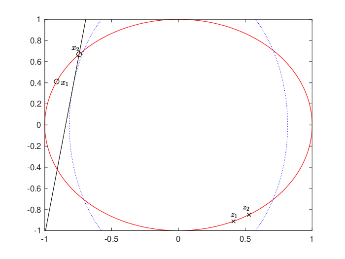
and, moreover, , so that we have exactly two optimal solutions of (9), one violating the second constraint, namely , point in Figure 1, displayed as , the other in , point in Figure 1, displayed as . The lower bound is , which is not exact.

In the next sections we will try to improve the dual Lagrangian bound (or the equivalent SDP bound) by adding linear cuts, i.e., by introducing regions defined by one or two linear cuts.
4 Bound improvement
We assume that the dual Lagrangian relaxation is not exact, i.e., as previously stated in Proposition 16
Recall that, by Proposition 16, in this case, there exists a single point (actually ), and a single point .
Now we show that the dual Lagrangian bound can be strictly improved through the addition of a linear cut.
We first observe that the optimal value of problem (1) does not change if we
add constraints which are implied by the second one.
In the following proposition, we define a projection , that
maps to the element of located
on the segment that joins to the center of the ellipsoid (given by ).
Proposition 18.
For , set , where is the center of the ellipsoid. Then .
Proof.
Note that (it is a consequence of the fact that function is quadratic and it can be verified by direct substitution). Then .
Given any , it holds, by convexity, that
Thus, the following linear constraint is implied by the second constraint in (1):
| (14) |
and, consequently, it can be added to problem (1) without modifying its feasible region. In particular, if , being , the linear constraint is
Due to the redundancy of the lienar constraint for problem (1), we can define, for a given , the new Lagrangian problem
| (15) |
where
| (16) |
If we set , i.e., is the projection over of the single point in , then and, moreover, , so that, by Proposition 11, . Then, if we run again Algorithm 1 with input defined in (16) and (or ), we are able to improve strictly the dual Lagrangian bound. Note that problem (15), needed to compute function , can be solved in polynomial time according to the results proved in [11, 21]. But we also discuss an alternative way to solve problem (15), based on the solution of a trust region problem. For , after the addition of the linear cut, a unique optimal solution exists, lying in and, consequently, in , since also the linear constraint in (15) is not active at it, being a subset of the region defined by the linear cut. By continuity, for values smaller than but close to , the unique optimal solution of (15) also lies in , i.e., with . Thus, such optimal solution must be a local and nonglobal optimal solution of the trust region problem (9) with . Indeed, the globally optimal solution of this trust region problem always violates the second constraint in (1) for all . Now, for a generic , we first check whether a local and nonglobal optimal solution of problem (9) with exists, by exploiting the necessary and sufficient condition stated in [22]. Also recall that, if it exists, the local and nonglobal minimizer is unique. If it does not exist, then the linear constraint must be active at all optimal solutions of problem (15). In this case we set . Otherwise, if it exists, we denote it by . If , then we set again , otherwise we denote by the value of the objective function of (15) evaluated at . Then, we consider the best feasible solutions of problem (15) for which the linear constraint is imposed to be active. The resulting problem is converted into a trust region problem, after the change of variable , where is a matrix whose columns form a basis for the null space of vector . The resulting (trust region) problem is:
| (17) |
where is constant with respect to the vector of variables . Let be the set of optimal solutions of problem (17) and
Note that the set can be computed through the procedure presented in Section 3 with the different cases (namely, Cases 1, 2.1, 2.2, 2.3.1, 2.3.2) after rewriting it as a classical trust region problem. Moreover, let be the optimal value of problem (17). Now, after comparing and , we are able to define the set of optimal solutions for problem (15). More precisely, if , then , i.e., is the unique optimal solution of problem (15). In this case
Instead, if , which always holds, e.g., if , then . Since all points in lie over a supporting hyperplane of , we must have that
and equality holds only if . In the latter case, the bound is exact, otherwise Algorithm 1 sets . Finally, if , then and in this case and the algorithms exits the loop. The following result is a straightforward consequence Proposition 11.
Proposition 19.
Algorithm 1 with will stop after a finite number of iterations or will converge to some with a new lower bound .
Proof.
Strict inequalities hold in view of Proposition 11 with and , since, as already observed, .
If the final bound is not exact, i.e., , at we have and contains multiple optimal solutions, in particular, one in and the other(s) outside . We illustrate all this on Example 17.
Example 20.
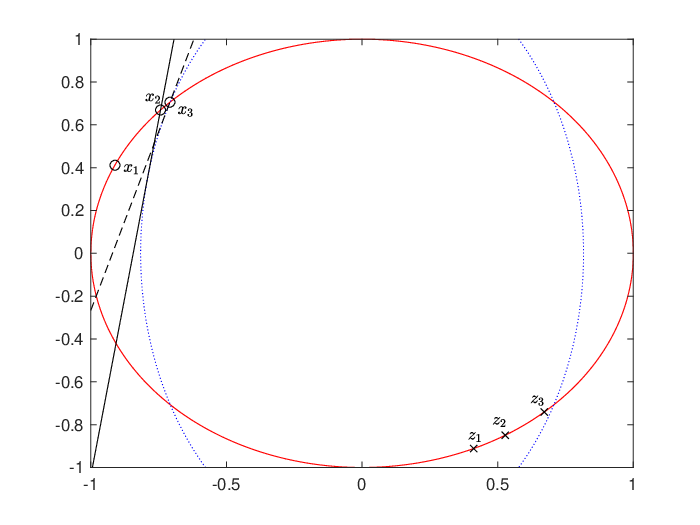
The optimal solution of (9) with for which violates the second constraint is . The lower bound is . After the addition of the linear inequality (14) obtained with , equal to the projection of over the boundary of the second constraint, we can run again Algorithm 1 with and we get to and , which improves the previous lower bound. In Figure 2 we show the linear cut and the two new optimal solutions outside and in ( and , respectively) obtained at . In the same figure we also display the previous pair of optimal solutions in order to show the progress of the algorithm.
5 Improving the bound by local adjustments of the linear cut
In the previous section we proposed to set equal to the projection over of , the optimal solution of problem (9) with lying outside . However, this point can be improved by some local adjustment. To this end, we should search for some perturbation direction such that
for all . Taking into account that the linear cut in (15) is active at , the above inequality is equivalent to
| (18) |
If such direction exists, then we are able to improve the linear cut by replacing with
| (19) |
for some and small enough. By (18), for any positive step along direction we have and, by continuity, that holds true also in a small neighborhood of . However, if we take too large a step along direction , then new optimal solutions of problem (15) with replaced by , sufficiently far from , may appear. But if we take a small enough step along direction , then no new optimal solution will appear and the only optimal solution of problem (15) with replaced by will be point . Thus, as a consequence of Proposition 10, Algorithm 1 with input will be able to further reduce the value and improve (increase) the lower bound. Therefore, the question now is how to find a direction fulfilling (18) or to establish it does not exist. We discuss different cases depending on the cardinality of (see the cases discussed in Section 3 for the trust region problem).
5.1
In this case, let be the unique point in , then we need to solve the following convex optimization problem
whose optimal solution is and its optimal value is . Therefore, if we are always able to locally adjust the current point in such a way that the bound can be improved.
5.2
In this case, let and be the two optimal points in . Then, we need to solve the following optimization problem
| (20) |
or, equivalently
This is a convex optimization problem, whose solution can be obtained in closed form. Indeed, by imposing the KKT conditions, it can be seen that the optimal solution has the following form
| (21) |
Now, let
By replacing (21) in the objective function of (20), we have that (20) can be rewritten as
The optimal solution of this problem is
Then, the optimal value is:
We notice that ,
and, by Cauchy-Schwarz inequality:
and equality holds if and only if and are linearly dependent. Thus, the optimal value of (20) is always strictly positive unless the two vectors and lie along the same direction. More precisely, the optimal value is null only if the two vectors have the same direction but opposite sign. Indeed, let
Then, we have and . If is positive, then either (if ), or (if ) occurs, so that the optimal value is equal to or and is, thus, positive. If is not a negative multiple of , we are able to locally adjust along direction
5.3 is an infinite connected set
In this case we need to solve the following optimization problem
| (22) |
An improving direction exists if and only if the optimal value of this problem is strictly positive (note that the optimal value is always nonnegative since the inner minimization problem has optimal value 0 for ). We first remark that the problem is convex. Indeed, for each fixed , we have a concave function with respect to , and the minimum of an infinite set of concave functions is itself a concave function (to be maximized, so that the problem is convex). The inner minimization problem can be solved in closed form. After removing the terms which do not depend on , the inner problem to be solved is
According to Subcase 2.3.2 in Section 3, can be written as in (10) and the minimization problem can be reduced to the computation of the minimum of a linear function over the unit sphere:
where is some linear function of and is the multiplicity of the minimum eigenvalue of the matrix , corresponding to the Hessian of the objective function of problem (17). The optimal solution of this problem is
while the optimal value is .
5.4 An algorithm for the refinement of the bound
Let and be defined as in Section 4. We propose Algorithm 3 for a bound based on successive local adjustments of the linear cut. In line 2, Algorithm 1 is run with input and . Note that with a slight abuse here we are assuming that the algorithm returns and the related points and , while in practice close approximations of these quantities are returned, namely , and . In line 3, is initialized with the input point itself and the direction , following the discussion in Section 5.1, is set equal to the difference between , the point outside returned by Algorithm 1, and . The outer while loop of the algorithm (lines 4-20) is repeated until the bound is improved by at least a tolerance value . Inside this loop, in line 5 the initial step size is set and a new incumbent is computed. The inner while loop (lines 7-15) computes the step size: until the optimal value of problem (15) with and , denoted by , is lower than the current lower bound , we need to decrease the step size and recompute a new incumbent (lines 10-11). If the step size falls below a given tolerance value, we exit the inner loop and also the outer one. Otherwise, we have identified a new valid incumbent and we set to 1 the exit flag for the inner loop (line 13), so that, later on, a new linear inequality (14) with will be computed. Then, at line 17 we run Algorithm 1 with input and . Finally, in line 18, we update point and the direction . We remark that at each iteration is one optimal solution of the current subproblem (15) with lying outside and at which the linear cut of the subproblem is active, i.e., . As seen in Section 5.1, if , i.e., is the unique optimal solution of the current subproblem (15) with lying outside , then, in view of Proposition 10, the local adjustment employed in Algorithm 3 is guaranteed to improve the bound. However, as seen in Sections 5.2 and 5.3, if contains more than one point, than the proposed local adjustment is not guaranteed to improve the bound. Sections 5.2 and 5.3 suggest how to define perturbing directions which still allow to improve the bound, in case they exist. However, as we will see through the computational experiments, Algorithm 3 turns out to be time consuming and it is more convenient to improve the bound by adding a further linear cut, as we do in Section 6, rather than further locally adjusting the current linear cut. In order to clarify this point, we can make a comparison with Integer Linear Programming (ILP). In ILP problems, once a linear relaxation is solved, a valid cut removes one optimal solution of the relaxation. If the optimal solution is unique, then after the addition of the valid cut, the bound improves. But if the linear relaxation has got multiple solutions, then the valid cut is not guaranteed to remove all of them and, thus, the bound may not improve. It is possible to try to strengthen the valid cut in such a way that all optimal solutions of the linear relaxations are removed. But, more commonly, new linear cuts are added.
Input:
Now we apply Algorithm 3 to our example.
Example 21.
We have that is initialized with and with . During the execution of Algorithm 3, and are updated as indicated in Table 1.
| Iteration | ||
|---|---|---|
| 1 | ||
| 2 | ||
| 3 | ||
| 4 | ||
| 5 | ||
| 6 | ||
| 7 |
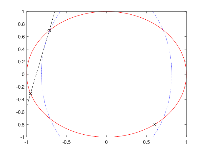
Interestingly, the best bound obtained in the example is exactly the one obtained for the same problem by the approach proposed in [11], based on the addition of SOC-RLT constraints. Figure 3 displays the situation at the last iteration of Algorithm 3. Problem (15) has got three optimal solutions, one in and two outside . The two optimal solutions outside are opposite to each other with respect to the final vector , so that, as discussed in Section 5.2, no further local adjustment is possible to improve the bound in this case.
6 Bound improvement through the addition of a further linear cut
Another possible way to improve the bound is by adding a further linear cut to (15). Let and be defined as in Section 4. In line 2 of Algorithm 3, we compute , and, later on, we try to locally adjust . Rather than doing that, we can add a further linear cut, cutting away. In particular, we add the one obtained through the projection over of . Let be such projection. Then, we define the following problem
| (23) |
which is equivalent to problem (9) where
A convex reformulation as the one proposed in [11, 21] for problem (15) is not available in this case (unless the two linear inequalities do not intersect in the interior of the unit ball). But in this case the alternative procedure discussed in Section 4 turns out to be useful. As before, for each value in the while loop of Algorithm 1 we can first check whether a local and nonglobal optimal solution of problem (9) with exists, by exploiting the necessary and sufficient condition stated in [22]. If it exists, and belongs to , we denote it by . Next, we need to compute the optimal value of (23) when at least one of the two linear constraints is active, i.e., we need to solve the following problem
| (24) |
A convex reformulation of this problem has been proposed in [24]. Alternatively, one can solve two distinct problems, each imposing that one of the two linear inequalities is active. Each of these problems can be converted into a trust region problem with an additional linear inequality, which can be solved in polynomial time through the already mentioned convex reformulation proposed in [11, 21]. Thus, we compute the set of optimal solutions of (23) for which the first linear cut is active, and then the set of optimal solutions of (23) for which the second linear cut is active. Finally, the optimal values of these problems are compared with the value of the local and nonglobal minimizer (if it exists) in order to identify the set of optimal solutions of (23). At this point we are able to compute and update and accordingly. If for some we have that and , i.e., problem (23) has an optimal solution in and (at least) one optimal solution outside , then and Algorithm 1 stops. We illustrate all this on Example 17.
Example 22.
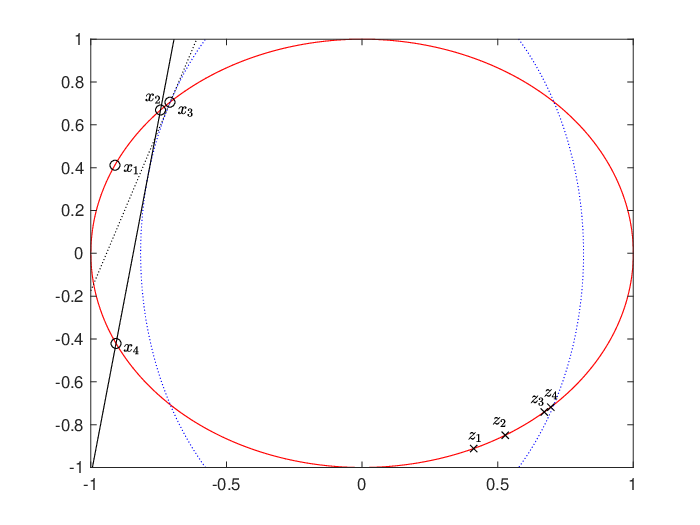
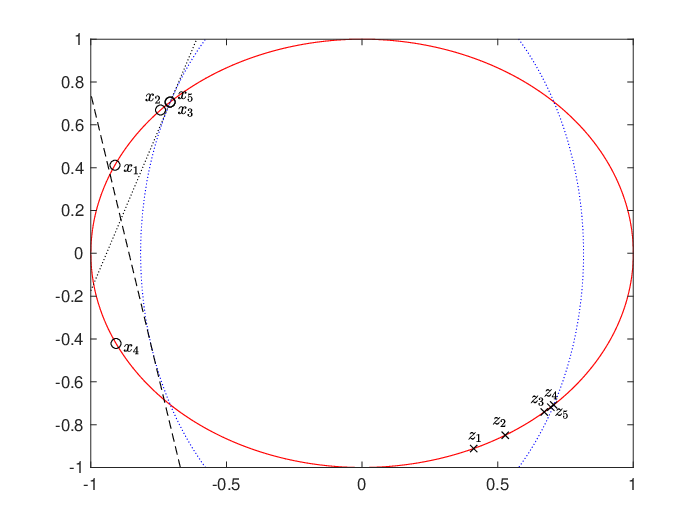
We add a second linear cut obtained through the projection over of the optimal solution of problem (15) with outside . This leads to a further improvement with and , which almost closes the gap. In Figure 4 we show the two linear cuts and the two new optimal solutions, one outside and one belonging to ( and , respectively). Again, we also report the previous pairs of optimal solutions in order to show the progress.
Now, assume that the returned bound is not exact. Also in this case and can be locally adjusted. One can combine the techniques presented in Section 5 and in the current section, by using a technique similar to the one described in the former section to improve the pair of points and . In particular, at we have one optimal solution of problem 23 belonging to , namely the local and nonglobal optimal solution of problem (9) with , and at least another one outside . We denote the latter by and we observe that at least one of the two linear cuts is active at this point, i.e., either or (or both). Then, if only the first cut is active at , we update as follows for a sufficiently small value, while . If only the second cut is active, we update as follows , for a sufficiently small value, while . Finally, if both are active we select one of the two cuts and perturb it. After the perturbation, we run again Algorithm 1 with input and , and we repeat this procedure until there is a significant reduction of the bound. Note, however, that it might happen that no improvement is possible. In case and (similar for and ), then the proposed perturbation for sufficiently small, allows to improve the bound. Indeed, in such cases the local adjustment is able to cut the unique solution outside away. In order to illustrate other different cases we employ Figures 5(a)-5(c). As usual, in these figures the point in is denoted by , while the others (outside ) are denoted by . If and , (see Figure 5(a)), or and (see Figure 5(b)), then it is not possible to remove all the solutions outside by perturbing a single linear cut. Indeed, in both cases the perturbation of a single linear cut is able to remove just one of the two optimal solutions outside . But it is possible to remove both by perturbing both linear cuts. Instead, Figure 5(c) illustrates a case where and . In this case even the perturbation of both linear cuts is unable to remove all three solutions outside . The only way to remove all three solutions outside is through the addition of a further linear cut, but, of course, this leads to a more complex problem with one trust region constraint and three linear inequalities.


Example 23.
In our example, this refinement is finally able to close the gap and return the exact optimal value . In Figure 6 we report the result of the first perturbation of the linear cuts. Since only the second linear cut is active at , in this case the second linear cut is slightly perturbed and becomes equivalent to the tangent to at the optimal solution of the original problem (1). It is interesting to note that the new optimal solution outside , indicated by , lies in a different region with respect to the previous ones and is further from with respect to and (the reduction of reduces the penalization of points outside ). Such solution is cut by the new linear inequality, obtained by a (not so small) perturbation of the first linear cut, displayed in Figure 7, together with the two new optimal solutions ( and ), now corresponding to the two optimal solutions of problem (1).
7 Computational Experiments
In this section we report the computational results for the proposed bounds over the set of hard instances selected from the random ones generated in [11] and inspired by [16].
More precisely, in [11] 1000 random instances were generated for each size . Some of these instances have been declared hard ones, namely those for which the bound obtained
by adding SOC-RLT constraints was not exact. In particular, these are 38 instances with , 70 instances with , and 104 instances with . Such instances have been made available in GAMS, AMPL, and COCOUNT formats
in [17]. We tested our bounds on such instances.
All tests have been performed on an Intel Core i7 running at 1.8 GHz with 16GB of RAM. All bounds have been coded in MATLAB.
We computed the following bounds:
- •
LbDual, the dual Lagrangian bound computed through Algorithm 1 with input ;
- •
LbOneCut, the bound obtained by adding a single linear cut and computed through Algorithm 1 with input ;
- •
LbOneAdj, the bound obtained by local adjustments of the added linear cut as indicated in Algorithm 3;
- •
LbTwoCut, the bound obtained by adding two linear cuts;
- •
LbTwoAdj the bound obtained by adjusting the two linear cuts.
According to what done in [3, 11, 23], an instance is considered to be solved when the
relative gap between the lower bound, say , and the upper bound, say , is not larger than , i.e.,
We set equal to the lowest value obtained by running, after the addition of the first linear cut, two local searches for the original problem (1), one from
the optimal solution of (15) returned at the end of Algorithm 1, and the other from an optimal solution of the same problem outside .
In Tables 2-4 we report the average and maximum relative gaps for each bound, and the average and maximum computing times for , respectively.
Moreover, the average computing time for bound LbTwoAdj is computed only over the instances (87 overall, as we will see) which are not solved by bound LbTwoCut, while
for bounds LbTwoCut and LbTwoAdj the average gap is taken over the instances which were not solved by these bounds.
We remark that the bound LbTwoCut is computed by adding the first cut as in bound LbOneCut, i.e., the supporting hyperplane at , and then adding a further linear cut through the projection of an optimal solution outside obtained when computing
bound LbOneCut, i.e., point returned by procedure with input . We could as well choose the adjusted cut computed by bound LbOneAdj as the first cut for bound LbTwoCut, but we observed that with this choice no improvement over LbOneAdj is obtained.
This is related to what already observed in Figure 3: bound LbOneAdj cannot be improved any more when there are (at least) two optimal solutions outside (besides the one in )). Thus, the second cut
is able to remove one of such optimal solutions but not the other, so that the bound cannot be improved.
Similarly, for bound LbTwoAdj the two initial cuts are the ones computed for bound LbTwoCut.
For what concerns the computing times, we observe that these are lower than those reported in [23] for the bound
obtained with the addition of SOC-RLT cuts (around 4s for an instance with ) and for the bound obtained by adding lifted-RLT cuts (around 92s for an instance with ).
They are also lower than those reported in [3] for the bound obtained by adding KSOC cuts (up to 2s for instances). For the sake of correctness, we point out that the computing times reported in those papers have been obtained with different processors. However, such processors have comparable performance with respect to the one employed for the computational experiments in this paper.
In general, the proposed bounds are very cheap. Only for two instances with , LbTwoAdj required times above 1s (around 1.5s in both cases). Usually the computing times are (largely) below 1s.
Both the dual Lagrangian bound and the bound obtained by a single linear cut are pretty cheap but with poorer performance in terms of relative gap. The bound obtained by Algorithm 3
with a local adjustment of the linear cut is better than the two previous ones in terms of gap but is also more expensive (although still cheap).
The bound LbTwoCut offers a good combination between quality and cheap computing time. But a more careful choice of the two linear cuts, through a local adjustment, improves the quality without compromising the computing times.
This is confirmed by the results reported for . Although this bound is more expensive than the others, the additional search for adjusted linear cuts further increases the quality of the bound.
In Table 5 we report the number of solved instances for LbTwoCut and LbTwoAdj.
According to what reported in [3], the total number of unsolved instances out of the 212 hard instances is equal to:
133 for the bound proposed in [23] (18 with , 49 with , and 66 with );
85 for the bound proposed in [3] (18 with , 22 with , and 45 with );
56 by considering the best bound between the one in [23] and the one in [3] (10 with , 15 with , and 31 with ).
For bound LbTwoCut the total number of unsolved instances reduces to 87 (24, 29 and 34 for , , and , respectively).
Finally, for bound LbTwoAdj we have the remarkable outcome that there is just one unsolved instance.
For the sake of correctness, we should warn that the value in [3, 23] is not computed by running two local searches as done in this paper.
It is instead computed from the final solution of the relaxed problem, so that it could be slightly worse and justify the larger number of unsolved instances.
All the same, the quality of the proposed bounds appears to be quite good.
| Bound | Average relative gap (%) | Max relative gap (%) | Average time | Max time |
| LbDual | 0.90 % | 2.97 % | 0.013 | 0.015 |
| LbOneCut | 0.31 % | 1.27 % | 0.035 | 0.040 |
| LbOneAdj | 0.13 % | 0.55 % | 0.266 | 0.388 |
| LbTwoCut | 0.07 % | 0.21 % | 0.089 | 0.108 |
| LbTwoAdj | 0 % | 0 % | 0.146 | 0.281 |
| Bound | Average relative gap (%) | Max relative gap (%) | Average time | Max time |
| LbDual | 0.41 % | 1.57 % | 0.014 | 0.022 |
| LbOneCut | 0.14 % | 0.81 % | 0.039 | 0.057 |
| LbOneAdj | 0.07 % | 0.48 % | 0.339 | 0.574 |
| LbTwoCut | 0.05 % | 0.24 % | 0.101 | 0.173 |
| LbTwoAdj | 0 % | 0 % | 0.197 | 0.670 |
| Bound | Average relative gap (%) | Max relative gap (%) | Average time | Max time |
| LbDual | 0.20 % | 0.59 % | 0.019 | 0.027 |
| LbOneCut | 0.08 % | 0.29 % | 0.057 | 0.079 |
| LbOneAdj | 0.05 % | 0.17 % | 0.539 | 0.926 |
| LbTwoCut | 0.03 % | 0.09 % | 0.148 | 0.199 |
| LbTwoAdj | 0.05 % | 0.05 % | 0.350 | 1.574 |
| Bound | (out of 38) | (out of 70) | (out of 104) |
|---|---|---|---|
| LbTwoCut | 14 | 41 | 70 |
| LbTwoAdj | 38 | 70 | 103 |
.
7.1 Investigating the hardest instance
As a final experiment, we investigate the behaviour of bound LbTwoAdj over the hardest instance with , the one for which the relative error is above . For this instance, at the last iteration we recorded the following objective function values, corresponding to values of local minimizers of problem (23), which certainly include the global minimizer(s) of such problem:
- •
the value at the optimal solution of problem (23) belonging to ;
- •
the value at a globally optimal solution of the trust region problem obtained by fixing in problem (23) the first linear cut to an equality, in case such solution fulfills the second linear cut, or, alternatively, the value at the local and nonglobal solution of the same problem, in case such solution exists and fulfills the second linear cut (if the global minimizer does not fulfill the second linear cut and the local and nonglobal minimizer does not exist or does not fulfill the second linear cut, then the value is left undefined);
- •
the same value as above but after fixing the second linear cut to an equality in problem (23);
- •
the value at a globally optimal solution of the trust region problem obtained by fixing both cuts to equalities in problem (23).
Note that two of the four values must be equal. In particular, one of the two equal values is always the first one, attained in . But for the hardest instance we observed that all four values are very close to each other and all of them are lower than the value. Thus, it appears that for this instance a situation like the one displayed in Figure 5(c) occurs. In this case even the perturbation of both linear cuts is unable to remove all the three solutions outside .
8 Conclusions
In this paper we discussed the CDT problem. First, we derived some theoretical results for a class of problems which includes the CDT problem as a special case. Then, from the theory developed for such class, we have re-derived a necessary and sufficient condition for the exactness of the Shor relaxation and of the equivalent dual Lagrangian bound for the CDT problem. The condition is based on the existence of multiple solutions for a Lagrangian relaxation. Based on such condition, we proposed to strengthen the dual Lagrangian bound by adding one or two linear cuts. These cuts are based on supporting hyperplanes of one of the two quadratic constraints and they are, thus, redundant for the original CDT problem (1). However, the cuts are not redundant for the Lagrangian relaxation and their addition allows to improve the bound. We ran different computational experiments over the 212 hard test instances selected from the three thousand ones randomly generated in [11], reporting gaps and computing times. We have shown that the bounds are computationally cheap and are quite effective. In particular, one of them, based on the addition of two linear cuts, is able to solve all but one of the hard instances. We have also investigated more in detail such hardest instance for which the bound is not exact (though quite close to the optimal value). An interesting topic for future research could be that of establishing the relations between the bounds proposed in this work and those presented in the recent literature. Moreover, it would also be interesting to develop procedures which are able to generate CDT instances for which the bound LbTwoAdj is unable to return the optimal value.
References
- [1] S. Adachi, S. Iwata, Satoru, Y. Nakatsukasa, A.Takeda, tSolving the trust-region subproblem by a generalized eigenvalue problem, SIAM Journal on Optimization, 27(1), 269–291 (2017)
- [2] W. Ai, S. Zhang, Strong duality for the CDT subproblem: A necessary and sufficient condition, SIAM J. Optim., 19(4), 1735–1756 (2009)
- [3] K.M. Anstreicher, Kronecker product constraints with an application to the two-trust region subproblem, SIAM J. Optim., 27(1), 368–378 (2017)
- [4] J.P. Aubin, H. Frankowska, Set-Valued Analysis, Modern Birkhäuser Classics (2009)
- [5] A.I. Barvinok, Feasibility testing for systems of real quadratic equations, Discrete Computational Geometry, 10, 1–13 (1993)
- [6] A. Beck and Y. C. Eldar, Strong duality in nonconvex quadratic optimization with two quadratic constraints, SIAM J. Optim., 17, 844–860 (2006)
- [7] C. Berge, Topological spaces : including a treatment of multi-valued functions, vector spaces and convexity, Dover Publications Inc.. Mineola, New York (1963)
- [8] D. Bienstock, A note on polynomial solvability of the CDT problem, SIAM Journal on Optimization, 26, 488–498 (2016)
- [9] I.M. Bomze, M.L. Overton, Narrowing the difficulty gap for the Celis-Dennis-Tapia problem, Mathematical Programming, 151, 459–476 (2015)
- [10] I.M. Bomze, V. Jeyakumar, and G. Li, Extended trust-region problems with one or two balls: Exact copositive and Lagrangian relaxations, Journal of Global Optimization, 71, 551–569 (2018)
- [11] S.Burer, K.M. Anstreicher, Second-oder-cone constraints for extended trust-region subproblems, SIAM J. Optim., 23(1), 432–451 (2013)
- [12] M.R. Celis, J.E. Dennis, R.A. Tapia, A trust region strategy for nonlinear equality constrained optimization. In: Boggs, P.T., Byrd, R.H., Schnabel, R.B. (eds.) Numerical Optimization 1984, SIAM, Philadelphia (1985)
- [13] L. Consolini and M.Locatelli, On the complexity of quadratic programming with two quadratic constraints, Mathematical Programming, 164, 91–128 (2017)
- [14] W. Hildenbrand, Core and Equilibria of a Large Economy. (PSME-5),Princeton University Press (1974).
- [15] J.B. Hiriart-Urruty, C. Lemarechal, Convex Analysis and Minimization Algorithms I - Fundamentals Springer (1993)
- [16] J.M. Martinez, Local minimizers of quadratic functions on Euclidean balls and spheres,SIAM J. Optim., 4(1), 159–176 (1994)
- [17] T. Montahner, A. Neumaier, F. Domes, A computational study of global optimization solvers on two trust region subproblems, Journal of Global Optimization, 71, 915–934 (2018)
- [18] J.J. Moré and D. C. Sorensen, Computing a trust region step, SIAM Journal on Scientific and Statistical Computing, 4, 553–572 (1983)
- [19] D. C. Sorensen, Newton’s method with a model trust region modification, SIAM J. Numer.Anal., 19, 409–426 (1982)
- [20] S. Sakaue, Y. Nakatsukasa, A.Takeda, A. and S. Iwata, Solving generalized CDT problems via two-parameter eigenvalues, SIAM Journal on Optimization, 26, 1669–1694 (2016)
- [21] J.F. Sturm, S. Zhang, On cones of nonnegative quadratic functions, Mathematics of Operations Research, 28(2), 246–267 (2003)
- [22] J. Wang, Y. Xia, Closing the gap between necessary and sufficient conditions for local nonglobal minimizer of trust region subproblems, SIAM J. Optim., 30(3), 1980–1995 (2020)
- [23] B. Yang, S. Burer, A two-varable approach to the two-trust region subproblem, SIAM J. Optim., 26(1), 661–680 (2016)
- [24] Y. Ye, S. Zhang, New results on quadratic minimization, SIAM J. Optim., 14(1), 245–267 (2003)
- [25] J. Yuan, M. Wang, W. Ai, T. Shuai, New results on narrowing the duality gap on the extended Celis-Dennis-Tapia problem, SIAM J. Optim., 27(2), 890–909 (2017)