Learning Purified Feature Representations
from Task-irrelevant Labels
Abstract
Learning an empirically effective model with generalization using limited data is a challenging task for deep neural networks. In this paper, we propose a novel learning framework called Purified Learning to exploit task-irrelevant features extracted from task-irrelevant labels when training models on small-scale datasets. Particularly, we purify feature representations by using the expression of task-irrelevant information, thus facilitating the learning process of classification. Our work is built on solid theoretical analysis and extensive experiments, which demonstrate the effectiveness of Purified Learning. According to the theory we proved, Purified Learning is model-agnostic and doesn’t have any restrictions on the model needed, so it can be combined with any existing deep neural networks with ease to achieve better performance.
Index Terms:
Deep Learning Theory, Model Generalization, Computer VisionI Introduction
With sufficient manually annotated training samples, deep neural networks could automatically perform feature extraction and achieve unprecedented performances on various classification tasks [9]. However, collecting and annotating adequate training data is an extremely time-consuming and expensive process, leading that in many instances the training samples are insufficient and even noisy [39]. Under this circumstance, the performance of deep models always drops gravely on most classification tasks [2, 22]. The essential reason for the phenomenon is that the goal of “minimizing the empirical risk” is not reliable when the training data is inadequate [34], as a result, deep neural models will easily overfit the training data. Therefore, training effective deep neural models with remarkable generalization performance on small training samples is of great practical importance in terms of vastly expanding the scalability of deep learning methods.
Many techniques have been developed to tackle the issue. Some approaches directly expanding training samples [7, 4, 6, 40, 26] to alleviate the shortage of annotated data, but may be limited because expansion based on small-scale training samples is only of theoretical significance and not operability. On the other hand, previous studies also attempt to break through the limitation of a specific dataset and find training samples in a broad sense. Based on this motivation, transfer learning [35, 17] exploits knowledge from additional datasets with relevant content and labels, achieving remarkable improvements on the target task. However, they only achieve good results when labels are relevant enough since irrelevant labels could bring out massive negative transfer [36, 23]. And to date, there have been few studies that use task-irrelevant features to improve the performance of deep learning models. In this paper, we argue that while transferring task-relevant labels from other datasets, task-irrelevant labels could also be utilized to improve the generalization of classification on small datasets without conflicts.
Consider a running example in computer vision: facial expression recognition a.k.a FER, which aims at constructing a model to accurately predict the expression of unseen facial pictures. In this task, it is obvious that smiling is a task-relevant feature, while hair color is a proper task-irrelevant one. Assume we have a small-scale FER dataset, which is often the case in real-world deep learning tasks. Since the training dataset is extremely small, it is unavoidable that the distribution of task-irrelevant features i.e., hair color have non-negligible bias. For example, most people with black hair might be labeled as happy and people with white hair are exactly labeled as sad. This kind of bias is a ubiquitous problem when training samples are insufficient, which has already been observed in many previous works [31, 32].
As we mentioned before, the task-irrelevant features create a substantial barrier for the learning process due to the problem of “minimizing the empirical risk”, which leads to the models inevitably overfit hair features. As a result, the performance of the trained models on unseen facial expression samples are severely affected. An intuitive method to address the issue is to make use of massive related facial information from other facial datasets by transfer learning, but as we mentioned, there would be severe negative transfer when using irrelevant facial information (hair color). Our methodology is motivated by the predicament, which is to utilize vast samples that has task-irrelevant features to tackle this problem.
In this paper, we propose Purified Learning to explore task-irrelevant features from large-scale and easily available datasets with the same content as the training set. By minimizing the Wasserstein distance between the distribution of representation extracted from samples with a fixed task-irrelevant label and that from the entire dataset, we reduce the influence of task-irrelevant features. This suppression of task-irrelevant features plays a “two negatives make a positive” role that further highlights the representation ability of task-relevant features and finally improve model generalization. In summary, in this paper we make three-fold contributions:
- •
We theoretically prove that task-irrelevant labels can help to extract helpful features while only small-scale training dataset is available.
- •
We propose Purified Learning, which use task-irrelevant labels to facilitate the learning process, finally derive a purified feature representation that has minimum task-irrelevant components.
- •
We conduct extensive experiments and analyses on FER and digit recognition. Results show that we achieve state-of-the-art performance on digit recognition task when the training set is small.
II Theory
II-A Unreliability of Minimizing Empirical Risk
For a learning task , a training sample set including labeled instances is given. Let be the ground-truth joint probability distribution of sample and label . We denote the space of input instance by , and the space of task labels by , and . The goal of deep learning is to learn a model parameterized by from training data to minimize the expected risk, i.e.,
| (1) |
where refers to a certain loss function, e.g., mean squared error or cross entropy loss.
As is unknown, the most classical approach is to approximate the expected risk by minimizing the empirical risk [33, 19], which is the average of sample losses over the training set of samples:
| (2) |
However, obviously that when the distribution of the training sample differs greatly from the true distribution , especially when is small, the empirical risk may then be far from being a good approximation of the expected risk , which makes it no longer reliable [34]. The bias of task-irrelevant features in the training dataset is one of the main causes of the deviation between training data distribution and . We believe that weakening the impact of task-irrelevant features will help train models with better generalization, which requires introducing knowledge of task-irrelevant features from samples with task-irrelevant labels.
II-B Task-Irrelevant Labels
Task-irrelevant features are defined as the features irrelevant to the target task, and task-relevant features are features relevant to the target task. For example, hair color is a task-irrelevant feature for the FER task. Correspondingly, if samples from some irrelevant tasks contain the same content but different labels with the target task, the labels are termed as task-irrelevant labels, and the samples are termed as task-irrelevant samples. Note that in practice, the task irrelevance of a label is related to the performance loss of transfer learning, not by human judgments. The more negative the transferring effect is, the more irrelevant the label is.
For a specific target task, and a dataset with task-irrelevant labels, , we denote the feature space by , , and the label space of task-irrelevant labels by , , . Input contains some features that are task-relevant, denoted by and the distribution of in is denoted by .
We select all samples whose from :
| (3) |
and the distribution of in is denoted by . Since is irrelevant with , we have:
| (4) |
In deep models, the feature extractor is used to extract representation from input data. Here, and are extracted from and ,
| (5) |
Similarly, the distributions of in and are denoted by and .
Under ideal conditions, a good extractor only extracts task-relevant features, so . However, in reality, the extractor inevitably extracts task-irrelevant features and leads to . The greater the difference between and , the more the extractor is influenced by task-irrelevant features. To reduce this difference, Purified Learning aims to minimize the divergence between these two distributions,
| (6) |
is Wasserstein distance that is used to measure the divergence between two distributions.
II-C Theoretical Analysis of Purified Learning
Motivated by [25], we provide a theoretical analysis of Wasserstein distance’s efficacy and its generalization bound here. The classification model is divided into two parts, a classifier , and a feature extractor . After sending an input instance to the extractor , we get a representation , so where denotes and where is the space of labels as defined before.
is a hypothesis class that for every , and is K-Lipschitz continuous. In neural networks, we limit the scale of the weights so that is -Lipschitz continuous and . For every distribution on , the corresponding distribution of representation is denoted by , . The difference of and () on are defined by:
| (7) |
Similarly,
| (8) |
Theorem 1: For representation distributions on , and . Then the following holds:
| (9) |
Proof. We first prove that is -Lipschitz continuous. Using the triangle inequality, we have:
| (10) | ||||
thus,
| (11) | ||||
then, because both and are -Lipschitz continuous,
| (12) | ||||
Thus, is -Lipschitz continuous. Then we have:
| (13) | ||||
So far, Theorem 1 is proven.
Next, we give the upper bound of generalization error by Wasserstein distance. Denoting the ideal classifier for a specific classification task by , both and are -Lipschitz continuous. To achieve the optimal performance, needs to approach the ideal classifier . So the error of on distribution is defined as :
| (14) |
For two distribution of input instances , denoted by and , their corresponding representation distributions are and According to Theorem 1, we have:
| (15) |
thus,
| (16) |
Correspondingly,
| (17) |
is Wasserstein distance that is used to measure the divergence between two distributions. Thus, for an unknown test distribution , minimizing error on can be divided into two goals. The first one is to minimize error on the given training sample distribution . The second is to minimize the Wasserstein distance between and . Since is unknown, we need to approximate it using another dataset. According to unreliability of empirical risk, we need another large-scale dataset to approximate the distribution of . Large-scale data ensures that the distribution is more close to the testing set. In practice, we use the feature distribution of , mentioned in Sec. II-B to do the approximation.
III Framework of Purified Learning
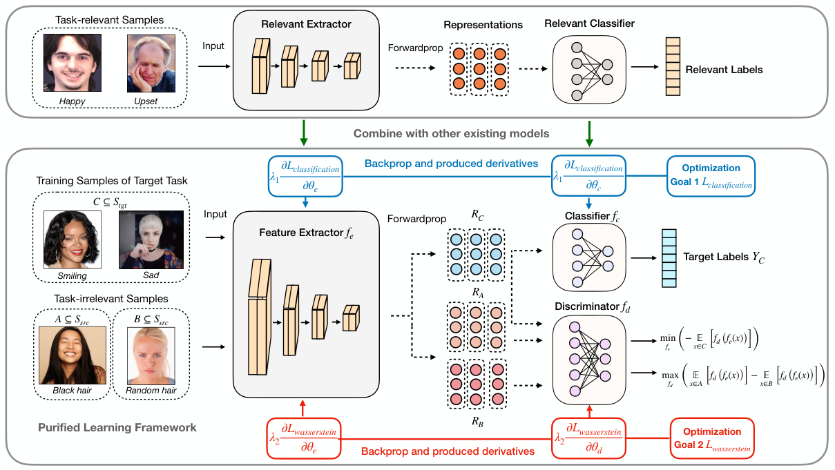
Purified Learning focuses on exploiting the knowledge contained in task-irrelevant labels from auxiliary samples and transferring it to the target task. With this knowledge, we measure the influence of task-irrelevant features, and then use the adversarial learning method based on Wasserstein distances to limit such influence during feature extraction. In this way, original extract features is purified, increasing the percentage of task-relevant features. Generally, the framework is divided into three parts: a feature extractor , a linear classifier and an additional discriminator , as shown in Figure 1. We denote the dataset of the target task by , and the task-irrelevant dataset by . Note that Purified Learning is a theoretically validation framework, the extractor, discriminator and classifier are all flexible and have multiple choices. A practice choice is to set them according to performance. To utilize both and , two optimization goals are set according to Sec. II.
III-A Goal 1: Empirical Risk Minimization
For training sample and label , , the classification probability , and the classification loss is calculated by cross-entropy loss, which is consistent with the loss in empirical risk.
| (18) |
Goal 1 is the empirical risk minimization that we minimize the classification error so that the model learns the knowledge contained in the samples of . However, the generalization ability of the model trained on Goal 1 depends heavily on the consistency of the training data distribution and the real data distribution as we discussed before, which is usually hard to achieve on a small dataset. Thus, a new optimization goal should be imported to utilize large-scale task-relevant or task-irrelevant data to reduce this bias.
III-B Goal 2: Wasserstein Distance Minimization
This goal aims to minimize the Wasserstein distance between and as Equation 6, and it is necessary to estimate the two distributions by sampling. For , we randomly select two groups of samples, one from samples with a specific task-irrelevant label in , denoted by , and the other from the entire , denoted by . For and , the representations extracted by are denoted by , :
| (19) |
Require:
target training sample set ; task-irrelevant sample set ; learning rate for discriminator ; learning rate for feature extractor and classifier ; batch size ; Iteration numbers , .
Notation:
function fitted by the feature extractor, ; function fitted by the classifier, ; function fitted by the discriminator, .
When the sizes of and are large enough, the representation distributions of and , denoted by and , are used as reasonable estimations of and . Thus, Equation 6 is rewritten as:
| (20) |
We substitute the with Wasserstein’s Kantorovich-Rubinstein duality form,
| (21) |
Inspired by WGAN [3], Equation 21 could be divided into two steps. Firstly, the discriminator is trained by:
| (22) |
Secondly, we select a group of training samples, , from training dataset of target task . The feature representations extracted by are denoted by ,
| (23) |
then, the extractor is trained by:
| (24) |
and the corresponding Wasserstein loss is:
| (25) |
where is the size of the sample group C.
Combining and , the complete loss function is written as follows, where are weighting factors:
| (26) |
In practice, the training algorithm is shown in Alg. 1.
IV Experiments
| Feature Extractor | Train Test Dataset | Goal 1 Only |
|
|
|
| ||||||||
|---|---|---|---|---|---|---|---|---|---|---|---|---|---|---|
| AlexNet | ck+ mmi | 35.91 | 38.28 | 33.73 | 34.57 | 37.61 | ||||||||
| ck+ oulu | 34.75 | 25.54 | 33.08 | 33.15 | 38.31 | |||||||||
| mmi ck+ | 56.36 | 44.97 | 57.09 | 57.94 | 61.45 | |||||||||
| mmi oulu | 22.12 | 19.89 | 23.66 | 28.73 | 22.61 | |||||||||
| oulu ck+ | 55.03 | 54.42 | 54.67 | 43.52 | 59.64 | |||||||||
| oulu mmi | 39.46 | 40.00 | 40.30 | 28.33 | 45.36 | |||||||||
| Average | 40.61 | 37.18 | 40.42 | 37.37 | 44.16 | |||||||||
| ResNet34 | ck+ mmi | 50.42 | 46.54 | 46.54 | 44.35 | 50.42 | ||||||||
| ck+ oulu | 50.94 | 54.29 | 47.24 | 43.75 | 51.78 | |||||||||
| mmi ck+ | 65.33 | 68.73 | 66.18 | 64.61 | 69.21 | |||||||||
| mmi oulu | 44.87 | 46.13 | 40.96 | 42.15 | 42.43 | |||||||||
| oulu ck+ | 73.45 | 73.33 | 72.93 | 66.18 | 80.12 | |||||||||
| oulu mmi | 54.13 | 49.01 | 51.43 | 41.99 | 54.30 | |||||||||
| Average | 56.52 | 56.34 | 54.21 | 50.51 | 58.04 | |||||||||
| VggNet19 | ck+ mmi | 45.53 | 41.10 | 37.10 | 33.05 | 45.53 | ||||||||
| ck+ oulu | 56.66 | 44.52 | 32.24 | 47.66 | 57.22 | |||||||||
| mmi ck+ | 65.33 | 62.30 | 64.61 | 57.82 | 66.79 | |||||||||
| mmi oulu | 45.08 | 32.17 | 46.69 | 40.20 | 46.76 | |||||||||
| oulu ck+ | 76.73 | 71.27 | 72.12 | 31.88 | 78.91 | |||||||||
| oulu mmi | 45.03 | 43.68 | 40.00 | 20.24 | 51.43 | |||||||||
| Average | 55.73 | 49.17 | 48.79 | 38.48 | 57.77 |
IV-A Experimental Setup
IV-A1 Model
As mentioned before, the framework of Purified Learning consists of three parts: a feature extractor, a linear classifier, and a discriminator. The discriminator consists of four fully connected layers. The linear classifier is a fully connected layer with the number of neurons depending on the specific task. The flexibity of Purified Learning enables that various mainstream models can be embed as feature extractor.
IV-A2 Evaluation Metrics
To evaluate the results of model generalization, the cross-dataset test results are taken as evaluation metrics. This is based on a reasonable assumption: the training set and the real data distribution are different, and the unseen test set is sampled from the real data distribution, so there exists a gap between the distribution of test data and that of training data. Therefore, the higher the accuracy in our test means the better the generalization performance of the model.
IV-A3 Hyperparameters
We implement all experiments without data augmentation. The model is trained by an SGD optimizer with an initial learning rate of 0.001, the momentum of 0.9, StepLR(step size is 7), and of 0.1. We apply widely used classification models (e.g ResNet) as a feature extractor and set the output dimension of the penultimate layer to 128. The classifier is a fully connected layer and the output dimension is equal to the number of classes (7 for FER and 10 for digit recognition). The discriminator consists of four fully connected layers with 512, 256, 10, 1 nodes, the discriminator is trained using an Adam with the same learning rate, and a weight limit 0.1. In addition, the step ratio of in Alg.1 is 3. The factors and are both 1. We use batch size 32 in FER, and 128 in digit recognition. All results are obtained after the model has been trained for 50 epochs.
IV-B Experimental implementation details
We provide implementation details of the comparison method used in our experiments.
IV-B1 Facial Expression Recognition
- •
Transfer learning: We adopt the pre-training/fine-tuning approaches to transfer learning based on shared parameters [37]. We first pre-train the feature extractor as well as the classifier on CelebA for hair color classification and then train the whole model on the expression dataset.
- •
Multi-task learning: We adopt the multi-task learning approach with hard parameter sharing of hidden layers [5]. Specifically, a shared feature extractor accepts both images with hair color tags from CelebA and images with expression tags from a training set. And two independent classifier networks make separate predictions for hair color and expressions. The entire network gets trained by backpropagating the final loss which is calculated by adding up the classification loss of hair color and the classification loss of expression.
- •
Adversarial Multi-task Learning: Based on the multi-tasking learning model, a new gradient reversal layer (GRL) is added between the feature extractor and the hair color classifier, where the idea is consistent with Shinohara [27].
IV-B2 Digit Recognition
- •
DANN: DANN is a framework for unsupervised domain adaptation based on adversarial multitasking learning proposed by Ganin [8]. As a comparison method for the simultaneous use of MNIST and SVHN data, it is implemented by adding a new gradient reversal layer (GRL) and a domain classifier with 2-dimensional outputs for domain classification to the existing feature extractor and classifier. The feature extractor accepts both images from MNIST and SVHN. One classifier then classifies the feature representation of the MNIST data from 0 to 9, and another classifier distinguishes whether the feature representation originates from MNIST or SVHN.
IV-C Experiments on Facial Expression Recognition
In this part, we compare Purified Learning with some methods related to our work on the FER task. These methods are briefly described below, and their implementation details are shown in Section IV-B:
- •
Goal 1 Only: As an empirical baseline, we use labeled training data to train the model with the optimization goal 1 only.
- •
Transfer learning : We use the hair color recognition task to pre-train the network, and then fine-tune on FER task.
- •
Multi-task learning : We train FER and hair color recognition tasks using a shared feature extractor.
- •
Adversarial multi-task learning: We add a gradient inversion layer for the hair color recognition task on the multi-task learning method above.
IV-C1 Datasets and Feature Extractors
In FER experiments, we use small-scale datasets, including ck+ [16], oulu [41] and mmi [21] for cross-dataset evaluation. We select AlexNet [13], VggNet19 [28] and ResNet34 [10] as feature extractors.
We use resolution for all RGB pictures and preprocess them through MTCNN [38] for alignment. More importantly, the hair color label in CelebA [15] is regarded as task-irrelevant label. Therefore, we select samples with fixed hair color labels and samples randomly selected from CelebA, and then using Purified Learning on them.
IV-C2 Results
Table I is the comparison between Purified Learning and baseline methods, which shows that our method achieves better results in 14 of 18 cross-dataset tests.
Since hair color is not relevant to FER, it leads to negative transfer for transfer learning methods including transfer learning, multi-task learning and adversarial multi-task learning (lower accuracy even than Goal 1 Only in most cases). The performance of the adversarial multi-task learning is the worst because it requires training samples with both task label and task-irrelevant label. However, in our experiments, the training samples are only annotated with task labels, and the task-irrelevant labels are from additional samples. By contrast, Purified Learning is able to make use of the knowledge from task-irrelevant labels, so it improves the accuracy of Goal 1 only, thus successfully resolving negative transfer and improving the generalization performance of the model.
IV-D Experiments on Digit Recognition
In this part, we evaluate Purified Learning on Digit Recognition task. In this experiment, we add another baseline, DANN [1], a domain transfer framework based on adversarial multi-task learning. DANN is currently the state-of-the-art method of transferring from MNIST to MNIST-M11 1 Link to Paperwithcode. Since we use small-scale training set, our accuracy is lower than original paper. The model details of DANN have been shown in Section IV-B.
IV-D1 Datasets and Feature Extractors
In the digit recognition experiments, regarding background color as the task-irrelevant features, we also use a small-scale training set, which are 20000 pictures selected from MNIST [14]. The test sets are SVHN [20] and MNIST-M [8]. The two groups of samples are randomly sampled from MNIST and the combination of MNIST and SVHN respectively. Besides, all pictures are converted to RGB pictures and we use resolution.
IV-D2 Results
|
|
|
DANN |
| ||||||||
|---|---|---|---|---|---|---|---|---|---|---|---|---|
| MNIST SVHN | DenseNet121 | 13.85 | 10.64 | 16.44 | ||||||||
| EfficientNet | 22.99 | 13.99 | 33.74 | |||||||||
| MobileNetV2 | 20.06 | 11.35 | 22.11 | |||||||||
| ResNet18 | 15.01 | 12.00 | 18.83 | |||||||||
| SeNet | 15.44 | 10.69 | 18.22 | |||||||||
| ShuffleNetV2 | 14.29 | 11.98 | 20.72 | |||||||||
| VggNet11 | 19.50 | 13.79 | 25.71 | |||||||||
| Average | 17.31 | 12.06 | 22.25 | |||||||||
| MNIST MNIST-M | DenseNet121 | 25.26 | 14.28 | 35.21 | ||||||||
| EfficientNet | 40.78 | 38.71 | 57.64 | |||||||||
| MobileNetV2 | 29.77 | 21.75 | 48.76 | |||||||||
| ResNet18 | 25.10 | 22.54 | 37.64 | |||||||||
| SeNet | 17.24 | 15.83 | 39.71 | |||||||||
| ShuffleNetV2 | 27.96 | 20.34 | 47.65 | |||||||||
| VggNet11 | 39.18 | 42.09 | 48.98 | |||||||||
| Average | 29.33 | 25.08 | 45.08 |
Table II is the comparison between our method and two baselines. Compared with baselines, Purified Learning achieves higher accuracy than DANN and Goal 1 Only method. The Although transferring from MNIST to SVHN is difficult since SVHN is much more complex than MNIST, Purified Learning improves DANN by more than 10% accuracy, which proves the effectiveness of using task-irrelevant features. We also achieve better results than DANN in the “MNIST to MNIST-M” task.
IV-E Discussion
IV-E1 The impact of different levels of task-irrelevance.
|
|
|
|
| ||||||||||
|---|---|---|---|---|---|---|---|---|---|---|---|---|---|---|
| AlexNet | ck+ mmi | 35.91 | 32.38 | 37.61 | ||||||||||
| ck+ oulu | 34.75 | 33.91 | 38.31 | |||||||||||
| mmi ck+ | 56.36 | 35.39 | 61.45 | |||||||||||
| mmi oulu | 22.12 | 18.77 | 22.61 | |||||||||||
| oulu ck+ | 55.03 | 49.33 | 59.64 | |||||||||||
| oulu mmi | 39.46 | 38.45 | 45.36 | |||||||||||
| Average | 40.61 | 34.71 | 44.16 | |||||||||||
| ResNet34 | ck+ mmi | 50.42 | 47.89 | 50.42 | ||||||||||
| ck+ oulu | 50.94 | 50.31 | 51.78 | |||||||||||
| mmi ck+ | 65.33 | 65.70 | 69.21 | |||||||||||
| mmi oulu | 44.87 | 39.22 | 42.43 | |||||||||||
| oulu ck+ | 73.45 | 73.70 | 80.12 | |||||||||||
| oulu mmi | 54.13 | 51.43 | 54.30 | |||||||||||
| Average | 56.52 | 54.71 | 58.04 | |||||||||||
| VggNet19 | ck+ mmi | 45.53 | 40.47 | 45.53 | ||||||||||
| ck+ oulu | 56.66 | 42.99 | 57.22 | |||||||||||
| mmi ck+ | 65.33 | 63.64 | 66.79 | |||||||||||
| mmi oulu | 45.08 | 44.59 | 46.76 | |||||||||||
| oulu ck+ | 76.73 | 75.03 | 78.91 | |||||||||||
| oulu mmi | 45.03 | 50.59 | 51.43 | |||||||||||
| Average | 55.73 | 52.89 | 57.77 |
As different task-relevance can affect the performance of transfer learning, it is essential to study the impact of different levels of task-irrelevance on Purified Learning. Except for the hair color label, we use the smiling label from CelebA. We apply these labels to the Purified Learning framework and compare their performance.
Table III indicates that the experiment results that compared with Goal 1 Only method, the performance of Purified Learning remains the same or gets worse when using the smiling label, but have significant improvement when using the hair color label. The experiment results suggest that using a more irrelevant label is better for the Purified Learning framework to improve the performance since it tries to use the knowledge of task-irrelevant features. On the other hand, if we misuse task-relevant samples in Purified Learning, it will have a negative impact. This is similar to negative transfer while using task-irrelevant labels in transfer learning. In general, this phenomenon means that Purified Learning differs from transfer learning, since it benefits from the irrelevance of data instead of relevance.
IV-E2 PCA analysis on feature representations
Based on the maximum variance theory [30], if the percentage of variance explained by principal components increase, the representation vector will contain more information about task-relevant features, and task-relevant information will be better retained during the process of dimension reduction.
Figure 2 shows the proportion of principal components of different methods in digit recognition tasks. Compared with other methods (Goal 1 Only and DANN), the proportion of task-relevant information is significantly higher in Purified Learning, which means that Purified Learning learns knowledge from task-irrelevant labels and avoid extracting task-irrelevant features during feature extraction.
V Conclusion
In this paper, we propose a novel framework, Purified Learning, to exploit the knowledge from additional task-irrelevant labels in order to solve the problem caused by the unreliable empirical risk minimization when the training dataset is small. Based on detailed theoretical analysis, we illustrate that samples with task-irrelevant labels can be used in improving the generalization performance of the model, based on which we propose Purified Learning, which directly obtains and utilizes knowledge from a wide range of task-irrelevant labels. Furthermore, Purified Learning can be well combined with the existing task-relevant learning methods. We believe that the exploration of task-irrelevant labels in our work provides a valuable insight for future research.
VI Acknowledgement
This research is supported by National Natural Science Foundation of China (Grant No. 6201101015 and 61602013), Beijing Academy of Artificial Intelligence (BAAI), the Natural Science Foundation of Guangdong Province (Grant No. 2021A1515012640), the Basic Research Fund of Shenzhen City (Grant No. JCYJ20210324120012033 and JCYJ20190813165003837), the Shenzhen General Research Project (Grant No. JCYJ20190808182805919), the National Key R&D Program of China (No. 2021ZD0112905), the Overseas Cooperation Research Fund of Tsinghua Shenzhen International Graduate School (Grant No. HW2021008) and the 173 program (Grant No. 2021-JCJQ-JJ-0029).
References
- [1] H. Ajakan, P. Germain, H. Larochelle, F. Laviolette, and M. Marchand, “Domain-adversarial neural networks,” arXiv preprint arXiv:1412.4446, 2014.
- [2] A. Ajiboye, R. Abdullah-Arshah, and Q. Hongwu, “Evaluating the effect of dataset size on predictive model using supervised learning technique,” 2015.
- [3] M. Arjovsky, S. Chintala, and L. Bottou, “Wasserstein gan,” arXiv preprint arXiv:1701.07875, 2017.
- [4] C. Bowles, L. Chen, R. Guerrero, P. Bentley, R. Gunn, A. Hammers, D. A. Dickie, M. V. Hernández, J. Wardlaw, and D. Rueckert, “Gan augmentation: Augmenting training data using generative adversarial networks,” arXiv preprint arXiv:1810.10863, 2018.
- [5] R. Caruana, “Multitask learning: A knowledge-based source of inductive bias,” in Proceedings of the Tenth International Conference on Machine Learning. Morgan Kaufmann, 1993, pp. 41–48.
- [6] T. Chen, S. Kornblith, M. Norouzi, and G. Hinton, “A simple framework for contrastive learning of visual representations,” arXiv preprint arXiv:2002.05709, 2020.
- [7] E. D. Cubuk, B. Zoph, D. Mane, V. Vasudevan, and Q. V. Le, “Autoaugment: Learning augmentation policies from data,” arXiv preprint arXiv:1805.09501, 2018.
- [8] Y. Ganin, E. Ustinova, H. Ajakan, P. Germain, H. Larochelle, F. Laviolette, M. Marchand, and V. Lempitsky, “Domain-adversarial training of neural networks,” The Journal of Machine Learning Research, vol. 17, no. 1, pp. 2096–2030, 2016.
- [9] J. Gu, Z. Wang, J. Kuen, L. Ma, A. Shahroudy, B. Shuai, T. Liu, X. Wang, G. Wang, J. Cai et al., “Recent advances in convolutional neural networks,” Pattern Recognition, vol. 77, pp. 354–377, 2018.
- [10] K. He, X. Zhang, S. Ren, and J. Sun, “Deep residual learning for image recognition,” in Proceedings of the IEEE conference on computer vision and pattern recognition, 2016, pp. 770–778.
- [11] J. Hu, L. Shen, and G. Sun, “Squeeze-and-excitation networks,” in Proceedings of the IEEE conference on computer vision and pattern recognition, 2018, pp. 7132–7141.
- [12] G. Huang, Z. Liu, L. Van Der Maaten, and K. Q. Weinberger, “Densely connected convolutional networks,” in Proceedings of the IEEE conference on computer vision and pattern recognition, 2017, pp. 4700–4708.
- [13] A. Krizhevsky, I. Sutskever, and G. E. Hinton, “Imagenet classification with deep convolutional neural networks,” in Advances in neural information processing systems, 2012, pp. 1097–1105.
- [14] Y. LeCun, L. Bottou, Y. Bengio, and P. Haffner, “Gradient-based learning applied to document recognition,” Proceedings of the IEEE, vol. 86, no. 11, pp. 2278–2324, 1998.
- [15] Z. Liu, P. Luo, X. Wang, and X. Tang, “Deep learning face attributes in the wild,” in Proceedings of International Conference on Computer Vision (ICCV), December 2015.
- [16] P. Lucey, J. F. Cohn, T. Kanade, J. Saragih, Z. Ambadar, and I. Matthews, “The extended cohn-kanade dataset (ck+): A complete dataset for action unit and emotion-specified expression,” in 2010 ieee computer society conference on computer vision and pattern recognition-workshops. IEEE, 2010, pp. 94–101.
- [17] Z. Luo, Y. Zou, J. Hoffman, and L. F. Fei-Fei, “Label efficient learning of transferable representations acrosss domains and tasks,” in Advances in Neural Information Processing Systems, 2017, pp. 165–177.
- [18] N. Ma, X. Zhang, H.-T. Zheng, and J. Sun, “Shufflenet v2: Practical guidelines for efficient cnn architecture design,” in Proceedings of the European conference on computer vision (ECCV), 2018, pp. 116–131.
- [19] M. Mohri, A. Rostamizadeh, and A. Talwalkar, Foundations of Machine Learning, ser. Adaptive computation and machine learning. MIT Press, 2012.
- [20] Y. Netzer, T. Wang, A. Coates, A. Bissacco, B. Wu, and A. Y. Ng, “Reading digits in natural images with unsupervised feature learning,” 2011.
- [21] M. Pantic, M. Valstar, R. Rademaker, and L. Maat, “Web-based database for facial expression analysis,” in 2005 IEEE international conference on multimedia and Expo. IEEE, 2005, pp. 5–pp.
- [22] J. Prusa, T. M. Khoshgoftaar, and N. Seliya, “The effect of dataset size on training tweet sentiment classifiers,” in 2015 IEEE 14th International Conference on Machine Learning and Applications (ICMLA). IEEE, 2015, pp. 96–102.
- [23] M. T. Rosenstein, Z. Marx, L. P. Kaelbling, and T. G. Dietterich, “To transfer or not to transfer,” in NIPS 2005 workshop on transfer learning, vol. 898, 2005, pp. 1–4.
- [24] M. Sandler, A. Howard, M. Zhu, A. Zhmoginov, and L.-C. Chen, “Mobilenetv2: Inverted residuals and linear bottlenecks,” in Proceedings of the IEEE conference on computer vision and pattern recognition, 2018, pp. 4510–4520.
- [25] J. Shen, Y. Qu, W. Zhang, and Y. Yu, “Wasserstein distance guided representation learning for domain adaptation,” arXiv preprint arXiv:1707.01217, 2017.
- [26] Y. Shinohara, “Adversarial multi-task learning of deep neural networks for robust speech recognition.” in Interspeech. San Francisco, CA, USA, 2016, pp. 2369–2372.
- [27] ——, “Adversarial multi-task learning of deep neural networks for robust speech recognition.” in Interspeech. San Francisco, CA, USA, 2016, pp. 2369–2372.
- [28] K. Simonyan and A. Zisserman, “Very deep convolutional networks for large-scale image recognition,” in International Conference on Learning Representations, 2015.
- [29] M. Tan and Q. V. Le, “Efficientnet: Rethinking model scaling for convolutional neural networks,” arXiv preprint arXiv:1905.11946, 2019.
- [30] M. E. Tipping and C. M. Bishop, “Mixtures of probabilistic principal component analyzers,” Neural computation, vol. 11, no. 2, pp. 443–482, 1999.
- [31] T. Tommasi, N. Patricia, B. Caputo, and T. Tuytelaars, “A deeper look at dataset bias,” in Domain adaptation in computer vision applications. Springer, 2017, pp. 37–55.
- [32] A. Torralba and A. A. Efros, “Unbiased look at dataset bias,” in CVPR 2011. IEEE, 2011, pp. 1521–1528.
- [33] V. Vapnik, “Principles of risk minimization for learning theory,” in Advances in Neural Information Processing Systems 4, [NIPS Conference, Denver, Colorado, USA, December 2-5, 1991], J. E. Moody, S. J. Hanson, and R. Lippmann, Eds. Morgan Kaufmann, 1991, pp. 831–838.
- [34] Y. Wang, Q. Yao, J. T. Kwok, and L. M. Ni, “Generalizing from a few examples: A survey on few-shot learning,” ACM Computing Surveys (CSUR), vol. 53, no. 3, pp. 1–34, 2020.
- [35] Y.-X. Wang and M. Hebert, “Learning to learn: Model regression networks for easy small sample learning,” in European Conference on Computer Vision. Springer, 2016, pp. 616–634.
- [36] K. Weiss, T. M. Khoshgoftaar, and D. Wang, “A survey of transfer learning,” Journal of Big data, vol. 3, no. 1, p. 9, 2016.
- [37] J. Yosinski, J. Clune, Y. Bengio, and H. Lipson, “How transferable are features in deep neural networks?” in Advances in neural information processing systems, 2014, pp. 3320–3328.
- [38] K. Zhang, Z. Zhang, Z. Li, and Y. Qiao, “Joint face detection and alignment using multitask cascaded convolutional networks,” IEEE Signal Processing Letters, vol. 23, no. 10, pp. 1499–1503, 2016.
- [39] X. Zhang, Z. Wang, D. Liu, Q. Lin, and Q. Ling, “Deep adversarial data augmentation for extremely low data regimes,” IEEE Transactions on Circuits and Systems for Video Technology, 2020.
- [40] Z. Zhang, P. Luo, C. C. Loy, and X. Tang, “Facial landmark detection by deep multi-task learning,” in European conference on computer vision. Springer, 2014, pp. 94–108.
- [41] G. Zhao, X. Huang, M. Taini, S. Z. Li, and M. PietikäInen, “Facial expression recognition from near-infrared videos,” Image and Vision Computing, vol. 29, no. 9, pp. 607–619, 2011.