跳到论文正文
W Papers独立论文阅读器 arXiv:2102.10941 论文正文 计算阅读时间 · 0%
引用这篇论文根据当前论文元数据生成,正式投稿前建议核对。


License: arXiv.org perpetual non-exclusive license
arXiv:2102.10941v1 [math.NA] 22 Feb 2021

Singular Euler–Maclaurin expansion on multidimensional lattices

Andreas A. Buchheit Address: Department of Mathematics, Saarland University, PO 15 11 50, D-66041 Saarbrücken Email address: buchheit@num.uni-sb.de and Torsten Keßler Address: Department of Mathematics, Saarland University, PO 15 11 50, D-66041 Saarbrücken Email address: kessler@num.uni-sb.de
Abstract.

We extend the classical Euler–Maclaurin expansion to sums over multidimensional lattices that involve functions with algebraic singularities. This offers a tool for the precise quantification of the effect of microscopic discreteness on macroscopic properties of a system. First, the Euler–Maclaurin summation formula is generalised to lattices in higher dimensions, assuming a sufficiently regular summand function. We then develop this new expansion further and construct the singular Euler–Maclaurin (SEM) expansion in higher dimensions, an extension of our previous work in one dimension, which remains applicable and useful even if the summand function includes a singular function factor. We connect our method to analytical number theory and show that all operator coefficients can be efficiently computed from derivatives of the Epstein zeta function. Finally we demonstrate the numerical performance of the expansion and efficiently compute singular lattice sums in infinite two-dimensional lattices, which are of high relevance in solid state and quantum physics. An implementation in Mathematica is provided online along with this article.

Key words and phrases:
Euler–Maclaurin expansion, long-range interactions, quadrature, multidimensional lattice sums, partial differential equations, elliptic regularity, analytic number theory
2010 Mathematics Subject Classification
Primary 65B1, 540H05; Secondary 46F10, 35B65, 11E45

1. Introduction

Discrete particle systems with long-range interactions appear abundantly in nature. For instance, the microscopic electromagnetic interactions between atoms and molecules give rise to the macroscopic properties of a solid. The universe itself is composed of subatomic particles and their interactions determine the evolution of the whole. Some theories extend this notion of granularity to space-time itself. In lattice quantum field theories, the discreteness of the space-time regularises divergent path-integrals and simplifies numerical predictions [30]. Other theories employ discreteness at the Planck-scale in order to reconcile quantum mechanics with general relativity, e.g. loop quantum gravity [7, 29]. Recently, it has been conjectured that a granularity of space-time could explain dark energy, the cause for the accelerating expanse of the universe [28].

Finding an efficient way to compute sums with a large number of addends, as they appear for instance in the simulation of discrete particle systems in condensed matter or in the evaluation of partition functions in statistical physics, is in general a challenging task. For instance, the number of summands required in the computation of the energy of a lattice with long-range interactions scales quadratically with the particle number and becomes unfeasible for solid state systems of macroscopic size, where the particle number is in the range of N≈1023N\approx 10^{23}.

A continuum is, in many cases, more accessible than a discrete system. Arising integrals can often be computed analytically or, at least, decent quadrature rules for numeric approximations exist. Moreover, our mathematical understanding of continuous systems vastly exceeds the understanding of discrete systems, a notable exception being the tools developed in number theory. It is thus natural to ask, in how far we can describe a discrete system by a related continuum, or in how far a lattice sum can be approximated by an integral.

The main tool for describing the difference between a sum and an integral in one dimension is the Euler–Maclaurin (EM) expansion (see [2] for a historic overview). For ℓ∈ℕ\ell\in\mathds{N}, a,b∈ℤa,b\in\mathds{Z}, δ1,δ2∈(0,1]\delta_{1},\delta_{2}\in(0,1] and f∈Cℓ+1​([a+δ1,b+δ2],ℂ)f\in C^{\ell+1}([a+\delta_{1},b+\delta_{2}],\mathds{C}), we have [2, 5, 25]

∑y=a+1bf⁡(y)−∫a+δ1b+δ2f⁡(y)​𝑑y=\displaystyle\sum_{y=a+1}^{b}f(y)-\int\limits_{a+\delta_{1}}^{b+\delta_{2}}f(y)\,\mathrm{d}y= −∑k=0ℓ(−1)kk!Bk+1​(1+y−⌈y⌉)k+1f(k)(y)|y=a+δ1y=b+δ2\displaystyle-\sum_{k=0}^{\ell}\frac{(-1)^{k}}{k!}\frac{B_{k+1}(1+y-\lceil y\rceil)}{k+1}f^{(k)}(y)\bigg|^{y=b+\delta_{2}}_{y=a+\delta_{1}}
+(−1)ℓℓ!∫a+δ1b+δ2Bℓ+1​(1+y−⌈y⌉)ℓ+1f(ℓ+1)(y)dy,\displaystyle+\frac{(-1)^{\ell}}{\ell!}\int\limits_{a+\delta_{1}}^{b+\delta_{2}}\frac{B_{\ell+1}(1+y-\lceil y\rceil)}{\ell+1}f^{(\ell+1)}(y)\,\mathrm{d}y,

with ⌈y⌉\lceil y\rceil the ceiling of yy and BℓB_{\ell} the Bernoulli polynomials, which are defined by the recurrence relation

B0(y)=1,B′ℓ(y)=ℓBℓ−1(y),∫01Bℓ(y)dy=0,ℓ≥1.\displaystyle B_{0}(y)=1,\quad B^{\prime}_{\ell}(y)=\ell B_{\ell-1}(y),\quad\int\limits_{0}^{1}B_{\ell}(y)\,\mathrm{d}y=0,\quad\ell\geq 1.

The EM expansion has been extended to higher dimensions, where the main approach is based on a tensorisation of the 1D expansion. For a higher-dimensional equivalent of the EM expansion applicable to polynomials on simple polytopes, see e.g. [22]. Higher dimensional extensions of the EM expansion that do not rely on repeated application of the 1D result are rare, a notable exception being the work by Müller in [26], where a two dimensional generalisation of the EM expansion was derived that is valid for a larger set of functions and integration regions. A second example is the work by Freeden [13] in which a generalisation of the Müller result to higher dimensions has been carried out. The above generalisations of the EM expansion exhibits different advantages and disadvantages. While the results based on tensorisation (or Todd operators) are easy to apply in practice, they are very restrictive in the set of functions and integration regions that are allowed. Also, they usually do not give error estimates. The non-tensorised results apply to a more general set of functions and regions, however, the results are mainly theoretical and error estimates are missing.

All of the above generalisation share one critical disadvantage: They are not applicable to summand functions, whose derivatives increase quickly with the derivative order, e.g. due to an algebraic singularity. Unfortunately, these functions are of high importance in physical applications, as for instance all relevant interparticle interaction, e.g. the Coulomb interaction between charged particles, belong to this set of functions.

In our previous work [5], we have developed the singular Euler–Maclaurin (SEM) expansion that makes the EM expansion applicable to physically relevant summand functions in one-dimension, including functions that exhibit an algebraic singularity. In this paper, we extend our previous work and generalise the SEM expansion from one dimension to lattices in an arbitrary number of space dimensions. We avoid a simple yet restrictive tensorisation of the 1D result, and offer a generalisation of the SEM expansion that can be applied to physically relevant interaction functions and lattice structures. We show that our expansion can be used as a powerful numerical tool for the fast evaluation of forces and energies in lattices of macroscopic size. Furthermore, we are able to precisely determine the effect of a microscopic granularity on a macroscopic system, even if the ratio between the macro and the micro scale is astronomically large.

This work is structured as follows. In Section 2, we provide a short overview on distribution theory and elliptic regularity, which serve as important tools in the following parts. We then derive a generalisation of the EM expansion to multidimensional lattices in Section 3, which is subsequently used as a stepping stone for arriving at the SEM expansion in higher dimensions in Section 4. Here we address first the case that the singularity is positioned at a lattice point outside of the integration region and then move on to the challenging but highly relevant case that it is found inside of it. We then remove the only free parameter of the SEM for interior lattice points in Section 5 by means of hypersingular integrals, which leads to the hypersingular Euler–Maclaurin expansion. During this procedure, we unravel a deep connection of our theory to analytic number theory, which opens a way for us to efficiently compute all necessary operator coefficients. We then demonstrate the numerical performance of the expansion in Section 6 and analyse the error. Finally, we draw our conclusions in Section 7.

2. Preliminaries

In the presentation of the material we mostly follow [20]. An extensively study the Fourier transform and explicit expressions for many distributions can be found in [15]. Finally, the first chapter of [33] presents an accessible introduction to elliptic regularity.

2.1. Distributions

For an open set Ω⊆ℝd\Omega\subseteq\mathds{R}^{d} and k∈ℕ={0,1,2,…}k\in\mathds{N}=\{0,1,2,\dots\} or k=∞k=\infty, Ck​(Ω)C^{k}(\Omega) denotes the set of kk-times continuously differentiable functions f:Ω→ℂf:\Omega\to\mathds{C}. A sequence (un)n∈ℕ(u_{n})_{n\in\mathds{N}} in Ck​(Ω)C^{k}(\Omega) is said to converge to u∈Ck​(Ω)u\in C^{k}(\Omega) if all derivatives up to order kk converge compactly on Ω\Omega, i.e. for all K⊆ΩK\subseteq\Omega compact and 𝜶∈ℕd\bm{\alpha}\in\mathds{N}^{d} with |𝜶|≤k|\bm{\alpha}|\leq k,

limn→∞sup𝒙∈K|D𝜶​un​(𝒙)−D𝜶​u​(𝒙)|=0.\lim_{n\to\infty}\sup_{\bm{x}\in K}\big|D^{\bm{\alpha}}u_{n}(\bm{x})-D^{\bm{\alpha}}u(\bm{x})\big|=0.

With C0k​(Ω)C_{0}^{k}(\Omega) we denote the subspace of functions in u∈Ck​(Ω)u\in C^{k}(\Omega) whose support

suppu={𝒙∈Ω:u⁡(𝒙)≠0}¯\supp u=\overline{\{\bm{x}\in\Omega:u(\bm{x})\neq 0\}}

is contained in a compact subset of Ω\Omega. Endowed with a stronger topology than the one inherited from C∞​(Ω)C^{\infty}(\Omega), C0∞​(Ω)C_{0}^{\infty}(\Omega) is called the space of test functions. Its dual space, denoted by 𝒟′​(Ω)\mathscr{D}^{\prime}(\Omega), is called the space of distributions on Ω\Omega. A prototypical example of a distribution is the Dirac distribution at 𝒙0∈Ω\bm{x}_{0}\in\Omega which sends a test function to its point evaluation in 𝒙0\bm{x}_{0},

⟨δ𝒙0,ψ⟩=ψ⁡(𝒙0),ψ∈C0∞​(Ω).\langle\delta_{\bm{x}_{0}},\psi\rangle=\psi(\bm{x}_{0}),\quad\psi\in C_{0}^{\infty}(\Omega).

For p∈[1,∞]p\in[1,\infty], we set Lp​(Ω)L^{p}(\Omega) as the Banach space of all measurable functions v:Ω→ℂv:\Omega\to\mathds{C} with finite pp-norm,

‖v‖p,Ωp=∫Ω|v⁡(𝒙)|p​d​𝒙<∞,\|v\|_{p,\Omega}^{p}=\int\limits_{\Omega}|v(\bm{x})|^{p}\,\text{d}\bm{x}<\infty,

for p<∞p<\infty and

‖v‖∞,Ω=ess​sup𝒙∈Ω⁡|v⁡(𝒙)|<∞,\|v\|_{\infty,\Omega}=\operatorname*{ess\,sup}_{\bm{x}\in\Omega}|v(\bm{x})|<\infty,

in case of p=∞p=\infty. Furthermore, the space of locally pp-integrable functions is defined as

Llocp(Ω)={v:Ω→ℂ measurable :v|K∈Lp(K) for all K⊆Ω compact}.L_{\text{loc}}^{p}(\Omega)=\big\{v:\Omega\to\mathds{C}\text{ measurable }:v|_{K}\in L^{p}(K)\text{ for all }K\subseteq\Omega\text{ compact}\big\}.

Every function v∈Lloc1​(Ω)v\in L^{1}_{\text{loc}}(\Omega) defines a distribution by virtue of

C0∞​(Ω)→ℂ,ψ↦∫Ωv⁡(𝒙)​ψ​(𝒙)​d​𝒙.C_{0}^{\infty}(\Omega)\to\mathds{C},\penalty\ \psi\mapsto\int\limits_{\Omega}v(\bm{x})\psi(\bm{x})\,\text{d}\bm{x}.

Of particular interest for us are the functions sν:ℝd∖{𝟎}→ℂs_{\nu}:\mathds{R}^{d}\setminus\{\bm{0}\}\to\mathds{C},

(2.1) sν​(𝒙)=1|𝒙|ν,s_{\nu}(\bm{x})=\frac{1}{|\bm{x}|^{\nu}},

for ν∈ℂ\nu\in\mathds{C}. Clearly, sνs_{\nu} gives rise to a distribution on ℝd∖{𝟎}\mathds{R}^{d}\setminus\{\bm{0}\}. Additionally, we have

Theorem 2.1.

The function sνs_{\nu} has an extension to a distribution on ℝd\mathds{R}^{d}. In case that ν≠d+2​k\nu\neq d+2k, k∈ℕk\in\mathds{N} this extension is unique. Otherwise, for ν=d+2​k\nu=d+2k, there are infinitely many extensions and two of them differ by a linear combination of derivatives of order kk of δ𝟎\delta_{\bm{0}}.

We denote the convolution of u∈𝒟′​(ℝd)u\in\mathscr{D}^{\prime}(\mathds{R}^{d}) and φ∈C∞​(ℝd)\varphi\in C^{\infty}(\mathds{R}^{d}), where one of them is assumed to have compact support, by u∗φu\ast\varphi. It holds u∗φ∈C∞​(ℝd)u\ast\varphi\in C^{\infty}(\mathds{R}^{d}) and

(u∗φ)(𝒙)=u(φ(𝒙−⋅)),𝒙∈ℝd.(u\ast\varphi)(\bm{x})=u(\varphi(\bm{x}-\bm{\cdot})),\quad\bm{x}\in\mathds{R}^{d}.

For v∈L1​(ℝd)v\in L^{1}(\mathds{R}^{d}), we define the Fourier transform v^=ℱ​v\hat{v}=\mathcal{F}v as

v^​(𝝃)=ℱ​v​(𝝃)=∫ℝde−2​π​i​⟨𝝃,𝒙⟩​v​(𝒙)​d​𝒙,𝝃∈ℝd.\hat{v}(\bm{\xi})=\mathcal{F}v(\bm{\xi})=\int\limits_{\mathds{R}^{d}}e^{-2\pi i\langle\bm{\xi},\bm{x}\rangle}v(\bm{x})\,\text{d}\bm{x},\quad\bm{\xi}\in\mathds{R}^{d}.

The Fourier transform is an isomorphism on the Schwartz space S⁡(ℝd)S(\mathds{R}^{d}) of rapidly decaying smooth functions,

S(ℝd)={u∈C∞(ℝd):sup𝒙∈ℝd|𝒙𝜷D𝜶u(𝒙)|<∞∀𝜶,𝜷∈ℕd}.S(\mathds{R}^{d})=\Big\{u\in C^{\infty}(\mathds{R}^{d}):\sup_{\bm{x}\in\mathds{R}^{d}}|\bm{x}^{\bm{\beta}}D^{\bm{\alpha}}u(\bm{x})|<\infty\penalty\ \forall\bm{\alpha},\bm{\beta}\in\mathds{N}^{d}\Big\}.

By duality, the definition of ℱ\mathcal{F} extends to S′​(ℝd)S^{\prime}(\mathds{R}^{d}), the dual space of S⁡(ℝd)S(\mathds{R}^{d}), called the space of tempered distributions.

Theorem 2.2.

Let ν∈ℂ\nu\in\mathds{C}. Any extension of sνs_{\nu} to a distribution on ℝd\mathds{R}^{d} is a tempered distribution. Its Fourier transform is a C∞C^{\infty}-function on ℝd∖{𝟎}\mathds{R}^{d}\setminus\{\bm{0}\}. For ν∉(d+2​ℕ)\nu\not\in(d+2\mathds{N}) it holds

s^ν​(𝝃)=πν−d2​Γ⁡(d−ν2)Γ⁡(ν2)​|𝝃|−d+ν,𝝃∈ℝd∖{𝟎},\hat{s}_{\nu}(\bm{\xi})=\pi^{\nu-\frac{d}{2}}\frac{\Gamma\big(\frac{d-\nu}{2}\big)}{\Gamma\big(\frac{\nu}{2}\big)}|\bm{\xi}|^{-d+\nu},\quad\bm{\xi}\in\mathds{R}^{d}\setminus\{\bm{0}\},

where Γ\Gamma denotes the Gamma function.

2.2. Elliptic regularity

A dd-variate polynomial PP of degree m∈ℕm\in\mathds{N} with complex coefficients,

P⁡(𝝃)=∑𝜶∈ℕda𝜶​𝝃𝜶,𝝃∈ℝd,P(\bm{\xi})=\sum_{\bm{\alpha}\in\mathds{N}^{d}}a_{\bm{\alpha}}\bm{\xi}^{\bm{\alpha}},\quad\bm{\xi}\in\mathds{R}^{d},

is called elliptic if

Pm​(𝝃)=∑|𝜶|=ma𝜶​𝝃𝜶,𝝃∈ℝd,P_{m}(\bm{\xi})=\sum_{|\bm{\alpha}|=m}a_{\bm{\alpha}}\bm{\xi}^{\bm{\alpha}},\quad\bm{\xi}\in\mathds{R}^{d},

does not vanish on ℝd∖{𝟎}\mathds{R}^{d}\setminus\{\bm{0}\}. Moreover, a differential operator with constant coefficients is called elliptic if the associated polynomial is elliptic.

Theorem 2.3.

An elliptic differential operator ℒ\mathcal{L} with constant coefficients is hypoelliptic, which means that if ℒ​u∈C∞​(Ω)\mathcal{L}u\in C^{\infty}(\Omega) for u∈𝒟′​(Ω)u\in\mathscr{D}^{\prime}(\Omega), then already u∈C∞​(Ω)u\in C^{\infty}(\Omega).

Theorem 2.3 remains valid if smoothness is replaced by analyticity.

Theorem 2.4.

An elliptic differential operator ℒ\mathcal{L} with constant coefficients is analytic-hypoelliptic: If ℒ​u\mathcal{L}u is analytic in Ω\Omega for u∈𝒟′​(Ω)u\in\mathscr{D}^{\prime}(\Omega), then uu is an analytic function on Ω\Omega.

The following theorem is a generalisation of [20, Theorem 4.4.2].

Theorem 2.5.

Let (uj)j∈ℕ(u_{j})_{j\in\mathds{N}} be a sequence in 𝒟′​(Ω)\mathscr{D}^{\prime}(\Omega) that converges to u∈𝒟′​(Ω)u\in\mathscr{D}^{\prime}(\Omega),

limj→∞uj​(ψ)=u⁡(ψ),ψ∈C0∞​(Ω).\lim_{j\to\infty}u_{j}(\psi)=u(\psi),\quad\psi\in C_{0}^{\infty}(\Omega).

Furthermore, let ℒ\mathcal{L} be an elliptic differential operator with constant coefficients. If we have ℒ​uj∈C∞​(Ω)\mathcal{L}u_{j}\in C^{\infty}(\Omega) for all j∈ℕj\in\mathds{N} and the sequence (ℒ​uj)j∈ℕ(\mathcal{L}u_{j})_{j\in\mathds{N}} converges in C∞​(Ω)C^{\infty}(\Omega) to v∈C∞​(Ω)v\in C^{\infty}(\Omega), then (uj)j∈ℕ(u_{j})_{j\in\mathds{N}} and uu are C∞C^{\infty}-functions and (uj)j∈ℕ(u_{j})_{j\in\mathds{N}} converges to uu in C∞​(Ω)C^{\infty}(\Omega), that is compactly on Ω\Omega in all derivatives.

Proof.

Since ℒ​uj∈C∞​(Ω)\mathcal{L}u_{j}\in C^{\infty}(\Omega) for all j∈ℕj\in\mathds{N} and

ℒ​u=limj→∞ℒ​uj=v​in​𝒟′​(Ω),\mathcal{L}u=\lim_{j\to\infty}\mathcal{L}u_{j}=v\penalty\ \mathrm{in}\penalty\ \mathscr{D}^{\prime}(\Omega),

Theorem 2.3 holds uj∈C∞​(Ω)u_{j}\in C^{\infty}(\Omega) and u∈C∞​(Ω)u\in C^{\infty}(\Omega). We now show that already

limj→∞uj=u​in​C∞​(Ω).\lim_{j\to\infty}u_{j}=u\penalty\ \mathrm{in}\penalty\ C^{\infty}(\Omega).

We first choose an open neighbourhood Y⊆ΩY\subseteq\Omega of KK such that there is χ∈C0∞​(Ω)\chi\in C_{0}^{\infty}(\Omega) with χ=1\chi=1 on YY. Let E∈𝒟′​(Ω)E\in\mathscr{D}^{\prime}(\Omega) be the fundamental solution of ℒ\mathcal{L} which exists by Theorem 7.3.10 in [20]. If we write fj=ℒ​ujf_{j}=\mathcal{L}u_{j} and f=ℒ​uf=\mathcal{L}u, then

uj−u=(uj−E∗(χ​fj))−(u−E∗(χ​f))+E∗(χ⋅(fj−f)).u_{j}-u=\big(u_{j}-E\ast(\chi f_{j})\big)-\big(u-E\ast(\chi f)\big)+E\ast\big(\chi\cdot(f_{j}-f)\big).

On YY, we have

ℒ⁡(uj−E∗(χ​fj))=fj−χ​fj=0.\mathcal{L}\big(u_{j}-E\ast(\chi f_{j})\big)=f_{j}-\chi f_{j}=0.

Furthermore, since the convolution

E∗⋅:C0∞(Ω)→C∞(Ω)E\ast\cdot:C_{0}^{\infty}(\Omega)\to C^{\infty}(\Omega)

is continuous [32, Theorem 27.3], it holds

limj→∞(uj−E∗(χ​fj))=u−E∗(χ​f)​in​𝒟′​(Y).\lim_{j\to\infty}\big(u_{j}-E\ast(\chi f_{j})\big)=u-E\ast(\chi f)\penalty\ \mathrm{in}\penalty\ \mathscr{D}^{\prime}(Y).

By [20, Theorem 4.4.2], above limit also holds in C∞​(Y)C^{\infty}(Y). Again, by using the continuity of the convolution, we conclude that

limj→∞E∗(χ⋅(fj−f))=0​in​C∞​(Y).\lim_{j\to\infty}E\ast\big(\chi\cdot(f_{j}-f)\big)=0\penalty\ \mathrm{in}\penalty\ C^{\infty}(Y).

Therefore, for all 𝜶∈ℕd\bm{\alpha}\in\mathds{N}^{d},

D𝜶​(uj−u)=D𝜶​(uj−E∗(χ​fj))−D𝜶​(u−E∗(χ​f))+E∗D𝜶​(χ⋅(fj−f))→0D^{\bm{\alpha}}(u_{j}-u)=D^{\bm{\alpha}}\big(u_{j}-E\ast(\chi f_{j})\big)-D^{\bm{\alpha}}\big(u-E\ast(\chi f)\big)+E\ast D^{\bm{\alpha}}\big(\chi\cdot(f_{j}-f)\big)\to 0

uniformly on KK for j→∞j\to\infty. ∎

2.3. Band-limited functions

Definition 2.6 (Band-limited functions).

A function f:ℝd→ℂf:\mathds{R}^{d}\to\mathds{C} is said to be band-limited with bandwidth σ>0\sigma>0 if it can be written as the Fourier transform of a function h∈C0​(Bσ)h\in C_{0}\big(B_{\sigma}\big),

f=ℱ​h.f=\mathcal{F}h.

Here, BrB_{r} denotes the Euclidean ball of radius r>0r>0. The vector space of all band-limited functions with bandwidth σ\sigma is denoted by EσE_{\sigma}.

The next lemma follows readily from the usual calculation rules for the Fourier transform.

Lemma 2.7.

Let f∈Eσf\in E_{\sigma} with σ>0\sigma>0 and f=h^f=\hat{h} and let Ω⊆ℝd\Omega\subseteq\mathds{R}^{d} be open and bounded. Then

‖Δℓ​f‖1,Ω≤(2​π​σ)2​ℓ​vol​(Ω)​‖f‖1.\|\Delta^{\ell}f\|_{1,\Omega}\leq(2\pi\sigma)^{2\ell}\mathrm{vol}(\Omega)\|f\|_{1}.

Here, vol⁡(Ω)\mathrm{vol}(\Omega) denotes the Lebesgue measure of Ω\Omega.

3. Euler–Maclaurin expansion in higher dimensions

In this section, we extend the EM expansion to lattices in d∈ℕ+d\in\mathds{N}_{+} dimensions. In the following sections, we then move on to an higher dimensional extension of the SEM expansion, allowing the summand function to also include singular factors. Before deriving the new EM expansion, we discuss necessary definitions and notation. We first introduce multidimensional lattices.

Definition 3.1 (Lattices and related properties).

We call Λ⊆ℝd\Lambda\subseteq\mathds{R}^{d} a lattice if there exists MΛ∈ℝd×dM_{\Lambda}\in\mathds{R}^{d\times d} with det(MΛ)≠0\det(M_{\Lambda})\neq 0 such that

Λ=MΛ​ℤd.\Lambda=M_{\Lambda}\mathds{Z}^{d}.

We denote the set of all lattices in ℝd\mathds{R}^{d} as 𝔏⁡(ℝd)\mathfrak{L}(\mathds{R}^{d}). The elementary lattice cell EΛE_{\Lambda} is defined as

EΛ=MΛ[−1/2,1/2]d.E_{\Lambda}=M_{\Lambda}[-1/2,1/2]^{d}.

The volume of the elementary cell is equal to the covolume VΛV_{\Lambda} of the lattice,

VΛ=vol⁡(EΛ)=|det(MΛ)|.V_{\Lambda}=\mathrm{vol}(E_{\Lambda})=\big|\det(M_{\Lambda})\big|.

We furthermore set aΛ>0a_{\Lambda}>0 as the minimum distance between non-equal elements of the lattice,

aΛ=min𝒙∈Λ∖{𝟎}⁡|𝒙|.a_{\Lambda}=\min_{\bm{x}\in\Lambda\setminus\{\bm{0}\}}|\bm{x}|.

The dual lattice Λ∗\Lambda^{*}, also called the reciprocal lattice, is defined as

Λ∗=MΛ∗​ℤd,\Lambda^{*}=M_{\Lambda^{*}}\mathds{Z}^{d},

where

MΛ∗=MΛ−⁣⊤,M_{\Lambda^{*}}=M_{\Lambda}^{-\top},

with MΛ−⁣⊤=(MΛ−1)⊤M_{\Lambda}^{-\top}=\big(M_{\Lambda}^{-1}\big)^{\top}. It then holds that

⟨𝒚,𝒙⟩∈ℤ∀𝒙∈Λ,𝒚∈Λ∗.\langle\bm{y},\bm{x}\rangle\in\mathds{Z}\quad\forall\bm{x}\in\Lambda,\,\bm{y}\in\Lambda^{*}.

Finally, we denote by nΛ∈ℕ+n_{\Lambda}\in\mathds{N}_{+} the number of elements of Λ∗\Lambda^{*} with norm aΛ∗a_{\Lambda^{*}}.

The dual lattice Λ∗\Lambda^{*} is connected to Λ\Lambda via the Fourier transform.

Lemma 3.2 (Poisson summation formula).

Let Λ∈𝔏⁡(ℝd)\Lambda\in\mathfrak{L}(\mathds{R}^{d}) and f∈L1​(ℝd)f\in L^{1}(\mathds{R}^{d}). If there exist C,ε>0C,\varepsilon>0 such that

|f⁡(𝒛)|+|f^​(𝒛)|≤C​(1+|𝒛|)−(d+ε),𝒛∈ℝd,\big|f(\bm{z})\big|+\big|\hat{f}(\bm{z})\big|\leq C\big(1+|\bm{z}|\big)^{-(d+\varepsilon)},\quad\bm{z}\in\mathds{R}^{d},

then

VΛ​∑𝒛∈Λf⁡(𝒛)​e−2​π​i​⟨𝒛,𝒚⟩=∑𝒛∈Λ∗f^​(𝒛+𝒚),𝒚∈ℝd.V_{\Lambda}\sum_{\bm{z}\in\Lambda}f(\bm{z})e^{-2\pi i\langle\bm{z},\bm{y}\rangle}=\sum_{\bm{z}\in\Lambda^{*}}\hat{f}(\bm{z}+\bm{y}),\qquad\bm{y}\in\mathds{R}^{d}.
Proof.

The identity is well known for Λ=ℤd\Lambda=\mathds{Z}^{d}, see Corollary 2.6 in [31, Chapter VII] or [20, Section 7.2]. For the case of a general lattice Λ\Lambda, observe that for f∈L1​(ℝd)f\in L^{1}(\mathds{R}^{d}),

ℱ⁡(f∘MΛ)=1|detMΛ|​f^∘MΛ−⁣⊤=1VΛ​f^∘MΛ∗,\mathcal{F}\big(f\circ M_{\Lambda}\big)=\frac{1}{|\det M_{\Lambda}|}\hat{f}\circ M_{\Lambda}^{-\top}=\frac{1}{V_{\Lambda}}\hat{f}\circ M_{\Lambda^{*}},

so the general case follows from the Poisson summation formula for ℤd\mathds{Z}^{d}. ∎

We subsequently introduce a new mathematical operator, the sum-integral

∑∫\SumInt

that quantifies the difference between a multidimensional lattice sum and a related integral.

Notation 3.3 (Sum-integral).

Let Λ∈𝔏⁡(ℝd)\Lambda\in\mathfrak{L}(\mathds{R}^{d}) and Ω⊆ℝd\Omega\subseteq\mathds{R}^{d} measurable. For f∈L1​(Ω)f\in L^{1}(\Omega) summable on Ω∩Λ\Omega\cap\Lambda we denote the difference between the sum of ff over all lattice points in Ω\Omega and the integral of ff over Ω\Omega per lattice covolume as

∑∫Ω,Λ⁡f=∑𝐲∈Ω∩Λf⁡(𝐲)−1VΛ​∫Ωf⁡(𝐲)​𝑑𝐲.\SumInt_{\Omega,\Lambda}f=\sum_{\bm{y}\in\Omega\cap\Lambda}f(\bm{y})-\frac{1}{V_{\Lambda}}\int\limits_{\Omega}f(\bm{y})\,\mathrm{d}\bm{y}.

In case that the sum-integral is applied to longer expressions, we explicitly specify the variable over which summation and integration take place for better readability, namely

∑∫𝐲∈Ω,Λ⁡f​(𝐲)=∑∫Ω,Λ⁡f.\SumInt_{\bm{y}\in\Omega,\Lambda}f(\bm{y})=\SumInt_{\Omega,\Lambda}f.

For ∂Ω\partial\Omega and ff sufficiently regular, we aim at expressing the difference between the lattice sum and the integral

∑∫Ω,Λ⁡f\SumInt_{\Omega,\Lambda}f

as a surface integral over derivatives of ff plus a remainder. Too this end, we define a higher-dimensional analogue of the periodised Bernoulli functions that appear in the one-dimensional EM expansion. The sums that appear in their definition usually do not converge a priori, so we need to include a regularisation by means of smooth cutoff functions as discussed below.

Definition 3.4 (Mollifiers and smooth cutoff functions).

Let χ∈C0∞​(B1)\chi\in C_{0}^{\infty}(B_{1}) be rotationally invariant with χ≥0\chi\geq 0 that integrates to unity over ℝd\mathds{R}^{d}. For β>0\beta>0, set

χβ=β−dχ(⋅/β)\chi_{\beta}=\beta^{-d}\chi(\,\bm{\cdot}\,/\beta)

with supp⁡χβ⊆B¯β\supp\chi_{\beta}\subseteq\bar{B}_{\beta}. We call χβ\chi_{\beta} a mollifier and its Fourier transform χ^β\hat{\chi}_{\beta} a smooth cutoff function.

The basic approximation result for convolution with a mollifier is the following

Lemma 3.5.

Let Ω⊆ℝd\Omega\subseteq\mathds{R}^{d} open and u∈Ck​(Ω)u\in C^{k}(\Omega), k∈ℕ∪{∞}k\in\mathds{N}\cup\{\infty\}. The convolution of uu with the mollifier χβ\chi_{\beta} results in the smooth function uβu_{\beta},

uβ:Ωβ→ℂ,𝒙↦χβ∗u⁡(𝒙)=∫B1χ⁡(𝒚)​u​(𝒙−β​𝒚)​d​𝒚,u_{\beta}:\Omega_{\beta}\to\mathds{C},\penalty\ \bm{x}\mapsto\chi_{\beta}\ast u(\bm{x})=\int\limits_{B_{1}}\chi(\bm{y})u(\bm{x}-\beta\bm{y})\,\text{d}\bm{y},

with Ωβ={𝐱∈Ω:dist⁡(𝐱,∂Ω)>β}\Omega_{\beta}=\{\bm{x}\in\Omega:\operatorname{dist}(\bm{x},\partial\Omega)>\beta\}. Then for every β0>0\beta_{0}>0 we have that uβ→uu_{\beta}\to u as β→0\beta\to 0 in Ck​(Ωβ0)C^{k}(\Omega_{\beta_{0}}).

The following lemma is a direct consequence of χ^β=χ^(β⋅)\hat{\chi}_{\beta}=\hat{\chi}(\beta\,\bm{\cdot}\,).

Lemma 3.6.

Let χ^β\hat{\chi}_{\beta}, β>0\beta>0, be a family of smooth cutoff functions. Then

χ^β→χ^β​(𝟎)=1,β→0,\hat{\chi}_{\beta}\to\hat{\chi}_{\beta}(\bm{0})=1,\quad\beta\to 0,

in C∞​(ℝd)C^{\infty}(\mathds{R}^{d}).

Lemma 3.7.

Let χ^β\hat{\chi}_{\beta}, β∈(0,1)\beta\in(0,1), be a family of smooth cutoff functions. For all 𝛂∈ℕd\bm{\alpha}\in\mathds{N}^{d} there exists a constant C>0C>0 with

supβ∈(0,1)|D𝜶​χ^β​(𝝃)|≤C​(1+|𝝃|)−|𝜶|,𝝃∈ℝd.\sup_{\beta\in(0,1)}\big|D^{\bm{\alpha}}\hat{\chi}_{\beta}(\bm{\xi})\big|\leq C\big(1+|\bm{\xi}|\big)^{-|\bm{\alpha}|},\quad\bm{\xi}\in\mathds{R}^{d}.
Proof.

First note that as χβ=β−dχ(⋅/β)\chi_{\beta}=\beta^{-d}\chi(\,\bm{\cdot}\,/\beta),

D𝜶χ^β(𝝃)=ℱ((−2πi⋅)𝜶χβ)(𝝃)=β|𝜶|ℱ((−2πi⋅)𝜶χ)(β𝝃),𝝃∈ℝd.\displaystyle D^{\bm{\alpha}}\hat{\chi}_{\beta}(\bm{\xi})=\mathcal{F}\Big((-2\pi i\,\bm{\cdot}\,)^{\bm{\alpha}}\chi_{\beta}\Big)(\bm{\xi})=\beta^{|\bm{\alpha}|}\mathcal{F}\Big((-2\pi i\,\bm{\cdot}\,)^{\bm{\alpha}}\chi\Big)(\beta\bm{\xi}),\quad\bm{\xi}\in\mathds{R}^{d}.

We then set h𝜶​(𝒙)=(−2​π​i​𝒙)𝜶​χ​(𝒙)h_{\bm{\alpha}}(\bm{x})=(-2\pi i\bm{x})^{\bm{\alpha}}\chi(\bm{x}), 𝒙∈ℝd\bm{x}\in\mathds{R}^{d}, and find for 𝜸∈ℕ0d\bm{\gamma}\in\mathds{N}_{0}^{d} and 𝝃∈ℝd\bm{\xi}\in\mathds{R}^{d} that

(2​π​i​β​𝝃)𝜸​D𝜶​χ^β​(𝝃)=β|𝜶|​ℱ​(D𝜸​h𝜶)​(β​𝝃).(2\pi i\beta\bm{\xi})^{\bm{\gamma}}D^{\bm{\alpha}}\hat{\chi}_{\beta}(\bm{\xi})=\beta^{|\bm{\alpha}|}\mathcal{F}\big(D^{\bm{\gamma}}h_{\bm{\alpha}}\big)(\beta\bm{\xi}).

Because β∈(0,1)\beta\in(0,1), this yields

|𝝃𝜸|⋅|D𝜶​χ^β​(𝝃)|≤|2​π|−|𝜸|⋅‖D𝜸​h𝜶‖1,\big|\bm{\xi}^{\bm{\gamma}}\big|\cdot\big|D^{\bm{\alpha}}\hat{\chi}_{\beta}(\bm{\xi})\big|\leq|2\pi|^{-|\bm{\gamma}|}\cdot\big\|D^{\bm{\gamma}}h_{\bm{\alpha}}\big\|_{1},

the right hand side being independent of 𝝃\bm{\xi} and β\beta. The desired estimate now follows from

(1+|𝝃|)|𝜶|​|D𝜶​χ^β​(𝝃)|≤(1+∑k=1d|ξk|)|𝜶|​|D𝜶​χ^β​(𝝃)|,𝝃∈ℝd,\big(1+|\bm{\xi}|\big)^{|\bm{\alpha}|}\big|D^{\bm{\alpha}}\hat{\chi}_{\beta}(\bm{\xi})\big|\leq\left(1+\sum_{k=1}^{d}|\xi_{k}|\right)^{|\bm{\alpha}|}\big|D^{\bm{\alpha}}\hat{\chi}_{\beta}(\bm{\xi})\big|,\quad\bm{\xi}\in\mathds{R}^{d},

noting that, after expanding the polynomial on the right hand side by the binomial theorem, all terms are uniformly bounded in 𝝃\bm{\xi} and β\beta. ∎

By means of the smooth cutoff functions, we can define lattice sums over the function sνs_{\nu} defined in (2.1) and study their behaviour in the limit of vanishing regularisation, β→0\beta\to 0. With this technique, we can now present the fundamental theorem of this section, from which the multidimensional EM expansion is derived.

Theorem 3.8.

Let Λ∈𝔏⁡(ℝd)\Lambda\in\mathfrak{L}(\mathds{R}^{d}) and ν∈ℂ\nu\in\mathds{C}. We define

𝒵Λ,ν:ℝd∖Λ→ℂ,𝒚↦VΛ∗​limβ→0∑′𝒛∈Λ∗′​χ^β​(𝒛)​e−2​π​i​⟨𝒛,𝒚⟩|𝒛|ν,\mathcal{Z}_{\Lambda,\nu}:\mathds{R}^{d}\setminus\Lambda\to\mathds{C},\penalty\ \bm{y}\mapsto V_{\Lambda^{*}}\lim_{\beta\to 0}\sideset{}{{}^{\prime}}{\sum}_{\bm{z}\in\Lambda^{*}}\hat{\chi}_{\beta}(\bm{z})\frac{e^{-2\pi i\langle\bm{z},\bm{y}\rangle}}{|\bm{z}|^{\nu}},

where the primed sum excludes 𝐳=0\bm{z}=0. The function 𝒵Λ,ν\mathcal{Z}_{\Lambda,\nu} is well-defined, i.e. the limit exists for all 𝐲∈ℝd∖Λ\bm{y}\in\mathds{R}^{d}\setminus\Lambda and is independent of the chosen regularisation. The function can be extended to a tempered distribution on ℝd\mathds{R}^{d} by virtue of

⟨𝒵Λ,ν,ψ⟩=VΛ∗​∑′𝒛∈Λ∗′​ψ^​(𝒛)|𝒛|ν,ψ∈S⁡(ℝd).\langle\mathcal{Z}_{\Lambda,\nu},\psi\rangle=V_{\Lambda^{*}}\,\sideset{}{{}^{\prime}}{\sum}_{\bm{z}\in\Lambda^{*}}\frac{\hat{\psi}(\bm{z})}{|\bm{z}|^{\nu}},\quad\psi\in S(\mathds{R}^{d}).

Furthermore, the function 𝒵Λ,ν\mathcal{Z}_{\Lambda,\nu} is analytic and the limit β→0\beta\to 0 is compact in all derivatives.

We split the proof into several parts. First, we show that 𝒵Λ,ν\mathcal{Z}_{\Lambda,\nu} defines a tempered distribution.

Lemma 3.9.

𝒵Λ,ν\mathcal{Z}_{\Lambda,\nu} as in Theorem 3.8 defines a tempered distribution.

Proof.

For a finite regularisation parameter β>0\beta>0, we define the auxiliary function 𝒵Λ,ν,β:ℝd→ℂ\mathcal{Z}_{\Lambda,\nu,\beta}:\mathds{R}^{d}\to\mathds{C},

𝒵Λ,ν,β​(𝒚)=VΛ∗​∑′𝒛∈Λ∗′​χ^β​(𝒛)​e−2​π​i​⟨𝒛,𝒚⟩|𝒛|ν.\mathcal{Z}_{\Lambda,\nu,\beta}(\bm{y})=V_{\Lambda^{*}}\sideset{}{{}^{\prime}}{\sum}_{\bm{z}\in\Lambda^{*}}\hat{\chi}_{\beta}(\bm{z})\frac{e^{-2\pi i\langle\bm{z},\bm{y}\rangle}}{|\bm{z}|^{\nu}}.

The series is well-defined since χ^β\hat{\chi}_{\beta} is a Schwartz function and thus the terms inside the sum decay superpolynomially as |𝒛|→∞|\bm{z}|\to\infty. Since 𝒵Λ,ν,β\mathcal{Z}_{\Lambda,\nu,\beta} is a bounded function, its action as a distribution is given by

⟨𝒵Λ,ν,β,ψ⟩=∫ℝd𝒵Λ,ν,β​(𝒚)​ψ​(𝒚)​d​𝒚=VΛ∗​∑′𝒛∈Λ∗′​χ^β​(𝒛)​ψ^​(𝒛)|𝒛|ν\langle\mathcal{Z}_{\Lambda,\nu,\beta},\psi\rangle=\int\limits_{\mathds{R}^{d}}\mathcal{Z}_{\Lambda,\nu,\beta}(\bm{y})\,\psi(\bm{y})\,\text{d}\bm{y}=V_{\Lambda^{*}}\sideset{}{{}^{\prime}}{\sum}_{\bm{z}\in\Lambda^{*}}\hat{\chi}_{\beta}(\bm{z})\frac{\hat{\psi}(\bm{z})}{|\bm{z}|^{\nu}}

for a Schwartz function ψ∈S⁡(ℝd)\psi\in S(\mathds{R}^{d}). Due to |χ^β|≤1|\hat{\chi}_{\beta}|\leq 1 and χ^β→1\hat{\chi}_{\beta}\to 1 as β→0\beta\to 0, we have by the dominated convergence theorem

limβ→0⟨𝒵Λ,ν,β,ψ⟩=VΛ∗​∑′𝒛∈Λ∗′​ψ^​(𝒛)|𝒛|ν=⟨𝒵Λ,ν,ψ⟩.\lim_{\beta\to 0}\langle\mathcal{Z}_{\Lambda,\nu,\beta},\psi\rangle=V_{\Lambda^{*}}\sideset{}{{}^{\prime}}{\sum}_{\bm{z}\in\Lambda^{*}}\frac{\hat{\psi}(\bm{z})}{|\bm{z}|^{\nu}}=\langle\mathcal{Z}_{\Lambda,\nu},\psi\rangle.

Hence 𝒵Λ,ν\mathcal{Z}_{\Lambda,\nu} defines a tempered distribution. ∎

The next lemma quantifies the convergence of terms that will arise in the proof of Theorem 3.8 after Poisson summation of the auxiliary functions.

Lemma 3.10.

Let Λ∈ℒ⁡(ℝd)\Lambda\in\mathcal{L}(\mathds{R}^{d}) and ν∈ℂ\nu\in\mathds{C} with Re⁡(ν)>d\mathrm{Re}(\nu)>d. For a family of mollifiers χβ\chi_{\beta}, β>0\beta>0, the functions

hβ:ℝd∖Λβ→ℂ,𝒚↦∑𝒛∈Λχβ∗sν​(𝒛+𝒚),h_{\beta}:\mathds{R}^{d}\setminus\Lambda_{\beta}\to\mathds{C},\penalty\ \bm{y}\mapsto\sum_{\bm{z}\in\Lambda}\chi_{\beta}\ast s_{\nu}(\bm{z}+\bm{y}),

with Λβ=Λ+B¯β\Lambda_{\beta}=\Lambda+\bar{B}_{\beta}, reside in C∞​(ℝd∖Λβ)C^{\infty}(\mathds{R}^{d}\setminus\Lambda_{\beta}) and converge to

h:ℝd∖Λ→ℂ,𝒚↦∑𝒛∈Λ|𝒛+𝒚|−ν.h:\mathds{R}^{d}\setminus\Lambda\to\mathds{C},\penalty\ \bm{y}\mapsto\sum_{\bm{z}\in\Lambda}|\bm{z}+\bm{y}|^{-\nu}.

in C∞​(ℝd∖Λβ0)C^{\infty}(\mathds{R}^{d}\setminus\Lambda_{\beta_{0}}) as β→0\beta\to 0 for any β0>0\beta_{0}>0. All statements remain true if Λ\Lambda is replaced by a subset Λ′\Lambda^{\prime} of the lattice.

Proof.

First note that sνs_{\nu} has an extension to a holomorphic function s~ν\tilde{s}_{\nu} defined on a conic complex neighbourhood UU of ℝd∖{𝟎}\mathds{R}^{d}\setminus\{\bm{0}\}. As Re⁡(ν)>d\mathrm{Re}(\nu)>d, the series

∑𝒛∈Λs~ν​(𝒛+𝒚)\sum_{\bm{z}\in\Lambda}\tilde{s}_{\nu}(\bm{z}+\bm{y})

converges compactly in 𝒚\bm{y} on U∖ΛU\setminus\Lambda by the Weierstraß M-test since

|s~ν​(𝒛+𝒚)|≤|𝒛/2|−Re⁡(ν)|\tilde{s}_{\nu}(\bm{z}+\bm{y})|\leq|\bm{z}/2|^{-\mathrm{Re}(\nu)}

for sufficiently large 𝒛∈Λ\bm{z}\in\Lambda. Therefore, hh is analytic on ℝd∖Λ\mathds{R}^{d}\setminus\Lambda as the compact limit of analytic functions. For β>0\beta>0 we can rewrite hβh_{\beta} as

hβ​(𝒚)=χβ∗h⁡(𝒚),𝒚∈ℝd∖Λβ.h_{\beta}(\bm{y})=\chi_{\beta}*h(\bm{y}),\quad\bm{y}\in\mathds{R}^{d}\setminus\Lambda_{\beta}.

Lemma 3.5 shows that hβ→hh_{\beta}\to h in C∞​(ℝd∖Λβ0)C^{\infty}(\mathds{R}^{d}\setminus\Lambda_{\beta_{0}}) as β→0\beta\to 0 for all β0>0\beta_{0}>0. Finally, observe that all above arguments remain valid if Λ\Lambda is replaced by a subset Λ′\Lambda^{\prime} of the lattice. ∎

Using the previous two lemmas, we now prove the main result of this section.

Proof of Theorem 3.8.

We have previously shown in Lemma 3.9 that 𝒵Λ,ν\mathcal{Z}_{\Lambda,\nu} defines a tempered distribution. Now, we prove that this distribution can be identified as an analytic function on ℝd∖Λ\mathds{R}^{d}\setminus\Lambda. We start with the auxiliary functions 𝒵Λ,ν,β\mathcal{Z}_{\Lambda,\nu,\beta}, β>0\beta>0, from Lemma 3.9,

𝒵Λ,ν,β​(𝒚)=VΛ∗​∑′𝒛∈Λ∗′​fβ​(𝒛)​e−2​π​i​⟨𝒚,𝒛⟩,𝒚∈ℝd,\mathcal{Z}_{\Lambda,\nu,\beta}(\bm{y})=V_{\Lambda^{*}}\sideset{}{{}^{\prime}}{\sum}_{\bm{z}\in\Lambda^{*}}f_{\beta}(\bm{z})e^{-2\pi i\langle\bm{y},\bm{z}\rangle},\quad\bm{y}\in\mathds{R}^{d},

with fβ=χ^β​sνf_{\beta}=\hat{\chi}_{\beta}s_{\nu}, and transform the Dirichlet series over the reciprocal lattice into a sum over Λ\Lambda by means of Poisson summation. To this end, we at first add the restriction

Re⁡(ν)<−(d+1).\mathrm{Re}(\nu)<-(d+1).

Then, fβf_{\beta} can extended to a function in Cd+1​(ℝd)C^{d+1}(\mathds{R}^{d}) with fβ​(𝟎)=0f_{\beta}(\bm{0})=0. Thus, 𝒛=𝟎\bm{z}=\bm{0} can now be included in the definition of 𝒵Λ,ν,β\mathcal{Z}_{\Lambda,\nu,\beta}. The conditions for Poisson summation are then fulfilled as, firstly, fβf_{\beta} inherits the superpolynomially decay of the smooth cutoff function χ^β\hat{\chi}_{\beta}, and, secondly,

|ℱ​fβ​(𝒛)|≤C​(1+|𝒛|)−(d+1),𝒛∈ℝd,|\mathcal{F}f_{\beta}(\bm{z})|\leq C\big(1+|\bm{z}|\big)^{-(d+1)},\quad\bm{z}\in\mathds{R}^{d},

due to fβ∈Cd+1​(ℝd)f_{\beta}\in C^{d+1}(\mathds{R}^{d}). Hence by Poisson summation

𝒵Λ,ν,β​(𝒚)=∑𝒛∈Λf^β​(𝒛+𝒚),𝒚∈ℝd.\mathcal{Z}_{\Lambda,\nu,\beta}(\bm{y})=\sum_{\bm{z}\in\Lambda}\hat{f}_{\beta}(\bm{z}+\bm{y}),\quad\bm{y}\in\mathds{R}^{d}.

For 𝒚∈ℝd∖Λβ\bm{y}\in\mathds{R}^{d}\setminus\Lambda_{\beta} with Λβ=Λ+B¯β\Lambda_{\beta}=\Lambda+\bar{B}_{\beta}, we can express above formula in terms of the convolution that appears in Lemma 3.10,

𝒵Λ,ν,β​(𝒚)=∑𝒛∈Λχβ∗s^ν​(𝒛+𝒚)=cν,d​∑𝒛∈Λχβ∗sd−ν​(𝒛+𝒚),\mathcal{Z}_{\Lambda,\nu,\beta}(\bm{y})=\sum_{\bm{z}\in\Lambda}\chi_{\beta}\ast\hat{s}_{\nu}(\bm{z}+\bm{y})=c_{\nu,d}\sum_{\bm{z}\in\Lambda}\chi_{\beta}\ast s_{d-\nu}(\bm{z}+\bm{y}),

where the prefactor cν,d∈ℂc_{\nu,d}\in\mathds{C} is given in Theorem 2.2. The restriction on ν\nu now yields Re⁡(d−ν)>d\mathrm{Re}(d-\nu)>d, such that with Lemma 3.10,

limβ→0𝒵Λ,ν,β=𝒵Λ,ν​in​C∞​(ℝd∖Λ),\lim_{\beta\to 0}\mathcal{Z}_{\Lambda,\nu,\beta}=\mathcal{Z}_{\Lambda,\nu}\penalty\ \text{in}\penalty\ C^{\infty}(\mathds{R}^{d}\setminus\Lambda),

noting that for any compact set K⊆ℝd∖ΛK\subseteq\mathds{R}^{d}\setminus\Lambda there exists β0>0\beta_{0}>0 such that K⊆ℝd∖ΛβK\subseteq\mathds{R}^{d}\setminus\Lambda_{\beta} for all β<β0\beta<\beta_{0}. The lemma furthermore shows that 𝒵Λ,ν\mathcal{Z}_{\Lambda,\nu} is analytic.

As a final step, we extend the result to all ν∈ℂ\nu\in\mathds{C} through elliptic regularity. For ℓ∈ℕ\ell\in\mathds{N} we have

(3.1) Δℓ​𝒵Λ,ν,β=(2​π​i)2​ℓ​𝒵Λ,ν−2​ℓ,β.\Delta^{\ell}\mathcal{Z}_{\Lambda,\nu,\beta}=(2\pi i)^{2\ell}\mathcal{Z}_{\Lambda,\nu-2\ell,\beta}.

Hence, we can choose ℓ\ell large enough such that

Re⁡(ν−2​ℓ)<−(d+1)\mathrm{Re}(\nu-2\ell)<-(d+1)

and find from our previous considerations that the right hand side of (3.1) converges in C∞​(ℝd∖Λ)C^{\infty}(\mathds{R}^{d}\setminus\Lambda) as β→0\beta\to 0. Theorem 2.5 then yields that already 𝒵Λ,ν,β\mathcal{Z}_{\Lambda,\nu,\beta}, which apriori converges only weakly to a distribution for β→0\beta\to 0, converges compactly in all derivatives to a smooth function on ℝd∖Λ\mathds{R}^{d}\setminus\Lambda. Finally, Theorem 2.4 shows that 𝒵Λ,ν\mathcal{Z}_{\Lambda,\nu} is analytic. ∎

We then introduce the Bernoulli functions for multidimensional lattices.

Definition 3.11 (Bernoulli functions).

Let Λ∈𝔏⁡(ℝd)\Lambda\in\mathfrak{L}(\mathds{R}^{d}) and ℓ∈ℕ\ell\in\mathds{N}. We define the Bernoulli functions ℬΛ(ℓ):ℝd∖Λ→ℝ\mathcal{B}_{\Lambda}^{(\ell)}:\mathds{R}^{d}\setminus\Lambda\to\mathds{R} as follows

ℬΛ(ℓ)​(𝒚)=𝒵Λ,2​(ℓ+1)​(𝒚)(2​π​i)2​(ℓ+1).\mathcal{B}_{\Lambda}^{(\ell)}(\bm{y})=\frac{\mathcal{Z}_{\Lambda,2(\ell+1)}(\bm{y})}{(2\pi i)^{2(\ell+1)}}.

In analogy to 𝒵Λ,ν\mathcal{Z}_{\Lambda,\nu}, they define tempered distributions via

⟨ℬΛ(ℓ),ψ⟩=VΛ∗​∑′𝒛∈Λ∗′​ψ^​(𝒛)(2​π​i​|𝒛|)2​(ℓ+1),\langle\mathcal{B}_{\Lambda}^{(\ell)},\psi\rangle=V_{\Lambda^{*}}\,\sideset{}{{}^{\prime}}{\sum}_{\bm{z}\in\Lambda^{*}}\frac{\hat{\psi}(\bm{z})}{\big(2\pi i|\bm{z}|\big)^{2(\ell+1)}},

for ψ∈S⁡(ℝd)\psi\in S(\mathds{R}^{d}).

Remark 3.12.

Clearly, ℬΛ(ℓ)\mathcal{B}_{\Lambda}^{(\ell)} is Λ\Lambda-periodic,

ℬΛ(ℓ)(⋅+𝒙)=ℬΛ(ℓ),𝒙∈Λ.\mathcal{B}_{\Lambda}^{(\ell)}(\,\bm{\cdot}\,+\bm{x})=\mathcal{B}_{\Lambda}^{(\ell)},\qquad\bm{x}\in\Lambda.

We now introduce the central distributional property, on which the EM expansion in higher dimensions is based.

Proposition 3.13 (Sum-integral property of ℬΛ(ℓ)\mathcal{B}_{\Lambda}^{(\ell)}).

Let Λ∈𝔏⁡(ℝd)\Lambda\in\mathfrak{L}(\mathds{R}^{d}) and ℓ∈ℕ\ell\in\mathds{N}. Then for ψ∈S⁡(ℝd)\psi\in S(\mathds{R}^{d}),

⟨Δℓ+1​ℬΛ(ℓ),ψ⟩=⟨XΛ−VΛ−1,ψ⟩=∑∫ℝd,Λ⁡ψ,\big\langle\Delta^{\ell+1}\mathcal{B}_{\Lambda}^{(\ell)},\psi\big\rangle=\big\langle\Sha_{\Lambda}-V_{\Lambda}^{-1},\psi\big\rangle=\SumInt_{\mathds{R}^{d},\Lambda}\psi,

where XΛ\Sha_{\Lambda} is the Dirac comb for the lattice Λ\Lambda,

XΛ=∑𝒛∈Λδ𝒛,\Sha_{\Lambda}=\sum_{\bm{z}\in\Lambda}\delta_{\bm{z}},

and where δ𝐳\delta_{\bm{z}} is the Dirac delta distribution.

Proof.

For ℓ∈ℕ\ell\in\mathds{N}, the action of ℬΛ(ℓ)\mathcal{B}_{\Lambda}^{(\ell)} on ψ∈S⁡(ℝd)\psi\in S(\mathds{R}^{d}) reads

⟨ℬΛ(ℓ),ψ⟩=VΛ∗​∑′𝒛∈Λ∗′​ψ^​(𝒛)(2​π​i​|𝒛|)2​(ℓ+1).\langle\mathcal{B}_{\Lambda}^{(\ell)},\psi\rangle=V_{\Lambda^{*}}\,\sideset{}{{}^{\prime}}{\sum}_{\bm{z}\in\Lambda^{*}}\frac{\hat{\psi}(\bm{z})}{(2\pi i|\bm{z}|)^{2(\ell+1)}}.

We now compute the distributional poly-Laplacian Δℓ+1​ℬΛ(ℓ)\Delta^{\ell+1}\mathcal{B}_{\Lambda}^{(\ell)},

⟨Δℓ+1​ℬΛ(ℓ),ψ⟩=⟨ℬΛ(ℓ),Δℓ+1​ψ⟩=VΛ∗​∑′𝒛∈Λ∗′​ψ^​(𝒛)=VΛ∗​∑𝒛∈Λ∗ψ^​(𝒛)−VΛ∗​ψ^​(𝟎).\langle\Delta^{\ell+1}\mathcal{B}_{\Lambda}^{(\ell)},\psi\rangle=\langle\mathcal{B}_{\Lambda}^{(\ell)},\Delta^{\ell+1}\psi\rangle=V_{\Lambda^{*}}\,\sideset{}{{}^{\prime}}{\sum}_{\bm{z}\in\Lambda^{*}}\hat{\psi}(\bm{z})=V_{\Lambda^{*}}\sum_{\bm{z}\in\Lambda^{*}}\hat{\psi}(\bm{z})-V_{\Lambda^{*}}\hat{\psi}(\bm{0}).

From the Poisson summation formula follows

VΛ∗​∑𝒛∈Λ∗ψ^​(𝒛)−VΛ∗​ψ^​(𝟎)=∑𝒛∈Λψ⁡(𝒛)−VΛ∗​∫ℝdψ⁡(𝒛)​𝑑𝒛.V_{\Lambda^{*}}\sum_{\bm{z}\in\Lambda^{*}}\hat{\psi}(\bm{z})-V_{\Lambda^{*}}\hat{\psi}(\bm{0})=\sum_{\bm{z}\in\Lambda}\psi(\bm{z})-V_{\Lambda^{*}}\int\limits_{\mathds{R}^{d}}\psi(\bm{z})\,\mathrm{d}\bm{z}.

Then, as VΛ∗=VΛ−1V_{\Lambda^{*}}=V_{\Lambda}^{-1},

⟨Δℓ+1​ℬΛ(ℓ),ψ⟩=⟨XΛ−VΛ−1,ψ⟩=∑∫ℝd,Λ⁡ψ.\big\langle\Delta^{\ell+1}\mathcal{B}_{\Lambda}^{(\ell)},\psi\big\rangle=\big\langle\Sha_{\Lambda}-V_{\Lambda}^{-1},\psi\big\rangle=\SumInt_{\mathds{R}^{d},\Lambda}\psi.

∎

In the next step, we determine the maximum norm of the Bernoulli functions of sufficiently high order ℓ\ell, which plays an important role in the error scaling of the EM expansion in higher dimensions.

Corollary 3.14 (Maximum norm of ℬΛ(ℓ)\mathcal{B}_{\Lambda}^{(\ell)}).

Let Λ∈𝔏⁡(ℝd)\Lambda\in\mathfrak{L}(\mathds{R}^{d}) and ℓ∈ℕ\ell\in\mathds{N}. For 2​(ℓ+1)>d2(\ell+1)>d, the functions BΛ(ℓ)B_{\Lambda}^{(\ell)} can be continuously extended to ℝd\mathds{R}^{d}, with maximum norm

‖ℬΛ(ℓ)‖∞=1VΛ​∑′𝒛∈Λ∗′​1|2​π​𝒛|2​(ℓ+1),\displaystyle\|\mathcal{B}_{\Lambda}^{(\ell)}\|_{\infty}=\frac{1}{V_{\Lambda}}\,\sideset{}{{}^{\prime}}{\sum}_{\bm{z}\in\Lambda^{*}}\frac{1}{|2\pi\bm{z}|^{2(\ell+1)}},

and the scaling as ℓ→∞\ell\to\infty is determined by aΛ∗a_{\Lambda^{*}},

limℓ→∞(2​π​aΛ∗)2​(ℓ+1)​‖ℬΛ(ℓ)‖∞=nΛVΛ,\lim_{\ell\to\infty}(2\pi a_{\Lambda^{*}})^{2(\ell+1)}\|\mathcal{B}_{\Lambda}^{(\ell)}\|_{\infty}=\frac{n_{\Lambda}}{V_{\Lambda}},

with nΛn_{\Lambda} the number of elements of Λ∗\Lambda^{*} with norm aΛ∗a_{\Lambda^{*}}.

Proof.

Let k=2​(ℓ+1)−d>0k=2(\ell+1)-d>0. Then the Dirichlet series in Definition 3.11 converges absolutely without regularisation on ℝd\mathds{R}^{d}. Now,

‖ℬΛ(ℓ)‖∞≤1VΛ​∑′𝒛∈Λ∗′​1|2​π​𝒛|2​(ℓ+1),\big\|\mathcal{B}_{\Lambda}^{(\ell)}\big\|_{\infty}\leq\frac{1}{V_{\Lambda}}\,\sideset{}{{}^{\prime}}{\sum}_{\bm{z}\in\Lambda^{*}}\frac{1}{|2\pi\bm{z}|^{2(\ell+1)}},

and inequality can be replaced by equality as the upper bound is attained on Λ\Lambda. Concerning the scaling as ℓ→∞\ell\to\infty, observe that by the monotone convergence theorem

limℓ→∞(2​π​aΛ∗)2​(ℓ+1)​‖ℬΛ(ℓ)‖∞=1VΛ​limℓ→∞∑′𝒛∈Λ∗′​(aΛ∗|𝒛|)2​(ℓ+1)=nΛVΛ.\lim_{\ell\to\infty}(2\pi a_{\Lambda^{*}})^{2(\ell+1)}\|\mathcal{B}_{\Lambda}^{(\ell)}\|_{\infty}=\frac{1}{V_{\Lambda}}\lim_{\ell\to\infty}\sideset{}{{}^{\prime}}{\sum}_{\bm{z}\in\Lambda^{*}}\left(\frac{a_{\Lambda^{*}}}{|\bm{z}|}\right)^{2(\ell+1)}=\frac{n_{\Lambda}}{V_{\Lambda}}.

∎

Refer to caption
Figure 1. Multidimensional Bernoulli function ℬΛ(0)\mathcal{B}_{\Lambda}^{(0)} for d=2d=2 and Λ=ℤ2\Lambda=\mathds{Z}^{2}.

The Bernoulli function ℬΛ(0)\mathcal{B}_{\Lambda}^{(0)} for a square lattice in d=2d=2 dimensions is displayed in Fig. 1. It exhibits logarithmic singularities at at all lattice points, which originate from the fundamental solution of the Laplace equation in two dimensions.

The Bernoulli functions form the coefficients of the EM differential operator.

Definition 3.15 (EM operator).

For Λ∈𝔏⁡(ℝd)\Lambda\in\mathfrak{L}(\mathds{R}^{d}), ℓ∈ℕ\ell\in\mathds{N}, and 𝒚∈ℝd∖Λ\bm{y}\in\mathds{R}^{d}\setminus\Lambda, we define the ℓ\ellth order EM operator 𝓓Λ,0,𝒚(ℓ)\bm{\mathcal{D}}_{\Lambda,0,\bm{y}}^{(\ell)} as

𝓓Λ,0,𝒚(ℓ)=∑k=0ℓ(∇Δℓ−kℬΛ(ℓ)(𝒚)−Δℓ−kℬΛ(ℓ)(𝒚)∇)Δk.\bm{\mathcal{D}}_{\Lambda,0,\bm{y}}^{(\ell)}=\sum_{k=0}^{\ell}\Big(\nabla\Delta^{\ell-k}\mathcal{B}_{\Lambda}^{(\ell)}(\bm{y})-\Delta^{\ell-k}\mathcal{B}_{\Lambda}^{(\ell)}(\bm{y})\nabla\Big)\Delta^{k}.

With 𝓓Λ,0,𝒚\bm{\mathcal{D}}_{\Lambda,0,\bm{y}}, we denote the infinite order EM operator obtained by setting ℓ=∞\ell=\infty in above equation.

We will show later that the infinite order operator is well-defined for band-limited functions with bandwidth σ<aΛ∗\sigma<a_{\Lambda^{*}}.

In the expansion, we will compute surface integrals that involve the SEM operator over the boundary of a domain Ω\Omega.

Notation 3.16 (Domain).

In the following a domain Ω⊆ℝd\Omega\subseteq\mathds{R}^{d} shall always denote a non-empty and connected open set with Lipschitz boundary ∂Ω\partial\Omega.

The Bernoulli function of order ℓ\ell can be interpreted as an infinite linear combination of parametrices for the poly-Laplace operator. Here, a parametrix for Δℓ+1\Delta^{\ell+1} is a distribution E∈𝒟′​(ℝd)E\in\mathscr{D}^{\prime}\big(\mathds{R}^{d}\big) with

Δℓ+1​E=δ𝟎−ψ\Delta^{\ell+1}E=\delta_{\bm{0}}-\psi

for a smooth function ψ\psi [20, Definition 7.1.21]. Green’s third identity, or representation formula, also holds with a small modification if the fundamental solution is replaced with a parametrix [21, p. 235, Eq. (20.1.6)]. We only state the result for ℓ=0\ell=0 where the case of general ℓ\ell follows from successive application of Green’s second identity.

Lemma 3.17.

Suppose EE is a parametrix for the Laplacian, Δ​E=δ𝟎−ψ\Delta E=\delta_{\bm{0}}-\psi, with ψ∈C∞​(ℝd)\psi\in C^{\infty}\big(\mathds{R}^{d}\big). Then E∈C∞​(ℝd∖{𝟎})E\in C^{\infty}\big(\mathds{R}^{d}\setminus\{\bm{0}\}\big) and the following representation formula holds for f∈C2​(Ω¯)f\in C^{2}\big(\bar{\Omega}\big), a domain Ω⊆ℝd\Omega\subseteq\mathds{R}^{d}, and 𝐱∈Ω\bm{x}\in\Omega:

f⁡(𝒙)−∫Ωψ⁡(𝒙−𝒚)​f​(𝒚)​d​𝒚=∫∂Ω(∂𝒏𝒚E⁡(𝒙−𝒚)​f​(𝒚)−E⁡(𝒙−𝒚)​∂𝒏𝒚f⁡(𝒚))​d​S𝒚+∫ΩE⁡(𝒙−𝒚)​Δ​f​(𝒚)​d​𝒚,f(\bm{x})-\int\limits_{\Omega}\psi(\bm{x}-\bm{y})f(\bm{y})\,\text{d}\bm{y}\\ =\int\limits_{\partial\Omega}\Big(\partial_{\bm{n}_{\bm{y}}}E(\bm{x}-\bm{y})f(\bm{y})-E(\bm{x}-\bm{y})\partial_{\bm{n}_{\bm{y}}}f(\bm{y})\Big)\,\text{d}S_{\bm{y}}+\int\limits_{\Omega}E(\bm{x}-\bm{y})\Delta f(\bm{y})\,\text{d}\bm{y},

where ∂𝐧𝐲=⟨𝐧𝐲,∇𝐲⟩\partial_{\bm{n}_{\bm{y}}}=\langle\bm{n}_{\bm{y}},\nabla_{\bm{y}}\rangle denotes the normal derivative and 𝐧𝐲\bm{n}_{\bm{y}} is the outward normal vector to Ω\Omega at 𝐲∈∂Ω\bm{y}\in\partial\Omega. Furthermore, ff is assumed to have compact support on Ω¯\bar{\Omega} if Ω\Omega is unbounded.

We now present the EM expansion on multidimensional lattices.

Theorem 3.18 (Multidimensional EM expansion).

Let Λ∈𝔏⁡(ℝd)\Lambda\in\mathfrak{L}(\mathds{R}^{d}) and Ω⊆ℝd\Omega\subseteq\mathds{R}^{d} a domain such that ∂Ω∩Λ=∅\partial\Omega\cap\Lambda=\varnothing. If f∈C2​(ℓ+1)​(Ω¯)f\in C^{2(\ell+1)}(\bar{\Omega}), ℓ∈ℕ\ell\in\mathds{N}, with compact support in Ω¯\bar{\Omega} in case of an unbounded domain, then the sum-integral of ff over (Ω,Λ)(\Omega,\Lambda) has the representation

∑∫Ω,Λ⁡f=∫∂Ω⟨𝓓Λ,0,𝐲(ℓ)​f​(𝐲),𝐧𝐲⟩​dS𝐲+∫ΩℬΛ(ℓ)​(𝐲)​Δℓ+1​f​(𝐲)​𝑑𝐲.\SumInt\limits_{\Omega,\Lambda}f=\int\limits_{\partial\Omega}\left\langle\bm{\mathcal{D}}^{(\ell)}_{\Lambda,0,\bm{y}}\,f(\bm{y}),\bm{n}_{\bm{y}}\right\rangle\,\mathrm{d}S_{\bm{y}}+\int\limits_{\Omega}\mathcal{B}_{\Lambda}^{(\ell)}(\bm{y})\Delta^{\ell+1}f(\bm{y})\,\mathrm{d}\bm{y}.

If Ω\Omega is bounded and f∈Eσf\in E_{\sigma} with σ<aΛ∗\sigma<a_{\Lambda^{*}}, then

∑∫Ω,Λ⁡f=∫∂Ω⟨𝓓Λ,0,𝐲​f​(𝐲),𝐧𝐲⟩​dS𝐲.\SumInt\limits_{\Omega,\Lambda}f=\int\limits_{\partial\Omega}\left\langle\bm{\mathcal{D}}_{\Lambda,0,\bm{y}}\,f(\bm{y}),\bm{n}_{\bm{y}}\right\rangle\,\mathrm{d}S_{\bm{y}}.
Proof.

From Corollary 3.14, we know that the poly-Laplacian of ℬΛ(ℓ)\mathcal{B}_{\Lambda}^{(\ell)} describes the following tempered distribution

Δℓ+1​ℬΛ(ℓ)=XΛ−VΛ−1=Δ⁡(Δℓ​ℬΛ(ℓ)).\Delta^{\ell+1}\mathcal{B}_{\Lambda}^{(\ell)}=\Sha_{\Lambda}-V_{\Lambda}^{-1}=\Delta\big(\Delta^{\ell}\mathcal{B}_{\Lambda}^{(\ell)}\big).

By assumption on Ω\Omega and ff, the sum

∑𝒛∈Ω∩Λf⁡(𝒛)\sum_{\bm{z}\in\Omega\cap\Lambda}f(\bm{z})

has only a finite number of nonzero summands. Thus we can apply Lemma 3.17 to the sum-integral and obtain

∑∫Ω,Λf=∫∂Ω(∂𝐧𝐲ΔℓℬΛ(ℓ)(𝐲)−ΔℓℬΛ(ℓ)(𝐲)∂𝐧𝐲)f(𝐲)dS𝐲+∫ΩΔℓℬΛ(ℓ)(𝒚)Δf(𝒚)d𝒚,\SumInt_{\Omega,\Lambda}f=\int\limits_{\partial\Omega}\Big(\partial_{\bm{n}_{\bm{y}}}\Delta^{\ell}\mathcal{B}_{\Lambda}^{(\ell)}(\bm{y})-\Delta^{\ell}\mathcal{B}_{\Lambda}^{(\ell)}(\bm{y})\partial_{\bm{n}_{\bm{y}}}\Big)f(\bm{y})\,\mathrm{d}S_{\bm{y}}\\ +\int\limits_{\Omega}\Delta^{\ell}\mathcal{B}_{\Lambda}^{(\ell)}(\bm{y})\Delta f(\bm{y})\,\mathrm{d}\bm{y},

where we have used that Δℓ−k​ℬΛ(ℓ)\Delta^{\ell-k}\mathcal{B}_{\Lambda}^{(\ell)} is Λ\Lambda-periodic and symmetric, i.e.

Δℓ−k​ℬΛ(ℓ)​(𝒛−𝒚)=Δℓ−k​ℬΛ(ℓ)​(𝒚),𝒛∈Λ,𝒚∈ℝd∖Λ.\Delta^{\ell-k}\mathcal{B}_{\Lambda}^{(\ell)}(\bm{z}-\bm{y})=\Delta^{\ell-k}\mathcal{B}_{\Lambda}^{(\ell)}(\bm{y}),\quad\bm{z}\in\Lambda,\bm{y}\in\mathds{R}^{d}\setminus\Lambda.

We apply Green’s second identity ℓ\ell times to the right hand side and find

∑∫Ω,Λf=∫∂Ω∑k=0ℓ(∂𝐧𝐲Δℓ−kℬΛ(ℓ)(𝐲)−Δℓ−kℬΛ(ℓ)(𝐲)∂𝐧𝐲)Δkf(𝐲)dS𝐲+∫ΩℬΛ(ℓ)(𝒚)Δℓ+1f(𝒚)d𝒚.\SumInt_{\Omega,\Lambda}f=\int\limits_{\partial\Omega}\sum_{k=0}^{\ell}\Big(\partial_{\bm{n}_{\bm{y}}}\,\Delta^{\ell-k}\mathcal{B}_{\Lambda}^{(\ell)}(\bm{y})-\Delta^{\ell-k}\mathcal{B}_{\Lambda}^{(\ell)}(\bm{y})\partial_{\bm{n}_{\bm{y}}}\Big)\Delta^{k}f(\bm{y})\,\mathrm{d}S_{\bm{y}}\\ +\int\limits_{\Omega}\mathcal{B}_{\Lambda}^{(\ell)}(\bm{y})\Delta^{\ell+1}f(\bm{y})\,\mathrm{d}\bm{y}.

Finally, given a bounded domain and f∈Eσf\in E_{\sigma}, we derive an estimate for the remainder integral

ℛΛ(ℓ)=∫ΩℬΛ(ℓ)​(𝒚)​Δℓ+1​f​(𝒚)​𝑑𝒚,\mathcal{R}_{\Lambda}^{(\ell)}=\int\limits_{\Omega}\mathcal{B}_{\Lambda}^{(\ell)}(\bm{y})\Delta^{\ell+1}f(\bm{y})\,\mathrm{d}\bm{y},

for 2​(ℓ+1)>d2(\ell+1)>d. By Corollary 3.14, ℬΛ(ℓ)\mathcal{B}_{\Lambda}^{(\ell)} is continuous and bounded, thus

|ℛΛ(ℓ)|≤‖ℬΛ(ℓ)‖∞​‖Δℓ+1​f‖1,Ω.\big|\mathcal{R}_{\Lambda}^{(\ell)}\big|\leq\|\mathcal{B}_{\Lambda}^{(\ell)}\|_{\infty}\|\Delta^{\ell+1}f\|_{1,\Omega}.

As f∈Eσf\in E_{\sigma}, with f=h^f=\hat{h}, we have by Lemma 2.7

‖Δℓ+1​f‖1,Ω≤(2​π​σ)2​(ℓ+1)​vol​(Ω)​‖h‖1.\|\Delta^{\ell+1}f\|_{1,\Omega}\leq(2\pi\sigma)^{2(\ell+1)}\mathrm{vol}(\Omega)\|h\|_{1}.

After inserting the asymptotic scaling of the Bernoulli functions from Corollary 3.14, we obtain

limℓ→∞(σ/aΛ∗)−2​(ℓ+1)​|ℛΛ(ℓ)|≤nΛ​vol​(Ω)VΛ​‖h‖1.\lim_{\ell\to\infty}\big(\sigma/a_{\Lambda^{*}}\big)^{-2(\ell+1)}\big|\mathcal{R}_{\Lambda}^{(\ell)}\big|\leq\frac{n_{\Lambda}\mathrm{vol}(\Omega)}{V_{\Lambda}}\|h\|_{1}.

Hence,

|ℛΛ(ℓ)|∼(σ/aΛ∗)2​(ℓ+1),\big|\mathcal{R}_{\Lambda}^{(\ell)}\big|\sim\big(\sigma/a_{\Lambda^{*}}\big)^{2(\ell+1)},

and the remainder vanishes as ℓ→∞\ell\to\infty for σ<aΛ∗\sigma<a_{\Lambda^{*}}. ∎

The requirement of compact support on unbounded domains can be relaxed to a sufficiently fast decay at infinity.

Corollary 3.19 (EM expansion on unbounded domains).

The EM expansion of order ℓ∈ℕ\ell\in\mathds{N} extends to unbounded domains Ω⊆ℝd\Omega\subseteq\mathds{R}^{d} with ∂Ω∩Λ=∅\partial\Omega\cap\Lambda=\varnothing and functions f∈C2​(ℓ+1)​(Ω¯)f\in C^{2(\ell+1)}(\bar{\Omega}) for which there exist C,ε>0C,\varepsilon>0 such that

|⟨𝒕,∇⟩k​f​(𝒚)|≤C​(1+|𝒚|)−(d+ε),𝒚∈Ω¯,|\langle\bm{t},\nabla\rangle^{k}f(\bm{y})|\leq C\big(1+|\bm{y}|\big)^{-(d+\varepsilon)},\quad\bm{y}\in\bar{\Omega},

for all 𝐭∈∂B1\bm{t}\in\partial B_{1} and k≤2​(ℓ+1)k\leq 2(\ell+1).

Proof.

Let η∈C0∞​(ℝd)\eta\in C_{0}^{\infty}(\mathds{R}^{d}) with η⁡(𝟎)=1\eta(\bm{0})=1. For n∈ℕn\in\mathds{N}, we set ηn=η(⋅/(n+1))\eta_{n}=\eta\big(\bm{\cdot}/(n+1)\big). Since fn=ηn​ff_{n}=\eta_{n}f has compact support, we can expand the sum-integral as

∑∫Ω,Λ⁡fn=∫∂Ω⟨𝓓Λ,0,𝐲(ℓ)​fn​(𝐲),𝐧𝐲⟩​dS𝐲+∫ΩℬΛ(ℓ)​(𝐲)​Δℓ+1​fn​(𝐲)​𝑑𝐲,\SumInt\limits_{\Omega,\Lambda}f_{n}=\int\limits_{\partial\Omega}\left\langle\bm{\mathcal{D}}^{(\ell)}_{\Lambda,0,\bm{y}}\,f_{n}(\bm{y}),\bm{n}_{\bm{y}}\right\rangle\,\mathrm{d}S_{\bm{y}}+\int\limits_{\Omega}\mathcal{B}_{\Lambda}^{(\ell)}(\bm{y})\Delta^{\ell+1}f_{n}(\bm{y})\,\mathrm{d}\bm{y},

for all n∈ℕn\in\mathds{N}. Now, the derivatives of ηn\eta_{n} are bounded independently of nn,

‖D𝜶​ηn‖∞≤1(n+1)|𝜶|​‖D𝜶​η‖∞≤‖D𝜶​η‖∞,\|D^{\bm{\alpha}}\eta_{n}\|_{\infty}\leq\frac{1}{(n+1)^{|\bm{\alpha}|}}\|D^{\bm{\alpha}}\eta\|_{\infty}\leq\|D^{\bm{\alpha}}\eta\|_{\infty},

and the bounds on the derivative of ff on Ω¯\bar{\Omega} provide us with an integrable (and summable) majorant. The EM expansion for ff then follows from the dominated convergence theorem. ∎

The error of the EM expansion is measured by the remainder

ℛΛ(ℓ)=∫ΩℬΛ(ℓ)​(𝒚)​Δℓ+1​f​(𝒚)​𝑑𝒚.\mathcal{R}^{(\ell)}_{\Lambda}=\int\limits_{\Omega}\mathcal{B}_{\Lambda}^{(\ell)}(\bm{y})\Delta^{\ell+1}f(\bm{y})\,\mathrm{d}\bm{y}.

If we interpret the EM expansion from Theorem 3.18 as a quadrature rule, we then find for the error under refinement, Λh=h​Λ\Lambda_{h}=h\Lambda for h>0h>0, of the integral approximation

VΛh​|ℛΛh(ℓ)|≤h2​(ℓ+1)​VΛ​‖ℬΛ(ℓ)‖∞​‖Δℓ+1​f‖1,Ω,V_{{\Lambda_{h}}}|\mathcal{R}_{\Lambda_{h}}^{(\ell)}|\leq h^{2(\ell+1)}V_{\Lambda}\|\mathcal{B}_{\Lambda}^{(\ell)}\|_{\infty}\|\Delta^{\ell+1}f\|_{1,\Omega},

for 2​(ℓ+1)>d2(\ell+1)>d, where the bound for ℬΛ(ℓ)\mathcal{B}_{\Lambda}^{(\ell)} on the scaled lattice follows from Corollary 3.14. Similarly, if we dilate the argument of ff, fλ​(𝒙)=f⁡(𝒙/λ)f_{\lambda}(\bm{x})=f(\bm{x}/\lambda), for λ>0\lambda>0, then

|ℛΛ(ℓ)|≤λ−2​(ℓ+1)​‖ℬΛ(ℓ)‖∞​‖Δℓ+1​f‖1,Ω.|\mathcal{R}^{(\ell)}_{\Lambda}|\leq\lambda^{-2(\ell+1)}\|\mathcal{B}_{\Lambda}^{(\ell)}\|_{\infty}\|\Delta^{\ell+1}f\|_{1,\Omega}.

This estimate is of importance in the opposite case when the lattice sum is approximated by an integral, see Section 6 for an example. Special care has to be taken if we are interested in the convergence of ℛ(ℓ)\mathcal{R}^{(\ell)} for ℓ→∞\ell\to\infty. The proof of above theorem shows that for band-limited functions f=ℱ​hf=\mathcal{F}h with bandwidth EσE_{\sigma}, the error decays exponentially if σ<aΛ∗\sigma<a_{\Lambda^{*}},

|ℛΛ(ℓ)|≤CΛ,Ω​‖h‖1​(σaΛ∗)2​(ℓ+1),|\mathcal{R}^{(\ell)}_{\Lambda}|\leq C_{\Lambda,\Omega}\|h\|_{1}\left(\frac{\sigma}{a_{\Lambda^{*}}}\right)^{2(\ell+1)},

for a constant CΛ,Ω>0C_{\Lambda,\Omega}>0 that only depends on Λ\Lambda and Ω\Omega. These results are not applicable if ff includes an algebraic singularity. In this case, a more advanced version of the multidimensional EM expansion is required, which we develop in the next section.

4. Multidimensional singular Euler–Maclaurin expansion

Let us consider a lattice Λ∈𝔏⁡(ℝd)\Lambda\in\mathfrak{L}(\mathds{R}^{d}), a bounded domain Ω⊆ℝd\Omega\subseteq\mathds{R}^{d}, and a lattice point 𝒙∈Λ\bm{x}\in\Lambda outside of Ω¯\bar{\Omega}. For a function f𝒙:Ω¯→ℂf_{\bm{x}}:\bar{\Omega}\to\mathds{C} that factors into

f𝒙​(𝒚)=s⁡(𝒚−𝒙)​g​(𝒚),f_{\bm{x}}(\bm{y})=s(\bm{y}-\bm{x})g(\bm{y}),

with s∈C∞​(ℝd∖{𝟎})s\in C^{\infty}(\mathds{R}^{d}\setminus\{\bm{0}\}) exhibiting an algebraic singularity at 𝟎\bm{0}, and g∈C2​(ℓ+1)​(Ω¯)g\in C^{2(\ell+1)}(\bar{\Omega}), the EM expansion in Theorem 3.18 of the sum-integral

∑∫Ω,Λ⁡f𝐱\SumInt_{\Omega,\Lambda}f_{\bm{x}}

does not converge as we extend the order of the expansion to infinity, even if g∈Eσg\in E_{\sigma} with σ<aΛ∗\sigma<a_{\Lambda^{*}}. In the following, we call ss the interaction, and gg the interpolating function. This lack of convergence has its origin in the algebraic singularity of ss, due to which the derivatives of ss increase quickly with the derivative order. Moreover, the error of the expansion is uncontrolled and typically significant, even for low orders, as the Fourier transform of the summand function is not constrained to a ball of radius aΛ∗a_{\Lambda^{*}}. In the following, we focus on the physically most relevant interaction

sν=|⋅|−ν,s_{\nu}=|\bm{\cdot}|^{-\nu},\quad

with ν∈ℂ\nu\in\mathds{C}.

The lack of convergence of the one-dimensional EM expansion for functions with singularities is a well known problem [1], which can be overcome by means of the 1D SEM expansion [5]. In the same way as the derivation of the 1D SEM expansion relies on the standard EM expansion in d=1d=1, we will make use of the EM expansion in higher dimensions in order to show the existence of mathematical objects, be it functions or distributions, that appear in the multidimensional SEM expansion.

As we have demonstrated in 1D, the key to making the EM expansion applicable to functions that include a singular interaction lies in the inclusion of the interaction in a generalisation of the Bernoulli functions. With these singular Bernoulli functions, the differential operator of the expansion will act only on the well-behaved function gg and not on ss, which avoids the divergence of the remainder integral and thus ultimately leads to an expansion that is useful in practice.

We structure the derivation of the SEM expansion in the following way. In the first step, in Section 4.1, we introduce rotationally symmetric fundamental solutions to the poly-Laplace operator. In Section 4.2, we proceed by suitably combining the interaction with the fundamental solution. We call the resulting function Bernoulli symbol, as it shares properties with symbols that appear in the study of pseudo-differential operators. We then construct the singular Bernoulli functions as regularised sum-integrals of the Bernoulli symbols in Section 4.3 and derive their properties. We define the coefficients of the SEM operator by means of the singular Bernoulli functions and formulate the SEM expansion in Section 4.4 for the case that the singularity lies outside of the region Ω\Omega. Finally, in Section 4.5, we show that singularities inside Ω\Omega, a highly relevant case in practice, can be described by an additional local SEM operator.

4.1. Fundamental solutions to the poly-Laplace operator

The construction of the SEM expansion relies on fundamental solutions to the poly-Laplace operator.

Notation 4.1 (Rotationally symmetric fundamental solutions of Δℓ+1\Delta^{\ell+1}).

Let ℓ∈ℕ\ell\in\mathds{N}. We denote by ϕℓ∈S′​(ℝd)\phi_{\ell}\in S^{\prime}(\mathds{R}^{d}) a rotationally symmetric fundamental solution to Δℓ+1\Delta^{\ell+1},

Δℓ+1​ϕℓ=δ𝟎.\Delta^{\ell+1}\phi_{\ell}=\delta_{\bm{0}}.
Remark 4.2.

The choice for ϕℓ\phi_{\ell} is unique up to a rotationally symmetric polynomial of order 2​ℓ2\ell, which follows from the representation of the poly-Laplace operator in spherical coordinates.

Lemma 4.3.

Every fundamental solution ϕℓ\phi_{\ell} can be identified as a C∞C^{\infty}-function on ℝd∖{𝟎}\mathds{R}^{d}\setminus\{\bm{0}\}. One possible choice is given by

ϕℓ​(𝒙)=Cℓ,d​|𝒙|2​(ℓ+1)−d,ℓ∈ℕ​ and ​d​ odd,\displaystyle\phi_{\ell}(\bm{x})=C_{\ell,d}\,|\bm{x}|^{2(\ell+1)-d},\quad\ell\in\mathds{N}\text{ and }d\text{ odd},
{ϕℓ​(𝒙)=Cℓ,d|𝒙|2​(ℓ+1)−d,ℓ=1,…,m−1,ϕℓ​(𝒙)=Cℓ,d(1)|𝒙|2​(ℓ+1)−d−Cℓ,d(2)|𝒙|2​(ℓ+1)−dlog|𝒙|,ℓ≥m for d=2m,\displaystyle\left\{\begin{aligned} \phi_{\ell}(\bm{x})&=C_{\ell,d}\,|\bm{x}|^{2(\ell+1)-d},\quad\ell=1,\dots,m-1,\\ \phi_{\ell}(\bm{x})&=C_{\ell,d}^{(1)}\,|\bm{x}|^{2(\ell+1)-d}-C_{\ell,d}^{(2)}\,|\bm{x}|^{2(\ell+1)-d}\log|\bm{x}|,\quad\ell\geq m\text{ for }d=2m,\end{aligned}\right.

for constants Cℓ,d,Cℓ,d(1),Cℓ,d(2)∈ℝC_{\ell,d},C_{\ell,d}^{(1)},C_{\ell,d}^{(2)}\in\mathds{R}.

Details on the constants are given in [3, Chapter I.2].

Lemma 4.4.

For ϕℓ\phi_{\ell} as in Lemma 4.3 and 𝛂∈ℕd\bm{\alpha}\in\mathds{N}^{d} there exists a constant C>0C>0 such that for all 𝐱∈ℝd∖{𝟎}\bm{x}\in\mathds{R}^{d}\setminus\{\bm{0}\}

|D𝜶​ϕℓ​(𝒙)|≤C​|𝒙|2​(ℓ+1)−d−|𝜶|​(|log⁡|𝒙||+1+log⁡(ℓ+1)).|D^{\bm{\alpha}}\phi_{\ell}(\bm{x})|\leq C|\bm{x}|^{2(\ell+1)-d-|\bm{\alpha}|}\Big(\big|\log|\bm{x}|\big|+1+\log(\ell+1)\Big).
Lemma 4.5.

Let Ω⊆ℝd\Omega\subseteq\mathds{R}^{d} be a bounded domain. For ℓ∈ℕ\ell\in\mathds{N} and g∈C2​(ℓ+1)​(Ω¯)g\in C^{2(\ell+1)}(\bar{\Omega}), we can express g⁡(𝐱)g(\bm{x}), 𝐱∈Ω\bm{x}\in\Omega, by the representation formula,

g(𝒙)=∑k=0ℓ∫∂Ω(∂𝒏𝒚Δℓ−kϕℓ(𝒙−𝒚)−Δℓ−kϕℓ(𝒙−𝒚)∂𝒏𝒚)Δkg(𝒚)dS𝒚+∫Ωϕℓ(𝒙−𝒚)Δℓ+1g(𝒚)d𝒚.g(\bm{x})=\sum_{k=0}^{\ell}\,\int\limits_{\partial\Omega}\Big(\partial_{\bm{n}_{\bm{y}}}\Delta^{\ell-k}\phi_{\ell}(\bm{x}-\bm{y})-\Delta^{\ell-k}\phi_{\ell}(\bm{x}-\bm{y})\partial_{\bm{n}_{\bm{y}}}\Big)\Delta^{k}g(\bm{y})\,\text{d}S_{\bm{y}}\\ +\int\limits_{\Omega}\phi_{\ell}(\bm{x}-\bm{y})\Delta^{\ell+1}g(\bm{y})\,\text{d}\bm{y}.

The following lemma is a direct consequence of the estimates for the derivatives of the fundamental solutions, see [17, Lemma 4.1] for a proof in case of the Laplace operator, ℓ=0\ell=0.

Lemma 4.6.

Let Ω⊆ℝd\Omega\subseteq\mathds{R}^{d} open and bounded. For g∈C⁡(Ω¯)g\in C(\bar{\Omega}) and ℓ∈ℕ\ell\in\mathds{N}, the Newton potential

f⁡(𝒙)=∫Ωϕℓ​(𝒙−𝒚)​g​(𝒚)​d​𝒚,𝒙∈Ω,f(\bm{x})=\int\limits_{\Omega}\phi_{\ell}(\bm{x}-\bm{y})g(\bm{y})\,\text{d}\bm{y},\quad\bm{x}\in\Omega,

defines a C2​ℓ+1C^{2\ell+1}-function on Ω\Omega. The derivatives up to order 2​ℓ+12\ell+1 are given by

D𝜶​f​(𝒙)=∫ΩD𝜶​ϕℓ​(𝒙−𝒚)​g​(𝒚)​d​𝒚,𝒙∈Ω,D^{\bm{\alpha}}f(\bm{x})=\int\limits_{\Omega}D^{\bm{\alpha}}\phi_{\ell}(\bm{x}-\bm{y})g(\bm{y})\,\text{d}\bm{y},\quad\bm{x}\in\Omega,

for 𝛂∈ℕd\bm{\alpha}\in\mathds{N}^{d} with |𝛂|≤2​ℓ+1|\bm{\alpha}|\leq 2\ell+1.

The following representation of the poly-Laplace operator in terms of higher order directional derivatives is known as Pizetti’s formula [15, p. 74].

Lemma 4.7 (Integral representation of the poly-Laplace operator).

Let 𝐲∈ℝd\bm{y}\in\mathds{R}^{d}. Assume g∈C2​ℓ​(U)g\in C^{2\ell}(U) on some open neighbourhood UU of 𝐲\bm{y} for ℓ∈ℕ\ell\in\mathds{N}. Then

Δℓ​g​(𝒚)=pℓ,dωd​∫∂B1⟨𝒛,∇⟩2​ℓ​g​(𝒚)​d​S𝒛,\Delta^{\ell}g(\bm{y})=\frac{p_{\ell,d}}{\omega_{d}}\int\limits_{\partial B_{1}}\langle\bm{z},\nabla\rangle^{2\ell}g(\bm{y})\,\mathrm{d}S_{\bm{z}},

with ωd\omega_{d} the surface area of the unit sphere and where the prefactor is given by

pℓ,d=(d/2)ℓ(1/2)ℓ.p_{\ell,d}=\frac{(d/2)_{\ell}}{(1/2)_{\ell}}.

Here, (x)ℓ=x(x+1)⋯(x+ℓ−1)(x)_{\ell}=x(x+1)\cdots(x+\ell-1) denotes the Pochhammer symbol.

Proof.

Clearly, the assertion is equivalent to the identity

1ωd​∫∂B1⟨𝒛,𝝃⟩2​ℓ​d​S𝒛=1pℓ,d=(1/2)ℓ(d/2)ℓ,𝝃∈∂B1.\frac{1}{\omega_{d}}\int\limits_{\partial B_{1}}\langle\bm{z},\bm{\xi}\rangle^{2\ell}\,\text{d}S_{\bm{z}}=\frac{1}{p_{\ell,d}}=\frac{(1/2)_{\ell}}{(d/2)_{\ell}},\quad\bm{\xi}\in\partial B_{1}.

By the Funk–Hecke theorem [18, Theorem 3.4.1] the integral over the sphere reduces to a one-dimensional integral,

1ωd​∫∂B1⟨𝒛,𝝃⟩2​ℓ​d​S𝒛=ωd−1ωd​∫−11t2​ℓ​(1−t2)(d−3)/2​d​t,\frac{1}{\omega_{d}}\int\limits_{\partial B_{1}}\langle\bm{z},\bm{\xi}\rangle^{2\ell}\,\mathrm{d}S_{\bm{z}}=\frac{\omega_{d-1}}{\omega_{d}}\int\limits_{-1}^{1}t^{2\ell}\big(1-t^{2}\big)^{(d-3)/2}\,\text{d}t,

which can be evaluated in terms of Gamma functions,

ωd−1ωd​∫−11t2​ℓ​(1−t2)(d−3)/2​d​t=1π​Γ⁡(d/2)Γ⁡((d−1)/2)​Γ⁡((d−1)/2)​Γ​(ℓ+1/2)Γ⁡(d/2+ℓ).\frac{\omega_{d-1}}{\omega_{d}}\int\limits_{-1}^{1}t^{2\ell}\big(1-t^{2}\big)^{(d-3)/2}\,\text{d}t=\frac{1}{\sqrt{\pi}}\frac{\Gamma(d/2)}{\Gamma\big((d-1)/2\big)}\frac{\Gamma\big((d-1)/2\big)\Gamma(\ell+1/2)}{\Gamma(d/2+\ell)}.

Since Γ⁡(1/2)=π\Gamma(1/2)=\sqrt{\pi}, we have

1π​Γ⁡(d/2)Γ⁡(d/2+ℓ)​Γ​(ℓ+1/2)=(1/2)ℓ(d/2)ℓ.\frac{1}{\sqrt{\pi}}\frac{\Gamma(d/2)}{\Gamma(d/2+\ell)}\Gamma(\ell+1/2)=\frac{(1/2)_{\ell}}{(d/2)_{\ell}}.

∎

4.2. Bernoulli symbols

We define the Bernoulli symbol as the product of the interaction with a function that includes both the fundamental solution as well as a precisely chosen number of its higher order directional derivatives.

Definition 4.8 (Bernoulli symbol).

For ν∈ℂ\nu\in\mathds{C} and ℓ∈ℕ\ell\in\mathds{N}, we set

aν(ℓ):(ℝd∖{𝟎})×ℝd∖{(𝒙,𝒙):𝒙∈ℝd},a_{\nu}^{(\ell)}:\big(\mathds{R}^{d}\setminus\{\bm{0}\}\big)\times\mathds{R}^{d}\setminus\Big\{(\bm{x},\bm{x}):\penalty\ \bm{x}\in\mathds{R}^{d}\Big\},

with

aν(ℓ)​(𝒚,𝒛)=1|𝒛|ν​(ϕℓ​(𝒚−𝒛)−∑k=02​ℓ+11k!​⟨−𝒛,∇⟩k​ϕℓ​(𝒚)),a_{\nu}^{(\ell)}(\bm{y},\bm{z})=\frac{1}{|\bm{z}|^{\nu}}\Big(\phi_{\ell}(\bm{y}-\bm{z})-\sum_{k=0}^{2\ell+1}\frac{1}{k!}\langle-\bm{z},\nabla\rangle^{k}\,\phi_{\ell}(\bm{y})\Big),

and call aν(ℓ)a_{\nu}^{(\ell)} Bernoulli symbol of order ℓ\ell for the interaction exponent ν\nu.

As will become evident at a later point, it is important to make the correct choice for the number of higher order derivatives of the fundamental solution. If we take too many derivatives, integrability in the first argument is lost. If, on the other hand, we take too few derivatives, the symbol will depend on the particular choice for the fundamental solution ϕℓ\phi_{\ell}.

Lemma 4.9.

The Bernoulli symbol does not depend on the choice of the fundamental solution ϕℓ\phi_{\ell}.

Proof.

We consider two choices for the rotationally symmetric fundamental solution, which we denote by ϕℓ,1\phi_{\ell,1} and ϕℓ,2\phi_{\ell,2}. Then by Remark 4.2, the difference between the two is given by a polynomial PP of order 2​ℓ2\ell,

ϕℓ,1−ϕℓ,2=P.\phi_{\ell,1}-\phi_{\ell,2}=P.

We now denote by aν,1(ℓ)a_{\nu,1}^{(\ell)} and aν,2(ℓ)a_{\nu,2}^{(\ell)} the Bernoulli symbols for the respective fundamental solutions and show that they are equal. We have

aν,1(ℓ)​(𝒚,𝒛)−aν,2(ℓ)​(𝒚,𝒛)=1|𝒛|ν​(P⁡(𝒚−𝒛)−∑k=02​ℓ+11k!​⟨−𝒛,∇⟩k​P​(𝒚))=0,a_{\nu,1}^{(\ell)}(\bm{y},\bm{z})-a_{\nu,2}^{(\ell)}(\bm{y},\bm{z})=\frac{1}{|\bm{z}|^{\nu}}\Big(P(\bm{y}-\bm{z})-\sum_{k=0}^{2\ell+1}\frac{1}{k!}\langle-\bm{z},\nabla\rangle^{k}\,P(\bm{y})\Big)=0,

as PP is a polynomial of order 2​ℓ2\ell and thus equals its Taylor series of order 2​ℓ2\ell. ∎

We now show that the spherical surface integral of the Bernoulli symbol with respect to its second argument vanishes, if the radius of the sphere is chosen sufficiently small.

Lemma 4.10.

Let ν∈ℂ\nu\in\mathds{C}, ℓ∈ℕ\ell\in\mathds{N}. Then for 𝐲∈ℝd∖{𝟎}\bm{y}\in\mathds{R}^{d}\setminus\{\bm{0}\}

∫∂Braν(ℓ)​(𝒚,𝒛)​d​S𝒛=0,r<|𝒚|.\int\limits_{\partial B_{r}}a_{\nu}^{(\ell)}(\bm{y},\bm{z})\,\mathrm{d}S_{\bm{z}}=0,\quad r<|\bm{y}|.
Proof.

Let |𝒛|<|𝒚||\bm{z}|<|\bm{y}|. We can then expand the first term in the Bernoulli symbol in a Taylor series in 𝒛\bm{z}, which leads to

aν(ℓ)​(𝒚,𝒛)=1|𝒛|ν​∑k=2​(ℓ+1)∞1k!​⟨−𝒛,∇⟩k​ϕℓ​(𝒚),a_{\nu}^{(\ell)}(\bm{y},\bm{z})=\frac{1}{|\bm{z}|^{\nu}}\sum_{k=2(\ell+1)}^{\infty}\frac{1}{k!}\langle-\bm{z},\nabla\rangle^{k}\,\phi_{\ell}(\bm{y}),

with uniform convergence in 𝒚\bm{y} on BrB_{r} for 0<r<|𝒚|0<r<|\bm{y}|. We then integrate the Bernoulli symbol over a sphere with radius rr,

∫∂Braν(ℓ)​(𝒚,𝒛)​d​S𝒛=1rν​∑k=ℓ+1∞1(2​k)!​∫∂Br⟨𝒛,∇⟩2​k​ϕℓ​(𝒚)​d​S𝒛,\int\limits_{\partial B_{r}}a_{\nu}^{(\ell)}(\bm{y},\bm{z})\,\mathrm{d}S_{\bm{z}}=\frac{1}{r^{\nu}}\sum_{k=\ell+1}^{\infty}\frac{1}{(2k)!}\int\limits_{\partial B_{r}}\langle\bm{z},\nabla\rangle^{2k}\,\phi_{\ell}(\bm{y})\,\mathrm{d}S_{\bm{z}},

where we have used that terms with odd powers of 𝒛\bm{z} vanish in the surface integral. Using the integral representation of the poly-Laplace operator from Lemma 4.7, we find that

∫∂Br⟨𝒛,∇⟩2​k​ϕℓ​(𝒚)​d​S𝒛=ωdpℓ,d​r(d−1+2​k)​Δk​ϕℓ​(𝒚),\int\limits_{\partial B_{r}}\langle\bm{z},\nabla\rangle^{2k}\,\phi_{\ell}(\bm{y})\,\mathrm{d}S_{\bm{z}}=\frac{\omega_{d}}{p_{\ell,d}}r^{(d-1+2k)}\Delta^{k}\phi_{\ell}(\bm{y}),

but now as k≥ℓ+1k\geq\ell+1, we have that

Δk​ϕℓ​(𝒚)=0,𝒚∈ℝd∖{𝟎}.\Delta^{k}\phi_{\ell}(\bm{y})=0,\quad\bm{y}\in\mathds{R}^{d}\setminus\{\bm{0}\}.

Hence all terms in above sum vanish. ∎

We now discuss the scaling of the derivatives of the Bernoulli symbol with respect to its second argument.

Lemma 4.11.

Let ℓ∈ℕ\ell\in\mathds{N}, ν∈ℂ\nu\in\mathds{C}, 𝛂∈ℕd\bm{\alpha}\in\mathds{N}^{d}, and K⊆ℝd∖{𝟎}K\subseteq\mathds{R}^{d}\setminus\{\bm{0}\} compact. Then there exist R>0R>0 and C>0C>0 such that

|D𝒛𝜶​aν(ℓ)​(𝒚,𝒛)|≤C​|𝒛|2​(ℓ+1)−Re⁡(ν)−|𝜶|,|𝒛|>R,𝒚∈K,\big|D^{\bm{\alpha}}_{\bm{z}}a_{\nu}^{(\ell)}(\bm{y},\bm{z})\big|\leq C|\bm{z}|^{2(\ell+1)-\mathrm{Re}(\nu)-|\bm{\alpha}|},\quad\bm{|}\bm{z}|>R,\penalty\ \bm{y}\in K,

where CC only depends on ℓ\ell, ν\nu, 𝛂\bm{\alpha}, and KK.

Proof.

We first recall the definition of the Bernoulli symbol,

aν(ℓ)​(𝒚,𝒛)=1|𝒛|ν​(ϕℓ​(𝒚−𝒛)−∑k=02​ℓ+11k!​⟨−𝒛,∇⟩k​ϕℓ​(𝒚)).a_{\nu}^{(\ell)}(\bm{y},\bm{z})=\frac{1}{|\bm{z}|^{\nu}}\Big(\phi_{\ell}(\bm{y}-\bm{z})-\sum_{k=0}^{2\ell+1}\frac{1}{k!}\langle-\bm{z},\nabla\rangle^{k}\,\phi_{\ell}(\bm{y})\Big).

In the following, we use C>0C>0 as a generic constant that depends on ℓ\ell, ν\nu, 𝜶\bm{\alpha}, KK and whose value may change during the proof. First, we consider derivatives of the terms in brackets. Then by Lemma 4.4

|D𝒛𝜶​ϕℓ​(𝒚−𝒛)|≤C​|𝒚−𝒛|2​(ℓ+1)+1−d−|𝜶|,|𝒚−𝒛|>1,\big|D^{\bm{\alpha}}_{\bm{z}}\phi_{\ell}(\bm{y}-\bm{z})\big|\leq C|\bm{y}-\bm{z}|^{2(\ell+1)+1-d-|\bm{\alpha}|},\quad|\bm{y}-\bm{z}|>1,

where the exponent is increased by 11 in order to bound the logarithmic terms. For

R>2​max⁡{1,sup𝒚∈K|𝒚|},R>2\max\Big\{1,\sup_{\bm{y}\in K}|\bm{y}|\Big\},

we have that for all γ∈ℝ\gamma\in\mathds{R}

|𝒚−𝒛|γ≤2|γ|​|𝒛|γ,|𝒛|>R.|\bm{y}-\bm{z}|^{\gamma}\leq 2^{|\gamma|}|\bm{z}|^{\gamma},\quad|\bm{z}|>R.

Thus

|D𝒛𝜶​ϕℓ​(𝒚−𝒛)|≤C​|𝒛|2​(ℓ+1)+ε−d−|𝜶|≤C​|𝒛|2​(ℓ+1)−|𝜶|,|𝒛|>R.\big|D^{\bm{\alpha}}_{\bm{z}}\phi_{\ell}(\bm{y}-\bm{z})\big|\leq C|\bm{z}|^{2(\ell+1)+\varepsilon-d-|\bm{\alpha}|}\leq C|\bm{z}|^{2(\ell+1)-|\bm{\alpha}|},\quad|\bm{z}|>R.

Moreover,

|D𝒛𝜶​∑k=02​ℓ+11k!​⟨−𝒛,∇⟩k​ϕℓ​(𝒚)|≤C​|𝒛|2​(ℓ+1)−|𝜶|.\bigg|D^{\bm{\alpha}}_{\bm{z}}\sum_{k=0}^{2\ell+1}\frac{1}{k!}\langle-\bm{z},\nabla\rangle^{k}\,\phi_{\ell}(\bm{y})\bigg|\leq C|\bm{z}|^{2(\ell+1)-|\bm{\alpha}|}.

Concerning derivatives of the singular prefactor, we find

|D𝒛𝜶​|𝒛|−ν|≤C​|𝒛|−Re⁡(ν)−|𝜶|,𝒛∈ℝd∖{𝟎}.\Big|D^{\bm{\alpha}}_{\bm{z}}|\bm{z}|^{-\nu}\Big|\leq C|\bm{z}|^{-\mathrm{Re}(\nu)-|\bm{\alpha}|},\quad\bm{z}\in\mathds{R}^{d}\setminus\{\bm{0}\}.

The estimate now follows from the Leibniz rule. ∎

4.3. Singular Bernoulli functions

We now construct the singular Bernoulli functions by applying the regularised sum-integral to the Bernoulli symbol. The fundamental solutions then provide the singularities that lead to Dirac distributions at lattice points if the poly-Laplacian is applied. Here, the regularisation of the sum-integral with a smooth cutoff function allows us to add and integrate over an infinite number of fundamental solutions while keeping the difference between sum and integral well-defined.

Refer to caption
Figure 2. Singular Bernoulli function 𝒜Λ,ν(0)\mathcal{A}_{\Lambda,\nu}^{(0)} for d=2d=2, Λ=ℤ2\Lambda=\mathds{Z}^{2}, and ν=2+10−3\nu=2+10^{-3}.
Definition 4.12 (Singular Bernoulli functions).

Let Λ∈𝔏⁡(ℝd)\Lambda\in\mathfrak{L}(\mathds{R}^{d}), ν∈ℂ\nu\in\mathds{C}, and ℓ∈ℕ\ell\in\mathds{N}. We define 𝒜Λ,ν(ℓ):ℝd∖Λ→ℂ\mathcal{A}_{\Lambda,\nu}^{(\ell)}:\mathds{R}^{d}\setminus\Lambda\to\mathds{C} as

𝒜Λ,ν(ℓ)​(𝒚)=\displaystyle\mathcal{A}_{\Lambda,\nu}^{(\ell)}(\bm{y})= limβ→0∑∫𝐳∈ℝd∖Bδ,Λ⁡χ^β​(𝐳)​aν(ℓ)​(𝐲,𝐳),\displaystyle\lim_{\beta\to 0}\SumInt_{\bm{z}\in\mathds{R}^{d}\setminus B_{\delta},\Lambda}\hat{\chi}_{\beta}(\bm{z})\,a_{\nu}^{(\ell)}(\bm{y},\bm{z}),

for a family of smooth cutoff functions χ^β\hat{\chi}_{\beta}, β>0\beta>0, and an arbitrary δ∈(0,aΛ)\delta\in(0,a_{\Lambda}) such that δ<|𝒚|\delta<|\bm{y}|.

The zero order Bernoulli function AΛ,ν(0)A_{\Lambda,\nu}^{(0)} is displayed in Fig. 2 for the two-dimensional grid Λ=ℤ2\Lambda=\mathds{Z}^{2} and an interaction coefficient ν=2+10−3\nu=2+10^{-3}. The Bernoulli function exhibits the characteristic logarithmic singularities of the fundamental solution at all lattice points. In addition, it has a singularity at the origin 𝒚=0\bm{y}=0 that depends on the order ℓ\ell and on the interaction coefficient ν\nu. Finally, the asymptotic behaviour of the function is determined by the interaction. We now show the existence of the singular Bernoulli functions and outline their central properties in the following fundamental theorem. Its proof relies on the Euler–Maclaurin expansion in higher dimensions.

Theorem 4.13 (Fundamental theorem of the SEM expansion).

For Λ∈𝔏⁡(ℝd)\Lambda\in\mathfrak{L}(\mathds{R}^{d}), ℓ∈ℕ\ell\in\mathds{N}, and ν∈ℂ\nu\in\mathds{C}, the function 𝒜Λ,ν(ℓ)\mathcal{A}_{\Lambda,\nu}^{(\ell)} is well-defined, and independent of the choices for ϕℓ\phi_{\ell}, δ\delta, and χ\chi. Furthermore, 𝒜Λ,ν(ℓ)\mathcal{A}_{\Lambda,\nu}^{(\ell)} is analytic and the limit β→0\beta\to 0 in the definition of 𝒜Λ,ν(ℓ)\mathcal{A}_{\Lambda,\nu}^{(\ell)} is compact in all derivatives.

We split the proof into several propositions and lemmas, for all of which the conditions on Λ\Lambda, ℓ\ell, ν\nu, and χ^β\hat{\chi}_{\beta} from Definition 4.12 shall hold. The first proposition is concerned with the well-definedness of the sum-integral in the definition of the singular Bernoulli functions for finite β>0\beta>0.

Proposition 4.14.

For β>0\beta>0, the auxiliary function 𝒜Λ,ν,β(ℓ):ℝd∖Λ→ℂ\mathcal{A}_{\Lambda,\nu,\beta}^{(\ell)}:\mathds{R}^{d}\setminus\Lambda\to\mathds{C} with

𝒜Λ,ν,β(ℓ)​(𝒚)=∑∫𝐳∈ℝd∖Bδ,Λ⁡χ^β​(𝐳)​aν(ℓ)​(𝐲,𝐳),|𝐲|>δ,\mathcal{A}_{\Lambda,\nu,\beta}^{(\ell)}(\bm{y})=\SumInt_{\bm{z}\in\mathds{R}^{d}\setminus B_{\delta},\Lambda}\hat{\chi}_{\beta}(\bm{z})\,a_{\nu}^{(\ell)}(\bm{y},\bm{z}),\quad|\bm{y}|>\delta,

for 0<δ<aΛ0<\delta<a_{\Lambda} is analytic and independent of the choices for δ\delta and ϕℓ\phi_{\ell}.

Proof.

The sum-integral is well defined due to the superpolynomial decay of χ^β​(𝒛)\hat{\chi}_{\beta}(\bm{z}) as |𝒛|→∞|\bm{z}|\to\infty. This decay also permits to interchange differentiation with the sum-integral, so that 𝒜Λ,ν,β(ℓ)\mathcal{A}^{(\ell)}_{\Lambda,\nu,\beta} inherits the analyticity of the Bernoulli symbol.

We now show that the auxiliary function does not depend on the particular choice for δ\delta. To that end, let 𝒚∈ℝd∖Λ\bm{y}\in\mathds{R}^{d}\setminus\Lambda and pick δ1,δ2\delta_{1},\delta_{2} from (0,aΛ)(0,a_{\Lambda}) smaller than |𝒚||\bm{y}|. Without loss of generality, we assume δ2>δ1\delta_{2}>\delta_{1}. We first note that the sum over Λ\Lambda is independent of the choice for δ\delta since we require that it is smaller than aΛa_{\Lambda}, the minimal distance of two points in Λ\Lambda. The difference of the sum-integral for the two choices δ1,δ2\delta_{1},\delta_{2} is then proportional to

(4.1) ∫Bδ2∖Bδ1χ^β​(𝒛)​aν(ℓ)​(𝒚,𝒛)​𝑑𝒛.\int\limits_{B_{\delta_{2}}\setminus B_{\delta_{1}}}\hat{\chi}_{\beta}(\bm{z})\,a_{\nu}^{(\ell)}(\bm{y},\bm{z})\,\mathrm{d}\bm{z}.

Now we know from Lemma 4.10 that

∫∂Braν(ℓ)​(𝒚,𝒛)​d​S𝒛=0,r<|𝒚|,\int\limits_{\partial B_{r}}a_{\nu}^{(\ell)}(\bm{y},\bm{z})\,\mathrm{d}S_{\bm{z}}=0,\quad r<|\bm{y}|,

so the integral in (4.1) vanishes since χ^β\hat{\chi}_{\beta} is rotationally symmetric. This proves that the auxiliary function does not depend of δ\delta. Furthermore, by Lemma 4.9, the Bernoulli symbol and thus the auxiliary function do not depend on the choice of the fundamental solution. ∎

Proposition 4.15.

The auxiliary functions 𝒜Λ,ν,β(ℓ)\mathcal{A}_{\Lambda,\nu,\beta}^{(\ell)}, β>0\beta>0, are locally integrable on ℝd∖{𝟎}\mathds{R}^{d}\setminus\{\bm{0}\} with

∫K𝒜Λ,ν,β(ℓ)​(𝒚)​d​𝒚=∑∫𝐳∈ℝd∖Bδ,Λ⁡χ^β​(𝐳)​∫Kaν(ℓ)​(𝐲,𝐳)​d​𝐲,β>0,\int\limits_{K}\mathcal{A}_{\Lambda,\nu,\beta}^{(\ell)}(\bm{y})\,\text{d}\bm{y}=\SumInt_{\bm{z}\in\mathds{R}^{d}\setminus B_{\delta},\Lambda}\hat{\chi}_{\beta}(\bm{z})\int\limits_{K}a_{\nu}^{(\ell)}(\bm{y},\bm{z})\,\text{d}\bm{y},\quad\beta>0,

for K⊆ℝd∖{𝟎}K\subseteq\mathds{R}^{d}\setminus\{\bm{0}\} compact and δ>0\delta>0 such that

δ<min⁡(aΛ,dist⁡(𝟎,K)).\delta<\min\big(a_{\Lambda},\mathrm{dist}(\bm{0},K)\big).

Furthermore, the auxiliary functions converge in Lloc1​(ℝd∖{𝟎})L^{1}_{\text{loc}}(\mathds{R}^{d}\setminus\{\bm{0}\}) for β→0\beta\to 0 to the locally integrable function 𝒜Λ,ν(ℓ)\mathcal{A}_{\Lambda,\nu}^{(\ell)}, which is independent of the choice of χ\chi. In particular,

∫K𝒜Λ,ν(ℓ)​(𝒚)​d​𝒚=limβ→0∑∫𝐳∈ℝd∖Bδ,Λ⁡χ^β​(𝐳)​∫Kaν(ℓ)​(𝐲,𝐳)​d​𝐲.\int\limits_{K}\mathcal{A}_{\Lambda,\nu}^{(\ell)}(\bm{y})\,\text{d}\bm{y}=\lim_{\beta\to 0}\SumInt_{\bm{z}\in\mathds{R}^{d}\setminus B_{\delta},\Lambda}\hat{\chi}_{\beta}(\bm{z})\int\limits_{K}a_{\nu}^{(\ell)}(\bm{y},\bm{z})\,\text{d}\bm{y}.
Proof.

As aν(ℓ)​(⋅,𝒛)∈Ll​o​c1​(ℝd)a_{\nu}^{(\ell)}(\,\bm{\cdot}\,,\bm{z})\in L_{loc}^{1}(\mathds{R}^{d}) for 𝒛∈ℝd∖{𝟎}\bm{z}\in\mathds{R}^{d}\setminus\{\bm{0}\} and due to superpolynomially decay of χ^β\hat{\chi}_{\beta}, the integral of the auxiliary function over the compact set K⊆ℝd∖{𝟎}K\subseteq\mathds{R}^{d}\setminus\{\bm{0}\} exists and can be written as

∫K𝒜Λ,ν,β(ℓ)​(𝒚)​d​𝒚=∑∫𝐳∈ℝd∖Bδ,Λ⁡χ^β​(𝐳)​∫Kaν(ℓ)​(𝐲,𝐳)​d​𝐲.\int\limits_{K}\mathcal{A}_{\Lambda,\nu,\beta}^{(\ell)}(\bm{y})\,\text{d}\bm{y}=\SumInt_{\bm{z}\in\mathds{R}^{d}\setminus B_{\delta},\Lambda}\hat{\chi}_{\beta}(\bm{z})\int\limits_{K}a_{\nu}^{(\ell)}(\bm{y},\bm{z})\,\text{d}\bm{y}.

In the next step, we choose R>0R>0 sufficiently large such that K⊆BRK\subseteq B_{R}, dist⁡(K,∂BR)>δ\dist(K,\partial B_{R})>\delta and such that the estimates in Lemma 4.11 hold. Additionally, we request that ∂BR∩Λ=∅\partial B_{R}\cap\Lambda=\varnothing. We then split the auxiliary function into two parts,

𝒜Λ,ν,β(ℓ)​(𝒚)=∑∫BR∖Bδ,Λ⁡χ^β​aν(ℓ)​(𝐲,⋅)+∑∫ℝd∖BR,Λ⁡χ^β​aν(ℓ)​(𝐲,⋅),𝐲∈K,\mathcal{A}_{\Lambda,\nu,\beta}^{(\ell)}(\bm{y})=\SumInt_{B_{R}\setminus B_{\delta},\Lambda}\hat{\chi}_{\beta}a_{\nu}^{(\ell)}(\bm{y},\,\bm{\cdot}\,)+\SumInt_{\mathds{R}^{d}\setminus B_{R},\Lambda}\hat{\chi}_{\beta}a_{\nu}^{(\ell)}(\bm{y},\,\bm{\cdot}\,),\quad\bm{y}\in K,

and expand the sum-integral over the unbounded domain by the EM expansion in Corollary 3.19,

∑∫ℝd∖BR,Λχ^βaν(ℓ)(𝐲,⋅)=−∫∂BR⟨𝓓(m)Λ,0,𝐳(χ^βaν(ℓ)(𝐲,⋅))(𝐳),𝐧𝐳⟩dS𝐳+∫ℝd∖BRℬΛ(m)(𝒛)Δm+1(χ^βaν(ℓ)(𝒚,⋅))(𝒛)d𝒛,\SumInt_{\mathds{R}^{d}\setminus B_{R},\Lambda}\hat{\chi}_{\beta}a_{\nu}^{(\ell)}(\bm{y},\,\bm{\cdot}\,)=-\int\limits_{\partial B_{R}}\left\langle\bm{\mathcal{D}}^{(m)}_{\Lambda,0,\bm{z}}\Big(\hat{\chi}_{\beta}a_{\nu}^{(\ell)}(\bm{y},\,\bm{\cdot}\,)\Big)(\bm{z}),\bm{n}_{\bm{z}}\right\rangle\,\mathrm{d}S_{\bm{z}}\\ +\int\limits_{\mathds{R}^{d}\setminus B_{R}}\mathcal{B}_{\Lambda}^{(m)}(\bm{z})\Delta^{m+1}\big(\hat{\chi}_{\beta}a_{\nu}^{(\ell)}(\bm{y},\,\bm{\cdot}\,)\big)(\bm{z})\,\mathrm{d}\bm{z},

with a yet to be specificied order m∈ℕm\in\mathds{N}. As dist⁡(∂BR,Λ)>0\mathrm{dist}(\partial B_{R},\Lambda)>0, the integrand in the surface integral is smooth in a neighbourhood of ∂BR\partial B_{R}. Since χ^β→1\hat{\chi}_{\beta}\to 1 as β→0\beta\to 0 in C∞​(ℝd)C^{\infty}(\mathds{R}^{d}), the sum-integral over BR∖BδB_{R}\setminus B_{\delta} and the surface integral over ∂BR\partial B_{R} converge in L1​(K)L^{1}(K) to

𝒚↦∑∫BR∖Bδ,Λ⁡aν(ℓ)​(𝐲,⋅)−∫∂BR⟨𝓓Λ,0,𝐳(m)​aν(ℓ)​(𝐲,⋅)​(𝐳),𝐧𝐳⟩​dS𝐳\bm{y}\mapsto\SumInt_{B_{R}\setminus B_{\delta},\Lambda}a_{\nu}^{(\ell)}(\bm{y},\,\bm{\cdot}\,)-\int\limits_{\partial B_{R}}\left\langle\bm{\mathcal{D}}^{(m)}_{\Lambda,0,\bm{z}}a_{\nu}^{(\ell)}(\bm{y},\,\bm{\cdot}\,)(\bm{z}),\bm{n}_{\bm{z}}\right\rangle\,\mathrm{d}S_{\bm{z}}

by virtue of the dominated convergence theorem. We now consider the convergence of the remainder,

ℛβ(m)​(𝒚)=∫ℝd∖BRℬΛ(m)​(𝒛)​Δm+1​(χ^β​aν(ℓ)​(𝒚,⋅))​(𝒛)​𝑑𝒛,𝒚∈K.\mathcal{R}_{\beta}^{(m)}(\bm{y})=\int\limits_{\mathds{R}^{d}\setminus B_{R}}\mathcal{B}_{\Lambda}^{(m)}(\bm{z})\Delta^{m+1}\big(\hat{\chi}_{\beta}a_{\nu}^{(\ell)}(\bm{y},\,\bm{\cdot}\,)\big)(\bm{z})\,\mathrm{d}\bm{z},\quad\bm{y}\in K.

Pizetti’s formula for the poly-Laplacian in Lemma 4.7 yields

Δm+1​(χ^β​aν(ℓ)​(𝒚,⋅))=pm+1,dωd​∑k=02​(m+1)(2​(m+1)k)​∫∂B1⟨𝒕,∇⟩2​(m+1)−k​χ^β​⟨𝒕,∇⟩k​aν(ℓ)​(𝒚,⋅)​d​S𝒕.\Delta^{m+1}\big(\hat{\chi}_{\beta}a_{\nu}^{(\ell)}(\bm{y},\,\bm{\cdot}\,)\big)\\ =\frac{p_{m+1,d}}{\omega_{d}}\sum_{k=0}^{2(m+1)}\binom{2(m+1)}{k}\int\limits_{\partial B_{1}}\langle\bm{t},\nabla\rangle^{2(m+1)-k}\hat{\chi}_{\beta}\,\langle\bm{t},\nabla\rangle^{k}a_{\nu}^{(\ell)}(\bm{y},\,\bm{\cdot}\,)\,\text{d}S_{\bm{t}}.

With the uniform estimates from Lemma 3.7 for χ^β\hat{\chi}_{\beta} and Lemma 4.11 for aν(ℓ)a_{\nu}^{(\ell)}, we then find

|Δm+1​(χ^β​aν(ℓ)​(𝒚,⋅))​(𝒛)|≤\displaystyle|\Delta^{m+1}\big(\hat{\chi}_{\beta}a_{\nu}^{(\ell)}(\bm{y},\,\bm{\cdot}\,)\big)(\bm{z})|\leq C​∑k=02​(m+1)(2​(m+1)k)​|𝒛|−2​(m+1)+k​|𝒛|2​(ℓ+1)−Re​(ν)−k\displaystyle C\sum_{k=0}^{2(m+1)}\binom{2(m+1)}{k}|\bm{z}|^{-2(m+1)+k}|\bm{z}|^{2(\ell+1)-\mathrm{Re}(\nu)-k}
=\displaystyle= 22​(m+1)​C​|𝒛|2​(ℓ+1)−Re⁡(ν)−2​(m+1)\displaystyle 2^{2(m+1)}C|\bm{z}|^{2(\ell+1)-\mathrm{Re}(\nu)-2(m+1)}

for all 𝒛∈ℝd∖BR\bm{z}\in\mathds{R}^{d}\setminus B_{R} and where C>0C>0 depends only on KK, mm, ℓ\ell and ν\nu. Choosing mm sufficiently large such that

2​(m+1)>max⁡{2​(ℓ+1)−Re⁡(ν)+d,2​(ℓ+1)}2(m+1)>\max\big\{2(\ell+1)-\mathrm{Re}(\nu)+d,2(\ell+1)\}

ensures both that our upper bound for |Δm+1​(χ^β​aν(ℓ))|\big|\Delta^{m+1}\big(\hat{\chi}_{\beta}a_{\nu}^{(\ell)}\big)\big| is integrable on K×ℝd∖BRK\times\mathds{R}^{d}\setminus B_{R} and that the Bernoulli function BΛ(m)B_{\Lambda}^{(m)} is bounded by virtue of Corollary 3.14. The dominated convergence theorem now shows that ℛβ(m)\mathcal{R}^{(m)}_{\beta} converges in L1​(K)L^{1}(K) to

𝒚↦∫ℝd∖BRℬΛ(m)​(𝒛)​Δ𝒛m+1​aν(ℓ)​(𝒚,𝒛)​𝑑𝒛.\bm{y}\mapsto\int\limits_{\mathds{R}^{d}\setminus B_{R}}\mathcal{B}_{\Lambda}^{(m)}(\bm{z})\Delta^{m+1}_{\bm{z}}a_{\nu}^{(\ell)}(\bm{y},\bm{z})\,\mathrm{d}\bm{z}.

Therefore, AΛ,ν(ℓ)A_{\Lambda,\nu}^{(\ell)} is independent of χ\chi and locally integrable on ℝd∖{𝟎}\mathds{R}^{d}\setminus\{\bm{0}\} as the Lloc1L^{1}_{\text{loc}}-limit of locally integrable functions. ∎

We now show that the poly-Laplacian of the auxiliary function yields a sum-integral that includes the regularised interaction. Outside of lattice points, we identify the distribution as a smooth function whose limit β→0\beta\to 0 converges in C∞​(ℝd∖Λ)C^{\infty}(\mathds{R}^{d}\setminus\Lambda).

Proposition 4.16 (Sum-integral property).

The distributional poly-Laplacian of 𝒜Λ,ν,β(ℓ)\mathcal{A}_{\Lambda,\nu,\beta}^{(\ell)}, β>0\beta>0, on ℝd∖{𝟎}\mathds{R}^{d}\setminus\{\bm{0}\} reads

Δℓ+1​𝒜Λ,ν,β(ℓ)=χ^β​XΛ−VΛ−1|⋅|ν.\Delta^{\ell+1}\mathcal{A}_{\Lambda,\nu,\beta}^{(\ell)}=\hat{\chi}_{\beta}\frac{\Sha_{\Lambda}-V_{\Lambda}^{-1}}{|\bm{\cdot}|^{\nu}}.

Furthermore,

Δℓ+1​𝒜Λ,ν,β→−VΛ|⋅|ν,β→0,\Delta^{\ell+1}\mathcal{A}_{\Lambda,\nu,\beta}\to-\frac{V_{\Lambda}}{|\,\bm{\cdot}\,|^{\nu}},\quad\beta\to 0,

in C∞​(ℝd∖Λ)C^{\infty}(\mathds{R}^{d}\setminus\Lambda) and

limβ→0⟨Δℓ+1​𝒜Λ,ν,β(ℓ),ψ⟩=⟨XΛ−VΛ−1|⋅|ν,ψ⟩=∑∫ℝd,Λ⁡ψ|⋅|ν\lim_{\beta\to 0}\big\langle\Delta^{\ell+1}\mathcal{A}_{\Lambda,\nu,\beta}^{(\ell)},\psi\rangle=\bigg\langle\frac{\Sha_{\Lambda}-V_{\Lambda}^{-1}}{|\bm{\cdot}|^{\nu}},\psi\bigg\rangle=\SumInt_{\mathds{R}^{d},\Lambda}\frac{\psi}{|\bm{\cdot}|^{\nu}}

for all ψ∈C0∞​(ℝd∖{𝟎})\psi\in C_{0}^{\infty}(\mathds{R}^{d}\setminus\{\bm{0}\}).

Proof.

For ψ∈C0∞​(ℝd∖{𝟎}CLOSE\psi\in C_{0}^{\infty}(\mathds{R}^{d}\setminus\{\bm{0}\}, we have

⟨Δℓ+1​𝒜Λ,ν,β(ℓ),ψ⟩=∑∫𝐳∈ℝd∖Bδ,Λ⁡χ^β​(𝐳)​⟨Δ𝝃ℓ+1​aν(ℓ)​(𝝃,𝐳),ψ⁡(𝝃)⟩,\big\langle\Delta^{\ell+1}\mathcal{A}_{\Lambda,\nu,\beta}^{(\ell)},\,\psi\big\rangle=\SumInt_{\bm{z}\in\mathds{R}^{d}\setminus B_{\delta},\Lambda}\,\hat{\chi}_{\beta}(\bm{z})\Big\langle\Delta^{\ell+1}_{\bm{\xi}}a_{\nu}^{(\ell)}(\bm{\xi},\bm{z}),\psi(\bm{\xi})\Big\rangle,

where in this context 𝝃\bm{\xi} denotes a placeholder with respect to which the action of the distribution is applied. We now insert the Definition of aν(ℓ)a_{\nu}^{(\ell)},

aν(ℓ)​(𝒚,𝒛)=1|𝒛|ν​(ϕℓ​(𝒚−𝒛)−∑k=02​ℓ+11k!​⟨−𝒛,∇⟩k​ϕℓ​(𝒚)),a_{\nu}^{(\ell)}(\bm{y},\bm{z})=\frac{1}{|\bm{z}|^{\nu}}\Big(\phi_{\ell}(\bm{y}-\bm{z})-\sum_{k=0}^{2\ell+1}\frac{1}{k!}\langle-\bm{z},\nabla\rangle^{k}\,\phi_{\ell}(\bm{y})\Big),

and find due to the properties of the fundamental solution of the poly-Laplacian that

⟨Δ𝝃ℓ+1​aν(ℓ)​(𝝃,𝒛),ψ⁡(𝝃)⟩=ψ⁡(𝒛)|𝒛|ν,\Big\langle\Delta^{\ell+1}_{\bm{\xi}}a_{\nu}^{(\ell)}(\bm{\xi},\bm{z}),\psi(\bm{\xi})\Big\rangle=\frac{\psi(\bm{z})}{|\bm{z}|^{\nu}},

as ψ\psi is not supported at 𝟎\bm{0}. Then

⟨Δℓ+1​𝒜Λ,ν,β(ℓ),ψ⟩=∑∫𝐳∈ℝd∖Bδ,Λ⁡χ^β​(𝐳)​ψ⁡(𝐳)|𝐳|ν=∑∫𝐳∈ℝd,Λ⁡χ^β​(𝐳)​ψ⁡(𝐳)|𝐳|ν,\big\langle\Delta^{\ell+1}\mathcal{A}_{\Lambda,\nu,\beta}^{(\ell)},\,\psi\big\rangle=\SumInt_{\bm{z}\in\mathds{R}^{d}\setminus B_{\delta},\Lambda}\hat{\chi}_{\beta}(\bm{z})\frac{\psi(\bm{z})}{|\bm{z}|^{\nu}}=\SumInt_{\bm{z}\in\mathds{R}^{d},\Lambda}\hat{\chi}_{\beta}(\bm{z})\frac{\psi(\bm{z})}{|\bm{z}|^{\nu}},

as ψ\psi has no support in BδB_{\delta}. The dominated convergence theorem then yields

(4.2) limβ→0⟨Δℓ+1​𝒜Λ,ν,β(ℓ),ψ⟩=⟨XΛ−VΛ−1|⋅|ν,ψ⟩.\lim_{\beta\to 0}\big\langle\Delta^{\ell+1}\mathcal{A}_{\Lambda,\nu,\beta}^{(\ell)},\psi\rangle=\bigg\langle\frac{\Sha_{\Lambda}-V_{\Lambda}^{-1}}{|\bm{\cdot}|^{\nu}},\psi\bigg\rangle.

On ℝd∖Λ\mathds{R}^{d}\setminus\Lambda, the distribution Δℓ+1​𝒜Λ,ν,β(ℓ)\Delta^{\ell+1}\mathcal{A}_{\Lambda,\nu,\beta}^{(\ell)} can be identified as a smooth function,

Δℓ+1​𝒜Λ,ν,β(ℓ)=−χ^β​VΛ|⋅|ν.\Delta^{\ell+1}\mathcal{A}_{\Lambda,\nu,\beta}^{(\ell)}=-\hat{\chi}_{\beta}\frac{V_{\Lambda}}{|\,\bm{\cdot}\,|^{\nu}}.

Since χ^β→1\hat{\chi}_{\beta}\to 1, β→0\beta\to 0, in C∞​(ℝd)C^{\infty}(\mathds{R}^{d}) by Lemma 3.6, the limit in (4.2) does not only hold weakly but also in C∞​(ℝd∖Λ)C^{\infty}(\mathds{R}^{d}\setminus\Lambda). ∎

With Propositions 4.14, 4.15, and 4.16, we now prove the fundamental theorem of the SEM expansion using elliptic regularity.

Proof of Theorem 4.13.

By Proposition 4.15 the auxiliary functions 𝒜Λ,ν,β(ℓ)\mathcal{A}_{\Lambda,\nu,\beta}^{(\ell)}, β>0\beta>0, converge in Lloc1​(ℝd∖Λ)L^{1}_{\text{loc}}(\mathds{R}^{d}\setminus\Lambda), and thus weakly as distributions, to 𝒜Λ,ν(ℓ)\mathcal{A}_{\Lambda,\nu}^{(\ell)}. Proposition 4.16 shows that Δℓ+1​AΛ,ν,β(ℓ)\Delta^{\ell+1}A_{\Lambda,\nu,\beta}^{(\ell)} resides in C∞​(ℝd∖Λ)C^{\infty}(\mathds{R}^{d}\setminus\Lambda) for all β>0\beta>0 and converges in C∞​(ℝd∖Λ)C^{\infty}(\mathds{R}^{d}\setminus\Lambda) to the analytic function Δℓ+1​AΛ,ν(ℓ)\Delta^{\ell+1}A_{\Lambda,\nu}^{(\ell)}, so, by virtue of Theorem 2.5, 𝒜Λ,ν,β(ℓ)\mathcal{A}_{\Lambda,\nu,\beta}^{(\ell)} already converges in C∞​(ℝd∖Λ)C^{\infty}(\mathds{R}^{d}\setminus\Lambda) to AΛ,ν(ℓ)A_{\Lambda,\nu}^{(\ell)}. The analyticity of the latter now follows from Theorem 2.4. Finally, the limit function 𝒜Λ,ν(ℓ)\mathcal{A}_{\Lambda,\nu}^{(\ell)} is independent of δ\delta and ϕℓ\phi_{\ell} as the auxiliary functions are independent of this choice by Proposition 4.14 and it is independent of χ\chi due to Proposition 4.15. ∎

From the fundamental theorem of the SEM expansion follows the central distributional property of the singular Bernoulli function, on which the SEM expansion is based.

Corollary 4.17.

Let Λ∈𝔏⁡(ℝd)\Lambda\in\mathfrak{L}(\mathds{R}^{d}), ℓ∈ℕ\ell\in\mathds{N}, and ν∈ℂ\nu\in\mathds{C}. Let ψ∈C0∞​(ℝd∖{𝟎})\psi\in C_{0}^{\infty}(\mathds{R}^{d}\setminus\{\bm{0}\}), then

⟨Δℓ+1​𝒜Λ,ν(ℓ),ψ⟩=∑∫ℝd,Λ⁡ψ|⋅|ν.\big\langle\Delta^{\ell+1}\mathcal{A}_{\Lambda,\nu}^{(\ell)},\psi\big\rangle=\SumInt_{\mathds{R}^{d},\Lambda}\frac{\psi}{|\bm{\cdot}|^{\nu}}.

4.4. Singular Euler–Maclaurin expansion for exterior lattice points

The singular Bernoulli functions form the coefficients of the SEM differential operator.

Definition 4.18 (SEM operator).

We define the ℓ\ellth order SEM operator 𝓓Λ,ν,𝒚(ℓ)\bm{\mathcal{D}}_{\Lambda,\nu,\bm{y}}^{(\ell)} as

𝓓Λ,ν,𝒚(ℓ)=∑k=0ℓ(∇Δℓ−k𝒜Λ,ν(ℓ)(𝒚)−Δℓ−k𝒜Λ,ν(ℓ)(𝒚)∇)Δk.\bm{\mathcal{D}}_{\Lambda,\nu,\bm{y}}^{(\ell)}=\sum_{k=0}^{\ell}\Big(\nabla\Delta^{\ell-k}\mathcal{A}_{\Lambda,\nu}^{(\ell)}(\bm{y})-\Delta^{\ell-k}\mathcal{A}_{\Lambda,\nu}^{(\ell)}(\bm{y})\nabla\Big)\Delta^{k}.

We define the infinite order SEM operator 𝓓Λ,ν,𝒚\bm{\mathcal{D}}_{\Lambda,\nu,\bm{y}} by setting ℓ=∞\ell=\infty in the above equation.

Finally, after introducing all necessary functions and operators, we present the SEM expansion on bounded sets.

Theorem 4.19 (SEM expansion).

Let Λ∈𝔏⁡(ℝd)\Lambda\in\mathfrak{L}(\mathds{R}^{d}), Ω⊆ℝd\Omega\subseteq\mathds{R}^{d} a bounded domain such that ∂Ω∩Λ=∅\partial\Omega\cap\Lambda=\varnothing, and 𝐱∈Λ∖Ω\bm{x}\in\Lambda\setminus\Omega. If f𝐱:Ω¯→ℂf_{\bm{x}}:\bar{\Omega}\to\mathds{C} factors into

f𝒙​(𝒚)=g⁡(𝒚)|𝒚−𝒙|ν,f_{\bm{x}}(\bm{y})=\frac{g(\bm{y})}{|\bm{y}-\bm{x}|^{\nu}},

with ν∈ℂ\nu\in\mathds{C} and g∈C2​(ℓ+1)​(Ω¯)g\in C^{2(\ell+1)}(\bar{\Omega}), ℓ∈ℕ\ell\in\mathds{N}, then the sum-integral of f𝐱f_{\bm{x}} over (Ω,Λ)(\Omega,\Lambda) has the representation

∑∫Ω,Λ⁡f𝐱=∫∂Ω⟨𝓓Λ,ν,𝐲−𝐱(ℓ)​g​(𝐲),𝐧𝐲⟩​dS𝐲+∫Ω𝒜Λ,ν(ℓ)​(𝐲−𝐱)​Δℓ+1​g​(𝐲)​𝑑𝐲.\SumInt\limits_{\Omega,\Lambda}f_{\bm{x}}=\int\limits_{\partial\Omega}\left\langle\bm{\mathcal{D}}^{(\ell)}_{\Lambda,\nu,\bm{y}-\bm{x}}\,g(\bm{y}),\bm{n}_{\bm{y}}\right\rangle\,\mathrm{d}S_{\bm{y}}+\int\limits_{\Omega}\mathcal{A}_{\Lambda,\nu}^{(\ell)}(\bm{y}-\bm{x})\Delta^{\ell+1}g(\bm{y})\,\mathrm{d}\bm{y}.
Proof.

We find from the sum-integral property in Corollary 4.17 and Lemma 3.17 that

∑∫Ω,Λ⁡f𝐱\displaystyle\SumInt_{\Omega,\Lambda}f_{\bm{x}} =∫∂Ω(∂𝒏𝒚Δℓ𝒜ℓ(𝒚−𝒙)−Δℓ𝒜ℓ(𝒚−𝒙)∂𝒏𝒚)g(𝒚)dS𝒚\displaystyle=\int\limits_{\partial\Omega}\Big(\partial_{\bm{n}_{\bm{y}}}\Delta^{\ell}\mathcal{A}_{\ell}(\bm{y}-\bm{x})-\Delta^{\ell}\mathcal{A}_{\ell}(\bm{y}-\bm{x})\partial_{\bm{n}_{\bm{y}}}\Big)g(\bm{y})\,\mathrm{d}S_{\bm{y}}
+∫ΩΔℓ𝒜ℓ(𝒚−𝒙)Δg(𝒚)d𝒚.\displaystyle+\int\limits_{\Omega}\Delta^{\ell}\mathcal{A}_{\ell}(\bm{y}-\bm{x})\Delta g(\bm{y})\,\mathrm{d}\bm{y}.

The theorem follows after applying Green’s second theorem ℓ\ell times to the right hand side. ∎

In contrast to case of the EM expansion, in the SEM expansion, the differential operator acts only on gg and not on the interaction. Thus the convergence problems of the EM expansion are avoided.

4.5. Singular Euler–Maclaurin expansion for interior lattice points

In the previous section, we have derived the SEM expansion for a singularity that lies outside of the set Ω\Omega. We now move on the case that the singularity is positioned at a lattice point 𝒙\bm{x} inside Ω\Omega. From an application point of view, this is the most relevant scenario, as it describes singular interactions inside a lattice. We will show that these singular interactions can be described by local derivatives of the interpolating function at the position of the singularity, where the corresponding differential operator does not depend on Ω\Omega. The arising contribution remains relevant even in the case of an infinite lattice without boundaries. Furthermore, as the resulting term does not rely on oscillating surface integrals, its computation can be readily implemented numerically.

Theorem 4.20 (SEM expansion for interior lattice points).

Assume the conditions of Theorem 4.19, however with 𝐱∈Λ∩Ω\bm{x}\in\Lambda\cap\Omega. Let in addition ε>0\varepsilon>0 with ε<aΛ\varepsilon<a_{\Lambda} small enough such that B¯ε​(𝐱)⊆Ω\bar{B}_{\varepsilon}(\bm{x})\subseteq\Omega. Then

∑∫Ω∖Bε​(𝐱),Λ⁡f𝐱\displaystyle\SumInt\limits_{\Omega\setminus B_{\varepsilon}(\bm{x}),\Lambda}f_{\bm{x}} ==​𝒟Λ,ν,ε(ℓ)​g​(𝒙)+𝒮Λ,ν(ℓ)​g​(𝒙)+ℛΛ,ν,ε(ℓ)​g​(𝒙),\displaystyle=\mathrlap{\resizebox{75366}{45875}{\raisebox{2.24889pt}{{=}}}}{\mathcal{D}}_{\Lambda,\nu,\varepsilon}^{(\ell)}g(\bm{x})+\mathcal{S}^{(\ell)}_{\Lambda,\nu}g(\bm{x})+\mathcal{R}^{(\ell)}_{\Lambda,\nu,\varepsilon}g(\bm{x}),

with the local SEM operator =​𝒟Λ,ν,ε(ℓ)\mathrlap{\resizebox{75366}{45875}{\raisebox{2.24889pt}{{=}}}}{\mathcal{D}}_{\Lambda,\nu,\varepsilon}^{(\ell)},

=​𝒟Λ,ν,ε(ℓ)​g​(𝒙)=∑k=0ℓ1(2​k)!​limβ→0∑∫𝐳∈ℝd∖B¯ε,Λ⁡χ^β​(𝐳)​⟨𝐳,∇⟩2​k|𝐳|ν​g​(𝐱),\mathrlap{\resizebox{75366}{45875}{\raisebox{2.24889pt}{{=}}}}{\mathcal{D}}_{\Lambda,\nu,\varepsilon}^{(\ell)}g(\bm{x})=\sum_{k=0}^{\ell}\frac{1}{(2k)!}\lim_{\beta\to 0}\SumInt_{\bm{z}\in\mathds{R}^{d}\setminus\bar{B}_{\varepsilon},\Lambda}\hat{\chi}_{\beta}(\bm{z})\frac{\langle\bm{z},\nabla\rangle^{2k}}{|\bm{z}|^{\nu}}g(\bm{x}),

a surface integral over derivatives of gg of up to order 2​ℓ+12\ell+1,

𝒮Λ,ν(ℓ)​g​(𝒙)=∫∂Ω⟨𝓓Λ,ν,𝒚−𝒙(ℓ)​g​(𝒚),𝒏𝒚⟩​d​S𝒚,\mathcal{S}^{(\ell)}_{\Lambda,\nu}g(\bm{x})=\int\limits_{\partial\Omega}\left\langle\bm{\mathcal{D}}^{(\ell)}_{\Lambda,\nu,\bm{y}-\bm{x}}\,g(\bm{y}),\bm{n}_{\bm{y}}\right\rangle\,\mathrm{d}S_{\bm{y}},

and the remainder

ℛΛ,ν,ε(ℓ)​g​(𝒙)=∑∫𝐳∈ℝd∖B¯ε,Λ⁡χ^β​(𝐳)​∫Ωaν(ℓ)​(𝐲−𝐱,𝐳)​Δℓ+1​g​(𝐲)​𝑑𝐲.\mathcal{R}_{\Lambda,\nu,\varepsilon}^{(\ell)}g(\bm{x})=\SumInt_{\bm{z}\in\mathds{R}^{d}\setminus\bar{B}_{\varepsilon},\Lambda}\hat{\chi}_{\beta}(\bm{z})\int\limits_{\Omega}a_{\nu}^{(\ell)}(\bm{y}-\bm{x},\bm{z})\Delta^{\ell+1}g(\bm{y})\,\mathrm{d}\bm{y}.

To simplify the terms that appear in the proof of the SEM expansion we need the following lemma that readily follows from the representation formula for the poly-Laplacian and the regularity of the associated Newton potential.

Lemma 4.21.

Let ℓ∈ℕ\ell\in\mathds{N}, 𝐱∈ℝd\bm{x}\in\mathds{R}^{d}, and g∈C2​(ℓ+1)​(Bδ​(𝐱))g\in C^{2(\ell+1)}\big(B_{\delta}(\bm{x})\big) for δ>0\delta>0. Then for any linear differential operator 𝒫\mathcal{P} of order smaller or equal 2​ℓ+12\ell+1, we have for ε<δ\varepsilon<\delta

𝒫g(𝒙)=∫∂Bε∑m=0ℓ(𝒫∂𝒏𝒚Δℓ−mϕℓ(𝒚)−𝒫Δℓ−mϕℓ(𝒚)∂𝒏𝒚)Δmg(𝒚+𝒙)dS𝒚+∫Bε𝒫ϕℓ(𝒚)Δℓ+1g(𝒙+𝒚)d𝒚.\mathcal{P}g(\bm{x})=\int\limits_{\partial B_{\varepsilon}}\sum_{m=0}^{\ell}\Big(\mathcal{P}\partial_{\bm{n}_{\bm{y}}}\Delta^{\ell-m}\phi_{\ell}(\bm{y})-\mathcal{P}\Delta^{\ell-m}\phi_{\ell}(\bm{y})\partial_{\bm{n}_{\bm{y}}}\Big)\Delta^{m}g(\bm{y}+\bm{x})\,\mathrm{d}S_{\bm{y}}\\ +\int\limits_{B_{\varepsilon}}\mathcal{P}\phi_{\ell}(\bm{y})\Delta^{\ell+1}g(\bm{x}+\bm{y})\,\text{d}\bm{y}.

The volume term vanishes in the limit ε→0\varepsilon\to 0.

We proceed with the proof of the SEM expansion for interior lattice points.

Proof of Theorem 4.20.

As 𝒙∈Ω\bm{x}\in\Omega and Ω\Omega is open, we can choose ε>0\varepsilon>0 such that B¯ε​(𝒙)∈Ω\bar{B}_{\varepsilon}(\bm{x})\in\Omega. We then apply the SEM expansion in Theorem 4.19 to the sum-integral of f𝒙f_{\bm{x}} over (Ω∖Bε​(𝒙),Λ)(\Omega\setminus B_{\varepsilon}(\bm{x}),\Lambda). After dividing the SEM surface integral into the integral over ∂Ω\partial\Omega and ∂Bε​(𝒙)\partial B_{\varepsilon}(\bm{x}), we separate the terms that do not depend on ε\varepsilon from those which do, and obtain

∑∫Ω∖Bε​(𝐱),Λ⁡f𝐱=∫∂Ω⟨𝓓Λ,ν,𝐲−𝐱(ℓ)​g​(𝐲),𝐧𝐲⟩​dS𝐲−Sε+ℛε(1),\displaystyle\SumInt\limits_{\Omega\setminus B_{\varepsilon}(\bm{x}),\Lambda}f_{\bm{x}}=\int\limits_{\partial\Omega}\left\langle\bm{\mathcal{D}}^{(\ell)}_{\Lambda,\nu,\bm{y}-\bm{x}}\,g(\bm{y}),\bm{n}_{\bm{y}}\right\rangle\,\mathrm{d}S_{\bm{y}}-S_{\varepsilon}+\mathcal{R}_{\varepsilon}^{(1)},

with

Sε=∫∂Bε​(𝒙)⟨𝓓Λ,ν,𝒚−𝒙(ℓ)​g​(𝒚),𝒏𝒚⟩​d​S𝒚,S_{\varepsilon}=\int\limits_{\partial B_{\varepsilon}(\bm{x})}\left\langle\bm{\mathcal{D}}^{(\ell)}_{\Lambda,\nu,\bm{y}-\bm{x}}\,g(\bm{y}),\bm{n}_{\bm{y}}\right\rangle\,\mathrm{d}S_{\bm{y}},

and with the remainder

ℛε(1)=∫Ω∖Bε​(𝒙)𝒜Λ,ν(ℓ)​(𝒚−𝒙)​Δℓ+1​g​(𝒚)​𝑑𝒚.\mathcal{R}_{\varepsilon}^{(1)}=\int\limits_{\Omega\setminus B_{\varepsilon}(\bm{x})}\mathcal{A}_{\Lambda,\nu}^{(\ell)}(\bm{y}-\bm{x})\Delta^{\ell+1}g(\bm{y})\,\mathrm{d}\bm{y}.

After inserting the definition of the SEM operator in SεS_{\varepsilon},

𝒮ε=∫∂Bε∑m=0ℓ(∂𝒏𝒚Δ𝒚ℓ−m𝒜Λ,ν(ℓ)(𝒚)−Δ𝒚ℓ−m𝒜Λ,ν(ℓ)(𝒚)∂𝒏𝒚)Δmg(𝒙+𝒚)dS𝒚,\mathcal{S}_{\varepsilon}=\int\limits_{\partial B_{\varepsilon}}\sum_{m=0}^{\ell}\Big(\partial_{\bm{n}_{\bm{y}}}\Delta_{\bm{y}}^{\ell-m}\mathcal{A}_{\Lambda,\nu}^{(\ell)}(\bm{y})-\Delta_{\bm{y}}^{\ell-m}\mathcal{A}_{\Lambda,\nu}^{(\ell)}(\bm{y})\partial_{\bm{n}_{\bm{y}}}\Big)\Delta^{m}g(\bm{x}+\bm{y})\,\mathrm{d}S_{\bm{y}},

it becomes evident that the value of the surface integral is determined by the behaviour of 𝒜Λ,ν(ℓ)\mathcal{A}_{\Lambda,\nu}^{(\ell)} around 𝟎\bm{0}. For 0<δ<min⁡{ε,aΛ}0<\delta<\min\{\varepsilon,a_{\Lambda}\}, we have

𝒜Λ,ν(ℓ)​(𝒚)=limβ→0∑∫𝐳∈ℝd∖Bδ,Λ⁡χ^β​(𝐳)​aν(ℓ)​(𝐲,𝐳).\mathcal{A}_{\Lambda,\nu}^{(\ell)}(\bm{y})=\lim_{\beta\to 0}\SumInt_{\bm{z}\in\mathds{R}^{d}\setminus B_{\delta},\Lambda}\hat{\chi}_{\beta}(\bm{z})a_{\nu}^{(\ell)}(\bm{y},\bm{z}).

As aν(ℓ)​(𝒚,⋅)a_{\nu}^{(\ell)}(\bm{y},\bm{\cdot}) is locally integrable on ℝd∖{𝟎}\mathds{R}^{d}\setminus\{\bm{0}\}, and as the definition of 𝒜Λ,ν(ℓ)\mathcal{A}_{\Lambda,\nu}^{(\ell)} is independent of the choice of δ\delta for δ<min⁡{|𝒚|,aΛ}\delta<\min\{|\bm{y}|,a_{\Lambda}\}, we can replace ℝd∖Bδ\mathds{R}^{d}\setminus B_{\delta} by ℝd∖B¯ε\mathds{R}^{d}\setminus\bar{B}_{\varepsilon} in the sum-integral if |𝒚|<aΛ|\bm{y}|<a_{\Lambda}. Now remember from the fundamental theorem of the SEM expansion 4.13 that the limit in β\beta is compact in all derivatives with respect to 𝒚\bm{y} on ℝd∖Λ\mathds{R}^{d}\setminus\Lambda. Therefore, we can exchange the surface integral over the ε\varepsilon-sphere, including all derivatives, with the limit in β\beta and the sum-integral. We insert the definition of the Bernoulli symbol,

aν(ℓ)​(𝒚,𝒛)=1|𝒛|ν​(ϕℓ​(𝒚−𝒙−𝒛)−∑k=02​ℓ+11k!​⟨−𝒛,∇⟩k​ϕℓ​(𝒚−𝒙)),a_{\nu}^{(\ell)}(\bm{y},\bm{z})=\frac{1}{|\bm{z}|^{\nu}}\Big(\phi_{\ell}(\bm{y}-\bm{x}-\bm{z})-\sum_{k=0}^{2\ell+1}\frac{1}{k!}\langle-\bm{z},\nabla\rangle^{k}\phi_{\ell}(\bm{y}-\bm{x})\Big),

and note that, due to symmetry of lattice and interaction, the odd derivatives on the right hand side do not contribute in the sum-integral. The surface integral then reads

𝒮ε=−limβ→0∑∫𝐳∈ℝd∖B¯ε,Λχ^β​(𝐳)|𝐳|ν(Tε,𝐳(1)+Tε,𝐳(2)),\displaystyle\mathcal{S}_{\varepsilon}=-\lim_{\beta\to 0}\SumInt_{\bm{z}\in\mathds{R}^{d}\setminus\bar{B}_{\varepsilon},\Lambda}\frac{\hat{\chi}_{\beta}(\bm{z})}{|\bm{z}|^{\nu}}\Big(T_{\varepsilon,\bm{z}}^{(1)}+T_{\varepsilon,\bm{z}}^{(2)}\Big),

where

Tε,𝒛(1)=∑k=0ℓ1(2​k)!∫∂Bε∑m=0ℓ\displaystyle T_{\varepsilon,\bm{z}}^{(1)}=\sum_{k=0}^{\ell}\frac{1}{(2k)!}\int\limits_{\partial B_{\varepsilon}}\sum_{m=0}^{\ell} (⟨∇,𝒛⟩2​k∂𝒏𝒚Δℓ−mϕℓ(𝒚)−⟨∇,𝒛⟩2​kΔ𝒚ℓ−mϕℓ(𝒚)∂𝒏𝒚)\displaystyle\Big(\langle\nabla,\bm{z}\rangle^{2k}\partial_{\bm{n}_{\bm{y}}}\Delta^{\ell-m}\mathcal{\phi}_{\ell}(\bm{y})-\langle\nabla,\bm{z}\rangle^{2k}\Delta_{\bm{y}}^{\ell-m}\mathcal{\phi}_{\ell}(\bm{y})\partial_{\bm{n}_{\bm{y}}}\Big)
×Δm​g​(𝒚+𝒙)​d​S𝒚,\displaystyle\times\Delta^{m}g(\bm{y}+\bm{x})\,\mathrm{d}S_{\bm{y}},

and

Tε,𝒛(2)=−∫∂Bε∑m=0ℓ(∂𝒏𝒚Δℓ−mϕℓ(𝒚−𝒛)−Δ𝒚ℓ−mϕℓ(𝒚−𝒛)∂𝒏𝒚)Δmg(𝒚+𝒙)dS𝒚.T_{\varepsilon,\bm{z}}^{(2)}=-\int\limits_{\partial B_{\varepsilon}}\sum_{m=0}^{\ell}\Big(\partial_{\bm{n}_{\bm{y}}}\Delta^{\ell-m}\mathcal{\phi}_{\ell}(\bm{y}-\bm{z})-\Delta_{\bm{y}}^{\ell-m}\mathcal{\phi}_{\ell}(\bm{y}-\bm{z})\partial_{\bm{n}_{\bm{y}}}\Big)\Delta^{m}g(\bm{y}+\bm{x})\,\mathrm{d}S_{\bm{y}}.

We first concern ourselves with Tε,𝒛(1)T_{\varepsilon,\bm{z}}^{(1)}. By Lemma 4.21 we can rewrite it as

Tε,𝒛(1)=∑k=0ℓ1(2​k)!​(⟨∇,𝒛⟩2​k​g​(𝒙)−∫Bε⟨∇,𝒛⟩2​k​ϕℓ​(𝒚)​Δℓ+1​g​(𝒚+𝒙)​d​𝒚).T_{\varepsilon,\bm{z}}^{(1)}=\sum_{k=0}^{\ell}\frac{1}{(2k)!}\Bigg(\langle\nabla,\bm{z}\rangle^{2k}g(\bm{x})-\int\limits_{B_{\varepsilon}}\langle\nabla,\bm{z}\rangle^{2k}\phi_{\ell}(\bm{y})\Delta^{\ell+1}g(\bm{y}+\bm{x})\,\text{d}\bm{y}\Bigg).

Moving on to Tε,𝒛(2)T_{\varepsilon,\bm{z}}^{(2)}, we find from Green’s second identity

Tε,𝒛(2)=∫Bεϕℓ​(𝒚−𝒛)​Δℓ+1​g​(𝒚+𝒙)​𝑑𝒚,|𝒛|>ε.T_{\varepsilon,\bm{z}}^{(2)}=\int\limits_{B_{\varepsilon}}\phi_{\ell}(\bm{y}-\bm{z})\Delta^{\ell+1}g(\bm{y}+\bm{x})\,\mathrm{d}\bm{y},\quad|\bm{z}|>\varepsilon.

Thus, we obtain for the surface integral over the ε\varepsilon-sphere

Sε=−(=​𝒟Λ,ν,ε(ℓ)​g​(𝒙)+ℛε(2)),S_{\varepsilon}=-\big(\mathrlap{\resizebox{75366}{45875}{\raisebox{2.20001pt}{{=}}}}{\mathcal{D}}_{\Lambda,\nu,\varepsilon}^{(\ell)}g(\bm{x})+\mathcal{R}_{\varepsilon}^{(2)}\big),

with

ℛε(2)=limβ→0∑∫𝐳∈ℝd∖B¯ε,Λ⁡χ^β​(𝐳)​∫Bε​(𝐱)aν(ℓ)​(𝐲−𝐱,𝐳)​Δℓ+1​g​(𝐲)​𝑑𝐲.\displaystyle\mathcal{R}_{\varepsilon}^{(2)}=\lim_{\beta\to 0}\SumInt_{\bm{z}\in\mathds{R}^{d}\setminus\bar{B}_{\varepsilon},\Lambda}\hat{\chi}_{\beta}(\bm{z})\int\limits_{B_{\varepsilon}(\bm{x})}a_{\nu}^{(\ell)}(\bm{y}-\bm{x},\bm{z})\Delta^{\ell+1}g(\bm{y})\,\mathrm{d}\bm{y}.

As, by Proposition 4.15, the limit β→0\beta\to 0 in the definition of the singular Bernoulli functions converges in Lloc1​(ℝd∖{𝟎})L^{1}_{\text{loc}}(\mathds{R}^{d}\setminus\{\bm{0}\}) , we can exchange the integral in ℛε(1)\mathcal{R}_{\varepsilon}^{(1)} with the limit in β\beta. Then ℛε(1)\mathcal{R}_{\varepsilon}^{(1)} and ℛε(2)\mathcal{R}_{\varepsilon}^{(2)} can be merged into a single remainder term

ℛΛ,ν,ε(ℓ)​g​(𝒙)=ℛε(1)+ℛε(2)=∑∫𝐳∈ℝd∖B¯ε,Λ⁡χ^β​(𝐳)​∫Ωaν(ℓ)​(𝐲−𝐱,𝐳)​Δℓ+1​g​(𝐲)​𝑑𝐲.\mathcal{R}_{\Lambda,\nu,\varepsilon}^{(\ell)}g(\bm{x})=\mathcal{R}_{\varepsilon}^{(1)}+\mathcal{R}_{\varepsilon}^{(2)}=\SumInt_{\bm{z}\in\mathds{R}^{d}\setminus\bar{B}_{\varepsilon},\Lambda}\hat{\chi}_{\beta}(\bm{z})\int\limits_{\Omega}a_{\nu}^{(\ell)}(\bm{y}-\bm{x},\bm{z})\Delta^{\ell+1}g(\bm{y})\,\mathrm{d}\bm{y}.

In total, the ε\varepsilon dependent terms can be rewritten as

−Sε+ℛε(1)==​𝒟Λ,ν,ε(ℓ)​g​(𝒙)+ℛΛ,ν,ε(ℓ)​g​(𝒙).-S_{\varepsilon}+\mathcal{R}_{\varepsilon}^{(1)}=\mathrlap{\resizebox{75366}{45875}{\raisebox{2.20001pt}{{=}}}}{\mathcal{D}}_{\Lambda,\nu,\varepsilon}^{(\ell)}g(\bm{x})+\mathcal{R}_{\Lambda,\nu,\varepsilon}^{(\ell)}g(\bm{x}).

∎

5. Hypersingular expansion and connection to analytic number theory

The local differential operator in the SEM expansion for interior lattice points exhibits a single free parameter ε\varepsilon. In many cases, it proves advantageous to remove free parameters, as it simplifies the resulting theory and leads to a deeper understanding of the underlying mechanisms that make it work. In this particular case, the removal of ε\varepsilon reveals a connection between the SEM expansion and analytic number theory. It is this very connection that will allow us to compute the coefficients of the local SEM operator in an efficient way.

5.1. Derivation of the hypersingular Euler–Maclaurin expansion

We aim at eliminating the free parameter ε\varepsilon by taking the limit ε→0\varepsilon\to 0. The algebraically decaying interaction, however, is in general not locally integrable. Therefore, we use the Hadamard finite-part integral in order to give meaning to otherwise divergent integrals [23, Chapter 5].

Definition 5.1 (Hadamard finite-part integral).

Let Ω⊆ℝd\Omega\subseteq\mathds{R}^{d} be a bounded domain and 𝒙∈Ω\bm{x}\in\Omega. Consider a function f𝒙:Ω¯∖{𝒙}→ℂf_{\bm{x}}:\bar{\Omega}\setminus\{\bm{x}\}\to\mathds{C} that factors into

f𝒙​(𝒚)=g⁡(𝒚)|𝒙−𝒚|νf_{\bm{x}}(\bm{y})=\frac{g(\bm{y})}{|\bm{x}-\bm{y}|^{\nu}}

with ν∈ℂ\nu\in\mathds{C} and g∈C0∞​(Ω)g\in C_{0}^{\infty}(\Omega). The Hadamard finite-part integral is then defined as the action of a homogeneous distribution,

=∫Ωf𝒙(𝒚)d𝒚=⟨|⋅|−ν,g(𝒙+⋅)⟩.\mathchoice{{\vbox{\hbox{$\textstyle=$}}\kern-7.3611pt}}{{\vbox{\hbox{$\scriptstyle=$}}\kern-5.1528pt}}{{\vbox{\hbox{$\scriptscriptstyle=$}}\kern-4.29692pt}}{{\vbox{\hbox{$\scriptscriptstyle=$}}\kern-4.14937pt}}\!\int\limits_{\Omega}f_{\bm{x}}(\bm{y})\,\mathrm{d}\bm{y}=\Big\langle|\bm{\cdot}|^{-\nu},g(\bm{x}+\bm{\cdot})\Big\rangle.

If ν∈ℂ∖(ℕ+d)\nu\in\mathds{C}\setminus(\mathds{N}+d), the Hadamard integral can be uniquely extended to functions g∈Cℓ​(Ω¯)g\in C^{\ell}(\bar{\Omega}), ℓ∈ℕ\ell\in\mathds{N}, with ℓ≥ℓν,d\ell\geq\ell_{\nu,d},

ℓν,d=⌊Re⁡(ν)−d⌋,\ell_{\nu,d}=\lfloor\mathrm{Re}(\nu)-d\rfloor,

and ⌊t⌋\lfloor t\rfloor the nearest integer smaller than or equal to tt. The extension reads

=∫Ωf𝒙​(𝒚)​𝑑𝒚=limε→0(∫Ω∖Bε​(𝒙)f𝒙​(𝒚)​𝑑𝒚−(ℋν,ε​g)​(𝒙))\mathchoice{{\vbox{\hbox{$\textstyle=$}}\kern-7.3611pt}}{{\vbox{\hbox{$\scriptstyle=$}}\kern-5.1528pt}}{{\vbox{\hbox{$\scriptscriptstyle=$}}\kern-4.29692pt}}{{\vbox{\hbox{$\scriptscriptstyle=$}}\kern-4.14937pt}}\!\int\limits_{\Omega}f_{\bm{x}}(\bm{y})\,\mathrm{d}\bm{y}=\lim_{\varepsilon\to 0}\Bigg(\,\int\limits_{\Omega\setminus B_{\varepsilon}(\bm{x})}f_{\bm{x}}(\bm{y})\,\mathrm{d}\bm{y}-\big(\mathcal{H}_{\nu,\varepsilon}g\big)(\bm{x})\Bigg)

with

ℋν,ε=∑k=0ℓν,d1k!​∫ℝd∖Bε⟨𝒚,∇⟩k|𝒚|ν​𝑑𝒚,ν∈ℂ∖(ℕ+d).\mathcal{H}_{\nu,\varepsilon}=\sum_{k=0}^{\ell_{\nu,d}}\frac{1}{k!}\int\limits_{\mathds{R}^{d}\setminus B_{\varepsilon}}\frac{\langle\bm{y},\nabla\rangle^{k}}{|\bm{y}|^{\nu}}\,\mathrm{d}\bm{y},\quad\nu\in\mathds{C}\setminus(\mathds{N}+d).

For ν∈(ℕ+d)\nu\in(\mathds{N}+d), the Hadamard integral is uniquely defined up to derivatives of gg of order ν−d\nu-d. One possible choice is

ℋν,ε=∑k=0ℓν,d−11k!​∫ℝd∖Bε⟨𝒚,∇⟩k|𝒚|ν​𝑑𝒚+1ℓν,d!​∫B1∖Bε⟨𝒚,∇⟩ℓν,d|𝒚|ν​𝑑𝒚.\mathcal{H}_{\nu,\varepsilon}=\sum_{k=0}^{\ell_{\nu,d}-1}\frac{1}{k!}\int\limits_{\mathds{R}^{d}\setminus B_{\varepsilon}}\frac{\langle\bm{y},\nabla\rangle^{k}}{|\bm{y}|^{\nu}}\,\mathrm{d}\bm{y}+\frac{1}{\ell_{\nu,d}!}\int\limits_{B_{1}\setminus B_{\varepsilon}}\frac{\langle\bm{y},\nabla\rangle^{\ell_{\nu,d}}}{|\bm{y}|^{\nu}}\,\mathrm{d}\bm{y}.

Note that due to the spherical symmetry of |⋅|−ν|\bm{\cdot}|^{-\nu}, the non-unique term vanishes if ν\nu is odd. Other choices for the Hadamard integral are obtained by replacing B1B_{1} in above equation by an arbitrary, bounded and open neighbourhood of the origin.

Hadamard integrals are also referred to as hypersingular integrals. As the resulting expansion relies on hypersingular integrals, we refer to it as the hypersingular Euler–Maclaurin expansion (HSEM).

The SEM expansion in the previous section relies on a regularisation of sum integral by means of smooth cutoff functions. This procedure gives meaning to the difference between lattice sum and integral, even if the function is not integrable, e.g. because it increases at a polynomial rate. The HSEM expansion now requires a generalisation of the sum-integral that makes it applicable to functions that exhibit non-integrable algebraic singularities inside the region Ω\Omega. This is achieved in a natural way by making use of the Hadamard integral.

Definition 5.2 (Hadamard sum-integral).

Let Λ∈𝔏⁡(ℝd)\Lambda\in\mathfrak{L}(\mathds{R}^{d}) and Ω⊆ℝd\Omega\subseteq\mathds{R}^{d} a bounded domain such that Ω∩Λ=∅\Omega\cap\Lambda=\varnothing. Let f𝒙:Ω→ℂf_{\bm{x}}:\Omega\to\mathds{C} factor into

f𝒙​(𝒚)=g⁡(𝒚)|𝒙−𝒚|ν,f_{\bm{x}}(\bm{y})=\frac{g(\bm{y})}{|\bm{x}-\bm{y}|^{\nu}},

with ν∈ℂ\nu\in\mathds{C} and g∈Cℓ​(Ω)g\in C^{\ell}(\Omega) with ℓ≥ℓν,d\ell\geq\ell_{\nu,d}. We then define the Hadamard sum-integral as

∑=∫Ω,Λ⁡f𝐱=∑′𝐲∈Ω∩Λ′​f𝐱​(𝐲)−1VΛ=∫Ωf𝐱​(𝐲)​𝑑𝐲,\SumDDInt_{\Omega,\Lambda}f_{\bm{x}}=\,\sideset{}{{}^{\prime}}{\sum}_{\bm{y}\in\Omega\cap\Lambda}f_{\bm{x}}(\bm{y})-\frac{1}{V_{\Lambda}}\mathchoice{{\vbox{\hbox{$\textstyle=$}}\kern-7.3611pt}}{{\vbox{\hbox{$\scriptstyle=$}}\kern-5.1528pt}}{{\vbox{\hbox{$\scriptscriptstyle=$}}\kern-4.29692pt}}{{\vbox{\hbox{$\scriptscriptstyle=$}}\kern-4.14937pt}}\!\int\limits_{\Omega}f_{\bm{x}}(\bm{y})\,\mathrm{d}\bm{y},

where the primed sum excludes 𝒚=𝒙\bm{y}=\bm{x}.

After the introduction of the Hadamard sum-integral, we present the HSEM differential operator.

Definition 5.3 (Hypersingular Euler–Maclaurin operator).

Let Λ∈𝔏⁡(ℝd)\Lambda\in\mathfrak{L}(\mathds{R}^{d}), ν∈ℂ\nu\in\mathds{C}, and ℓ∈ℕ\ell\in\mathds{N}. We define the ℓ\ellth order hypersingular Euler–Maclaurin (HSEM) operator =​𝒟Λ,ν(ℓ)\mathrlap{\resizebox{75366}{45875}{\raisebox{2.20001pt}{{=}}}}{\mathcal{D}}_{\Lambda,\nu}^{(\ell)} as

=​𝒟Λ,ν(ℓ)=∑k=0ℓ1(2​k)!​limβ→0∑=∫𝐳∈ℝd,Λ⁡χ^β​(𝐳)​⟨𝐳,∇⟩2​k|𝐳|ν.\displaystyle\mathrlap{\resizebox{75366}{45875}{\raisebox{2.20001pt}{{=}}}}{\mathcal{D}}_{\Lambda,\nu}^{(\ell)}=\sum_{k=0}^{\ell}\frac{1}{(2k)!}\lim_{\beta\to 0}\SumDDInt_{\bm{z}\in\mathds{R}^{d},\Lambda}\hat{\chi}_{\beta}(\bm{z})\frac{\langle\bm{z},\nabla\rangle^{2k}}{|\bm{z}|^{\nu}}.

The infinite order operator =​𝒟Λ,ν\mathrlap{\resizebox{75366}{45875}{\raisebox{2.20001pt}{{=}}}}{\mathcal{D}}_{\Lambda,\nu} is defined by setting ℓ=∞\ell=\infty in the above equation.

Theorem 5.4 (Hypersingular Euler–Maclaurin expansion).

Let Λ∈𝔏⁡(ℝd)\Lambda\in\mathfrak{L}(\mathds{R}^{d}) and Ω⊆ℝd\Omega\subseteq\mathds{R}^{d} a bounded domain such that ∂Ω∩Λ=∅\partial\Omega\cap\Lambda=\varnothing. For 𝐱∈Λ∩Ω\bm{x}\in\Lambda\cap\Omega, let f𝐱:Ω¯→ℂf_{\bm{x}}:\bar{\Omega}\to\mathds{C} factor into

f𝒙​(𝒚)=g⁡(𝒚)|𝒙−𝒚|ν,f_{\bm{x}}(\bm{y})=\frac{g(\bm{y})}{|\bm{x}-\bm{y}|^{\nu}},

with ν∈ℂ\nu\in\mathds{C} and g∈C2​m+3​(Ω¯)g\in C^{2m+3}(\bar{\Omega}), m∈ℕm\in\mathds{N}, such that

2​(m+1)≥ℓν,d=⌊Re⁡(ν)−d⌋.2(m+1)\geq\ell_{\nu,d}=\lfloor\mathrm{Re}(\nu)-d\rfloor.

Then for ℓ∈ℕ\ell\in\mathds{N} with ℓ≤m\ell\leq m,

∑=∫Ω,Λ⁡f𝐱\displaystyle\SumDDInt_{\Omega,\Lambda}f_{\bm{x}} ==​𝒟Λ,ν(ℓ)​g​(𝒙)+𝒮Λ,ν(ℓ)​g​(𝒙)+ℛΛ,ν(ℓ)​g​(𝒙).\displaystyle=\mathrlap{\resizebox{75366}{45875}{\raisebox{2.24889pt}{{=}}}}{\mathcal{D}}_{\Lambda,\nu}^{(\ell)}g(\bm{x})+\mathcal{S}^{(\ell)}_{\Lambda,\nu}g(\bm{x})+\mathcal{R}^{(\ell)}_{\Lambda,\nu}g(\bm{x}).

The expansion of the sum-integral consists of the local HSEM operator =​𝒟Λ,ν(ℓ)\mathrlap{\resizebox{75366}{45875}{\raisebox{2.24889pt}{{=}}}}{\mathcal{D}}_{\Lambda,\nu}^{(\ell)}, a surface integral over derivatives of gg of up to order 2​ℓ+12\ell+1,

𝒮Λ,ν(ℓ)​g​(𝒙)=∫∂Ω⟨𝓓Λ,ν,𝒚−𝒙(ℓ)​g​(𝒚),𝒏𝒚⟩​d​S𝒚,\mathcal{S}^{(\ell)}_{\Lambda,\nu}g(\bm{x})=\int\limits_{\partial\Omega}\left\langle\bm{\mathcal{D}}^{(\ell)}_{\Lambda,\nu,\bm{y}-\bm{x}}\,g(\bm{y}),\bm{n}_{\bm{y}}\right\rangle\,\mathrm{d}S_{\bm{y}},

and the remainder

ℛΛ,ν(ℓ)​g​(𝒙)=limβ→0∑=∫𝐳∈ℝd,Λ⁡χ^β​(𝐳)​∫Ωaν(ℓ)​(𝐲−𝐱,𝐳)​Δℓ+1​g​(𝐲)​𝑑𝐲.\mathcal{R}^{(\ell)}_{\Lambda,\nu}g(\bm{x})=\lim_{\beta\to 0}\SumDDInt_{\bm{z}\in\mathds{R}^{d},\Lambda}\hat{\chi}_{\beta}(\bm{z})\int\limits_{\Omega}a_{\nu}^{(\ell)}(\bm{y}-\bm{x},\bm{z})\Delta^{\ell+1}g(\bm{y})\,\mathrm{d}\bm{y}.
Proof.

We begin with the restructured sum-integral in Lemma 4.20,

∑∫Ω∖Bε​(𝐱),Λ⁡f𝐱==​𝒟Λ,ν,ε(ℓ)​g​(𝐱)+ℛΛ,ν,ε(ℓ)​g​(𝐱)+𝒮Λ,ν(ℓ)​g​(𝐱),\SumInt\limits_{\Omega\setminus B_{\varepsilon}(\bm{x}),\Lambda}f_{\bm{x}}=\mathrlap{\resizebox{75366}{45875}{\raisebox{2.20001pt}{{=}}}}{\mathcal{D}}_{\Lambda,\nu,\varepsilon}^{(\ell)}g(\bm{x})+\mathcal{R}^{(\ell)}_{\Lambda,\nu,\varepsilon}g(\bm{x})+\mathcal{S}_{\Lambda,\nu}^{(\ell)}g(\bm{x}),

and add the rescaled Hadamard regularisation

ℋε,ν​g​(𝒙)VΛ=1VΛ​∑k=0ℓν,d1k!​∫ℝd∖Bε⟨𝒚,∇⟩k|𝒚|ν​g​(𝒙)​𝑑𝒚,\frac{\mathcal{H}_{\varepsilon,\nu}g(\bm{x})}{V_{\Lambda}}=\frac{1}{V_{\Lambda}}\sum_{k=0}^{\ell_{\nu,d}}\frac{1}{k!}\int\limits_{\mathds{R}^{d}\setminus B_{\varepsilon}}\frac{\langle\bm{y},\nabla\rangle^{k}}{|\bm{y}|^{\nu}}g(\bm{x})\,\mathrm{d}\bm{y},

to both sides. If the case 2​k=ν2k=\nu arises, we replace ℝd∖Bε\mathds{R}^{d}\setminus B_{\varepsilon} by B1∖BεB_{1}\setminus B_{\varepsilon} in the associated integral. We now show that the HSEM expansion follows as ε→0\varepsilon\to 0. The left hand side is the definition of the Hadamard integral,

limε→0(∑∫Ω∖Bε​(𝐱),Λ⁡f𝐱+ℋε,ν​g​(𝐱)VΛ)=∑=∫Ω,Λ⁡f𝐱.\displaystyle\lim_{\varepsilon\to 0}\Bigg(\SumInt\limits_{\Omega\setminus B_{\varepsilon}(\bm{x}),\Lambda}f_{\bm{x}}+\frac{\mathcal{H}_{\varepsilon,\nu}g(\bm{x})}{V_{\Lambda}}\Bigg)=\SumDDInt_{\Omega,\Lambda}f_{\bm{x}}.

On the right hand side, we divide the Hadamard regularisation into two parts,

ℋε,ν​g​(𝒙)=ℋε,ν(1)​g​(𝒙)+ℋε,ν(2)​g​(𝒙),\mathcal{H}_{\varepsilon,\nu}g(\bm{x})=\mathcal{H}_{\varepsilon,\nu}^{(1)}g(\bm{x})+\mathcal{H}_{\varepsilon,\nu}^{(2)}g(\bm{x}),

where ℋε,ν(1)​g​(𝒙)\mathcal{H}_{\varepsilon,\nu}^{(1)}g(\bm{x}) includes the directional derivatives of gg of order smaller or equal 2​ℓ+12\ell+1 and ℋε,ν(2)​g​(𝒙)\mathcal{H}_{\varepsilon,\nu}^{(2)}g(\bm{x}) includes any remaining derivatives of higher order (note that odd derivatives do not contribute due to symmetry of lattice and interaction). We show that the first contribution is absorbed in the HSEM operator while the second regularises the remainder. The first limit yields

limε→0(=​𝒟Λ,ν,ε(ℓ)+ℋε,ν(1)​g​(𝒙)VΛ)\displaystyle\lim_{\varepsilon\to 0}\bigg(\mathrlap{\resizebox{75366}{45875}{\raisebox{2.20001pt}{{=}}}}{\mathcal{D}}_{\Lambda,\nu,\varepsilon}^{(\ell)}+\frac{\mathcal{H}_{\varepsilon,\nu}^{(1)}g(\bm{x})}{V_{\Lambda}}\bigg)
=\displaystyle= limε→0(∑k=0ℓ1(2​k)!​limβ→0∑∫𝐳∈ℝd∖B¯ε,Λ⁡χ^β​(𝐳)​⟨∇,𝐳⟩2​k|𝐳|ν​g​(𝐱)+ℋε,ν(1)​g​(𝐱)VΛ)\displaystyle\lim_{\varepsilon\to 0}\Bigg(\sum_{k=0}^{\ell}\frac{1}{(2k)!}\lim_{\beta\to 0}\SumInt_{\bm{z}\in\mathds{R}^{d}\setminus\bar{B}_{\varepsilon},\Lambda}\hat{\chi}_{\beta}(\bm{z})\frac{\langle\nabla,\bm{z}\rangle^{2k}}{|\bm{z}|^{\nu}}g(\bm{x})+\frac{\mathcal{H}_{\varepsilon,\nu}^{(1)}g(\bm{x})}{V_{\Lambda}}\Bigg)
=\displaystyle= ∑k=0ℓ1(2​k)!​limβ→0∑=∫𝐳∈ℝd,Λ⁡χ^β​(𝐳)​⟨∇,𝐳⟩2​k|𝐳|ν​g​(𝐱)\displaystyle\sum_{k=0}^{\ell}\frac{1}{(2k)!}\lim_{\beta\to 0}\SumDDInt_{\bm{z}\in\mathds{R}^{d},\Lambda}\hat{\chi}_{\beta}(\bm{z})\frac{\langle\nabla,\bm{z}\rangle^{2k}}{|\bm{z}|^{\nu}}g(\bm{x})
=\displaystyle= =​𝒟Λ,ν(ℓ)​g​(𝒙),\displaystyle\mathrlap{\resizebox{75366}{45875}{\raisebox{2.20001pt}{{=}}}}{\mathcal{D}}^{(\ell)}_{\Lambda,\nu}g(\bm{x}),

where we have used that derivatives of χ^β\hat{\chi}_{\beta} do not contribute in the Hadamard integral as χ^β→1\hat{\chi}_{\beta}\to 1 for β→0\beta\to 0 in C∞​(ℝd)C^{\infty}(\mathds{R}^{d}). We now rewrite the remainder as

ℛΛ,ν,ε(ℓ)​(𝒙)=limβ→0∑∫𝐳∈ℝd∖B¯ε,Λ⁡χ^β​(𝐳)|𝐳|ν​h𝐱​(𝐳),\mathcal{R}_{\Lambda,\nu,\varepsilon}^{(\ell)}(\bm{x})=\lim_{\beta\to 0}\SumInt_{\bm{z}\in\mathds{R}^{d}\setminus\bar{B}_{\varepsilon},\Lambda}\frac{\hat{\chi}_{\beta}(\bm{z})}{|\bm{z}|^{\nu}}h_{\bm{x}}(\bm{z}),

with the auxiliary function

h𝒙​(𝒛)=∫Ω(ϕℓ​(𝒚−𝒙−𝒛)−∑k=02​ℓ+11k!​⟨−𝒛,∇⟩k​ϕℓ​(𝒚−𝒙))​Δℓ+1​g​(𝒚)​𝑑𝒚,h_{\bm{x}}(\bm{z})=\int\limits_{\Omega}\Big(\phi_{\ell}(\bm{y}-\bm{x}-\bm{z})-\sum_{k=0}^{2\ell+1}\frac{1}{k!}\langle-\bm{z},\nabla\rangle^{k}\phi_{\ell}(\bm{y}-\bm{x})\Big)\Delta^{\ell+1}g(\bm{y})\,\mathrm{d}\bm{y},

and show that the appropriate Hadamard regularisation for the sum-integral in the remainder is already provided by the second Hadamard regularisation, namely

ℋε,ν​h𝒙​(𝟎)=ℋε,ν(2)​g​(𝒙).\mathcal{H}_{\varepsilon,\nu}h_{\bm{x}}(\bm{0})=\mathcal{H}_{\varepsilon,\nu}^{(2)}g(\bm{x}).

Notice that

⟨𝒛,∇⟩kh𝒛(𝟎)=0,k=0,…,2ℓ+1,\langle\bm{z},\nabla\rangle^{k}h_{\bm{z}}(\bm{0})=0,\quad k=0,\dots,2\ell+1,

as we have substracted a truncated Taylor expansion of order 2​ℓ+12\ell+1 from the fundamental solution. Hence these orders are already regularised. Then by Pizetti’s formula in Lemma 4.7, we can rewrite the second Hadamard regularisation in terms of poly-Laplace operators

ℋε,ν(2)​g​(𝒙)=∑k=ℓ+1⌊ℓν,d/2⌋1(2​k)!​∫ℝd∖Bε|𝒚|2​k−νpk,d​𝑑𝒚​Δk​g​(𝒙),\mathcal{H}_{\varepsilon,\nu}^{(2)}g(\bm{x})=\sum_{k=\ell+1}^{\lfloor\ell_{\nu,d}/2\rfloor}\frac{1}{(2k)!}\int\limits_{\mathds{R}^{d}\setminus B_{\varepsilon}}\frac{|\bm{y}|^{2k-\nu}}{p_{k,d}}\,\mathrm{d}\bm{y}\,\Delta^{k}g(\bm{x}),

for ν∈ℂ∖(ℕ+d)\nu\in\mathds{C}\setminus(\mathds{N}+d), where we again replace ℝd∖Bε\mathds{R}^{d}\setminus B_{\varepsilon} by B1∖BεB_{1}\setminus B_{\varepsilon} in case that 2​k=ν2k=\nu. Now as k≥ℓ+1k\geq\ell+1 we find by the representation formula for the poly-Laplace operator that

Δk​h𝒙​(𝟎)\displaystyle\Delta^{k}h_{\bm{x}}(\bm{0}) =Δ𝒛k​∫Ω(ϕℓ​(𝒚−𝒙−𝒛)−∑k=02​ℓ+11k!​⟨−𝒛,∇⟩k​ϕℓ​(𝒚−𝒙))​Δℓ+1​g​(𝒚)​𝑑𝒚|𝒛=𝟎\displaystyle=\Delta_{\bm{z}}^{k}\int\limits_{\Omega}\Big(\phi_{\ell}(\bm{y}-\bm{x}-\bm{z})-\sum_{k=0}^{2\ell+1}\frac{1}{k!}\langle-\bm{z},\nabla\rangle^{k}\phi_{\ell}(\bm{y}-\bm{x})\Big)\Delta^{\ell+1}g(\bm{y})\,\mathrm{d}\bm{y}\Big|_{\bm{z}=\bm{0}}
=Δ𝒛k−(ℓ+1)​Δ𝒛ℓ+1​∫Ωϕℓ​(𝒚−𝒙−𝒛)​Δℓ+1​g​(𝒚)​𝑑𝒚|𝒛=𝟎\displaystyle=\Delta_{\bm{z}}^{k-(\ell+1)}\Delta_{\bm{z}}^{\ell+1}\int\limits_{\Omega}\phi_{\ell}(\bm{y}-\bm{x}-\bm{z})\Delta^{\ell+1}g(\bm{y})\,\mathrm{d}\bm{y}\Big|_{\bm{z}=\bm{0}}
=Δk−(ℓ+1)​Δℓ+1​g​(𝒙+𝒛)|𝒛=𝟎\displaystyle=\Delta^{k-(\ell+1)}\Delta^{\ell+1}g(\bm{x}+\bm{z})\Big|_{\bm{z}=\bm{0}}
=Δk​g​(𝒙),\displaystyle=\Delta^{k}g(\bm{x}),

as g∈C2​m+3g\in C^{2m+3}, with 2​m+3>2​(k+1)2m+3>2(k+1). After evaluating the remaining ε\varepsilon-limit,

limε→0(ℛΛ,ν,ε(ℓ)​g​(𝒙)+ℋν,ε(2)​g​(𝒙)VΛ)\displaystyle\lim_{\varepsilon\to 0}\bigg(\mathcal{R}_{\Lambda,\nu,\varepsilon}^{(\ell)}g(\bm{x})+\frac{\mathcal{H}_{\nu,\varepsilon}^{(2)}g(\bm{x})}{V_{\Lambda}}\bigg) =limε→0(limβ→0∑∫𝐳∈ℝd∖B¯ε,Λ⁡χ^β​(𝐳)|𝐳|ν​h𝐱​(𝐳)+ℋν,ε​h𝐱​(𝟎)VΛ)\displaystyle=\lim_{\varepsilon\to 0}\Bigg(\lim_{\beta\to 0}\SumInt_{\bm{z}\in\mathds{R}^{d}\setminus\bar{B}_{\varepsilon},\Lambda}\frac{\hat{\chi}_{\beta}(\bm{z})}{|\bm{z}|^{\nu}}h_{\bm{x}}(\bm{z})+\frac{\mathcal{H}_{\nu,\varepsilon}h_{\bm{x}}(\bm{0})}{V_{\Lambda}}\Bigg)
=limβ→0∑=∫𝐳∈ℝd,Λ⁡χ^β​(𝐳)|𝐳|ν​h𝐱​(𝐳),\displaystyle=\lim_{\beta\to 0}\SumDDInt_{\bm{z}\in\mathds{R}^{d},\Lambda}\frac{\hat{\chi}_{\beta}(\bm{z})}{|\bm{z}|^{\nu}}h_{\bm{x}}(\bm{z}),

we have recovered the HSEM expansion. ∎

5.2. Connection to analytic number theory

We now establish a connection between the coefficients of the HSEM differential operator and analytic number theory. To this end, we first provide an alternative representation of =​𝒟Λ,ν\mathrlap{\resizebox{75366}{45875}{\raisebox{2.20001pt}{{=}}}}{\mathcal{D}}_{\Lambda,\nu}.

Theorem 5.5.

Let Λ∈𝔏⁡(ℝd)\Lambda\in\mathfrak{L}(\mathds{R}^{d}) and ν∈ℂ\nu\in\mathds{C}. We set 𝒵Λ∗,ν(0):ℝd∖Λ∗→ℂ\mathcal{Z}_{\Lambda^{*},\nu}^{(0)}:\mathds{R}^{d}\setminus\Lambda^{*}\to\mathds{C},

𝒵Λ∗,ν(0)​(𝒚)=limβ→0∑=∫𝐳∈ℝd,Λ⁡χ^β​(𝐳)​e−2​π​i​⟨𝐳,𝐲⟩|𝐳|ν,\mathcal{Z}_{\Lambda^{*},\nu}^{(0)}(\bm{y})=\lim_{\beta\to 0}\SumDDInt_{\bm{z}\in\mathds{R}^{d},\Lambda}\hat{\chi}_{\beta}(\bm{z})\frac{e^{-2\pi i\,\langle\bm{z},\bm{y}\rangle}}{|\bm{z}|^{\nu}},

where the function depends on the choice of the Hadamard regularisation in case that ν∈(2​ℕ+d)\nu\in(2\mathds{N}+d). For all choices, 𝒵Λ∗,ν(0)\mathcal{Z}_{\Lambda^{*},\nu}^{(0)} can be extended to an analytic function on ℝd∖Λ∗∪{𝟎}\mathds{R}^{d}\setminus\Lambda^{*}\cup\{\bm{0}\} and the infinite order HSEM operator admits the representation

=​𝒟Λ,ν=𝒵Λ∗,ν(0)​(−∇2​π​i),\mathrlap{\resizebox{75366}{45875}{\raisebox{2.24889pt}{{=}}}}{\mathcal{D}}_{\Lambda,\nu}=\mathcal{Z}_{\Lambda^{*},\nu}^{(0)}\bigg(-\frac{\nabla}{2\pi i}\bigg),

in the sense of a Taylor expansion of the function 𝒵Λ∗,ν(0)\mathcal{Z}_{\Lambda^{*},\nu}^{(0)} around zero. The finite order operators are found by truncating the Taylor expansion at the corresponding order.

Proof.

The proof follows in close analogy to the one of Theorem 3.8. We first show that 𝒵Λ∗,ν(0)\mathcal{Z}_{\Lambda^{*},\nu}^{(0)} defines a distribution. The sum is discussed in the aforementioned proof, so we only need to investigate the Hadamard integral. For β>0\beta>0, we set uβ∈𝒟′​(ℝd)u_{\beta}\in\mathscr{D}^{\prime}(\mathds{R}^{d}) with

⟨uβ,ψ⟩=∫ℝdψ(𝒚)(=∫ℝdχ^β(𝒛)e−2​π​i​⟨𝒛,𝒚⟩|𝒛|νd𝒛)d𝒚,ψ∈C0∞(ℝd).\langle u_{\beta},\psi\rangle=\int\limits_{\mathds{R}^{d}}\psi(\bm{y})\left(\penalty\ \,\mathchoice{{\vbox{\hbox{$\textstyle=$}}\kern-7.3611pt}}{{\vbox{\hbox{$\scriptstyle=$}}\kern-5.1528pt}}{{\vbox{\hbox{$\scriptscriptstyle=$}}\kern-4.29692pt}}{{\vbox{\hbox{$\scriptscriptstyle=$}}\kern-4.14937pt}}\!\int\limits_{\mathds{R}^{d}}\hat{\chi}_{\beta}(\bm{z})\frac{e^{-2\pi i\langle\bm{z},\bm{y}\rangle}}{|\bm{z}|^{\nu}}\,\text{d}\bm{z}\right)\text{d}\bm{y},\quad\psi\in C_{0}^{\infty}(\mathds{R}^{d}).

The superpolynomial decay of χ^β\hat{\chi}_{\beta} allows the exchange of the Hadamard integral with the integration over ℝd\mathds{R}^{d}, from which we recover the Fourier transform

⟨uβ,ψ⟩==∫ℝdχ^β​(𝒛)​ψ^​(𝒛)|𝒛|ν​d​𝒛.\displaystyle\langle u_{\beta},\psi\rangle=\mathchoice{{\vbox{\hbox{$\textstyle=$}}\kern-7.3611pt}}{{\vbox{\hbox{$\scriptstyle=$}}\kern-5.1528pt}}{{\vbox{\hbox{$\scriptscriptstyle=$}}\kern-4.29692pt}}{{\vbox{\hbox{$\scriptscriptstyle=$}}\kern-4.14937pt}}\!\int\limits_{\mathds{R}^{d}}\hat{\chi}_{\beta}(\bm{z})\frac{\hat{\psi}(\bm{z})}{|\bm{z}|^{\nu}}\,\text{d}\bm{z}.

Since the Hadamard integral defines an extension of the function sνs_{\nu} to a tempered distribution s¯ν\bar{s}_{\nu}, we can rewrite the definition of uβu_{\beta} as

⟨uβ,ψ⟩=⟨χ^β​s¯ν,ψ^⟩.\langle u_{\beta},\psi\rangle=\big\langle\hat{\chi}_{\beta}\bar{s}_{\nu},\hat{\psi}\big\rangle.

Now, as χ^β→1\hat{\chi}_{\beta}\to 1 as β→0\beta\to 0 in C∞​(ℝd)C^{\infty}(\mathds{R}^{d}), it holds, by continuity of the multiplication of a distribution with a smooth function,

limβ→0⟨uβ,ψ⟩=⟨s¯ν,ψ^⟩,ψ∈C0∞​(ℝd).\lim_{\beta\to 0}\langle u_{\beta},\psi\rangle=\big\langle\bar{s}_{\nu},\hat{\psi}\big\rangle,\quad\psi\in C_{0}^{\infty}(\mathds{R}^{d}).

Hence, 𝒵Λ∗,ν(0)\mathcal{Z}_{\Lambda^{*},\nu}^{(0)} defines a distribution by virtue of

⟨𝒵Λ∗,ν(0),ψ⟩=∑′z∈Λ′​ψ^​(𝒛)|𝒛|ν−1VΛ​⟨s¯ν,ψ^⟩,ψ∈C0∞​(ℝd).\langle\mathcal{Z}_{\Lambda^{*},\nu}^{(0)},\psi\rangle=\sideset{}{{}^{\prime}}{\sum}_{z\in\Lambda}\frac{\hat{\psi}(\bm{z})}{|\bm{z}|^{\nu}}-\frac{1}{V_{\Lambda}}\big\langle\bar{s}_{\nu},\hat{\psi}\big\rangle,\quad\psi\in C_{0}^{\infty}(\mathds{R}^{d}).

We subsequently show that 𝒵Λ∗,ν(0)\mathcal{Z}_{\Lambda^{*},\nu}^{(0)} can be identified as an analytic function on ℝd∖Λ∗∪{𝟎}\mathds{R}^{d}\setminus\Lambda^{*}\cup\{\bm{0}\}. Under the familiar restriction Re⁡(ν)<−(d+1)\mathrm{Re}(\nu)<-(d+1), Poisson summation yields

∑=∫𝐳∈ℝd,Λ⁡χ^β​(𝐳)​e−2​π​i​⟨𝐳,𝐲⟩|𝐳|ν=VΛ∗​∑′𝐳∈Λ∗′​χβ∗s^ν​(𝐳+𝐲),\SumDDInt_{\bm{z}\in\mathds{R}^{d},\Lambda}\hat{\chi}_{\beta}(\bm{z})\frac{e^{-2\pi i\,\langle\bm{z},\bm{y}\rangle}}{|\bm{z}|^{\nu}}=V_{\Lambda^{*}}\sideset{}{{}^{\prime}}{\sum}_{\bm{z}\in\Lambda^{*}}\chi_{\beta}\ast\hat{s}_{\nu}(\bm{z}+\bm{y}),

as the Hadamard integral coincides with the usual integration over ℝd\mathds{R}^{d} for this choice of ν\nu. We already studied this type of series in the proof of Theorem 3.8, the only relevant difference being that the origin is excluded in above sum. As Lemma 3.10 also holds for Λ∗∖{𝟎}\Lambda^{*}\setminus\{\bm{0}\}, the rest of the proof coincides with that of Theorem 3.8. A Taylor expansion of 𝒵Λ∗,ν(0)\mathcal{Z}_{\Lambda^{*},\nu}^{(0)} at 𝟎\bm{0} then readily yields the operator coefficients of =​𝒟Λ,ν\mathrlap{\resizebox{75366}{45875}{\raisebox{2.20001pt}{{=}}}}{\mathcal{D}}_{\Lambda,\nu}. ∎

We proceed by showing that the coefficients of the HSEM operator can be identified as meromorphic continuations of lattice sums.

Theorem 5.6 (Meromorphic continuation of Dirichlet series).

Consider a polynomial P:ℝd→ℂP:\mathds{R}^{d}\to\mathds{C} of order mm. Then for ν∈ℂ\nu\in\mathds{C} with Re⁡(ν)>d+m\mathrm{Re}(\nu)>d+m, the sum-integral equals its associated Dirichlet series,

limβ→0∑=∫𝐳∈ℝd,Λ⁡χ^β​(𝐳)​P⁡(𝐳)|𝐳|ν=∑′𝐳∈Λ′​P⁡(𝐳)|𝐳|ν.\lim_{\beta\to 0}\SumDDInt_{\bm{z}\in\mathds{R}^{d},\Lambda}\hat{\chi}_{\beta}(\bm{z})\frac{P(\bm{z})}{|\bm{z}|^{\nu}}=\,\sideset{}{{}^{\prime}}{\sum}_{\bm{z}\in\Lambda}\frac{P(\bm{z})}{|\bm{z}|^{\nu}}.

The left hand side forms, as a function of ν\nu, the meromorphic continuation of the Dirichlet series for ν∈ℂ\nu\in\mathds{C}, whose simple poles lie at ν=d+2​k\nu=d+2k, k∈ℕk\in\mathds{N}, with residues

ωdVΛ​(1/2)k(2​k)!​(d/2)k​Δk​P​(𝟎).\frac{\omega_{d}}{V_{\Lambda}}\frac{(1/2)_{k}}{(2k)!(d/2)_{k}}\Delta^{k}P(\bm{0}).

For the proof we need two lemmas that investigate holomorphy of the sum-integral and of the Hadamard integral with respect to ν\nu.

Lemma 5.7.

Let P:ℝd→ℂP:\mathds{R}^{d}\to\mathds{C} be a polynomial and fix δ>0\delta>0 with δ<aΛ\delta<a_{\Lambda}. Then

ν↦limβ→0∑∫𝐳∈ℝd∖Bδ,Λ⁡χ^β​(𝐳)​P⁡(𝐳)|𝐳|ν\nu\mapsto\lim_{\beta\to 0}\SumInt_{\bm{z}\in\mathds{R}^{d}\setminus B_{\delta},\Lambda}\hat{\chi}_{\beta}(\bm{z})\frac{P(\bm{z})}{|\bm{z}|^{\nu}}

is an entire function.

Proof.

Following the proof of Proposition 4.15 we can express the limit β→0\beta\to 0 of the sum-integral as the sum of a surface integral and a volume integral over derivatives of |⋅|−νP|\,\bm{\cdot}\,|^{-\nu}P by means of the EM expansion for unbounded domains of sufficiently high order. The integrands are then entire functions of ν\nu and so are the resulting integrals. ∎

Lemma 5.8.

Let P:ℝd→ℂP:\mathds{R}^{d}\to\mathds{C} be a polynomial of degree m∈ℕm\in\mathds{N} and let δ>0\delta>0. Then for ν∈ℂ∖(d+2​ℕ)\nu\in\mathds{C}\setminus(d+2\mathds{N}),

=∫BδP⁡(𝒛)|𝒛|νd𝒛=−∑k=0⌊m/2⌋ωd(1/2)k(2​k)!​(d/2)kδ−ν+(2​k+d)ν−(2​k+d)ΔkP(𝟎),\mathchoice{{\vbox{\hbox{$\textstyle=$}}\kern-7.3611pt}}{{\vbox{\hbox{$\scriptstyle=$}}\kern-5.1528pt}}{{\vbox{\hbox{$\scriptscriptstyle=$}}\kern-4.29692pt}}{{\vbox{\hbox{$\scriptscriptstyle=$}}\kern-4.14937pt}}\!\int\limits_{B_{\delta}}\frac{P(\bm{z})}{|\bm{z}|^{\nu}}\,\mathrm{d}\bm{z}=-\sum_{k=0}^{\lfloor m/2\rfloor}\omega_{d}\frac{(1/2)_{k}}{(2k)!(d/2)_{k}}\frac{\delta^{-\nu+(2k+d)}}{\nu-(2k+d)}\Delta^{k}P(\bm{0}),

so the left hand side defines a meromorphic function with simple poles at ν=d+2​k\nu=d+2k, k∈ℕk\in\mathds{N} with residue

−ωd​(1/2)k(2​k)!​(d/2)k​Δk​P​(𝟎).-\omega_{d}\frac{(1/2)_{k}}{(2k)!(d/2)_{k}}\Delta^{k}P(\bm{0}).
Proof.

The polynomial PP is equal to its Taylor expansion of order mm around 𝟎\bm{0},

P⁡(𝒛)=∑k=0m1k!​⟨𝒛,∇⟩k​P​(𝟎).P(\bm{z})=\sum_{k=0}^{m}\frac{1}{k!}\langle\bm{z},\nabla\rangle^{k}P(\bm{0}).

Inserting this into the definition of the Hadamard integral yields

=∫BδP⁡(𝒛)|𝒛|ν​𝑑𝒛=limε→0(∫Bδ∖Bε∑k=0m1k!​⟨𝒛,∇⟩k|𝒛|ν​P​(𝟎)​𝑑𝒛−∫ℝd∖Bε∑k=0ℓν,d1k!​⟨𝒛,∇⟩k|𝒛|ν​P​(𝟎)​𝑑𝒛)\displaystyle\mathchoice{{\vbox{\hbox{$\textstyle=$}}\kern-7.3611pt}}{{\vbox{\hbox{$\scriptstyle=$}}\kern-5.1528pt}}{{\vbox{\hbox{$\scriptscriptstyle=$}}\kern-4.29692pt}}{{\vbox{\hbox{$\scriptscriptstyle=$}}\kern-4.14937pt}}\!\int\limits_{B_{\delta}}\frac{P(\bm{z})}{|\bm{z}|^{\nu}}\,\mathrm{d}\bm{z}=\lim_{\varepsilon\to 0}\Bigg(\,\int\limits_{B_{\delta}\setminus B_{\varepsilon}}\sum_{k=0}^{m}\frac{1}{k!}\frac{\langle\bm{z},\nabla\rangle^{k}}{|\bm{z}|^{\nu}}P(\bm{0})\,\mathrm{d}\bm{z}-\int\limits_{\mathds{R}^{d}\setminus B_{\varepsilon}}\sum_{k=0}^{\ell_{\nu,d}}\frac{1}{k!}\frac{\langle\bm{z},\nabla\rangle^{k}}{|\bm{z}|^{\nu}}P(\bm{0})\,\mathrm{d}\bm{z}\Bigg)
=−∑k=0ℓν,d1k!∫ℝd∖Bδ⟨𝒛,∇⟩k|𝒛|νP(𝟎)d𝒛+∑k=max⁡{0,ℓν,d+1}m1k!∫Bδ⟨𝒛,∇⟩k|𝒛|νP(𝟎)d𝒛,\displaystyle=-\sum_{k=0}^{\ell_{\nu,d}}\frac{1}{k!}\int\limits_{\mathds{R}^{d}\setminus B_{\delta}}\frac{\langle\bm{z},\nabla\rangle^{k}}{|\bm{z}|^{\nu}}P(\bm{0})\,\mathrm{d}\bm{z}+\sum_{k=\max\{0,\ell_{\nu,d}+1\}}^{m}\frac{1}{k!}\int\limits_{B_{\delta}}\frac{\langle\bm{z},\nabla\rangle^{k}}{|\bm{z}|^{\nu}}P(\bm{0})\,\mathrm{d}\bm{z},

with ℓν,d=⌊Re⁡(ν)−d⌋\ell_{\nu,d}=\lfloor\mathrm{Re}(\nu)-d\rfloor. We now apply Pizetti’s formula Lemma 4.7 and obtain

=∫BδP⁡(𝒛)|𝒛|ν​𝑑𝒛\displaystyle\mathchoice{{\vbox{\hbox{$\textstyle=$}}\kern-7.3611pt}}{{\vbox{\hbox{$\scriptstyle=$}}\kern-5.1528pt}}{{\vbox{\hbox{$\scriptscriptstyle=$}}\kern-4.29692pt}}{{\vbox{\hbox{$\scriptscriptstyle=$}}\kern-4.14937pt}}\!\int\limits_{B_{\delta}}\frac{P(\bm{z})}{|\bm{z}|^{\nu}}\,\mathrm{d}\bm{z} =−∑k=0⌊ℓν,d/2⌋1(2​k)!∫ℝd∖Bδ|𝒛|2​k−νpk,dd𝒛ΔkP(𝟎)\displaystyle=-\sum_{k=0}^{\lfloor\ell_{\nu,d}/2\rfloor}\frac{1}{(2k)!}\int\limits_{\mathds{R}^{d}\setminus B_{\delta}}\frac{|\bm{z}|^{2k-\nu}}{p_{k,d}}\,\mathrm{d}\bm{z}\,\Delta^{k}P(\bm{0})
+∑k=max⁡{0,⌊(ℓν,d+1)/2⌋}⌊m/2⌋1(2​k)!∫Bδ|𝒛|2​k−νpk,dd𝒛ΔkP(𝟎),\displaystyle+\sum_{k=\max\{0,\lfloor(\ell_{\nu,d}+1)/2\rfloor\}}^{\lfloor m/2\rfloor}\frac{1}{(2k)!}\int\limits_{B_{\delta}}\frac{|\bm{z}|^{2k-\nu}}{p_{k,d}}\,\mathrm{d}\bm{z}\,\Delta^{k}P(\bm{0}),

where the derivatives of odd order vanish due to the rotational symmetry of ℝd∖Bδ\mathds{R}^{d}\setminus B_{\delta} and BδB_{\delta}. The integrals on the right hand side are readily computed, yielding

=∫BδP⁡(𝒛)|𝒛|νd𝒛=−∑k=0⌊m/2⌋1(2​k)!ωdpk,dδ−ν+(2​k+d)ν−(2​k+d)ΔkP(𝟎).\mathchoice{{\vbox{\hbox{$\textstyle=$}}\kern-7.3611pt}}{{\vbox{\hbox{$\scriptstyle=$}}\kern-5.1528pt}}{{\vbox{\hbox{$\scriptscriptstyle=$}}\kern-4.29692pt}}{{\vbox{\hbox{$\scriptscriptstyle=$}}\kern-4.14937pt}}\!\int\limits_{B_{\delta}}\frac{P(\bm{z})}{|\bm{z}|^{\nu}}\,\text{d}\bm{z}=-\sum_{k=0}^{\lfloor m/2\rfloor}\frac{1}{(2k)!}\frac{\omega_{d}}{p_{k,d}}\frac{\delta^{-\nu+(2k+d)}}{\nu-(2k+d)}\Delta^{k}P(\bm{0}).

The final expression for the residues follows after inserting the definition of pk,dp_{k,d} from Lemma 4.7. ∎

With the previous two lemmas, we are now in the position to prove Theorem 5.6.

Proof of Theorem 5.6.

We first show that the Hadamard sum-integral is meromorphic in ν\nu. Define the auxiliary function Pβ=χ^β​PP_{\beta}=\hat{\chi}_{\beta}P. Then for δ>0\delta>0 such that δ<aΛ\delta<a_{\Lambda}, the sum-integral can be separated as follows

limβ→0∑=∫𝐳∈ℝd,Λ⁡Pβ​(𝐳)|𝐳|ν\displaystyle\lim_{\beta\to 0}\SumDDInt_{\bm{z}\in\mathds{R}^{d},\Lambda}\frac{P_{\beta}(\bm{z})}{|\bm{z}|^{\nu}} =limβ→0∑∫𝐳∈ℝd∖Bδ,ΛPβ​(𝐳)|𝐳|ν−1VΛlimβ→0=∫BδPβ​(𝐳)|𝐳|νd𝐳\displaystyle=\lim_{\beta\to 0}\SumInt_{\bm{z}\in\mathds{R}^{d}\setminus B_{\delta},\Lambda}\frac{P_{\beta}(\bm{z})}{|\bm{z}|^{\nu}}-\frac{1}{V_{\Lambda}}\lim_{\beta\to 0}\mathchoice{{\vbox{\hbox{$\textstyle=$}}\kern-7.3611pt}}{{\vbox{\hbox{$\scriptstyle=$}}\kern-5.1528pt}}{{\vbox{\hbox{$\scriptscriptstyle=$}}\kern-4.29692pt}}{{\vbox{\hbox{$\scriptscriptstyle=$}}\kern-4.14937pt}}\!\int\limits_{B_{\delta}}\frac{P_{\beta}(\bm{z})}{|\bm{z}|^{\nu}}\,\mathrm{d}\bm{z}
=limβ→0∑∫𝐳∈ℝd∖Bδ,Λ⁡Pβ​(𝐳)|𝐳|ν−1VΛ=∫BδP⁡(𝐳)|𝐳|ν​𝑑𝐳,\displaystyle=\lim_{\beta\to 0}\SumInt_{\bm{z}\in\mathds{R}^{d}\setminus B_{\delta},\Lambda}\frac{P_{\beta}(\bm{z})}{|\bm{z}|^{\nu}}-\frac{1}{V_{\Lambda}}\mathchoice{{\vbox{\hbox{$\textstyle=$}}\kern-7.3611pt}}{{\vbox{\hbox{$\scriptstyle=$}}\kern-5.1528pt}}{{\vbox{\hbox{$\scriptscriptstyle=$}}\kern-4.29692pt}}{{\vbox{\hbox{$\scriptscriptstyle=$}}\kern-4.14937pt}}\!\int\limits_{B_{\delta}}\frac{P(\bm{z})}{|\bm{z}|^{\nu}}\,\mathrm{d}\bm{z},

due to locality of the Hadamard integral and as χ^β→1\hat{\chi}_{\beta}\to 1 in C∞​(ℝd)C^{\infty}(\mathds{R}^{d}). By Lemma 5.7, the first term on the right hand side defines an entire function in ν\nu. Moreover, by Lemma 5.8 the second term defines a meromorphic function with simple poles at ν∈(d+2​ℕ)\nu\in(d+2\mathds{N}). Therefore,

limβ→0∑=∫𝐳∈ℝd,Λ⁡Pβ​(𝐳)|𝐳|ν\lim_{\beta\to 0}\SumDDInt_{\bm{z}\in\mathds{R}^{d},\Lambda}\frac{P_{\beta}(\bm{z})}{|\bm{z}|^{\nu}}

is meromorphic in ν\nu and the poles with associated residues are determined by Lemma 5.8.

We now show that the Hadamard sum-integral coincides with the Dirichlet series, in case that Re⁡(ν)>d+m\mathrm{Re}(\nu)>d+m. Under this restriction, the sum-integral converges absolutely without regularisation,

limβ→0∑=∫𝐳∈ℝd,Λ⁡Pβ​(𝐳)|𝐳|ν=∑′𝐳∈Λ′​P⁡(𝐳)|𝐳|ν−1VΛ=∫ℝdP⁡(𝐳)|𝐳|ν​𝑑𝐳.\lim_{\beta\to 0}\SumDDInt_{\bm{z}\in\mathds{R}^{d},\Lambda}\frac{P_{\beta}(\bm{z})}{|\bm{z}|^{\nu}}=\,\sideset{}{{}^{\prime}}{\sum}_{\bm{z}\in\Lambda}\frac{P(\bm{z})}{|\bm{z}|^{\nu}}-\frac{1}{V_{\Lambda}}\,\mathchoice{{\vbox{\hbox{$\textstyle=$}}\kern-7.3611pt}}{{\vbox{\hbox{$\scriptstyle=$}}\kern-5.1528pt}}{{\vbox{\hbox{$\scriptscriptstyle=$}}\kern-4.29692pt}}{{\vbox{\hbox{$\scriptscriptstyle=$}}\kern-4.14937pt}}\!\int\limits_{\mathds{R}^{d}}\frac{P(\bm{z})}{|\bm{z}|^{\nu}}\,\mathrm{d}\bm{z}.

As ℓν,d>m\ell_{\nu,d}>m, the Hadamard integral on the right hand side vanishes,

=∫ℝdP⁡(𝒛)|𝒛|ν​𝑑𝒛=limε→0∫ℝd∖Bε(P⁡(𝒛)|𝒛|ν−∑k=0ℓν,d1k!​⟨𝒛,∇⟩k|𝒛|ν​P​(𝟎))​𝑑𝒛=0,\mathchoice{{\vbox{\hbox{$\textstyle=$}}\kern-7.3611pt}}{{\vbox{\hbox{$\scriptstyle=$}}\kern-5.1528pt}}{{\vbox{\hbox{$\scriptscriptstyle=$}}\kern-4.29692pt}}{{\vbox{\hbox{$\scriptscriptstyle=$}}\kern-4.14937pt}}\!\int\limits_{\mathds{R}^{d}}\frac{P(\bm{z})}{|\bm{z}|^{\nu}}\,\mathrm{d}\bm{z}=\lim_{\varepsilon\to 0}\int\limits_{\mathds{R}^{d}\setminus B_{\varepsilon}}\Bigg(\frac{P(\bm{z})}{|\bm{z}|^{\nu}}-\sum_{k=0}^{\ell_{\nu,d}}\frac{1}{k!}\frac{\langle\bm{z},\nabla\rangle^{k}}{|\bm{z}|^{\nu}}P(\bm{0})\,\Bigg)\mathrm{d}\bm{z}=0,

thus proving the equality of the sum-integral and the associated Dirichlet series. ∎

The coefficients of the HSEM operator are connected to the Epstein zeta function, which has been introduced by Epstein in [11, 12], and which can be efficiently computed in any number of space dimensions [8].

Definition 5.9 (Epstein zeta function).

For 𝒙,𝒚∈ℝd\bm{x},\bm{y}\in\mathds{R}^{d}, A∈ℝd×dA\in\mathds{R}^{d\times d} symmetric positive definite (s.p.d.) and ν∈ℂ\nu\in\mathds{C} with Re⁡(ν)>d\mathrm{Re}(\nu)>d, the Epstein zeta function ZZ is defined by the Dirichlet series

Z​|𝒙𝒚|​(A,ν)=∑′𝒛∈ℤd′​e−2​π​i​⟨𝒛,𝒚⟩|𝒛+𝒙|Aν,Z\left|\begin{matrix}\bm{x}\\ \bm{y}\end{matrix}\right|(A;\nu)=\,\sideset{}{{}^{\prime}}{\sum}_{\bm{z}\in\mathds{Z}^{d}}\frac{e^{-2\pi i\langle\bm{z},\bm{y}\rangle}}{{|\bm{z}+\bm{x}|_{A}}^{\nu}},

with

|𝒛|A=𝒛⊤​A​𝒛,|\bm{z}|_{A}=\sqrt{\bm{z}^{\top}A\,\bm{z}},

and where the primed sum excludes 𝒛=−𝒙\bm{z}=-\bm{x}. The Epstein zeta function can be analytically continued to a holomorphic function in ν\nu if not both 𝒙∈ℤd\bm{x}\in\mathds{Z}^{d} and 𝒚∈ℤd\bm{y}\in\mathds{Z}^{d}. If on the other hand 𝒙∈ℤd\bm{x}\in\mathds{Z}^{d} and 𝒚∈ℤd\bm{y}\in\mathds{Z}^{d}, then it can be continued to an meromorphic function in ν∈ℂ∖{d}\nu\in\mathds{C}\setminus\{d\} with a simple pole at ν=d\nu=d. We furthermore define the simple Epstein zeta function Z0Z_{0} such that

Z0​(A,ν)=Z​|𝟎𝟎|​(A,ν).Z_{0}(A;\nu)=Z\left|\begin{matrix}\bm{0}\\ \bm{0}\end{matrix}\right|(A;\nu).

The Epstein zeta function has been utilised by Emersleben [9, 10] to precisely evaluate the electrostatic potential of ionic lattices. Series representations of the Epstein zeta function with exponentially fast convergence have been developed, among others the Chowla-Selberg formula, thus it can be computed efficiently, see [8] and references therein.

Example 5.10.

The Hadamard sum-integral offers a representation for the simple Epstein zeta function via

limβ→0∑=∫ℝd,Λ⁡χ^β|⋅|ν=Z0​(MΛ⊤​MΛ,ν),\lim_{\beta\to 0}\SumDDInt_{\mathds{R}^{d},\Lambda}\frac{\hat{\chi}_{\beta}}{|\bm{\cdot}|^{\nu}}=Z_{0}\big(M_{\Lambda}^{\top}M_{\Lambda};\nu\big),

which is a meromorphic function in ν\nu for ν∈ℂ\nu\in\mathds{C} with a simple pole at ν=d\nu=d with residue

ωdVΛ=ωddet(MΛ⊤​MΛ).\frac{\omega_{d}}{V_{\Lambda}}=\frac{\omega_{d}}{\sqrt{\det(M_{\Lambda}^{\top}M_{\Lambda})}}.

For the special case d=1d=1 and Λ=ℤ\Lambda=\mathds{Z}, the usual Riemann zeta function ζ\zeta is recovered,

limβ→0∑=∫ℝ,ℤ⁡χ^β|⋅|ν=2​ζ​(ν).\lim_{\beta\to 0}\SumDDInt_{\mathds{R},\mathds{Z}}\frac{\hat{\chi}_{\beta}}{|\bm{\cdot}|^{\nu}}=2\zeta(\nu).

Vice versa, any Epstein zeta function Z0Z_{0} can be represented by a Hadamard sum-integral. To see this, assume A∈ℝd×dA\in\mathds{R}^{d\times d} symmetric and positive definite. The matrix AA now admits the unique Cholesky factorisation A=L⊤​LA=L^{\top}L with a regular lower triangular matrix L∈ℝd×dL\in\mathds{R}^{d\times d}. We set the lattice ΛL=L⊤​ℤd\Lambda_{L}=L^{\top}\mathds{Z}^{d} and obtain

Z0​(A,ν)=Z0​(L⊤​L,ν)=limβ→0∑=∫ℝd,ΛL⁡χ^β|⋅|νZ_{0}(A;\nu)=Z_{0}(L^{\top}L;\nu)=\lim_{\beta\to 0}\SumDDInt_{\mathds{R}^{d},\Lambda_{L}}\frac{\hat{\chi}_{\beta}}{|\bm{\cdot}|^{\nu}}

for all ν∈ℂ∖{d}\nu\in\mathds{C}\setminus\{d\}.

In case that we want to avoid the use of Hadamard finite-part integrals in numerical applications, we can apply the SEM for interior lattice points instead of the HSEM. In this case, the following corollary provides us with the necessary local SEM operator =​𝒟Λ,ν,ε\mathrlap{\resizebox{75366}{45875}{\raisebox{2.20001pt}{{=}}}}{\mathcal{D}}_{\Lambda,\nu,\varepsilon}.

Corollary 5.11.

Let ℓ∈ℕ\ell\in\mathds{N}, ν∈ℂ∖(d+2​ℕ)\nu\in\mathds{C}\setminus(d+2\mathds{N}), and ε>0\varepsilon>0 with ε<aΛ\varepsilon<a_{\Lambda}. Then

=​𝒟Λ,ν,ε==​𝒟Λ,ν−ωdVΛ​∑k=0ℓ(1/2)2​k(2​k)!​(d/2)2​k​ε−ν+(2​k+d)ν−(2​k+d)​Δk.\mathrlap{\resizebox{75366}{45875}{\raisebox{2.24889pt}{{=}}}}{\mathcal{D}}_{\Lambda,\nu,\varepsilon}=\mathrlap{\resizebox{75366}{45875}{\raisebox{2.24889pt}{{=}}}}{\mathcal{D}}_{\Lambda,\nu}-\frac{\omega_{d}}{V_{\Lambda}}\sum_{k=0}^{\ell}\frac{(1/2)_{2k}}{(2k)!(d/2)_{2k}}\frac{\varepsilon^{-\nu+(2k+d)}}{\nu-(2k+d)}\Delta^{k}.
Proof.

The corollary is a direct consequence of Theorem 5.6 and of the representation of the Hadamard integral in Lemma 5.8. ∎

The observation that the Hadamard sum-integral generates meromorphic continuations of multidimensional Dirichlet series provides a connection of our work to analytic number theory. This connection is fruitful in numerical practice, as allows us to utilise the vast theory of multi-dimensional lattice sums (see [4] and references therein) in order to compute the coefficients of the HSEM operator efficiently and precisely. In the following section, we first lay out how the coefficients of the HSEM operator can be calculated and then analyse the numerical performance of the expansion.

6. Numerical application

6.1. Model description

In the following, we implement the HSEM expansion and analyse the approximation error. Instead of focussing on one particular physical application, we investigate a prototypical multidimensional sum that appears in a wide range of physically relevant systems, and demonstrate that it can be precisely and efficiently reproduced. We choose to approximate

∑′𝒚∈ℤ2′​f𝒙​(𝒚)\sideset{}{{}^{\prime}}{\sum}_{\bm{y}\in\mathds{Z}^{2}}f_{\bm{x}}(\bm{y})

for 𝒙∈ℤ2\bm{x}\in\mathds{Z}^{2} and

f𝒙​(𝒚)=g⁡(𝒚)|𝒚−𝒙|ν.f_{\bm{x}}(\bm{y})=\frac{g(\bm{y})}{|\bm{y}-\bm{x}|^{\nu}}.

and ν∈ℂ\nu\in\mathds{C}. We furthermore take a Gaussian function with width λ>0\lambda>0 as the interpolating function gg,

(6.1) g(𝒚)=e−|𝒚|2/λ2.g(\bm{y})=e^{-|\bm{y}|^{2}/\lambda^{2}}.

Sums of this kind can be found in many different areas of condensed matter and quantum physics. Among others, they appear in the computation of forces and energies in lattices of long-range interacting atoms, which critically determine the properties of the resulting materials (see [14] for a recent review on long-range interacting nanoscale systems). They can arise in the simulations of spin-waves, also called magnons, which can be used as information carriers [16]. Finally, they can be found in the evaluation of certain partition functions in quantum mechanics and solid state physics, from which the thermodynamical properties of the systems in question can be extracted [6].

We have made the choice for a square lattice in two dimensions as to allow for a basic proof-of-principle implementation that can be easily verified and modified. A reference implementation of the HSEM expansion in Mathematica is provided online alongside with this article11 1 https://github.com/andreasbuchheit/hsem. The method can readily be applied to higher dimensions after the technical task of implementing the Epstein zeta function and its derivatives in higher dimensions, following [8].

6.2. Efficient computation of HSEM operator coefficients

We briefly discuss how to determine the coefficients of the HSEM operator in multidimensional lattices. The general approach in dd dimensions is to implement the function 𝒵Λ∗,ν(0)\mathcal{Z}_{\Lambda^{*},\nu}^{(0)} from Proposition 5.5 and compute the HSEM operator coefficients from its Taylor series at 𝟎\bm{0},

=​𝒟Λ,ν=𝒵Λ∗,ν(0)​(−∇2​π​i)=∑k=0∞1(2​k)!​limβ→0∑=∫𝐳∈ℝd,Λ⁡χ^β​(𝐳)​⟨𝐳,∇⟩k|𝐳|ν,\mathrlap{\resizebox{75366}{45875}{\raisebox{2.20001pt}{{=}}}}{\mathcal{D}}_{\Lambda,\nu}=\mathcal{Z}_{\Lambda^{*},\nu}^{(0)}\bigg(-\frac{\nabla}{2\pi i}\bigg)=\sum_{k=0}^{\infty}\frac{1}{(2k)!}\lim_{\beta\to 0}\SumDDInt_{\bm{z}\in\mathds{R}^{d},\Lambda}\hat{\chi}_{\beta}(\bm{z})\frac{\langle\bm{z},\nabla\rangle^{k}}{|\bm{z}|^{\nu}},

using the exponentially convergent summation formulas in [8] and their derivatives. From the the meromorphic continuation theorem 5.6, we know that if the Hadamard sum-integral converges without β\beta-regularisation it is equal to its associated Dirichlet series,

limβ→0∑=∫𝐳∈ℝd,Λ⁡χ^β​(𝐳)​⟨𝐳,∇⟩k|𝐳|ν=∑′𝐳∈Λ′​⟨𝐳,∇⟩k|𝐳|ν.\lim_{\beta\to 0}\SumDDInt_{\bm{z}\in\mathds{R}^{d},\Lambda}\hat{\chi}_{\beta}(\bm{z})\frac{\langle\bm{z},\nabla\rangle^{k}}{|\bm{z}|^{\nu}}=\sideset{}{{}^{\prime}}{\sum}_{\bm{z}\in\Lambda}\frac{\langle\bm{z},\nabla\rangle^{k}}{|\bm{z}|^{\nu}}.

Otherwise the regularised Hadamard sum-integral generates the meromorphic continuation of the Dirichlet series. The case k=0k=0 yields the zero order HSEM operator coefficient, which is in many applications the dominant contribution. It corresponds to a simplified Epstein zeta function,

limβ→0∑=∫ℝd,Λ⁡χ^β|⋅|ν=Z0​(MΛ⊤​MΛ,ν),\lim_{\beta\to 0}\SumDDInt_{\mathds{R}^{d},\Lambda}\frac{\hat{\chi}_{\beta}}{|\bm{\cdot}|^{\nu}}=Z_{0}\big(M_{\Lambda}^{\top}M_{\Lambda};\nu\big),

with Λ=MΛ​ℤd\Lambda=M_{\Lambda}\mathds{Z}^{d}, which can be efficiently evaluated in arbitrary dimensions (see [8]), and has been analytically determined for cubic lattices in some dimensions.

6.3. Results and discussion
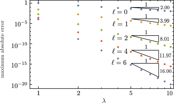
Refer to caption
Figure 3. Absolute error of HSEM expansion in the maximum norm for an interaction function s⁡(𝒚)=|𝒚|−2s(\bm{y})=|\bm{y}|^{-2} and an interpolating function gg as in (6.1) as a function of the scaling parameter λ\lambda for different expansion orders ℓ\ell.

We now approximate the two-dimensional sum of f𝒙f_{\bm{x}} over ℤ2∖{𝒙}\mathds{Z}^{2}\setminus\{\bm{x}\} by the respective Hadamard integral plus the HSEM operator of order ℓ\ell,

∑′𝒚∈ℤ2′​f𝒙​(𝒚)≈=​𝒟Λ,ν(ℓ)​g​(𝒙)+=∫ℝdg⁡(𝒚)|𝒙−𝒚|ν​𝑑𝒚.\sideset{}{{}^{\prime}}{\sum}_{\bm{y}\in\mathds{Z}^{2}}f_{\bm{x}}(\bm{y})\approx\mathrlap{\resizebox{75366}{45875}{\raisebox{2.20001pt}{{=}}}}{\mathcal{D}}_{\Lambda,\nu}^{(\ell)}g(\bm{x})+\mathchoice{{\vbox{\hbox{$\textstyle=$}}\kern-7.3611pt}}{{\vbox{\hbox{$\scriptstyle=$}}\kern-5.1528pt}}{{\vbox{\hbox{$\scriptscriptstyle=$}}\kern-4.29692pt}}{{\vbox{\hbox{$\scriptscriptstyle=$}}\kern-4.14937pt}}\!\int\limits_{\mathds{R}^{d}}\frac{g(\bm{y})}{|\bm{x}-\bm{y}|^{\nu}}\,\mathrm{d}\bm{y}.

and analyse the error for different widths λ\lambda of the interpolating function. Here, the implementation of the HSEM operator in two dimensions is discussed in Appendix A.1. For details on the computation of the Hadamard integral, see Appendix A.2.

In this formulation an additional feature of the HSEM becomes apparent. Whereas the approximate computation of the sum on the left hand side requires summation over a large number of particles NN with a computational time that increases linearly with the number of terms, the computation of the right hand side is practically indepent of NN or at most scales sublinearly with NN. The first term is a local differential operator whose coefficients depend on the lattice and can be reduced to evaluations of derivatives of the Epstein zeta function. For a large class of interpolating functions, the Hadamard integral over the whole space may be computed analytically. If this is not possible then we can exploit the convolution structure of the integral and the fact that in the case of a band-limited interpolating function, quadrature rules converge exponentially in the number of quadrature nodes as these functions are entire and band-limited.

As the scaling coefficient of the interaction, we choose the inverse square interaction22 2 We include a numerical offset of 10−310^{-3} in order to facilitate the implementation. with ν=2=d\nu=2=d, which appears in many different quantum mechanical models (see Ref. [19] and references therein), and which forms the most numerically challenging model, as both short and long-range contributions to the sum in general remain relevant and neither can be discarded. The absolute error in the maximum norm over ℤ2\mathds{Z}^{2} is displayed in Fig. 3 for different orders ℓ\ell of the HSEM operator as a function of the width λ\lambda of the interpolating function gg. The same error scaling is found for the Coulomb interaction with ν=1\nu=1 and the dipole interaction with ν=3\nu=3. The corresponding plots are provided online in our github repository. The convergence graphs for other ν∈ℂ\nu\in\mathds{C} can be efficiently generated by adapting the respective parameter for ν\nu in the Mathematica code.

We find that, to good approximation, the error scales as

Eℓ​(λ)∼λ−2​(ℓ+1),E_{\ell}(\lambda)\sim\lambda^{-2(\ell+1)},

where the exact scaling coefficients obtained from a linear fit are given in Fig. 3. This scaling law is identical to the one that we predict for the EM expansion applied to a band-limited function of sufficiently small bandwidth. Hence, the singularity of f𝒙f_{\bm{x}} has been well absorbed in the coefficients of the HSEM operator, restoring the convergence properties of the expansion. Thus, as λ→∞\lambda\to\infty, the easily computable zero order HSEM contribution already yields a good approximation to the sum. On the other hand, approximations that simply replace the sum by an integral yield an error that is independent of λ\lambda, and are therefore unreliable. For increasing HSEM orders ℓ\ell, the EM scaling law for band-limited functions is well obeyed. Already for ℓ=6\ell=6 and λ=10\lambda=10, an absolute error of less than 10−2010^{-20} is reached. The good convergence properties can be explained by the fact that the Fourier transform of Δℓ+1​g\Delta^{\ell+1}g has its mass concentrated inside the unit ball, with only a small high frequency correction. Thus, the function essentially behaves as if it belonged to EσE_{\sigma} with σ<aΛ∗=1\sigma<a_{\Lambda^{*}}=1 and only for very large orders ℓ\ell, the convergence breaks down. The HSEM works well, as long as the interpolating function gg, which in many cases is an interpolation of discrete particle positions, does not exhibit oscillations in space whose inverse wavelengths exceed aΛ∗a_{\Lambda^{*}}. These oscillations would exhibit wavelengths that are smaller than the unit lattice cell and would therefore be unphysical. Thus, the HSEM converges for physically meaningful interpolation functions gg, allowing us to approximate singular sums in arbitrary dimensions independently of the particle number.

7. Conclusions and outlook

In this work, we have extended the Euler–Maclaurin (EM) summation formula to lattices in higher dimensions. We have then subsequently used the EM expansion as a tool in the proof of the multidimensional singular Euler–Maclaurin (SEM) expansion that allows for the inclusion of singular factors in the summand function and thus makes the formula applicable to interaction functions that appear in physical applications. This is for instance the case in a solid state system with Coulomb or dipolar particle interactions. In order to avoid the evaluation of oscillatory surface integrals and make the expansion easy to use in practice, we have gone one step further and have introduced the hypersingular Euler–Maclaurin (HSEM) expansion, where the differential operator is local with coefficients that can be evaluated using standard techniques from number theory. We have designed the SEM and HSEM expansion as mathematical tools that can immediately be applied to open questions in physics. It is our hope that the SEM and HSEM expansion will find use in the precise evaluation of long-range forces and energies in crystal and spin lattices, in the evaluation of high-dimensional partition functions in statistical physics, and in the quantification of discreteness effects in fundamental physics.

We expect that the summation formulas developed in this paper can be further generalised to quasi-crystals, like the Penrose lattice, and to statistical distributions of particles. We also consider it to be worthwhile to investigate solution techniques for the integro-differential equations that follow from the HSEM expansion, for instance in the context of spin waves.

Acknowledgements

We would like to thank our colleagues Daniel Seibel, Christian Michel, and Peter Schuhmacher for proof-reading the manuscript and for helpful suggestions. We thank Prof. Sergej Rjasanow for insightful discussions and for his support.

Appendix A HSEM expansion in two dimensions

A.1. HSEM operator coefficients

For a square lattice in d=2d=2 dimensions, a simple approach for generating the HSEM operator coefficients is available that avoids derivatives of Epstein zeta functions and uses efficient summation formulas that have been found in the analysis of the Riemann hypothesis in higher dimensions [24]. For a two-dimensional square lattice, it has been shown that [34, Eq. (9)]

∑′𝒛∈ℤ2′​1|𝒛|ν=4​ζ​(ν/2)​βD​(ν/2),\sideset{}{{}^{\prime}}{\sum}_{\bm{z}\in\mathds{Z}^{2}}\frac{1}{|\bm{z}|^{\nu}}=4\zeta(\nu/2)\beta_{D}(\nu/2),

where βD\beta_{D} is the Dirichlet beta function and where the Dirichlet series can be extended to ν∈ℂ∖{2}\nu\in\mathds{C}\setminus\{2\}. Furthermore, the meromorphic continuation of the lattice sum

Cn​(ν)=∑′𝒛∈ℤ2′​z12​n|𝒛|ν+2​n,ν∈ℂ∖{2},C_{n}(\nu)=\sideset{}{{}^{\prime}}{\sum}_{\bm{z}\in\mathds{Z}^{2}}\frac{z_{1}^{2n}}{|\bm{z}|^{\nu+2n}},\quad\nu\in\mathds{C}\setminus\{2\},

has been shown to be computable for n∈ℕ+n\in\mathds{N}_{+} via the formula [24, Eq. (2.3)]

Cn​(ν)\displaystyle C_{n}(\nu) =2​π​Γ​(ν/2+n−1/2)​ζ​(ν−1)Γ⁡(ν/2+n)\displaystyle=\frac{2\sqrt{\pi}\,\Gamma(\nu/2+n-1/2)\zeta(\nu-1)}{\Gamma(\nu/2+n)}
+8​πν/2Γ⁡(ν/2+n)∑z1=1∞∑z2=1∞(z2z1)(ν−1)/2(z1z2π)nK(ν−1)/2+n(2πz1z2),\displaystyle+\frac{8\pi^{\nu/2}}{\Gamma(\nu/2+n)}\sum_{z_{1}=1}^{\infty}\sum_{z_{2}=1}^{\infty}\bigg(\frac{z_{2}}{z_{1}}\bigg)^{(\nu-1)/2}(z_{1}z_{2}\pi)^{n}K_{(\nu-1)/2+n}(2\pi z_{1}z_{2}),

with Kν​(x)K_{\nu}(x) the modified Bessel function of the second kind. As the double sum converges exponentially fast in both variables, the lattice sum can be efficiently approximated. We now show that, using the above two lattice sums, we can generate the whole HSEM operator in d=2d=2 dimensions by using an expansion in solid harmonics.

First note that for k>0k>0, only even kk lead to a nonzero contribution due to symmetry of the interaction. Setting k=2​nk=2n, with n∈ℕn\in\mathds{N}, we then find

limβ→0∑=∫𝐳∈ℝ2,ℤ2⁡χ^β​(𝐳)​⟨𝐳,∇⟩2​n|𝐳|ν\displaystyle\lim_{\beta\to 0}\SumDDInt_{\bm{z}\in\mathds{R}^{2},\mathds{Z}^{2}}\hat{\chi}_{\beta}(\bm{z})\frac{\langle\bm{z},\nabla\rangle^{2n}}{|\bm{z}|^{\nu}}
=∑m=0na2​m(2​n)​limβ→0∑=∫𝐳∈ℝ2,ℤ2⁡χ^β​(𝐳)​|𝐳|2​(n−m)​A2​m​(𝐳)|𝐳|ν​A2​(n−m)​(∇)​Δn−m,\displaystyle=\sum_{m=0}^{n}a^{(2n)}_{2m}\lim_{\beta\to 0}\SumDDInt_{\bm{z}\in\mathds{R}^{2},\mathds{Z}^{2}}\hat{\chi}_{\beta}(\bm{z})\frac{|\bm{z}|^{2(n-m)}A_{2m}(\bm{z})}{|\bm{z}|^{\nu}}A_{2(n-m)}(\nabla)\Delta^{n-m},

with the solid harmonic Ak:ℝ2→ℝA_{k}:\mathds{R}^{2}\to\mathds{R},

Ak​(𝒚)=Re⁡((y1+i​y2)k),A_{k}(\bm{y})=\mathrm{Re}\Big((y_{1}+iy_{2})^{k}\Big),

and

a0(k)=12​π∫02​πcos(ϕ)kdϕ,an(k)=1π∫02​πcos(nϕ)cos(ϕ)kdϕ.a_{0}^{(k)}=\frac{1}{2\pi}\int\limits_{0}^{2\pi}\cos(\phi)^{k}\,\text{d}\phi,\qquad a_{n}^{(k)}=\frac{1}{\pi}\int\limits_{0}^{2\pi}\cos(n\phi)\cos(\phi)^{k}\,\text{d}\phi.

Finally,

(A.1) ∑′𝒛∈ℤ2′​A2​m​(𝒛)|𝒛|ν+2​m=Z0​(I2,ν)+∑k=1m1(2​k)!​T2​m(2​k)​(0)​Ck​(ν),\,\sideset{}{{}^{\prime}}{\sum}_{\bm{z}\in\mathds{Z}^{2}}\frac{A_{2m}(\bm{z})}{|\bm{z}|^{\nu+2m}}=Z_{0}(I_{2},\nu)+\sum_{k=1}^{m}\frac{1}{(2k)!}T_{2m}^{(2k)}(0)\,C_{k}(\nu),

where I2∈ℝ2×2I_{2}\in\mathds{R}^{2\times 2} denotes the identity matrix and TmT_{m} is the Chebyshev polynomial of the first kind of order mm. To prove this, we use that

A2​m​(𝒛)=|𝒛|2​m​cos⁡(2​m​ϕ)A_{2m}(\bm{z})=|\bm{z}|^{2m}\cos(2m\phi)

for the polar angle ϕ\phi, 𝒛=|𝒛|(cos⁡ϕ,sin⁡ϕ)\bm{z}=|\bm{z}|(\cos\phi,\sin\phi). Now, cos⁡(2​m​ϕ)\cos(2m\phi) can be expanded into powers of cos⁡ϕ\cos\phi by means of the Chebyshev polynomial T2​mT_{2m},

cos(2mϕ)=T2​m(cosϕ)=∑k=02​mT2​m(k)cos(ϕ)k.\cos(2m\phi)=T_{2m}(\cos\phi)=\sum_{k=0}^{2m}T_{2m}^{(k)}\cos(\phi)^{k}.

Inserting this into the right hand side of (A.1), observing that odd orders vanish due to the symmetry of the lattice and furthermore

|𝒛|2​k​(cos⁡ϕ)2​k=z12​k,|\bm{z}|^{2k}(\cos\phi)^{2k}=z_{1}^{2k},

yields the desired equality.

A.2. Evaluation of the Hadamard integral

We briefly discuss how the Hadamard integral is evaluated. For the special choice of gg in (6.1) and d=2d=2, we can determine the Hadamard integral analytically. As g∈S⁡(ℝd)g\in S(\mathds{R}^{d}), we have that

=∫ℝdg⁡(𝒚)|𝒙−𝒚|νd𝒚=ℱ((ℱ|⋅|−ν)(ℱg))(𝒙),\mathchoice{{\vbox{\hbox{$\textstyle=$}}\kern-7.3611pt}}{{\vbox{\hbox{$\scriptstyle=$}}\kern-5.1528pt}}{{\vbox{\hbox{$\scriptscriptstyle=$}}\kern-4.29692pt}}{{\vbox{\hbox{$\scriptscriptstyle=$}}\kern-4.14937pt}}\!\int\limits_{\mathds{R}^{d}}\frac{g(\bm{y})}{|\bm{x}-\bm{y}|^{\nu}}\,\mathrm{d}\bm{y}=\mathcal{F}\Big((\mathcal{F}|\bm{\cdot}|^{-\nu})(\mathcal{F}g)\Big)(\bm{x}),

where we have applied the convolution theorem for distributions. We then find

=∫ℝdg⁡(𝒚)|𝒙−𝒚|ν​𝑑𝒚=π​Γ​(1−ν/2)λν−2​M​(ν/2,1,−|𝒙/λ|2),\mathchoice{{\vbox{\hbox{$\textstyle=$}}\kern-7.3611pt}}{{\vbox{\hbox{$\scriptstyle=$}}\kern-5.1528pt}}{{\vbox{\hbox{$\scriptscriptstyle=$}}\kern-4.29692pt}}{{\vbox{\hbox{$\scriptscriptstyle=$}}\kern-4.14937pt}}\!\int\limits_{\mathds{R}^{d}}\frac{g(\bm{y})}{|\bm{x}-\bm{y}|^{\nu}}\,\mathrm{d}\bm{y}=\frac{\pi\Gamma(1-\nu/2)}{\lambda^{\nu-2}}M\big(\nu/2,1,-|\bm{x}/\lambda|^{2}\big),

with MM the Kummer confluent hypergeometric function [27, Eq. (13.2.2)].

References

  • [1] T. M. Apostol, Introduction to Analytic Number Theory, Undergraduate Texts in Mathematics, Springer New York, 1998.
  • [2] by same author, An Elementary View of Euler’s Summation Formula, The American Mathematical Monthly 106 (1999), no. 5, 409–418.
  • [3] N. Aronszajn, T.M. Creese, and L.J. Lipkin, Polyharmonic Functions, Oxford mathematical monographs, Clarendon Press, 1983.
  • [4] J. Borwein, M. Glasser, R. McPhedran, J. Wan, and I. Zucker, Lattice Sums Then and Now, Encyclopedia of Mathematics and its Applications, Cambridge University Press, 2013.
  • [5] Andreas A. Buchheit and Torsten Keßler, Singular Euler-Maclaurin expansion, (2020).
  • [6] A. Campa, T. Dauxois, D. Fanelli, and S. Ruffo, Physics of long-range interacting systems, OUP Oxford, 2014.
  • [7] M. Dupuis, J.P. Ryan, S. Speziale, et al., Discrete gravity models and loop quantum gravity: a short review, SIGMA. Symmetry, Integrability and Geometry: Methods and Applications 8 (2012), 052.
  • [8] E. Elizalde, Zeta functions: formulas and applications, Journal of Computational and Applied Mathematics 118 (2000), no. 1-2, 125–142.
  • [9] O. Emersleben, Zetafunktionen und elektrostatische Gitterpotentiale. I, Phys. Z 24 (1923), 73–80.
  • [10] by same author, Zetafunktionen und elektrostatische Gitterpotentiale. II, Phys. Z 24 (1923), 97–104.
  • [11] P. Epstein, Zur Theorie allgemeiner Zetafunktionen. I, Math. Ann. 56 (1903), 615–644.
  • [12] by same author, Zur Theorie allgemeiner Zetafunktionen. II, Math. Ann. 63 (1906), 205–216.
  • [13] W. Freeden, Metaharmonic lattice point theory, CRC Press, 2011.
  • [14] R.H. French et al., Long range interactions in nanoscale science, Reviews of Modern Physics 82 (2010), no. 2, 1887.
  • [15] I. M. Gel’fand and G. E. Shilov, Generalized functions, Academic Press, 1964.
  • [16] M. Gibertini, M. Koperski, A.F. Morpurgo, and K.S. Novoselov, Magnetic 2D materials and heterostructures, Nature nanotechnology 14 (2019), no. 5, 408–419.
  • [17] D. Gilbarg and N. S. Trudinger, Elliptic Partial Differential Equations of Second Order, Springer-Verlag, 1998.
  • [18] H. Groemer, Geometric Applications of Fourier Series and Spherical Harmonics, Cambridge University Press, 1996.
  • [19] K.S. Gupta, Quantum inverse square interaction, Modern Physics Letters A 18 (2003), 2355–2362.
  • [20] L. Hörmander, The Analysis of Linear Partial Differential Operators I: Distribution Theory and Fourier Analysis, Classics in Mathematics, Springer, 2003.
  • [21] by same author, The Analysis of Linear Partial Differential Operators III: Pseudo–Differential Operators, Classics in Mathematics, Springer, 2007.
  • [22] Y. Karshon, S. Sternberg, and J. Weitsman, Exact Euler–Maclaurin formulas for simple lattice polytopes, Advances in Applied Mathematics 39 (2007), no. 1, 1–50.
  • [23] W. McLean, Strongly elliptic systems and boundary integral equations, Cambridge University Press, 2000.
  • [24] R.C. McPhedran, I.J. Zucker, L.C. Botten, and N.P. Nicorovici, On the Riemann property of angular lattice sums and the one-dimensional limit of two-dimensional lattice sums, Proceedings of the Royal Society A: Mathematical, Physical and Engineering Sciences 464 (2008), no. 2100, 3327–3352.
  • [25] G. Monegato and J. N. Lyness, The Euler-Maclaurin expansion and finite-part integrals, Numerische Mathematik 81 (1998), no. 2, 273–291.
  • [26] C. Müller, Eine Verallgemeinerung der Eulerschen Summenformel und ihre Anwendung auf Fragen der analytischen Zahlentheorie, Abhandlungen aus dem Mathematischen Seminar der Universität Hamburg, vol. 19, Springer, 1954, pp. 41–62.
  • [27] F.W. Olver, D.W. Lozier, R.F. Boisvert, and C.W. Clark, Nist handbook of mathematical functions, Cambridge University Press, 2010.
  • [28] A. Perez and D. Sudarsky, Dark energy from quantum gravity discreteness, Physical Review Letters 122 (2019), no. 22, 221302.
  • [29] C. Rovelli and S. Speziale, Reconcile Planck-scale discreteness and the Lorentz-Fitzgerald contraction, Physical Review D 67 (2003), no. 6, 064019.
  • [30] J. Smit, Introduction to quantum fields on a lattice, Cambridge University Press, 2002.
  • [31] E. M. Stein and G. Weiss, Introduction to Fourier Analysis on Euclidean Spaces, Princeton University Press, 1972.
  • [32] F. Trèves, Topological vector spaces, distributions and kernels, Academic Press, 1967, Reprinted by Dover, 2006.
  • [33] by same author, Basic linear partial differential equations, Academic Press, 1975, Reprinted by Dover, 2006.
  • [34] I.J. Zucker, The Exact Evaluation of Some New Lattice Sums, Symmetry 9 (2017), no. 12, 314.